Towards Using Unlabeled Data in a Sparse-coding Framework for Human Activity Recognition

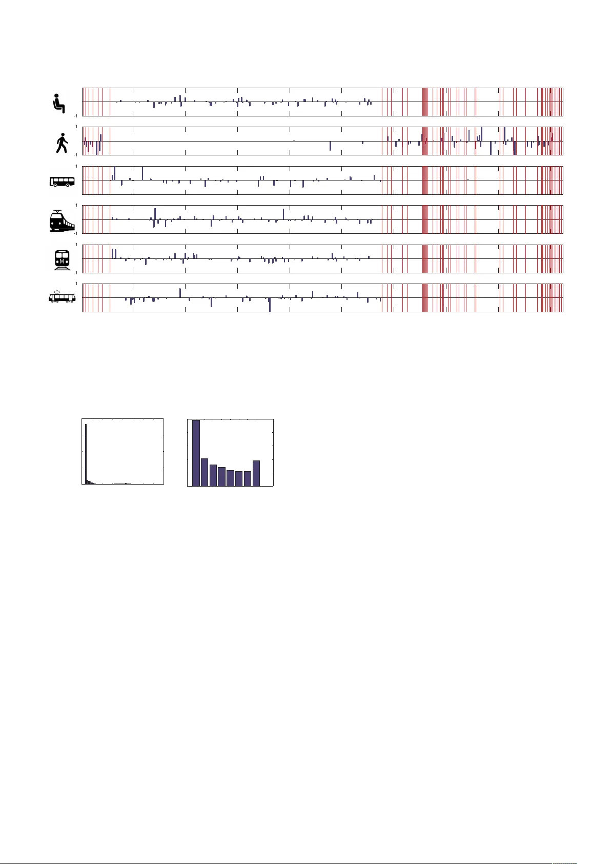
!!!!!!!!!!!!!! ! ! ! ! Towards Using Unl abeled Data in a Spar se - coding Framework for Human Activit y Recognition Sourav Bhattacharya a , Petteri Nurmi a , Nils Hammerla b , and Thomas Plötz b a Helsinki Institute for Information Technology HIIT, Department of Computer Science, University of Helsinki, Finland b Culture Lab, School of Computing Science, Newcastle University, UK ! “NOTICE: this is the author’s version of a work that was accepted for publication in Pervasive and Mobile Computing . Changes resulting from the publishing process, such as peer review, editing, corrections, structural formatting, and other quality control m echanisms may not be reflected in this document. Changes may have been made to this work since it was submitted for publication. DOI: 10.1016/j.pmcj.2014.05.006 ” T o wards Using Unlabeled Data in a Sparse-coding Frame work for Human Acti vity Recognition Sourav Bhattacharya a , Petteri Nurmi a , Nils Hammerla b , Thomas Pl ¨ otz b a Helsinki Institute for Information T ec hnology HIIT Department of Computer Science, University of Helsinki, F inland b Cultur e Lab, School of Computing Science, Newcastle University , UK Abstract W e propose a sparse-coding framew ork for activity recognition in ubiquitous and mobile computing that alleviates two fundamental problems of current supervised learning approaches. (i) It automatically deri ves a compact, sparse and meaningful feature representation of sensor data that does not rely on prior expert knowledge and generalizes well across domain boundaries. (ii) It exploits unlabeled sample data for bootstrapping ef fective activity recognizers, i.e., substantially reduces the amount of ground truth annotation required for model estimation. Such unlabeled data is easy to obtain, e.g., through contemporary smartphones carried by users as they go about their e veryday acti vities. Based on the self-taught learning paradigm we automatically deriv e an over -complete set of basis vectors from un- labeled data that captures inherent patterns present within activity data. Through projecting raw sensor data onto the feature space defined by such ov er-complete sets of basis vectors effecti ve feature extraction is pursued. Gi ven these learned feature representations, classification backends are then trained using small amounts of labeled training data. W e study the new approach in detail using two datasets which dif fer in terms of the recognition tasks and sensor modalities. Primarily we focus on a transportation mode analysis task, a popular task in mobile-phone based sens- ing. The sparse-coding framew ork demonstrates better performance than the state-of-the-art in supervised learning approaches. More importantly , we show the practical potential of the ne w approach by successfully ev aluating its gen- eralization capabilities across both domain and sensor modalities by considering the popular Opportunity dataset. Our feature learning approach outperforms state-of-the-art approaches to analyzing acti vities of daily li ving. K eywor ds: Acti vity Recognition, Sparse-coding, Machine Learning, Unsupervised Learning. 1. Intr oduction Acti vity recognition represents a major research area within mobile and pervasi ve/ubiquitous computing [1, 3]. Prominent examples of domains where activity recogni- tion has been in vestigated include smart homes [4, 5, 6], situated support [7], automatic monitoring of mental and physical wellbeing [8, 9, 10], and general health care [11, 12]. Modern smartphones with their advanced sensing capabilities provide a particularly attracti ve platform for acti vity recognition as they are carried around by many people while going about their e veryday acti vities. The vast majority of activity recognition research re- lies on supervised learning techniques where handcrafted features, e.g., heuristically chosen statistical measures, are extracted from raw sensor recordings, which are then combined with acti vity labels for ef fectiv e classifier train- ing. While this approach is in line with the standard procedures in many application domains of general pat- tern recognition and machine learning techniques [13], it is often too costly or simply not applicable for ubiqui- tous/perv asi ve computing applications. The reasons for this are twofold. Firstly , the performance of supervised learning approaches is highly sensitive to the type of fea- ture extraction, where often the optimal set of features v aries across different acti vities [14, 15, 16]. Secondly , and more crucially , obtaining reliable ground truth anno- tation for bootstrapping and training acti vity recognizers poses a challenge for system dev elopers who target real- world deployments. People typically carry their mobile de vice while going about their e veryday acti vities, thereby not paying much attention to the phone itself in terms of location of the de vice (in the pocket, in the backpack, etc.) and only sporadically interacting with it (for making a call or explicitly using the de vice’ s services for , e.g., informa- Pr eprint submitted to P ervasive and Mobile Computing J uly 24, 2014 tion retrie v al). Consequently , activ e support from users to provide labels for data collected in real-life scenarios can- not be considered feasible for many settings as prompting mobile phone users to annotate their activities while they are pursuing them has its limitations. Apart from these limitations, priv acy and ethical considerations typically render direct observation and annotation impracticable in realistic scenarios. Possible alternativ es to such direct observ ation and an- notation include: (i) self-reporting of activities by the users, e.g., using a diary [17]; (ii) the use of experience sampling, i.e., prompting the user and asking for the cur- rent or pre vious activity label [4, 18]; and (iii) a combina- tion of these methods. While such techniques somewhat alle viate the aforementioned problem by providing anno- tation for at least smaller subsets of unlabeled data, they still remain prone to errors and typically cannot replace expert ground truth annotation. Whereas obtaining reliable ground truth annotation is hard to achieve, the collection of, ev en large amounts of, unlabeled sample data is typically straightforward. Peo- ple’ s smartphones can simply record acti vity data in an opportunistic way , without requiring the user to follow a certain protocol or scripted acti vity patterns. This is espe- cially attracti ve since it allows for capturing sensor data while users perform their natural acti vities without neces- sarily being conscious about the actual data collection. In this paper we introduce a nov el framew ork for acti v- ity recognition. Our approach mitigates the requirement of large amounts of ground truth annotation by explic- itly exploiting unlabeled sensor data for bootstrapping our recognition framew ork. Based on the self-taught learn- ing paradigm [19], we develop a sparse-coding frame- work for unsupervised estimation of sensor data repre- sentations with the help of a codebook of basis vectors (see Section 3.2). As these representations are learned in an unsupervised manner , our approach also ov ercomes the need to perform feature-engineering. While the origi- nal frame work of self-taught learning has been dev eloped mainly for the analysis of non-sequential data, i.e., images and stationary audio signals [20], we extend the approach to wards time-series data such as continuous sensor data streams. W e also de velop a basis selection method that builds on information theory to generate a codebook of basis v ectors that covers characteristic mov ement patterns in human physical acti vities. Using activations of these basis vectors (see Section 3.3) we then compute features of the raw sensor data streams, which are the basis for subsequent classifier training. The latter requires only rel- ati vely small amounts of labeled data, which alle viates the ground truth annotation challenge of mobile computing applications. W e demonstrate the benefits of our approach using data from two di verse acti vity recognition tasks, namely trans- portation mode analysis and classification of activities of daily li ving (the Opportunity challenge [21]). Our e x- periments demonstrate that the proposed approach pro- vides better results than the state-of-the-art, namely PCA- based feature learning, semi-supervised En-Co-T raining, and feature-engineering based (supervised) algorithms, while requiring smaller amounts of training data and not relying on prior domain kno wledge for feature crafting. Apart from successful generalization across recognition tasks, we also demonstrate easy applicability of our pro- posed framework beyond modality boundaries covering not only accelerometer data but also other commonly av ailable sensors on the mobile platform, such as the gy- roscopes, or magnetometers. 2. Learning From Unlabeled Data The focus of our work is on developing an effecti ve frame work that exploits unlabeled data to deri ve robust acti vity recognizers for mobile applications. The key idea is to use vast amounts of easy to record unlabeled sam- ple data for unsupervised featur e learning . These features shall cov er general characteristics of human movements, which guarantees both robustness and generalizability . Only very little related work exists that focus on incor- porating unlabeled data for training mobile activity rec- ognizers. A notable exception is the work by Amft who explored self-taught learning in a very preliminary study for activity spotting using on-body motion sensors [22]. Ho we ver , that work does not take into account the proper - ties of the learned codebook which play an important role in the recognition task. The idea of incorporating unlabeled data and related feature learning techniques into recognizer training is a well researched area in the general machine learning and pattern recognition community . In the following, we will summarize rele vant related work from these fields and link them to the mobile and ubiquitous computing domain. 2.1. Non-supervised Learning P aradigms A number of general learning paradigms hav e been de- veloped that focus on deri ving statistical models and rec- ognizers by incorporating unlabeled data. Although dif- fering in their particular approaches, all related techniques share the objectiv e of alleviating the dependence on a 3 large amount of annotated training data for parameter es- timation. Learning from a combination of labeled and unlabeled datasets is commonly known as semi-supervised learn- ing [23]. The most common approach to semi-supervised learning is generative models , where the unkno wn data distribution p ( x ) is modeled as a mixture of class condi- tional distributions p ( x | y ) , where y is the (unobserved) class variable. The mixture components are estimated from a large amount of unlabeled and small amount of labeled data by applying the Expectation Maximization (EM) algorithm. The predictiv e estimate of p ( y | x ) is then computed using Bayes’ formula. Other approaches to semi-supervised learning include self-training , co- training , transductive SVM (TSVM), graphical models and multiview learning . Semi-supervised learning techniques hav e also been ap- plied to activity recognition, e.g., for recognizing loco- motion related activities [24], and in smart homes [25]. In order to be effecti ve, semi-supervised learning approaches need to satisfy certain, rather strict assumptions [23, 26]. Probably the strongest constraint imposed by these tech- niques is that they assume that the unlabeled and la- beled datasets are drawn from the same distribution, i.e., D u = D l . In other words, the unlabeled dataset has to be collected with strict focus on the set of acti vities the recognizer shall cov er . This limits generalization capabil- ity and renders the learning error-prone for real-world set- tings where the user might perform extraneous activities, or no acti vity at all [27]. Our approach provides improved generalization capability by relaxing the equality condi- tion for the distributions of unlabeled and labeled datasets, i.e., D u 6 = D l . An alternative approach to dealing with unlabeled data is active learning . T echniques for acti ve learning aim to make the most economic use of annotations by identifying those unlabeled samples that are most uncertain and thus their annotation would provide most information for the training process. Such samples are automatically iden- tified using information theoretic criteria and then man- ual annotation is requested. Acti ve learning approaches hav e become very popular in a number of application domains including activity recognition using body-worn sensors [30, 25]. Activ e learning operates on pre-defined sets of features, which stands in contrast to our approach that automatically learns feature representations. In do- ing so, activ e learning becomes sensitiv e to the particular features that hav e been e xtracted, hence limiting its gen- eralizability . Explicitly focusing on generalizability of recognition frame works, transfer learning techniques hav e been de- veloped to bridge, e.g., application domains with differ - ing classes or sensing modalities [31]. In this approach, kno wledge acquired in a specific domain can be trans- ferred to another , if a systematic transformation is either provided or learned automatically . Transfer learning has been applied to ubiquitous computing problems, for ex- ample, for adapting models learned with data from one smart home to work within another smart home [32, 33], or to adapt acti vity classifiers learned with data from one user to work with other users [34]. In these approaches the need for annotated training data is not directly reduced but shifted to other domains or modalities, which can be beneficial if such data are easier to obtain. As an alternative approach to alle viating the demands of ground truth annotation so-called multi-instance learn- ing techniques have been dev eloped. These techniques assign labels to sets of instances instead of indi vidual data points [35]. Multi-instance learning has also been applied for acti vity recognition tasks in ubiquitous computing set- tings [18, 36]. T o apply multi-instance learning, labels of the indi vidual instances were considered as hidden v ari- ables and a support vector machine was trained to min- imize the expected loss of the classification of instances using the labels of the instance sets. Multi-instance learn- ing also operates on a predefined set of features and there- fore has limited generalizability . 2.2. F eatur e Learning Exploiting unlabeled data can also be applied at the fea- ture lev el to deri ve a compact and meaningful representa- tion of raw input data. In fact, feature learning, i.e., un- supervised estimation of suitable data representations, has been acti vely researched in the machine learning commu- nity [37]. The goal of feature learning is to identify and model interesting regularities in the sensor data without being driven by class information. The majority of meth- ods rely on a process similar to generativ e models b ut em- ploy efficient, approximativ e learning algorithms instead of EM [38]. Data representations for activity recognition in the ubiquitous or mobile computing domain typically corre- spond to some sort of “engineered” feature sets, e.g., sta- tistical values calculated ov er analysis windows that are extracted using a sliding window procedure [14]. Such predefined features often do not generalize across domain boundaries, which requires system dev elopers to optimize their data representation virtually from scratch for e very ne w application domain. 4 Only recently , concepts of feature learning have been successfully applied for activity recognition tasks. For example, M ¨ antyj ¨ arvi et al. [39] compared the use of Prin- cipal Component Analysis (PCA) and Independent Com- ponent Analysis (ICA) for e xtracting features from sensor data. In their approach, either PCA or ICA w as applied on raw sensor v alues. A sliding windo w was then applied on the transformed data and a W avelet-based feature extrac- tion method was used in combination with a multilayer perceptron. Similarly , Pl ¨ otz et al. employed principal component analysis to deri ve features from tri-axial accelerometer data using a sliding window approach [40]. Howe ver , in- stead of applying the PCA on the raw sensor values, they used the empirical cumulativ e distrib ution of a data frame to represent the signals before applying PCA [42]. More- ov er , they in vestigated the use of Restricted Boltzmann Machines [38], to train an autoencoder network for fea- ture learning. Minnen et al. [43] considered activities as sparse motifs in multidimensional time series and proposed an unsuper - vised algorithm for automatically extracting such motifs from data. A related approach was proposed by Frank et al. [44] who used time-delay embeddings to e xtract fea- tures from windo wed data and fed these features to a sub- sequent classifier . Contrary to the popular Fourier and W avelet representa- tions, which suf fer from non-adaptability to the particular dataset [45], we employ a data-adapti ve approach of rep- resenting accelerometer measurements. The data-adaptiv e representation is tailored to the statistics of the data and is directly learned from the recorded measurements. Ex- amples of data-adaptiv e methods include PCA, ICA and Matrix Factorization. Our approach dif fers from common data-adapti ve methods by employing an over -complete and sparse feature representation technique. Here, ov er - completeness indicates that the dimension of the feature space is much higher than the original input data dimen- sion, and sparsity indicates that the majority of the ele- ments in a feature vector is zero. 3. A Sparse-Coding Framework for Activity Recognition W e propose a sparse-coding frame work for activity recognition that uses a codebook of basis vectors that cap- ture characteristic and latent patterns in the sensor data. As the codebook learning is unsupervised and operates on unlabeled data, our approach effecti vely reduces the need for annotated ground truth data and ov ercomes the need to use predefined feature representations, rendering our approach well suited for continuous activity recognition tasks under naturalistic settings. 3.1. Method Overview Figure 1 giv es an ov ervie w of our approach to learn- ing acti vity recognizers. W e first collect unlabeled data, which in our experiments consists mainly of tri-axial ac- celerometer measurements (upper part of Figure 1(a)). W e then solve an optimization problem (see Section 3.2) to learn a set of basis vectors — the codebook — that cap- ture characteristic patterns of human movements as the y can be observed from the raw sensor data (lower part of Figure 1(a)). Once the codebook has been learned, we use a small set of labeled data to train an acti vity classifier (Figure 1(b)). The features that are used for training the classifier cor - respond to so-called activations , which are vectors that enable transferring sensor readings to the feature space spanned by the basis vectors in the codebook. After model training, the activity label for new sensor readings can be determined by transferring the corresponding mea- surements into the same feature space and applying the learned classifier . 3.2. Codebook Learning fr om Unlabeled Data W e consider sequential, multidimensional sensor data, which in our experiments correspond to measurements from a tri-axial accelerometer or a gyroscope. W e ap- ply a sliding windo w procedure on the measurements to extract overlapping, fixed length frames. Specifically , we consider measurements of the form x i ∈ R n , where x i is a v ector containing all measurements within the i th frame and n is the length of the frame, i.e., the unlabeled mea- surements are represented as the set X = { x 1 , x 2 , . . . , x K } , x i ∈ R n . (1) In the first step of our approach, we use the unlabeled data X to learn a codebook B that captures latent and characteristic patterns in the sensor measurements. The codebook consists of S basis vectors { β j } S j =1 , where each basis vector β j ∈ R n represents a particular pattern in the data. Once the codebook has been learned, any frame of sensor measurements can be represented as a linear super- position of the basis vectors, i.e., x i ≈ S X j =1 a i j β j , (2) 5 Unlabeled data 10 20 30 40 50 60 70 80 90 100 -0.5 0 0.5 B 1 10 20 30 40 50 60 70 80 90 100 -0.5 0 0.5 B 2 10 20 30 40 50 60 70 80 90 100 -0.5 0 0.5 B 3 10 20 30 40 50 60 70 80 90 100 -0.5 0 0.5 B 4 10 20 30 40 50 60 70 80 90 100 -0.5 0 0.5 B 5 10 20 30 40 50 60 70 80 90 100 -0.5 0 0.5 B 6 10 20 30 40 50 60 70 80 90 100 -0.5 0 0.5 B 7 10 20 30 40 50 60 70 80 90 100 -0.5 0 0.5 B 8 10 20 30 40 50 60 70 80 90 100 -0.5 0 0.5 B 9 10 20 30 40 50 60 70 80 90 100 -0.5 0 0.5 B 10 10 20 30 40 50 60 70 80 90 100 -0.5 0 0.5 B 11 10 20 30 40 50 60 70 80 90 100 -0.5 0 0.5 B 12 10 20 30 40 50 60 70 80 90 100 -0.5 0 0.5 B 13 10 20 30 40 50 60 70 80 90 100 -0.5 0 0.5 B 14 10 20 30 40 50 60 70 80 90 100 -0.5 0 0.5 B 15 10 20 30 40 50 60 70 80 90 100 -0.5 0 0.5 B 16 10 20 30 40 50 60 70 80 90 100 -0.5 0 0.5 B 17 10 20 30 40 50 60 70 80 90 100 -0.5 0 0.5 B 18 10 20 30 40 50 60 70 80 90 100 -0.5 0 0.5 B 19 10 20 30 40 50 60 70 80 90 100 -0.5 0 0.5 B 20 10 20 30 40 50 60 70 80 90 100 -0.5 0 0.5 B 21 10 20 30 40 50 60 70 80 90 100 -0.5 0 0.5 B 22 10 20 30 40 50 60 70 80 90 100 -0.5 0 0.5 B 23 10 20 30 40 50 60 70 80 90 100 -0.5 0 0.5 B 24 10 20 30 40 50 60 70 80 90 100 -0.5 0 0.5 B 25 10 20 30 40 50 60 70 80 90 100 -0.5 0 0.5 B 26 10 20 30 40 50 60 70 80 90 100 -0.5 0 0.5 B 27 10 20 30 40 50 60 70 80 90 100 -0.5 0 0.5 B 28 10 20 30 40 50 60 70 80 90 100 -0.5 0 0.5 B 29 10 20 30 40 50 60 70 80 90 100 -0.5 0 0.5 B 30 10 20 30 40 50 60 70 80 90 100 -0.5 0 0.5 B 31 10 20 30 40 50 60 70 80 90 100 -0.5 0 0.5 B 32 10 20 30 40 50 60 70 80 90 100 -0.5 0 0.5 B 33 10 20 30 40 50 60 70 80 90 100 -0.5 0 0.5 B 34 10 20 30 40 50 60 70 80 90 100 -0.5 0 0.5 B 35 10 20 30 40 50 60 70 80 90 100 -0.5 0 0.5 B 36 10 20 30 40 50 60 70 80 90 100 -0.5 0 0.5 B 37 10 20 30 40 50 60 70 80 90 100 -0.5 0 0.5 B 38 10 20 30 40 50 60 70 80 90 100 -0.5 0 0.5 B 39 10 20 30 40 50 60 70 80 90 100 -0.5 0 0.5 B 40 10 20 30 40 50 60 70 80 90 100 -0.5 0 0.5 B 41 10 20 30 40 50 60 70 80 90 100 -0.5 0 0.5 B 42 10 20 30 40 50 60 70 80 90 100 -0.5 0 0.5 B 43 10 20 30 40 50 60 70 80 90 100 -0.5 0 0.5 B 44 10 20 30 40 50 60 70 80 90 100 -0.5 0 0.5 B 45 10 20 30 40 50 60 70 80 90 100 -0.5 0 0.5 B 46 10 20 30 40 50 60 70 80 90 100 -0.5 0 0.5 B 47 10 20 30 40 50 60 70 80 90 100 -0.5 0 0.5 B 48 10 20 30 40 50 60 70 80 90 100 -0.5 0 0.5 B 49 10 20 30 40 50 60 70 80 90 100 -0.5 0 0.5 B 50 10 20 30 40 50 60 70 80 90 100 -0.5 0 0.5 B 51 10 20 30 40 50 60 70 80 90 100 -0.5 0 0.5 B 52 10 20 30 40 50 60 70 80 90 100 -0.5 0 0.5 B 53 10 20 30 40 50 60 70 80 90 100 -0.5 0 0.5 B 54 10 20 30 40 50 60 70 80 90 100 -0.5 0 0.5 B 55 10 20 30 40 50 60 70 80 90 100 -0.5 0 0.5 B 56 1 0 2 0 30 4 0 50 60 7 0 80 90 1 00 -0.5 0 0.5 B 57 1 0 2 0 30 4 0 50 60 7 0 80 90 1 00 -0.5 0 0.5 B 58 1 0 2 0 30 4 0 50 60 7 0 80 90 1 00 -0.5 0 0.5 B 59 1 0 2 0 30 4 0 50 60 7 0 80 90 1 00 -0.5 0 0.5 B 60 1 0 2 0 30 4 0 50 60 7 0 80 90 1 00 -0.5 0 0.5 B 61 1 0 2 0 30 4 0 50 60 7 0 80 90 1 00 -0.5 0 0.5 B 62 1 0 2 0 30 4 0 50 60 7 0 80 90 1 00 -0.5 0 0.5 B 63 1 0 2 0 30 4 0 50 60 7 0 80 90 1 00 -0.5 0 0.5 B 64 10 20 30 40 50 60 70 80 90 100 -0.5 0 0.5 B 1 10 20 30 40 50 60 70 80 90 100 -0.5 0 0.5 B 2 10 20 30 40 50 60 70 80 90 100 -0.5 0 0.5 B 3 10 20 30 40 50 60 70 80 90 100 -0.5 0 0.5 B 4 10 20 30 40 50 60 70 80 90 100 -0.5 0 0.5 B 5 10 20 30 40 50 60 70 80 90 100 -0.5 0 0.5 B 6 10 20 30 40 50 60 70 80 90 100 -0.5 0 0.5 B 7 10 20 30 40 50 60 70 80 90 100 -0.5 0 0.5 B 8 10 20 30 40 50 60 70 80 90 100 -0.5 0 0.5 B 9 10 20 30 40 50 60 70 80 90 100 -0.5 0 0.5 B 10 10 20 30 40 50 60 70 80 90 100 -0.5 0 0.5 B 11 10 20 30 40 50 60 70 80 90 100 -0.5 0 0.5 B 12 10 20 30 40 50 60 70 80 90 100 -0.5 0 0.5 B 13 10 20 30 40 50 60 70 80 90 100 -0.5 0 0.5 B 14 10 20 30 40 50 60 70 80 90 100 -0.5 0 0.5 B 15 10 20 30 40 50 60 70 80 90 100 -0.5 0 0.5 B 16 10 20 30 40 50 60 70 80 90 100 -0.5 0 0.5 B 17 10 20 30 40 50 60 70 80 90 100 -0.5 0 0.5 B 18 10 20 30 40 50 60 70 80 90 100 -0.5 0 0.5 B 19 10 20 30 40 50 60 70 80 90 100 -0.5 0 0.5 B 20 10 20 30 40 50 60 70 80 90 100 -0.5 0 0.5 B 21 10 20 30 40 50 60 70 80 90 100 -0.5 0 0.5 B 22 10 20 30 40 50 60 70 80 90 100 -0.5 0 0.5 B 23 10 20 30 40 50 60 70 80 90 100 -0.5 0 0.5 B 24 10 20 30 40 50 60 70 80 90 100 -0.5 0 0.5 B 25 10 20 30 40 50 60 70 80 90 100 -0.5 0 0.5 B 26 10 20 30 40 50 60 70 80 90 100 -0.5 0 0.5 B 27 10 20 30 40 50 60 70 80 90 100 -0.5 0 0.5 B 28 10 20 30 40 50 60 70 80 90 100 -0.5 0 0.5 B 29 10 20 30 40 50 60 70 80 90 100 -0.5 0 0.5 B 30 10 20 30 40 50 60 70 80 90 100 -0.5 0 0.5 B 31 10 20 30 40 50 60 70 80 90 100 -0.5 0 0.5 B 32 10 20 30 40 50 60 70 80 90 100 -0.5 0 0.5 B 33 10 20 30 40 50 60 70 80 90 100 -0.5 0 0.5 B 34 10 20 30 40 50 60 70 80 90 100 -0.5 0 0.5 B 35 10 20 30 40 50 60 70 80 90 100 -0.5 0 0.5 B 36 10 20 30 40 50 60 70 80 90 100 -0.5 0 0.5 B 37 10 20 30 40 50 60 70 80 90 100 -0.5 0 0.5 B 38 10 20 30 40 50 60 70 80 90 100 -0.5 0 0.5 B 39 10 20 30 40 50 60 70 80 90 100 -0.5 0 0.5 B 40 10 20 30 40 50 60 70 80 90 100 -0.5 0 0.5 B 41 10 20 30 40 50 60 70 80 90 100 -0.5 0 0.5 B 42 10 20 30 40 50 60 70 80 90 100 -0.5 0 0.5 B 43 10 20 30 40 50 60 70 80 90 100 -0.5 0 0.5 B 44 10 20 30 40 50 60 70 80 90 100 -0.5 0 0.5 B 45 10 20 30 40 50 60 70 80 90 100 -0.5 0 0.5 B 46 10 20 30 40 50 60 70 80 90 100 -0.5 0 0.5 B 47 10 20 30 40 50 60 70 80 90 100 -0.5 0 0.5 B 48 10 20 30 40 50 60 70 80 90 100 -0.5 0 0.5 B 49 10 20 30 40 50 60 70 80 90 100 -0.5 0 0.5 B 50 10 20 30 40 50 60 70 80 90 100 -0.5 0 0.5 B 51 10 20 30 40 50 60 70 80 90 100 -0.5 0 0.5 B 52 10 20 30 40 50 60 70 80 90 100 -0.5 0 0.5 B 53 10 20 30 40 50 60 70 80 90 100 -0.5 0 0.5 B 54 10 20 30 40 50 60 70 80 90 100 -0.5 0 0.5 B 55 10 20 30 40 50 60 70 80 90 100 -0.5 0 0.5 B 56 1 0 2 0 30 4 0 50 60 7 0 80 90 1 00 -0.5 0 0.5 B 57 1 0 2 0 30 4 0 50 60 7 0 80 90 1 00 -0.5 0 0.5 B 58 1 0 2 0 30 4 0 50 60 7 0 80 90 1 00 -0.5 0 0.5 B 59 1 0 2 0 30 4 0 50 60 7 0 80 90 1 00 -0.5 0 0.5 B 60 1 0 2 0 30 4 0 50 60 7 0 80 90 1 00 -0.5 0 0.5 B 61 1 0 2 0 30 4 0 50 60 7 0 80 90 1 00 -0.5 0 0.5 B 62 1 0 2 0 30 4 0 50 60 7 0 80 90 1 00 -0.5 0 0.5 B 63 1 0 2 0 30 4 0 50 60 7 0 80 90 1 00 -0.5 0 0.5 B 64 10 20 30 40 50 60 70 80 90 100 -0.5 0 0.5 B 1 10 20 30 40 50 60 70 80 90 100 -0.5 0 0.5 B 2 10 20 30 40 50 60 70 80 90 100 -0.5 0 0.5 B 3 10 20 30 40 50 60 70 80 90 100 -0.5 0 0.5 B 4 10 20 30 40 50 60 70 80 90 100 -0.5 0 0.5 B 5 10 20 30 40 50 60 70 80 90 100 -0.5 0 0.5 B 6 10 20 30 40 50 60 70 80 90 100 -0.5 0 0.5 B 7 10 20 30 40 50 60 70 80 90 100 -0.5 0 0.5 B 8 10 20 30 40 50 60 70 80 90 100 -0.5 0 0.5 B 9 10 20 30 40 50 60 70 80 90 100 -0.5 0 0.5 B 10 10 20 30 40 50 60 70 80 90 100 -0.5 0 0.5 B 11 10 20 30 40 50 60 70 80 90 100 -0.5 0 0.5 B 12 10 20 30 40 50 60 70 80 90 100 -0.5 0 0.5 B 13 10 20 30 40 50 60 70 80 90 100 -0.5 0 0.5 B 14 10 20 30 40 50 60 70 80 90 100 -0.5 0 0.5 B 15 10 20 30 40 50 60 70 80 90 100 -0.5 0 0.5 B 16 10 20 30 40 50 60 70 80 90 100 -0.5 0 0.5 B 17 10 20 30 40 50 60 70 80 90 100 -0.5 0 0.5 B 18 10 20 30 40 50 60 70 80 90 100 -0.5 0 0.5 B 19 10 20 30 40 50 60 70 80 90 100 -0.5 0 0.5 B 20 10 20 30 40 50 60 70 80 90 100 -0.5 0 0.5 B 21 10 20 30 40 50 60 70 80 90 100 -0.5 0 0.5 B 22 10 20 30 40 50 60 70 80 90 100 -0.5 0 0.5 B 23 10 20 30 40 50 60 70 80 90 100 -0.5 0 0.5 B 24 10 20 30 40 50 60 70 80 90 100 -0.5 0 0.5 B 25 10 20 30 40 50 60 70 80 90 100 -0.5 0 0.5 B 26 10 20 30 40 50 60 70 80 90 100 -0.5 0 0.5 B 27 10 20 30 40 50 60 70 80 90 100 -0.5 0 0.5 B 28 10 20 30 40 50 60 70 80 90 100 -0.5 0 0.5 B 29 10 20 30 40 50 60 70 80 90 100 -0.5 0 0.5 B 30 10 20 30 40 50 60 70 80 90 100 -0.5 0 0.5 B 31 10 20 30 40 50 60 70 80 90 100 -0.5 0 0.5 B 32 10 20 30 40 50 60 70 80 90 100 -0.5 0 0.5 B 33 10 20 30 40 50 60 70 80 90 100 -0.5 0 0.5 B 34 10 20 30 40 50 60 70 80 90 100 -0.5 0 0.5 B 35 10 20 30 40 50 60 70 80 90 100 -0.5 0 0.5 B 36 10 20 30 40 50 60 70 80 90 100 -0.5 0 0.5 B 37 10 20 30 40 50 60 70 80 90 100 -0.5 0 0.5 B 38 10 20 30 40 50 60 70 80 90 100 -0.5 0 0.5 B 39 10 20 30 40 50 60 70 80 90 100 -0.5 0 0.5 B 40 10 20 30 40 50 60 70 80 90 100 -0.5 0 0.5 B 41 10 20 30 40 50 60 70 80 90 100 -0.5 0 0.5 B 42 10 20 30 40 50 60 70 80 90 100 -0.5 0 0.5 B 43 10 20 30 40 50 60 70 80 90 100 -0.5 0 0.5 B 44 10 20 30 40 50 60 70 80 90 100 -0.5 0 0.5 B 45 10 20 30 40 50 60 70 80 90 100 -0.5 0 0.5 B 46 10 20 30 40 50 60 70 80 90 100 -0.5 0 0.5 B 47 10 20 30 40 50 60 70 80 90 100 -0.5 0 0.5 B 48 10 20 30 40 50 60 70 80 90 100 -0.5 0 0.5 B 49 10 20 30 40 50 60 70 80 90 100 -0.5 0 0.5 B 50 10 20 30 40 50 60 70 80 90 100 -0.5 0 0.5 B 51 10 20 30 40 50 60 70 80 90 100 -0.5 0 0.5 B 52 10 20 30 40 50 60 70 80 90 100 -0.5 0 0.5 B 53 10 20 30 40 50 60 70 80 90 100 -0.5 0 0.5 B 54 10 20 30 40 50 60 70 80 90 100 -0.5 0 0.5 B 55 10 20 30 40 50 60 70 80 90 100 -0.5 0 0.5 B 56 1 0 2 0 30 4 0 50 60 7 0 80 90 1 00 -0.5 0 0.5 B 57 1 0 2 0 30 4 0 50 60 7 0 80 90 1 00 -0.5 0 0.5 B 58 1 0 2 0 30 4 0 50 60 7 0 80 90 1 00 -0.5 0 0.5 B 59 1 0 2 0 30 4 0 50 60 7 0 80 90 1 00 -0.5 0 0.5 B 60 1 0 2 0 30 4 0 50 60 7 0 80 90 1 00 -0.5 0 0.5 B 61 1 0 2 0 30 4 0 50 60 7 0 80 90 1 00 -0.5 0 0.5 B 62 1 0 2 0 30 4 0 50 60 7 0 80 90 1 00 -0.5 0 0.5 B 63 1 0 2 0 30 4 0 50 60 7 0 80 90 1 00 -0.5 0 0.5 B 64 10 20 30 40 50 60 70 80 90 100 -0.5 0 0.5 B 1 10 20 30 40 50 60 70 80 90 100 -0.5 0 0.5 B 2 10 20 30 40 50 60 70 80 90 100 -0.5 0 0.5 B 3 10 20 30 40 50 60 70 80 90 100 -0.5 0 0.5 B 4 10 20 30 40 50 60 70 80 90 100 -0.5 0 0.5 B 5 10 20 30 40 50 60 70 80 90 100 -0.5 0 0.5 B 6 10 20 30 40 50 60 70 80 90 100 -0.5 0 0.5 B 7 10 20 30 40 50 60 70 80 90 100 -0.5 0 0.5 B 8 10 20 30 40 50 60 70 80 90 100 -0.5 0 0.5 B 9 10 20 30 40 50 60 70 80 90 100 -0.5 0 0.5 B 10 10 20 30 40 50 60 70 80 90 100 -0.5 0 0.5 B 11 10 20 30 40 50 60 70 80 90 100 -0.5 0 0.5 B 12 10 20 30 40 50 60 70 80 90 100 -0.5 0 0.5 B 13 10 20 30 40 50 60 70 80 90 100 -0.5 0 0.5 B 14 10 20 30 40 50 60 70 80 90 100 -0.5 0 0.5 B 15 10 20 30 40 50 60 70 80 90 100 -0.5 0 0.5 B 16 10 20 30 40 50 60 70 80 90 100 -0.5 0 0.5 B 17 10 20 30 40 50 60 70 80 90 100 -0.5 0 0.5 B 18 10 20 30 40 50 60 70 80 90 100 -0.5 0 0.5 B 19 10 20 30 40 50 60 70 80 90 100 -0.5 0 0.5 B 20 10 20 30 40 50 60 70 80 90 100 -0.5 0 0.5 B 21 10 20 30 40 50 60 70 80 90 100 -0.5 0 0.5 B 22 10 20 30 40 50 60 70 80 90 100 -0.5 0 0.5 B 23 10 20 30 40 50 60 70 80 90 100 -0.5 0 0.5 B 24 10 20 30 40 50 60 70 80 90 100 -0.5 0 0.5 B 25 10 20 30 40 50 60 70 80 90 100 -0.5 0 0.5 B 26 10 20 30 40 50 60 70 80 90 100 -0.5 0 0.5 B 27 10 20 30 40 50 60 70 80 90 100 -0.5 0 0.5 B 28 10 20 30 40 50 60 70 80 90 100 -0.5 0 0.5 B 29 10 20 30 40 50 60 70 80 90 100 -0.5 0 0.5 B 30 10 20 30 40 50 60 70 80 90 100 -0.5 0 0.5 B 31 10 20 30 40 50 60 70 80 90 100 -0.5 0 0.5 B 32 10 20 30 40 50 60 70 80 90 100 -0.5 0 0.5 B 33 10 20 30 40 50 60 70 80 90 100 -0.5 0 0.5 B 34 10 20 30 40 50 60 70 80 90 100 -0.5 0 0.5 B 35 10 20 30 40 50 60 70 80 90 100 -0.5 0 0.5 B 36 10 20 30 40 50 60 70 80 90 100 -0.5 0 0.5 B 37 10 20 30 40 50 60 70 80 90 100 -0.5 0 0.5 B 38 10 20 30 40 50 60 70 80 90 100 -0.5 0 0.5 B 39 10 20 30 40 50 60 70 80 90 100 -0.5 0 0.5 B 40 10 20 30 40 50 60 70 80 90 100 -0.5 0 0.5 B 41 10 20 30 40 50 60 70 80 90 100 -0.5 0 0.5 B 42 10 20 30 40 50 60 70 80 90 100 -0.5 0 0.5 B 43 10 20 30 40 50 60 70 80 90 100 -0.5 0 0.5 B 44 10 20 30 40 50 60 70 80 90 100 -0.5 0 0.5 B 45 10 20 30 40 50 60 70 80 90 100 -0.5 0 0.5 B 46 10 20 30 40 50 60 70 80 90 100 -0.5 0 0.5 B 47 10 20 30 40 50 60 70 80 90 100 -0.5 0 0.5 B 48 10 20 30 40 50 60 70 80 90 100 -0.5 0 0.5 B 49 10 20 30 40 50 60 70 80 90 100 -0.5 0 0.5 B 50 10 20 30 40 50 60 70 80 90 100 -0.5 0 0.5 B 51 10 20 30 40 50 60 70 80 90 100 -0.5 0 0.5 B 52 10 20 30 40 50 60 70 80 90 100 -0.5 0 0.5 B 53 10 20 30 40 50 60 70 80 90 100 -0.5 0 0.5 B 54 10 20 30 40 50 60 70 80 90 100 -0.5 0 0.5 B 55 10 20 30 40 50 60 70 80 90 100 -0.5 0 0.5 B 56 1 0 2 0 30 4 0 50 60 7 0 80 90 1 00 -0.5 0 0.5 B 57 1 0 2 0 30 4 0 50 60 7 0 80 90 1 00 -0.5 0 0.5 B 58 1 0 2 0 30 4 0 50 60 7 0 80 90 1 00 -0.5 0 0.5 B 59 1 0 2 0 30 4 0 50 60 7 0 80 90 1 00 -0.5 0 0.5 B 60 1 0 2 0 30 4 0 50 60 7 0 80 90 1 00 -0.5 0 0.5 B 61 1 0 2 0 30 4 0 50 60 7 0 80 90 1 00 -0.5 0 0.5 B 62 1 0 2 0 30 4 0 50 60 7 0 80 90 1 00 -0.5 0 0.5 B 63 1 0 2 0 30 4 0 50 60 7 0 80 90 1 00 -0.5 0 0.5 B 64 10 20 30 40 50 60 70 80 90 100 -0.5 0 0.5 B 1 10 20 30 40 50 60 70 80 90 100 -0.5 0 0.5 B 2 10 20 30 40 50 60 70 80 90 100 -0.5 0 0.5 B 3 10 20 30 40 50 60 70 80 90 100 -0.5 0 0.5 B 4 10 20 30 40 50 60 70 80 90 100 -0.5 0 0.5 B 5 10 20 30 40 50 60 70 80 90 100 -0.5 0 0.5 B 6 10 20 30 40 50 60 70 80 90 100 -0.5 0 0.5 B 7 10 20 30 40 50 60 70 80 90 100 -0.5 0 0.5 B 8 10 20 30 40 50 60 70 80 90 100 -0.5 0 0.5 B 9 10 20 30 40 50 60 70 80 90 100 -0.5 0 0.5 B 10 10 20 30 40 50 60 70 80 90 100 -0.5 0 0.5 B 11 10 20 30 40 50 60 70 80 90 100 -0.5 0 0.5 B 12 10 20 30 40 50 60 70 80 90 100 -0.5 0 0.5 B 13 10 20 30 40 50 60 70 80 90 100 -0.5 0 0.5 B 14 10 20 30 40 50 60 70 80 90 100 -0.5 0 0.5 B 15 10 20 30 40 50 60 70 80 90 100 -0.5 0 0.5 B 16 10 20 30 40 50 60 70 80 90 100 -0.5 0 0.5 B 17 10 20 30 40 50 60 70 80 90 100 -0.5 0 0.5 B 18 10 20 30 40 50 60 70 80 90 100 -0.5 0 0.5 B 19 10 20 30 40 50 60 70 80 90 100 -0.5 0 0.5 B 20 10 20 30 40 50 60 70 80 90 100 -0.5 0 0.5 B 21 10 20 30 40 50 60 70 80 90 100 -0.5 0 0.5 B 22 10 20 30 40 50 60 70 80 90 100 -0.5 0 0.5 B 23 10 20 30 40 50 60 70 80 90 100 -0.5 0 0.5 B 24 10 20 30 40 50 60 70 80 90 100 -0.5 0 0.5 B 25 10 20 30 40 50 60 70 80 90 100 -0.5 0 0.5 B 26 10 20 30 40 50 60 70 80 90 100 -0.5 0 0.5 B 27 10 20 30 40 50 60 70 80 90 100 -0.5 0 0.5 B 28 10 20 30 40 50 60 70 80 90 100 -0.5 0 0.5 B 29 10 20 30 40 50 60 70 80 90 100 -0.5 0 0.5 B 30 10 20 30 40 50 60 70 80 90 100 -0.5 0 0.5 B 31 10 20 30 40 50 60 70 80 90 100 -0.5 0 0.5 B 32 10 20 30 40 50 60 70 80 90 100 -0.5 0 0.5 B 33 10 20 30 40 50 60 70 80 90 100 -0.5 0 0.5 B 34 10 20 30 40 50 60 70 80 90 100 -0.5 0 0.5 B 35 10 20 30 40 50 60 70 80 90 100 -0.5 0 0.5 B 36 10 20 30 40 50 60 70 80 90 100 -0.5 0 0.5 B 37 10 20 30 40 50 60 70 80 90 100 -0.5 0 0.5 B 38 10 20 30 40 50 60 70 80 90 100 -0.5 0 0.5 B 39 10 20 30 40 50 60 70 80 90 100 -0.5 0 0.5 B 40 10 20 30 40 50 60 70 80 90 100 -0.5 0 0.5 B 41 10 20 30 40 50 60 70 80 90 100 -0.5 0 0.5 B 42 10 20 30 40 50 60 70 80 90 100 -0.5 0 0.5 B 43 10 20 30 40 50 60 70 80 90 100 -0.5 0 0.5 B 44 10 20 30 40 50 60 70 80 90 100 -0.5 0 0.5 B 45 10 20 30 40 50 60 70 80 90 100 -0.5 0 0.5 B 46 10 20 30 40 50 60 70 80 90 100 -0.5 0 0.5 B 47 10 20 30 40 50 60 70 80 90 100 -0.5 0 0.5 B 48 10 20 30 40 50 60 70 80 90 100 -0.5 0 0.5 B 49 10 20 30 40 50 60 70 80 90 100 -0.5 0 0.5 B 50 10 20 30 40 50 60 70 80 90 100 -0.5 0 0.5 B 51 10 20 30 40 50 60 70 80 90 100 -0.5 0 0.5 B 52 10 20 30 40 50 60 70 80 90 100 -0.5 0 0.5 B 53 10 20 30 40 50 60 70 80 90 100 -0.5 0 0.5 B 54 10 20 30 40 50 60 70 80 90 100 -0.5 0 0.5 B 55 10 20 30 40 50 60 70 80 90 100 -0.5 0 0.5 B 56 1 0 2 0 30 4 0 50 60 7 0 80 90 1 00 -0.5 0 0.5 B 57 1 0 2 0 30 4 0 50 60 7 0 80 90 1 00 -0.5 0 0.5 B 58 1 0 2 0 30 4 0 50 60 7 0 80 90 1 00 -0.5 0 0.5 B 59 1 0 2 0 30 4 0 50 60 7 0 80 90 1 00 -0.5 0 0.5 B 60 1 0 2 0 30 4 0 50 60 7 0 80 90 1 00 -0.5 0 0.5 B 61 1 0 2 0 30 4 0 50 60 7 0 80 90 1 00 -0.5 0 0.5 B 62 1 0 2 0 30 4 0 50 60 7 0 80 90 1 00 -0.5 0 0.5 B 63 1 0 2 0 30 4 0 50 60 7 0 80 90 1 00 -0.5 0 0.5 B 64 C o d e b o o k o f b a si s ve ct o rs U n su p e rvi se d l e a rn i n g 1 2 3 4 ·· · s (a) The first phase of sparse-coding based estimation of activity recognizers consists of codebook learning from unlabeled data that results in a codebook of basis vectors that cov er character- istic patterns of human mov ements. Labeled data w a l ki n g st a n d i n g 10 20 30 40 50 60 70 80 90 100 -0.5 0 0.5 B 1 10 20 30 40 50 60 70 80 90 100 -0.5 0 0.5 B 2 10 20 30 40 50 60 70 80 90 100 -0.5 0 0.5 B 3 10 20 30 40 50 60 70 80 90 100 -0.5 0 0.5 B 4 10 20 30 40 50 60 70 80 90 100 -0.5 0 0.5 B 5 10 20 30 40 50 60 70 80 90 100 -0.5 0 0.5 B 6 10 20 30 40 50 60 70 80 90 100 -0.5 0 0.5 B 7 10 20 30 40 50 60 70 80 90 100 -0.5 0 0.5 B 8 10 20 30 40 50 60 70 80 90 100 -0.5 0 0.5 B 9 10 20 30 40 50 60 70 80 90 100 -0.5 0 0.5 B 10 10 20 30 40 50 60 70 80 90 100 -0.5 0 0.5 B 11 10 20 30 40 50 60 70 80 90 100 -0.5 0 0.5 B 12 10 20 30 40 50 60 70 80 90 100 -0.5 0 0.5 B 13 10 20 30 40 50 60 70 80 90 100 -0.5 0 0.5 B 14 10 20 30 40 50 60 70 80 90 100 -0.5 0 0.5 B 15 10 20 30 40 50 60 70 80 90 100 -0.5 0 0.5 B 16 10 20 30 40 50 60 70 80 90 100 -0.5 0 0.5 B 17 10 20 30 40 50 60 70 80 90 100 -0.5 0 0.5 B 18 10 20 30 40 50 60 70 80 90 100 -0.5 0 0.5 B 19 10 20 30 40 50 60 70 80 90 100 -0.5 0 0.5 B 20 10 20 30 40 50 60 70 80 90 100 -0.5 0 0.5 B 21 10 20 30 40 50 60 70 80 90 100 -0.5 0 0.5 B 22 10 20 30 40 50 60 70 80 90 100 -0.5 0 0.5 B 23 10 20 30 40 50 60 70 80 90 100 -0.5 0 0.5 B 24 10 20 30 40 50 60 70 80 90 100 -0.5 0 0.5 B 25 10 20 30 40 50 60 70 80 90 100 -0.5 0 0.5 B 26 10 20 30 40 50 60 70 80 90 100 -0.5 0 0.5 B 27 10 20 30 40 50 60 70 80 90 100 -0.5 0 0.5 B 28 10 20 30 40 50 60 70 80 90 100 -0.5 0 0.5 B 29 10 20 30 40 50 60 70 80 90 100 -0.5 0 0.5 B 30 10 20 30 40 50 60 70 80 90 100 -0.5 0 0.5 B 31 10 20 30 40 50 60 70 80 90 100 -0.5 0 0.5 B 32 10 20 30 40 50 60 70 80 90 100 -0.5 0 0.5 B 33 10 20 30 40 50 60 70 80 90 100 -0.5 0 0.5 B 34 10 20 30 40 50 60 70 80 90 100 -0.5 0 0.5 B 35 10 20 30 40 50 60 70 80 90 100 -0.5 0 0.5 B 36 10 20 30 40 50 60 70 80 90 100 -0.5 0 0.5 B 37 10 20 30 40 50 60 70 80 90 100 -0.5 0 0.5 B 38 10 20 30 40 50 60 70 80 90 100 -0.5 0 0.5 B 39 10 20 30 40 50 60 70 80 90 100 -0.5 0 0.5 B 40 10 20 30 40 50 60 70 80 90 100 -0.5 0 0.5 B 41 10 20 30 40 50 60 70 80 90 100 -0.5 0 0.5 B 42 10 20 30 40 50 60 70 80 90 100 -0.5 0 0.5 B 43 10 20 30 40 50 60 70 80 90 100 -0.5 0 0.5 B 44 10 20 30 40 50 60 70 80 90 100 -0.5 0 0.5 B 45 10 20 30 40 50 60 70 80 90 100 -0.5 0 0.5 B 46 10 20 30 40 50 60 70 80 90 100 -0.5 0 0.5 B 47 10 20 30 40 50 60 70 80 90 100 -0.5 0 0.5 B 48 10 20 30 40 50 60 70 80 90 100 -0.5 0 0.5 B 49 10 20 30 40 50 60 70 80 90 100 -0.5 0 0.5 B 50 10 20 30 40 50 60 70 80 90 100 -0.5 0 0.5 B 51 10 20 30 40 50 60 70 80 90 100 -0.5 0 0.5 B 52 10 20 30 40 50 60 70 80 90 100 -0.5 0 0.5 B 53 10 20 30 40 50 60 70 80 90 100 -0.5 0 0.5 B 54 10 20 30 40 50 60 70 80 90 100 -0.5 0 0.5 B 55 10 20 30 40 50 60 70 80 90 100 -0.5 0 0.5 B 56 1 0 2 0 30 4 0 50 60 7 0 80 90 1 00 -0.5 0 0.5 B 57 1 0 2 0 30 4 0 50 60 7 0 80 90 1 00 -0.5 0 0.5 B 58 1 0 2 0 30 4 0 50 60 7 0 80 90 1 00 -0.5 0 0.5 B 59 1 0 2 0 30 4 0 50 60 7 0 80 90 1 00 -0.5 0 0.5 B 60 1 0 2 0 30 4 0 50 60 7 0 80 90 1 00 -0.5 0 0.5 B 61 1 0 2 0 30 4 0 50 60 7 0 80 90 1 00 -0.5 0 0.5 B 62 1 0 2 0 30 4 0 50 60 7 0 80 90 1 00 -0.5 0 0.5 B 63 1 0 2 0 30 4 0 50 60 7 0 80 90 1 00 -0.5 0 0.5 B 64 10 20 30 40 50 60 70 80 90 100 -0.5 0 0.5 B 1 10 20 30 40 50 60 70 80 90 100 -0.5 0 0.5 B 2 10 20 30 40 50 60 70 80 90 100 -0.5 0 0.5 B 3 10 20 30 40 50 60 70 80 90 100 -0.5 0 0.5 B 4 10 20 30 40 50 60 70 80 90 100 -0.5 0 0.5 B 5 10 20 30 40 50 60 70 80 90 100 -0.5 0 0.5 B 6 10 20 30 40 50 60 70 80 90 100 -0.5 0 0.5 B 7 10 20 30 40 50 60 70 80 90 100 -0.5 0 0.5 B 8 10 20 30 40 50 60 70 80 90 100 -0.5 0 0.5 B 9 10 20 30 40 50 60 70 80 90 100 -0.5 0 0.5 B 10 10 20 30 40 50 60 70 80 90 100 -0.5 0 0.5 B 11 10 20 30 40 50 60 70 80 90 100 -0.5 0 0.5 B 12 10 20 30 40 50 60 70 80 90 100 -0.5 0 0.5 B 13 10 20 30 40 50 60 70 80 90 100 -0.5 0 0.5 B 14 10 20 30 40 50 60 70 80 90 100 -0.5 0 0.5 B 15 10 20 30 40 50 60 70 80 90 100 -0.5 0 0.5 B 16 10 20 30 40 50 60 70 80 90 100 -0.5 0 0.5 B 17 10 20 30 40 50 60 70 80 90 100 -0.5 0 0.5 B 18 10 20 30 40 50 60 70 80 90 100 -0.5 0 0.5 B 19 10 20 30 40 50 60 70 80 90 100 -0.5 0 0.5 B 20 10 20 30 40 50 60 70 80 90 100 -0.5 0 0.5 B 21 10 20 30 40 50 60 70 80 90 100 -0.5 0 0.5 B 22 10 20 30 40 50 60 70 80 90 100 -0.5 0 0.5 B 23 10 20 30 40 50 60 70 80 90 100 -0.5 0 0.5 B 24 10 20 30 40 50 60 70 80 90 100 -0.5 0 0.5 B 25 10 20 30 40 50 60 70 80 90 100 -0.5 0 0.5 B 26 10 20 30 40 50 60 70 80 90 100 -0.5 0 0.5 B 27 10 20 30 40 50 60 70 80 90 100 -0.5 0 0.5 B 28 10 20 30 40 50 60 70 80 90 100 -0.5 0 0.5 B 29 10 20 30 40 50 60 70 80 90 100 -0.5 0 0.5 B 30 10 20 30 40 50 60 70 80 90 100 -0.5 0 0.5 B 31 10 20 30 40 50 60 70 80 90 100 -0.5 0 0.5 B 32 10 20 30 40 50 60 70 80 90 100 -0.5 0 0.5 B 33 10 20 30 40 50 60 70 80 90 100 -0.5 0 0.5 B 34 10 20 30 40 50 60 70 80 90 100 -0.5 0 0.5 B 35 10 20 30 40 50 60 70 80 90 100 -0.5 0 0.5 B 36 10 20 30 40 50 60 70 80 90 100 -0.5 0 0.5 B 37 10 20 30 40 50 60 70 80 90 100 -0.5 0 0.5 B 38 10 20 30 40 50 60 70 80 90 100 -0.5 0 0.5 B 39 10 20 30 40 50 60 70 80 90 100 -0.5 0 0.5 B 40 10 20 30 40 50 60 70 80 90 100 -0.5 0 0.5 B 41 10 20 30 40 50 60 70 80 90 100 -0.5 0 0.5 B 42 10 20 30 40 50 60 70 80 90 100 -0.5 0 0.5 B 43 10 20 30 40 50 60 70 80 90 100 -0.5 0 0.5 B 44 10 20 30 40 50 60 70 80 90 100 -0.5 0 0.5 B 45 10 20 30 40 50 60 70 80 90 100 -0.5 0 0.5 B 46 10 20 30 40 50 60 70 80 90 100 -0.5 0 0.5 B 47 10 20 30 40 50 60 70 80 90 100 -0.5 0 0.5 B 48 10 20 30 40 50 60 70 80 90 100 -0.5 0 0.5 B 49 10 20 30 40 50 60 70 80 90 100 -0.5 0 0.5 B 50 10 20 30 40 50 60 70 80 90 100 -0.5 0 0.5 B 51 10 20 30 40 50 60 70 80 90 100 -0.5 0 0.5 B 52 10 20 30 40 50 60 70 80 90 100 -0.5 0 0.5 B 53 10 20 30 40 50 60 70 80 90 100 -0.5 0 0.5 B 54 10 20 30 40 50 60 70 80 90 100 -0.5 0 0.5 B 55 10 20 30 40 50 60 70 80 90 100 -0.5 0 0.5 B 56 1 0 2 0 30 4 0 50 60 7 0 80 90 1 00 -0.5 0 0.5 B 57 1 0 2 0 30 4 0 50 60 7 0 80 90 1 00 -0.5 0 0.5 B 58 1 0 2 0 30 4 0 50 60 7 0 80 90 1 00 -0.5 0 0.5 B 59 1 0 2 0 30 4 0 50 60 7 0 80 90 1 00 -0.5 0 0.5 B 60 1 0 2 0 30 4 0 50 60 7 0 80 90 1 00 -0.5 0 0.5 B 61 1 0 2 0 30 4 0 50 60 7 0 80 90 1 00 -0.5 0 0.5 B 62 1 0 2 0 30 4 0 50 60 7 0 80 90 1 00 -0.5 0 0.5 B 63 1 0 2 0 30 4 0 50 60 7 0 80 90 1 00 -0.5 0 0.5 B 64 10 20 30 40 50 60 70 80 90 100 -0.5 0 0.5 B 1 10 20 30 40 50 60 70 80 90 100 -0.5 0 0.5 B 2 10 20 30 40 50 60 70 80 90 100 -0.5 0 0.5 B 3 10 20 30 40 50 60 70 80 90 100 -0.5 0 0.5 B 4 10 20 30 40 50 60 70 80 90 100 -0.5 0 0.5 B 5 10 20 30 40 50 60 70 80 90 100 -0.5 0 0.5 B 6 10 20 30 40 50 60 70 80 90 100 -0.5 0 0.5 B 7 10 20 30 40 50 60 70 80 90 100 -0.5 0 0.5 B 8 10 20 30 40 50 60 70 80 90 100 -0.5 0 0.5 B 9 10 20 30 40 50 60 70 80 90 100 -0.5 0 0.5 B 10 10 20 30 40 50 60 70 80 90 100 -0.5 0 0.5 B 11 10 20 30 40 50 60 70 80 90 100 -0.5 0 0.5 B 12 10 20 30 40 50 60 70 80 90 100 -0.5 0 0.5 B 13 10 20 30 40 50 60 70 80 90 100 -0.5 0 0.5 B 14 10 20 30 40 50 60 70 80 90 100 -0.5 0 0.5 B 15 10 20 30 40 50 60 70 80 90 100 -0.5 0 0.5 B 16 10 20 30 40 50 60 70 80 90 100 -0.5 0 0.5 B 17 10 20 30 40 50 60 70 80 90 100 -0.5 0 0.5 B 18 10 20 30 40 50 60 70 80 90 100 -0.5 0 0.5 B 19 10 20 30 40 50 60 70 80 90 100 -0.5 0 0.5 B 20 10 20 30 40 50 60 70 80 90 100 -0.5 0 0.5 B 21 10 20 30 40 50 60 70 80 90 100 -0.5 0 0.5 B 22 10 20 30 40 50 60 70 80 90 100 -0.5 0 0.5 B 23 10 20 30 40 50 60 70 80 90 100 -0.5 0 0.5 B 24 10 20 30 40 50 60 70 80 90 100 -0.5 0 0.5 B 25 10 20 30 40 50 60 70 80 90 100 -0.5 0 0.5 B 26 10 20 30 40 50 60 70 80 90 100 -0.5 0 0.5 B 27 10 20 30 40 50 60 70 80 90 100 -0.5 0 0.5 B 28 10 20 30 40 50 60 70 80 90 100 -0.5 0 0.5 B 29 10 20 30 40 50 60 70 80 90 100 -0.5 0 0.5 B 30 10 20 30 40 50 60 70 80 90 100 -0.5 0 0.5 B 31 10 20 30 40 50 60 70 80 90 100 -0.5 0 0.5 B 32 10 20 30 40 50 60 70 80 90 100 -0.5 0 0.5 B 33 10 20 30 40 50 60 70 80 90 100 -0.5 0 0.5 B 34 10 20 30 40 50 60 70 80 90 100 -0.5 0 0.5 B 35 10 20 30 40 50 60 70 80 90 100 -0.5 0 0.5 B 36 10 20 30 40 50 60 70 80 90 100 -0.5 0 0.5 B 37 10 20 30 40 50 60 70 80 90 100 -0.5 0 0.5 B 38 10 20 30 40 50 60 70 80 90 100 -0.5 0 0.5 B 39 10 20 30 40 50 60 70 80 90 100 -0.5 0 0.5 B 40 10 20 30 40 50 60 70 80 90 100 -0.5 0 0.5 B 41 10 20 30 40 50 60 70 80 90 100 -0.5 0 0.5 B 42 10 20 30 40 50 60 70 80 90 100 -0.5 0 0.5 B 43 10 20 30 40 50 60 70 80 90 100 -0.5 0 0.5 B 44 10 20 30 40 50 60 70 80 90 100 -0.5 0 0.5 B 45 10 20 30 40 50 60 70 80 90 100 -0.5 0 0.5 B 46 10 20 30 40 50 60 70 80 90 100 -0.5 0 0.5 B 47 10 20 30 40 50 60 70 80 90 100 -0.5 0 0.5 B 48 10 20 30 40 50 60 70 80 90 100 -0.5 0 0.5 B 49 10 20 30 40 50 60 70 80 90 100 -0.5 0 0.5 B 50 10 20 30 40 50 60 70 80 90 100 -0.5 0 0.5 B 51 10 20 30 40 50 60 70 80 90 100 -0.5 0 0.5 B 52 10 20 30 40 50 60 70 80 90 100 -0.5 0 0.5 B 53 10 20 30 40 50 60 70 80 90 100 -0.5 0 0.5 B 54 10 20 30 40 50 60 70 80 90 100 -0.5 0 0.5 B 55 10 20 30 40 50 60 70 80 90 100 -0.5 0 0.5 B 56 1 0 2 0 30 4 0 50 60 7 0 80 90 1 00 -0.5 0 0.5 B 57 1 0 2 0 30 4 0 50 60 7 0 80 90 1 00 -0.5 0 0.5 B 58 1 0 2 0 30 4 0 50 60 7 0 80 90 1 00 -0.5 0 0.5 B 59 1 0 2 0 30 4 0 50 60 7 0 80 90 1 00 -0.5 0 0.5 B 60 1 0 2 0 30 4 0 50 60 7 0 80 90 1 00 -0.5 0 0.5 B 61 1 0 2 0 30 4 0 50 60 7 0 80 90 1 00 -0.5 0 0.5 B 62 1 0 2 0 30 4 0 50 60 7 0 80 90 1 00 -0.5 0 0.5 B 63 1 0 2 0 30 4 0 50 60 7 0 80 90 1 00 -0.5 0 0.5 B 64 ·· · + Sparse activations ·· · C T raining a classifier ( a 1 ,y 1 ) ( a 2 ,y 2 ) ( a m ,y m ) i th frame = a i 1 ⇥ + a i 2 ⇥ + a i S ⇥ Ground-truths (b) The second phase of our modeling approach extracts feature vectors from small amounts of labeled dataset using the code- book of basis vectors extracted in the first phase. Based on these features standard classifier training is performed. Figure 1: Overvie w of the sparse-coding framework for acti vity recognition incorporating unlabeled training data. where a i j is the acti vation for j th basis v ector when repre- senting the measurement vector x i ; see Figure 4(a) for an illustration. The task of learning the codebook B = { β j } S j =1 from unlabeled data X can be formulated as a regularized op- timization problem (see, e.g., [46, 47, 19]). Specifically , we obtain the codebook as the optimal solution to the fol- lo wing minimization problem: min B , a K X i =1 || x i − S X j =1 a i j β j || 2 2 + α || a i || 1 (3) s.t. || β j || 2 ≤ 1 , ∀ j ∈ { 1 , . . . , S } . Equation 3 contains two optimization variables: (i) the codebook B ; and (ii) the activ ations a = { a 1 , a 2 , . . . , a K } . The regularization parameter α con- trols the trade-off between reconstruction quality and sparseness of the basis vectors. Smaller v alues of α lead to the first term, i.e., the quadratic term in Equation 3, dom- inating, thereby generating basis vectors whose weighted combination can represent input signals accurately . In contrast, large v alues (e.g., α ≈ 1 ) shift the importance to- wards the re gularization term, thereby encouraging sparse solutions where the activ ations have small L 1 -norm, i.e., the input signal is represented using only a fe w basis vec- tors. The constraint on the norm of each basis vector β j is essential to av oid trivial solutions, e.g., very large β j and very small acti v ations a i [45]. Note that Equation 3 does not pose an y restrictions on the number of basis v ectors S that can be learned. In fact, the codebook can be over - complete, i.e., containing more basis vectors than the in- put data dimension (i.e., S  n ). Over-completeness reduces sensitivity to noise, whereas the application of sparse-coding enables de viating from a purely linear rela- tionship between the input and output, enabling the code- book to capture complex and high-order patterns in the data [19, 47]. The minimization problem specified in Equation 3 is not con ve x on both B and a simultaneously . Ho we ver , it can easily be divided into two con ve x sub-problems, which allows for iterativ e optimization of both B and a , thereby keeping one variable constant while optimizing the other . Ef fecti vely this corresponds to solving a L 2 - constrained least squares problem while optimizing for B keeping a constant, followed by optimizing a whilst keeping B constant, i.e., solving an L 1 -regularized least square problem [19]. The solution to the optimization problem, specifically in the case of a lar ge dataset and highly ov er-complete representation, is computationally expensi ve [46]. Following Lee et al. [46], we use a fast iterati ve algorithm to codebook learning. Algorithm 1 summarizes the procedure, where the FeatureSignSearch algorithm (line 12) solves the L 1 -regularized least square problem (for details see [46]). The codebook is deriv ed by using standard least square optimization (line 13). The con vergence of the algorithm is detected when the drop in the objective function giv en in Equation 3 is insignificant between two successi ve iterations. 6 Algorithm 1 Fast Codebook Learning 1: Input: Unlabeled dataset X = { x i } K i =1 2: Output: Codebook B = { β j } S j =1 3: Algorithm: 4: for j ∈ { 1 , . . . , S } do  Initializing basis vectors 5: β j ∼ U ( − 0 . 5 , 0 . 5) 6: β j = MeanNormalize ( β j ) 7: β j = MakeNormUnity ( β j ) 8: end for 9: repeat 10: { B atch q } M q =1 = Partition( X )  Randomly partition data into M batches 11: f or q ∈ { 1 , . . . , M } do 12: a B atch q = FeatureSignSearch( B atch q , B ) 13: B = LeastSquareSolve( B atch q , a B atch q ) 14: end f or 15: until con vergence 16: retur n: B Codebook Selection When sparse-coding is applied on sequential data streams, the solution to the optimization problem spec- ified by Equation 3 has been shown to produce redun- dant basis vectors that are structurally similar , b ut shifted in time [20]. Grosse et al. hav e proposed a con volution technique that helps to overcome redundanc y by allowing the basis vectors β j to be used at all possible time shifts within the signal x i . Specifically , in this approach the op- timization equation is modified into the follo wing form: min B , a K X i =1 || x i − S X j =1 β j ∗ a i j || 2 2 + α || a i || 1 (4) subject to || β j || 2 ≤ c, ∀ j ∈ { 1 , . . . , S } , where x i ∈ R n and β j ∈ R p with p ≤ n . The acti vations are now n − p + 1 dimensional vectors, i.e., a i j ∈ R n − p +1 , and the measurements are represented using a con v olution of activ ations and basis v ectors, i.e., x i = β i ∗ a i j . Ho w- e ver , this approach is computationally intensiv e, rendering it unsuitable to mobile devices. Instead of modifying the optimization equation itself, we have developed a basis vector selection technique based on an information the- oretic criterion. The selection procedure reduces redun- dancy by removing specific basis vectors that are struc- turally similar . In the first step of our codebook selection technique, we employ a hierarchical clustering of the basis v ectors. More specifically , we use the complete linkage clustering algorithm [48] with maximal cross-correlation as the sim- 0 0.1 0.2 0.3 0.4 0.5 Cutoff threshold Basis vectors Cross-correlation Figure 2: Dendrogram sho wing the hierarchical relation- ship, with respect to cross-correlation, present within a codebook of 512 basis v ectors. The plot also indicates the cutof f threshold used to generate 52 clusters. ilarity measure between two basis v ectors: sim ( β , β 0 ) = (5) max min( n,t ) P τ =max(1 ,t − n +1) β ( τ ) β 0 ( n + τ − t ) . The clustering returns a hierarchical representation of the similarity relationships between the basis vectors. From this hierarch y , we then select a subset of basis vectors that contains most of the information. In order to do so, we first apply an adaptiv e cutoff threshold on the hierarchy to divide the basis vectors into d S/ 10 e clusters. F or il- lustration, Figure 2 shows the dendrogram plot of the hi- erarchical relationships found within a codebook of 512 basis vectors. The red line in the figure indicates the cut- of f threshold ( 0 . 34 ) used to di vide the basis vectors into 52 clusters. Next, we remov e from each cluster those ba- sis vectors that are not suf ficiently informati ve. Specifi- cally , we order the basis vectors within a cluster by their empirical entropy 1 and discard the lowest 10-percentile of vectors. The basis vectors that remain after this step con- stitute the final codebook B ∗ used by our approach. 3.3. F eatur e Repr esentations and Classifier T raining Once the codebook has been learned, we use a small set of labeled data to train a classifier that can be used to determine the appropriate acti vity label for ne w sensor readings. Let X 0 = { x 0 1 , . . . , x 0 M } denote the set of mea- surement frames for which ground truth labels are a vail- able and let y = ( y 1 , . . . , y M ) denote the corresponding acti vity labels. T o train the classifier , we first map the measurements in the labeled dataset to the feature space spanned by the basis vectors. Specifically , we need to de- ri ve the optimal activ ation vector b a i for the measurement 1 T o calculate the empirical entropy , we construct a histogram of the basis vector values. The empirical entropy is then computed by − P q p q · log p q , where p q is the probability of the q th histogram bin. 7 x 0 i , which corresponds to solving the following optimiza- tion equation: b a i = arg min a i || x 0 i − S X j =1 a i j β j || 2 2 + α || a i || 1 . (6) Once the acti vation v ectors b a i hav e been calculated, a su- pervised classifier is learned using the activ ation vectors as features and the labels y i as the class information, i.e., the training data consists of tuples ( b a i , y i ) . The classifier is learned using standard supervised learning techniques. In our experiments we consider decision trees, nearest- neighbor , and support v ector machines (SVM) as the clas- sifiers; ho we ver , our approach is generic and any other classification technique can be used. T o determine the acti vity label for a new measurement frame x q , we first map the measurement onto the feature space specified by the basis vectors in the codebook, i.e., we use Equation 6 to obtain the activ ation vector b a q for x q . The current activity label can then be determined by gi ving the activ ation vector b a q as input to the previously trained classifier . The codebook selection procedure based on hierarchi- cal clustering also helps to improv e the running time of abov e optimization problem while extracting feature vec- tors and therefore suits well for mobile platforms. The ov erall procedure of our sparse-coding based frame work for acti vity recognition is summarized in Algorithm 2. 4. Case Study: T ransportation Mode Analysis In order to study the effecti veness of the proposed sparse-coding frame work for activity recognition, we con- ducted an extensi ve case study on transportation mode analysis. W e utilized smartphones and their onboard sensing capabilities (tri-axial accelerometers) as mobile recording platform to capture people’ s mov ement patterns and then use our new activity recognition method to de- tect the transportation modes of the participants in their e veryday life, e.g., walking, taking the metro and riding the bus. Kno wledge of transportation mode has rele vance to nu- merous fields, including human mobility modeling [49], inferring transportation routines and predicting future mov ements [62], urban planning [50], and emergency re- sponse, to name b ut a fe w [51]. It is considered as a repre- sentati ve example of mobile computing applications [3]. Gathering accurate annotations for transportation mode detection is difficult as the activities take place in ev eryday situations where en vironmental factors, such as crowding, Algorithm 2 Sparse-code Based Acti vity Recognition 1: Input: Unlabeled dataset X = { x i } K i =1 and 2: Labeled dataset X 0 = { ( x 0 i , y i ) } M i =1 . 3: Output: Classifier C 4: Algorithm: 5: B = Fast Codebook Learning( X )  Learning a codebook from unlabeled data using Algorithm 1 6: Identify clusters {K i } C i =1 within learned codebook B based on structural similarities. 7: B ∗ = ∅  Initialization of optimized codebook 8: for j ∈ { 1 , . . . , C } do 9: B ∗ = B ∗ ∪ Select( K j )  selection of most informati ve basis v ectors from a cluster 10: end for 11: F = ∅  Initialization of feature set 12: for i ∈ { 1 , . . . , M } do 13: b a i = arg min a i || x 0 i − P S ∗ j =1 a i j β j || 2 2 + α || a i || 1  Here, β j ∈ B ∗ , ∀ j and S ∗ = | B ∗ | 14: F = F ∪ ( b a i , y i ) 15: end for 16: C = ClassifierT rain ( F ) 17: retur n: C can rapidly influence a person’ s behavior . T ransporta- tion activities are also often interleav ed and difficult to distinguish (e.g., a person walking in a moving bus on a bump y road). Furthermore, people often interact with their phones while moving, which adds another lev el of interference and noise to the recorded signals. The state-of-the-art in transportation mode detection largely corresponds to feature-engineering based ap- proaches [52, 53, 54, 55], which we will use as a baseline for our e v aluation. 4.1. Dataset For the case study we hav e collected a dataset that con- sists of approximately 6 hours of consecuti ve accelerom- eter recordings. Three participants, graduate students in Computer Science who had prior experience in using touch screen phones, carried three Samsung Galaxy S II each while going about ev eryday life activities. The par- ticipants were asked to travel between a predefined set of places with a specific means of transportation. The data collected by each participant included still, walking and trav eling by tram, metro, bus and train. The phones were placed at three different locations: (i) jacket’ s pocket; (ii) pants’ pocket; and (iii) backpack. Accelerometer data were recorded with a sampling fre- quency of 100 Hz. For ground truth annotation partici- 8 User Bag Jack et Pant Hour 1 681 , 913 558 , 632 682 , 012 2 . 1 2 532 , 773 535 , 310 532 , 354 1 . 7 3 613 , 024 600 , 471 611 , 502 1 . 9 T otal 1 , 827 , 710 1 , 694 , 413 1 , 825 , 868 5 . 7 T able 1: Summary of the dataset used for the case study on transportation mode analysis. The first three columns contain the number of samples recorded from each phone location, and the final column shows the overall duration of the corresponding measurements (in hours). pants were giv en another mobile phone that was synchro- nized with the recording devices and provided a simple annotation GUI. The dataset is summarized in T able 1. 4.2. Pr e-pr ocessing Before applying our sparse-coding based acti vity recognition frame work, the recorded raw sensor data hav e to undergo certain standard pre-processing steps. Orientation Normalization Since tri-axial accelerometer readings are sensiti ve to the orientation of the particular sensor , we consider mag- nitudes of the recordings, which effecti vely normalizes the measurements with respect to the phone’ s spatial ori- entation. Formally , this normalization corresponds to aggregating the tri-axial sensor readings using the L 2 - norm, i.e., we consider measurements of the form d = q d 2 x + d 2 y + d 2 z where d x , d y and d z are the different ac- celeration components at a time instant. Magnitude-based normalization corresponds to the state-of-the-art approach for achie ving rotation in variance in smartphone-based ac- ti vity recognition [53, 54, 56]. F rame Extr action For continuous sensor data analysis we extract small analysis frames, i.e., windows of consecuti ve sensor read- ings, from the continuous sensor data stream. W e use a sliding windo w procedure [41] that circumvents the need for e xplicit se gmentation of the sensor data stream, which in itself is a non-trivial problem. W e employ a window size of one second, corresponding to 100 sensor read- ings. Using a short window length enables near real-time information about the user’ s current transportation mode and ensures the detection can rapidly adapt to changes in transportation modalities [53, 56]. Consecutive frames ov erlap by 50% and the activity label of ev ery frame is then determined using majority v oting. For example, in (a) Examples of basis vectors learned from accelerometer data. (b) Examples of basis v ectors from one cluster , showing the time- shifting property . Figure 3: Examples of basis vectors as learned from the transportation mode dataset and example of the time- shifting property observed within a codebook. our analysis two successiv e frames ha ve exactly 50 con- tiguous measurements in common and the label of a frame is determined by taking the most frequent ground-truth la- bel of the 100 measurements present within it. In (rare) cases of a tie, the frame label is determined by selecting randomly among the labels with the highest occurrence frequency . 4.3. Codebook Learning According to the general idea of our sparse-coding based activity recognition frame work, we derive a user- specific codebook of basis vectors from unlabeled frames of accelerometer data (magnitudes) by applying the fast codebook learning algorithm as described in the pre vious section (see Algorithm 1). W ith a sampling rate of 100 Hz and a frame length of 1 s, the dimensionality of both input x i and the resulting basis vectors β j is 100 , i.e., x i ∈ R 100 and β j ∈ R 100 . Figure 3(a) illustrates the results of the codebook learn- ing process by means of 49 ex emplary basis vectors as 9 they ha ve been deriv ed from one arbitrarily chosen par - ticipant (User 1). The shown basis vectors were ran- domly picked from the generated codebook. For illustra- tion purposes Figure 3(b) additionally shows examples of the time-shifted property observed within the learned set of basis vectors. By analyzing the basis vectors it becomes clear that: (i) the automatic codebook selection procedure covers a large v ariability of input signals; and (ii) that basis v ectors assigned to the same cluster often are time-shifted variants of each other . When representing an input vector , the acti vations of basis vectors are sparse, i.e., only a small subset of the ov er -complete codebook has non-zero weights that origi- nate from different pattern classes. The sparseness prop- erty improves the discrimination capabilities of the frame- work. For example, Figure 4(a) illustrates the reconstruc- tion of an acceleration measurement frame with 54 out of 512 basis vectors present in a codebook. Moreover , Fig- ure 4(b) illustrates the histograms of the number of basis vectors activ ated to reconstruct the measurement frames, specific to different transportation modes, for the dataset collected by User 1. The figure indicates that a small frac- tion of the basis vectors from the learned codebook (i.e.,  512 ) are acti vated to accurately reconstruct most of the measurement frames. The quality of the codebook can be further assessed by computing the a verage reconstruction error on the unla- beled dataset. Figure 5(a) shows the histogram of the re- construction error computed using a codebook of 512 ba- sis vectors for the dataset collected by User 1. The figure indicates that the learned codebook can represent the un- labeled data very well with most of the reconstructions resulting in a small error . The reconstruction error on the unlabeled data can also be used to determine the size of the codebook to use. T o illustrate this, Figure 5(b) sho ws the a verage reconstruc- tion error while learning codebooks of varying size from the data collected by User 2. Note that the reconstruction error does not necessarily decrease with increased size of the codebook since large over -complete bases can be dif- ficult to learn. The figure shows that the codebook with 512 basis vectors failed to reduce the av erage reconstruc- tion error , compared to the codebook with 256 basis vec- tors. In order to find a good codebook size, we next use a greedy binary search strate gy and learn a codebook whose size is halfway in between 256 and 512 , i.e., 384 . If the ne w codebook achie ves the lo west a verage reconstruction error , we stop the back tracking (as in this case). Other- wise, we continue searching for a codebook size by taking 0 10 20 30 40 50 60 70 80 90 100 0 5 10 15 20 25 Measurement vector dimensions Magnitude Original Reconstruction (a) Reconstruction of a measurement frame using 54 basis vectors from a codebook containing 512 basis vectors. 0 20 40 60 0 200 400 600 No. of activations Frequency Still, µ = 13.2 0 20 40 60 0 100 200 300 400 No. of activations Frequency Walking, µ = 46.3 0 20 40 60 0 50 100 150 No. of activations Frequency Bus, µ = 22.9 0 20 40 60 0 100 200 300 No. of activations Frequency Train, µ = 15.2 0 20 40 60 0 100 200 300 400 No. of activations Frequency Metro, µ = 15.2 0 20 40 60 0 200 400 600 No. of activations Frequency Tram, µ = 16.1 (b) Histograms of number of basis vector acti vations. Figure 4: (a) Example of reconstruction of a frame of ac- celerometer measurements (after normalization). (b) His- tograms showing the frequency distributions of the num- ber of basis vectors activ ated for the reconstruction of ac- celerometer measurement frames for dif ferent transporta- tion modes present in one dataset (User 1). The figure also indicates the average number of basis vector activ a- tions per transportation mode. the mid point between the codebook size with lo west re- construction error found so far (e.g., 256 ) and the latest codebook size tried (e.g., 384 ). Figure 5(b) also indicates that an ov er-complete codebook (i.e., S ≥ 100 ), generally improv es the accuracy of the data reconstruction. 4.4. F eatur e Extraction Examples of features extracted from accelerometer readings collected during different modes of transporta- tion using the optimized codebook B ∗ are giv en in Fig- ure 6. In the figure we have separated activ ations of basis vectors in dif ferent clusters with red vertical lines and the basis vectors within a cluster are sorted based on their em- pirical entropy . Among all transportation modes, ‘walk- ing’, which represents the only kinematic activity in our 10 50 100 150 200 250 300 350 400 450 -1 0 0 10 50 100 150 200 250 300 350 400 450 -1 0 0 1 0 50 100 150 200 250 300 350 400 450 -1 0 0 1 0 50 100 150 200 250 300 350 400 450 -1 0 0 1 0 50 100 150 200 250 300 350 400 450 -1 0 0 1 0 50 1 00 1 50 2 00 2 50 300 350 4 00 4 50 -10 0 1 0 Feature vector dimensions Figure 6: Examples of feature vectors deri ved for dif ferent transportation modes using the optimized codebook B ∗ . V ertical lines separate dif ferent clusters of basis vectors, which remained after the codebook selection process. 0 0.1 0.2 0.3 0.4 0.5 0.6 0.7 0.8 0 2000 4000 6000 8000 Reconstruction Error (RMSE) Frequency (a) 16 32 64 128 256 320 384 512 0 0.1 0.2 0.3 0.4 0.5 Average reconstruction error (RMSE) Size of learned codebook (b) Figure 5: (a) Histogram of the reconstruction error (RMSE) of accelerometer data collected by User 1 using a codebook of 512 basis vectors. (b) V ariation of a verage reconstruction error with v arying codebook size. dataset, is found to be totally dif ferent from other activi- ties. The figure indicates the presence of a lar ge cluster of basis vectors with structural similarities, which can also be observed from Figure 2. The basis vectors belonging to the large cluster are responsible mostly for capturing in- herent patterns present in ‘static’ and ‘motorized’ modes of transportation. 4.5. Baseline Algorithms W e compare the effecti veness of the proposed sparse- coding framework with three standard analysis ap- proaches as they ha ve been deployed in a number of state- of-the-art activity recognition applications. In the follo w- ing, we summarize the technical details of the latter . Note that the focus of our work is on feature extr action . The classification backend is principally the same for all ex- periments (see Section 5). 4.5.1. Principal Component Analysis Principal Component Analysis (PCA, [58]) is a popu- lar dimensionality reduction method, which has also been used for feature e xtraction in activity recognition commu- nity [40]. W e use PCA based feature learning as a baseline in our e v aluation experiments, and in this section we out- line the main dif ferences of PCA compared to the sparse- coding based approach. PCA projects data onto an orthogonal lower dimen- sional linear space such that the v ariance of the projected data is maximized. The optimization criterion for extract- ing principal components, i.e., the basis vectors can be written as: min B , a K X i =1 || x i − d X j =1 a i j β j || 2 2 , (7) subject to β j ⊥ β k , ∀ j, k s.t. j 6 = k where d is the dimensionality of the subspace. Feature vectors a i can be deri ved by projecting the input data x i ∈ R n on the principal components { β j } d j =1 , where d ≤ n . 11 PCA has two main differences to sparse-coding. First, PCA extracts only linear features, i.e., the extracted fea- tures a i are a linear combination of the input data. This re- sults in the inability of PCA to extract non-linear features and restricts its capability for accurately capturing com- plex acti vities. Second, PCA constraints the basis vectors to be mutually orthogonal, which restricts the maximum number of features that can be e xtracted to the dimension- ality of the input data, i.e., in our case to the frame-length n . Hence, PCA cannot e xtract ov er -complete and sparse features. W e follow the ar gumentation in [40] and normalize the accelerometer data before applying PCA using an (in- verse) ECDF approach. The inv erse of the empirical cu- mulati ve distribution function (ECDF) is estimated for training frames at fixed numbers of points. These frame representations are then projected onto the subspace re- taining at least 99% of the variance resulting in the final feature representation that is then fed into classifier train- ing. During the inference, frames from the test dataset are projected onto the same principal subspace as estimated during the training. Figure 7 illustrates PCA features as they hav e been ex- tracted from the same transportation mode data frames as it was used for the sparse-coding approach, which makes Figures 6 and 7 directly comparable. Input frames of ac- celerometer readings are projected onto the linear PCA subspace that retains at least 99% variance of the data, which in our case results in d = 30 -dimensional data vec- tors. Figure 7 indicates that the PCA features are, in gen- eral, non-sparse and measurements collected during dif- ferent motorized transportations are projected to a similar region in the subspace. 4.5.2. F eatur e-Engineering Aiming for a performance comparison of the pro- posed sparse-coding framework with state-of-the-art ap- proaches to acti vity recognition, our second baseline ex- periment covers feature-engineering, i.e., manual selec- tions of heuristic features. For transportation mode anal- ysis W ang et al. ha ve developed a standard set of fea- tures that comprises statistical moments of the considered frames and spectral features, namely FFT frequency com- ponents in the range 0 ∼ 4 Hz [54]. The details of the extracted features are summarized in T able 2. 4.5.3. Semi-supervised Learning As our final baseline we consider En-Co-T raining, a semi-supervised learning algorithm proposed by Guan et al. [24]. This algorithm first generates a pool of unlabeled 5 10 15 20 25 30 -5 0 5 10 5 10 15 20 25 30 0 5 10 5 10 15 20 25 30 -5 0 5 10 5 10 15 20 25 30 -5 0 5 10 5 10 15 20 25 30 -5 0 5 10 5 1 0 1 5 2 0 2 5 30 -5 0 5 10 Feature vector dimensions Figure 7: Example of feature vectors obtained using PCA based approach for dif ferent transportation modes. 1) Mean, 2) V ariance, 3) Mean zero crossing rate, 4) Third quartile, 5) Sum of frequency components between 0 ∼ 2 Hz, 6) Standard de viation of frequency components between 0 ∼ 2 Hz, 7) Ratio of frequency components between 0 ∼ 2 Hz to all frequencies, 8) Sum of frequency components between 2 ∼ 4 Hz, 9) Standard de viation of frequency components between 2 ∼ 4 Hz, 10) Ratio of frequency components between 2 ∼ 4 Hz to all frequencies, and 11) spectrum peak position. T able 2: Features used for feature-engineering experi- ments [54]. data by randomly sampling measurements from the un- labeled dataset. The algorithm then uses an iterati ve ap- proach to train three classifiers, a decision tree, a Na ¨ ıve- Bayes classifier , and a 3 -nearest neighbor classifier , using the labeled data. For training these classifiers, we use the same features as with our feature-engineering baseline. Next, the three classifiers are used to predict the labels of the samples that are in the pool. Samples for which all classifiers agree are then added to the labeled dataset and the pool is replenished by sampling ne w data from the unlabeled dataset. This procedure is repeated for a prede- fined number of times (see [24] for details), and the final predictions can be obtained by employing majority v oting on the output of the three classifiers. 12 5. Results W e will now report and discuss the results of the trans- portation mode case study (described in the previous sec- tion), thereby aiming to understand to what extent our ap- proach can ef fectively alleviate the ground truth annota- tion problem acti vity recognition systems for ubiquitous/ perv asi ve computing typically f ace. Serving as performance metric for the recognizers ana- lyzed, we compute the F 1 -score for individual classes of the test dataset: F 1 -score = 2 · pr ecision · r ecall pr ecision + r ecall , (8) where pr ecision and r ecal l are calculated in percentages. Moreov er , in order to mitigate the non-uniform class dis- tribution in the test dataset, we employ the multi-class F 1 - score [63]: F M 1 -score = P c i =1 w i · F i 1 -score P c i =1 w i , (9) where F i 1 -score represents the F 1 -score of the i th class (out of c dif ferent classes of test dataset) and w i corre- sponds to the number of samples belonging to the i th class. 5.1. Classification P erformance The focus of the first part of our experimental ev alua- tion is on the classification accuracies that can be achieved on real-world recognition tasks using the proposed sparse- coding activity recognition approach and comparing it to the results achie ved using state-of-the-art techniques (see Section 4.5). Classification experiments on the transporta- tion mode dataset were carried out by means of a six-fold cross validation procedure. Sensor readings from one par- ticipants ( ∼ 2 hr) were used as the unlabeled dataset (e.g., for codebook estimation in the sparse-coding based ap- proach, see Section 4.4), those from the second partici- pant ( ∼ 2 hr) were used as the labeled dataset for clas- sifier training, and the deriv ed classifier is then tested on the remaining set of recordings as collected by the third participant ( ∼ 2 hr) of our case study . This procedure is then repeated six times, thereby considering all possible permutations of assigning recordings to the three afore- mentioned datasets. The final results are obtained by ag- gregating o ver the six folds. For our sparse-coding approach we analyzed the effec- ti veness of codebooks of different sizes. For practicality and also to put a limit on the redundanc y (see Section 3.2), we set an upper bound on the codebook size to 512 . Based on the reconstruction quality (ev aluated on the unlabeled dataset, see Section 4.3), we deri ved participant-specific codebooks. In our experiments, the suitable sizes of the codebooks are found to be 512 , 384 , and 512 respec- ti vely . W e then construct the optimized codebooks em- ploying the hierarchical clustering followed by the prun- ing method (see Section 3.2). After codebook learning and optimization, the classification backend is trained us- ing the labeled dataset as mentioned before. Recogniz- ers based on En-Co-T raining and PCA (Section 4.5) are trained analogously . T o ensure the amount of training data does not hav e an effect on the results, the feature- engineering baseline is trained using solely the labeled dataset. W e use a SVM classifier with all of the algorithms (ex- cept En-Co-T raining; see Sec. 4.5.3) in a one-versus-all setting, i.e., we train one SVM classifier for each trans- portation mode present in the training data. W e con- sider the common choice of radial basis functions (RBF) ( exp( − γ || x − y || 2 2 ) ) as the K ernel function of the SVM classifiers, and optimize relev ant parameters (cost coef fi- cient C and K ernel width γ ) using a standard grid search procedure on the parameter space with nested two-fold cross validation. During the prediction phase, we com- pute the probabilities p ( y c | f ) of each class y c , giv en an input feature vector f . The final prediction is then the class with the highest estimated probability , i.e., y = arg max c p ( y c | f ) . Classification results are reported in T able 3. It can be seen that the nov el sparse-coding based analysis ap- proach achiev es the best ov erall performance with a F M 1 - score of 79 . 9% . In comparison to the three baseline meth- ods, our sparse-coding framework achiev es superior per - formance with all transportation modes. The confusion matrix sho wn in T able 4 provides a more detailed picture of the classification performance of our approach. V erifying the state-of-the-art in transportation mode de- tection, all considered approaches achiev e good perfor - mance on walking and stationary modalities. Howe ver , their classification accuracies substantially drop on more complex modalities, i.e., those exhibiting more intra- class v ariance such as ‘motorized’ ones like riding a bus. In fact, the state-of-the-art approaches to transportation mode detection use GPS, GSM and/or W iFi for aiding the detection of motorized transportation modalities, as it has been sho wn that these are the most difficult modalities to detect solely based on accelerometer measurements [53]. The semi-supervised En-Co-Training algorithm has the second best performance overall, with a F M 1 -score of 69 . 6% . The feature-engineering approach of W ang et al. 13 F 1 -score F M 1 -score Algorithms Still W alking Bus Train Metro T ram Sparse-coding (this work) 90 . 4 98 . 6 68 . 6 26 . 2 38 . 4 44 . 5 79 . 9 En-Co-T raining 84 . 0 97 . 8 55 . 1 2 . 5 12 . 0 13 . 8 69 . 6 Feature-engineering (W ang et al.) 81 . 5 96 . 3 51 . 3 2 . 5 10 . 2 17 . 3 67 . 9 PCA 83 . 9 91 . 0 39 . 7 0 . 2 3 . 7 6 . 6 65 . 5 T able 3: Classification performance of sparse-coding and baseline algorithms using SVM. Predictions Still W alking Bus T rain Metro T ram Precision Recall F 1 -score Still 37 , 445 38 127 65 120 587 84 . 2 97 . 6 90 . 4 W alking 2 13 , 052 169 6 11 50 98 . 9 98 . 2 98 . 6 Bus 670 70 4 , 682 87 219 1 , 068 68 . 4 68 . 9 68 . 6 T rain 1 , 098 16 212 463 394 363 46 . 6 18 . 2 26 . 2 Metro 1 , 662 8 415 296 1 , 087 278 56 . 6 29 . 0 38 . 4 T ram 3 , 613 8 1 , 245 76 91 2 , 955 55 . 7 37 . 0 44 . 5 W eighted average: 79 . 5 82 . 0 79 . 9 T able 4: Confusion matrix for classification experiments using the sparse-coding frame work. achie ves the next best performance, with a F M 1 -score of 67 . 9% , and the PCA-based approach has the worst per- formance with a F M 1 -score of 65 . 5% . Significance tests, carried out using McNemar χ 2 -tests with Y ates’ correc- tion [60], indicate the performance of our sparse-coding approach to be significantly better than the performances of all the baselines ( p < 0 . 01 ). Also the differences be- tween En-Co-T raining and W ang et al., and W ang et al. and PCA were found statistically significant ( p < 0 . 01 ). T o obtain a strong upper bound on the performance of the feature-engineering based baseline, we ran a sepa- rate cross-validation e xperiment where the corresponding SVM classifier was trained with data from two users and tested on the remaining user . This situation clearly giv es an unfair advantage to the approach of W ang et al. as it can access twice the amount of training data. W ith increased av ailability of labeled training data, the performance of the feature-engineering approach improv es to F M 1 -score of 74 . 3% (from 67 . 9% ). Howe ver , the performance re- mains belo w our sparse-coding approach ( 79 . 9% ), further demonstrating the effecti veness of our approach, despite using significantly smaller amount (half) of labeled data. Analyzing the details of the transportation mode dataset un veils the structural problem PCA-based approaches hav e. More than 99% of the frame variance corresponds to the ‘walking’ activity , which results in a sev erely ske wed class distrib ution. While this is not unusual for real-w orld problems it renders pure variance-based techniques — such as PCA — virtually useless for this kind of applica- 0 50 1 00 -0.2 -0.1 0 0.1 0.2 0.3 0 50 1 00 -0.3 -0.2 -0.1 0 0.1 0 50 1 00 -0.2 0 0.2 0.4 0.6 Walk All V ector dimensions Figure 8: First three principal components indicating dominance by a single class with a high v ariance. tions. In our case, the deriv ed PCA feature space captures ‘walking’ v ery well but disre gards the other , more sparse, classes. The reason for this is that the optimization cri- terion of PCA aims for maximizing the cov erage of the v ariance of the data – not those of the classes. In princi- ple, this learning paradigm is similar for an y unsupervised approach. Howe ver , “blind” optimization as performed by PCA techniques suf fer substantially from sk ewed class distributions, whereas our sparse-coding framew ork is able to neutralize such biases to some extent. In order to illustrate the shortcoming of PCA, Figure 8 illustrates the first three principal components as deriv ed for the transportation mode task. Solid blue lines repre- sent the component identified from only ‘walking’ data and the black dashed lines show the case when data from dif ferent modes of transportation is used as well for PCA estimation. A close structural similarity indicates that the 14 linear features extracted by PCA are highly influenced by one class with high variance, thereby affecting the quality of features for other classes. For completeness, we have repeated the same six fold cross-v alidation experiment using C 4 . 5 decision trees (see, e.g., [59, Chap. 4]) as the classifiers. Similarly to the previous results, the best performance is achie ved by the sparse-coding algorithm 75 . 8% . The second best per- formance, 70 . 8% , is shown by the feature-engineering al- gorithm of W ang et al., significantly lower than the sparse- coding ( p < 0 . 01 ). The performance of the En-Co- T raining remained the same ( 69 . 6% ) and no significant dif ference was found compared to the feature-engineering approach. As before, the PCA-based algorithm showed the worst performance ( 64 . 9% ). 5.2. Exploiting Unlabeled Data The effecti veness of sparse coding depends on the qual- ity of the basis vectors, i.e., ho w well they capture patterns that accurately characterize the input data. One of the main factors influencing the quality of the basis vectors is the amount of unlabeled data that is av ailable for learn- ing. As the next step in our ev aluation we demonstrate that ev en small amounts of additional unlabeled data can ef fecti vely be exploited to significantly improve acti vity recognition performance. W e use an ev aluation protocol, where we keep a small amount of labeled data ( ∼ 15 min) and a test dataset ( ∼ 2 hr) fixed. W e only increase the size of the unlabeled dataset. In this experiment, the training dataset consists of a stratified sample of accelerometer readings from one participant (User 1) only , amounting to roughly 15 min- utes of transportation activities. As the test data we use all recordings from User 2. W e then generate an increas- ing amount of unlabeled data X ( t ) by taking the first t minutes of accelerometer recordings collected by User 3, where t is varied from 0 minutes to 90 minutes with a step of 10 minutes. This procedure corresponds to the en- visioned application case where users would carry their mobile sensing device while going about their e veryday business, i.e., not worrying about the phone itself, their acti vities and their annotations. Similarly to the previous section, we use SVM as the classifier . Figure 9 illustrates the results of this experiment and compares sparse-coding against the baseline algorithms. In addition to the classification accuracies achiev ed us- ing the particular methods (upper part of the diagram), the figure also sho ws the transportation mode ground truth for the additional unlabeled data (lower part). Note that this ground truth annotation is for illustration purposes only and we do not use the additional labels for anything else. W e first applied the pure supervised feature- engineering based approach by W ang et al. , thereby ef fecti vely neglecting all unlabeled data. This baseline is represented by the dashed (red) line, which achieves a F M 1 -score of 68 . 2% . Since the supervised approach does not exploit unlabeled data at all, its classification performance remains constant for the whole experi- ment. All other methods, including our sparse-coding frame work, make use of the additional unlabeled data, which is indicated by actual changes in the classifica- tion accuracy depending on the amount of additional unlabeled data used. Ho we ver , only the sparse-coding frame work actually benefits from the additional data (see belo w). The performance improv ement by the PCA- based approach ov er the feature-engineering algorithm is marginal. Whereas, the improv ements are significant by the En-Co-T raining and our sparse-coding frame work. The more additional data is av ailable, the more drastic this dif ference becomes for the sparse-coding. Our sparse-coding framew ork starts with an F M 1 -score of 71 . 8% when the amount of unlabeled data is small ( t = 10 minutes). The unlabeled data at t = 10 min- utes only contains measurements from ‘still’, ‘walking’ and ‘tram’ classes and the algorithm is unable to detect the ‘train’ and ‘metro’ activities in the test dataset. At t = 30 minutes, when more measurements from ‘tram’ hav e become av ailable, the F 1 -score for that class im- prov es by approximately 18% absolute (not shown in the figure). Additionally , sparse-coding begins to success- fully detect ‘train’ and ‘metro’ transportation modes due to its good reconstruction property , e ven though no sam- ples from either of the classes are present in the unla- beled data. W ith a further increase of the amount of un- labeled data, the performance of sparse-coding improves and achieves its maximum of 84 . 6% at t = 50 min- utes. The performance of sparse-coding remains at this le vel (saturation), which is significantly better classifica- tion performance ( p < 0 . 01 ) compared to all other meth- ods. It is worth noting again that this additional training data can easily be collected by simply carrying the mobile sensing device while going about ev eryday activities and not requiring any manual annotations. Analyzing the remaining two curves in Figure 9 it becomes clear that both En-Co-Training (black curve) and PCA-based recognizers (blue curve) do not outper- form our sparse-coding frame work. The plot indicates that these techniques cannot use the additional unlabeled dataset to improv e the ov erall recognition performance. 15 0 10 20 30 40 50 60 70 80 90 65 70 75 80 85 Time (minute) F 1 M -score Still Walking Bus Train Metro Tram Sparse-coding En-Co-Training PCA Supervised learning Figure 9: Classification accuracies for varying amounts of unlabeled data used (training and test datasets kept fix ed). The unlabeled dataset begins with the walking activity (see ground-truth annotations in Figure 9) and the first 10 minutes of the unlabeled dataset contains a major por - tion of the high variance acti vity data. Thus, the princi- pal components learned from the unlabeled data do not change significantly (see Figure 8) as more and more low v ariance data from motorized transportations are added. As the labeled training data is kept constant, the feature set remains almost in variant, which explains almost con- stant performance shown by the PCA-based feature learn- ing approach when tested on a fixed dataset. The En-Co-T raining algorithm emplo ys the same fea- ture representation as the supervised learning approach and uses a random selection procedure from the unla- beled data to generate a set on which the classification en- semble is applied. The random selection process suffers from o ver representation by the large transportation activ- ity as it completely ignores the underlying class distribu- tion. The bias toward the large classes limits the En-Co- T rain algorithm to utilize the entire av ailable unlabeled dataset well, especially for activities that are performed sporadically . T o mitigate the ef fect of the random selec- tion, we repeat the En-Co-Train algorithm fiv e times and only report the av erage performance for different values of t . Apart from noise effects no significant changes in clas- sification accuracy can be seen and the classification ac- curacies remain almost constant throughout the complete experiment. 5.3. Influence of T raining Data Size As the next step in our ev aluation, we show that the sparse-coding alleviates the ground-truth collection prob- lem and achieves a superior recognition performance even when a small amount of ground-truth data is av ailable. 1 3 5 10 15 20 25 30 35 40 45 50 55 60 65 70 75 80 85 90 95 100 40 50 60 70 80 90 Percenta g e ( % ) of Trainin g Data F 1 M -score Sparse-coding En-Co-Training PCA Supervised learning Figure 10: Classification accuracies for varying amounts of labeled data used (unlabeled and test datasets kept fixed). T o study the influence of the amount of labeled training data on the overall recognition performance, we conduct an experiment where we systematically v ary the amount of labeled data and measure the recognition performances of all algorithms using SVM, while keeping the unlabeled and the test datasets fixed. More specifically , 24 training datasets with increasing size are constructed from the data collected by User 1 by selecting the first (chronological) p % of all the transportation modes (stratification), where p is v aried from 1 to 4 with unit step and then 5 to 100 , with a step of 5 . This approach also suits well for the practical use-case, where a small amount of target class specific training data is collected to train an activity rec- ognizer . As the test dataset we use the entire data of User 2 and use the data of User 3 as the unlabeled dataset. Note that the experimental setting dif fers from that in Section 5.1 and hence the results of these sections are not directly comparable. The results of the experiment are shown in Figure 10. Our sparse-coding based approach clearly outperforms 16 F 1 -score F M 1 -score Algorithms Still W alking Bus T rain Metro T ram Run Bike Sparse-coding 88 . 9 91 . 2 63 . 8 24 . 2 37 . 0 40 . 8 95 . 4 78 . 8 79 . 3 Feature-engineering (W ang) 82 . 3 90 . 9 61 . 1 5 . 2 8 . 2 17 . 1 97 . 9 68 . 7 72 . 2 En-Co-T raining 85 . 3 89 . 1 47 . 3 2 . 1 12 . 7 12 . 9 97 . 6 56 . 6 71 . 2 PCA 85 . 0 90 . 6 39 . 3 0 . 7 12 . 5 11 . 3 96 . 6 64 . 0 70 . 7 T able 5: Classification performance in presence of extraneous acti vities (‘run’ and ‘bike’) in the test dataset. Predictions Still W alking Bus T rain Metro T ram Run Bik e Precision Recall F 1 -score Still 37 , 480 34 97 94 103 550 15 9 81 . 6 97 . 6 88 . 9 W alking 19 12 , 293 221 25 10 58 439 225 90 . 0 92 . 5 91 . 2 Bus 1 , 240 24 4 , 242 118 278 814 42 38 65 . 3 62 . 4 63 . 8 T rain 1 , 139 24 231 436 393 316 0 7 41 . 1 17 . 1 24 . 2 Metro 1 , 808 2 387 282 1 , 051 211 0 5 54 . 5 28 . 1 37 . 0 T ram 4 , 241 10 912 86 81 2 , 589 64 5 55 . 1 32 . 4 40 . 8 Run 0 401 11 4 0 6 11 , 446 18 94 . 5 96 . 3 95 . 4 Bike 31 870 393 17 13 152 104 3 , 508 92 . 0 68 . 9 78 . 8 W eighted average: 79 . 3 81 . 4 79 . 3 T able 6: Confusion matrix for classification experiments using the sparse-coding frame work in presence of extraneous acti vities (‘run’ and ‘bike’). all baseline algorithms, achieving the best F M 1 -score for all training data sizes from p ≥ 2% onwards. When using only 2% of the training data ( ∼ 3 minutes), the sparse-coding achiev es a F M 1 -score of 75 . 1% , which is significantly better ( p < 0 . 01 ) than all other algorithms, irrespecti ve of the amount of training data they used. This indicates superior feature learning capability of the proposed sparse-coding based activity recognition frame- work. As more training data is provided, the performance of the sparse-coding, in general, impro ves and the highest F M 1 -score of 86 . 3% is achie ved when 95% of the training data is av ailable. The state-of-the-art supervised learning approach per- forms poorly when very little training data (e.g., ≤ 5% ) is av ailable and achiev es the lowest F M 1 -score of 59 . 5% . Additional ground-truth data, e.g., till 40% , continue to improv e the performance of the algorithm to 72 . 2% . Fur - ther increases in training data, howe ver , fail to improve the performance, with the final performance dipping slightly to a F M 1 -score of around 70% . Similarly to our approach, the semi-supervised En-Co- T raining algorithm is capable of utilizing unlabeled data, achie ving a F M 1 score of 67 . 4% when 5% of the training data is av ailable. With 5 − 10% training data, En-Co- T raining achie ves significantly better performance than the feature-engineering and the PCA-based approaches ( p < 0 . 01 ). The performance of the algorithm slightly improv es with additional training data, staying at a level of 69% until 40% of training data is used. Further in- creases to the amount of training data start to make the algorithm sensitiv e to small scale fluctuations in mea- surements, causing a slight dip in performance ( 66% ). These fluctuations are due to the inherent random selec- tion process employed by the algorithm (see Sec. 4.5.3). When more training data becomes av ailable, the feature- engineering approach surpasses the performance of the En-Co-T raining despite relying on the same feature set. Despite the ability of En-Co-Training to utilize unlabeled data, its performance remains belo w sparse-coding, and also below the feature-engineering for larger training set sizes, indicating poor generalization capability for the en- semble learning employed by the algorithm. The PCA-based feature learning approach sho ws a low recognition performance of 59 . 5% , when training data is smallest. W ith additional training data (e.g., 20% ) the algorithm shows improved performance ( 67 . 6% ), how- e ver , the improvement diminishes as more training data is added. As described before, the PCA-based approach learns a set of principal components based on the v ariance present in the dataset, without considering the class infor - mation. When a large amount of training data is pro vided, the orientation of the principal components, biased by the 17 ‘walking’ acti vity , generates similar features among the kinematic and motorized acti vities and makes the classifi- cation task difficult, resulting in a drop in overall perfor- mance. 5.4. Coping with Extraneous Activities In the final part of the transportation mode case study , we no w focus on a more detailed analysis of how the recognition systems cope with sensor data that were recorded during extraneous activities, i.e., those that were not originally targeted by the recognition system. While going about ev eryday business, such extraneous acti vities can occur and any acti vity recognition approach needs to cope with such “open” test sets. W e study the reconstruction errors as they occur when accelerometer data from extraneous acti vities are deriv ed using codebooks that pre viously had been learned in ab- sence of these extraneous activities. For this ev aluation, we collected additional data from ‘running’ and ‘biking’ acti vities and then extracted features using the sparse- coding frame work as described in Section 4.4. Figure 11 shows the box-and-whisker diagram, high- lighting the quartiles and the outliers of the reconstruction errors, for dif ferent activities using the same codebook that was used in the experiments of Section 5.1. It can be seen that the learned codebook effecti vely generalizes be- yond the sample activities seen during training. Although no sensor readings for ‘running’ or ‘biking’ acti vities were used for learning the codebook, the deri ved basis vectors can effecti vely be used to represent these unseen acti vities with a reconstruction error that is comparable to those ac- ti vities that were present during codebook training. Note that the dif ferences in reconstruction errors reflect actual dif ferences in measurement v ariance between the acti vi- ties [28, 29], and that generally the higher the variance in measurements, the higher the reconstruction error as more basis vectors are needed to reconstruct the signal (see Fig- ure 4(b)). For completeness we also repeated the classification experiments as described in Section 5.1 (six-fold cross v alidation using SVM). W e extended the labeled training set by adding approximately 1 minute of ‘running’ ( 60 frames) and ‘biking’ data ( 60 frames), and added around 10 minutes of ‘biking’ and 15 minutes of ‘running’ data to the test set. The results of this cross validation experi- ment are summarized in T able 5. Even in the presence of nov el activities, the sparse-coding based activity recog- nition approach achieves the highest overall F M 1 -score of 79 . 3% , which is significantly better than all other ap- proaches ( p < 0 . 01 for all). The second best performance Still Walking Running Biking Bus Train Metro Tram 0 0.2 0.4 0.6 0.8 1 Reconstruction error (RMSE) Figure 11: Box plot of the reconstruction errors for code- book e v aluation on test dataset including previously un- seen acti vities (‘running’ and ‘biking’). is achiev ed by the feature-engineering approach ( 72 . 2% ), follo wed by the En-Co-T raining approach ( 71 . 2% ). Simi- larly to the earlier experiments, PCA results in the lo west performance at 70 . 7% . The addition of more high variance kinematic activi- ties, decreases the accuracy of ‘walking’ (previously the only high v ariance activity) detection for all algorithms, as the underlying classifiers confuse ‘walking’ with ‘run- ning’ and ‘biking’ activities. The confusion matrix for the sparse-coding algorithm is giv en in T able 6, which sho ws that the SVM classifier confuses, mainly among the ‘walking’, ‘running’, and ‘biking’ acti vities. Addi- tionally , some degree of confusion is also observed among the motorized transportation modes and the extrane ous ac- ti vities. Hence, in case of the sparse-coding algorithm, the F 1 -scores for all the activities degrade and the over - all performance is observed to drop slightly , ne vertheless significantly better than all other baseline algorithms. The results giv en in T able 5 suggest that the recognition per- formance of activities using a sub-optimal codebook may suf fer as the extraneous activities are not represented in the unlabeled dataset. Note that this issue is unlikely to occur in practice as small amounts of the training data (e.g., 1 minute) could be included as part of the unla- beled data and the codebook could be learned from the expanded unlabeled set. As demonstrated in the previ- ous sections, our approach can ef fectively generalize e ven from small amounts of unlabeled data. 6. Generalization: Sparse Coding for Analysis of Activities of Daily Living (Opportunity) In order to demonstrate the general applicability of the proposed sparse-coding approach be yond the transporta- tion mode analysis domain, we no w report results on an additional acti vity recognition dataset that cov ers domes- tic activities as they were recorded in the Opportunity dataset [21, 61]. 18 Opportunity represents the de-facto standard dataset for acti vity recognition research in the wearable and ubiq- uitous computing community . It captures human activi- ties within an intelligent en vironment, thereby combining measurements from 72 sensors with 10 different modal- ities. These sensors are: (i) embedded in the en viron- ment; (ii) placed in objects; and (iii) attached to the hu- man body to capture complex human activity traits. T o study the performance of our sparse-coding frame work, we use the publicly a v ailable c hallenge dataset 2 and fo- cus on the task B2, i.e., gesture recognition 3 . The task in- volv es identifying gestures performed with the right-arm from unsegmented sensor data streams. For the purpose of gesture recognition, in this paper we only consider the inertial measuring unit (IMU) attached to the right lower arm (RLA) which w as configured to record measurements approximately at a rate of 30 Hz for all the inb uilt sensors (e.g., accelerometer , gyroscope and magnetometer). W e deploy the sparse-coding based recognition frame- work as described in the transportation mode case study (Section 4). T ask specific modifications are minimal and only of technical nature in order to cope with the collected data. Contrary to the task of transportation mode detec- tion, sensor orientation information is important for sepa- rating the different gestures as they hav e been performed in Opportunity (e.g., opening a door , moving a cup and cleaning table) [21, 61]. Instead of aggregating sensor readings, our sliding window procedure extracts frames by concatenating one second of samples from each axis, i.e., the recordings are of the form: x i = { d x 1 , . . . , d x w , d y 1 , . . . , d y w , d z 1 , . . . , d z w } , (10) where d x k , d y k and d z k correspond to the different axes of a sensor in the k th sample within a frame, and w is the length of the sliding windo w (here 30 ). Accordingly , each analysis window contains 90 samples. In line with the ref- erence implementation, subsequent frames hav e an ov er- lap of 50% . In order to systematically ev aluate the sparse-coding frame work on Opportunity , we first construct the unla- beled dataset by combining the ‘Drill’, ‘ ADL 1’, ‘ ADL 2’ and ‘ ADL 3’ datasets of the three subjects (S1, S2 and S3). W e also demonstrate the generalizability of our sparse- coding frame work to other modalities, i.e., gyroscope. Accordingly , we construct the unlabeled datasets from ac- 2 http://www.opportunity- project.eu/ challengeDataset [Accessed: July 24, 2014]. 3 http://www.opportunity- project.eu/node/48\ #TASK- B2 [Accessed: July 24, 2014]. celerometer and gyroscope measurements and learn sen- sor specific codebooks comprising of 512 basis vectors each and then apply the optimization procedure as de- scribed in Section 3.2. For performance ev aluation we construct the cross-validation dataset by combining ‘ ADL 4’ and ‘ ADL 5’ datasets of the same three subjects and run a six-fold cross validation using C 4 . 5 decision tree clas- sifier . T able 7 summarizes the performance of the sparse- coding when features are considered from accelerometer only , gyroscope only and from both the sensors. For com- parison we also include the same cross-validation results as obtained using PCA based feature learning with ECDF normalization (Section 4.5.1). Additionally we include the performance of a feature-engineering method using the feature set proposed by Pl ¨ otz et at. [57]. The feature set captures cross-axial relations and previousl y has been used successfully on the Opportunity dataset [40]. T able 7 shows that our sparse-coding frame work signif- icantly outperforms the state-of-the-art on the task of ana- lyzing activities of daily living. Sparse-coding achie ves F M 1 -scores of 65 . 9% , 67 . 2% and 66 . 6% respectiv ely while using features from accelerometer , gyroscope and both sensors together . The feature-engineering approach results in scores of 65 . 0% , 66 . 0% , and 64 . 9% , and the PCA based approach achiev es 63 . 7% , 65 . 3% , and 63 . 3% respecti vely . The McNemar tests prove that improve- ments by sparse-coding are statistically significant ( p  0 . 01 , each) for all three sensor configurations. 7. Practical Considerations When focusing on ubiquitous computing applications (especially using mobile de vices), computational require- ments play a non-negligible role in system design. Con- sequently , we no w discuss some practical aspects of our sparse-coding frame work for acti vity recognition. The most time-consuming part of our approach is the construction of the codebook, i.e., the extraction of the basis vectors. The time that is needed for constructing the codebook depends, among other things, on the size of the unlabeled dataset, the number of basis vectors, the sparsity requirement, and the dimensionality of data, i.e., the length of the data windo ws. The second most time- consuming task is the training of the supervised classi- fier using the labeled dataset. Howe ver , there is no need to perform either of these tasks on the mobile device as online reco gnition of activities is possible as long as the codebook and the trained classifier are transferred to the mobile de vice from remote servers or cloud. 19 F M 1 -score Accelerometer Gyroscope Accelerometer + Gyroscope Sparse-coding 65 . 9 67 . 2 66 . 6 Feature-Engineering (Pl ¨ otz et al.) 65 . 0 66 . 0 64 . 9 PCA 63 . 7 65 . 3 63 . 3 T able 7: Classification performance of sparse-coding and baseline algorithms on Opportunity dataset. 0 50 100 150 200 250 300 350 20 40 60 80 100 120 140 160 180 200 220 No. of basis vector Time (mili Second) Un-pruned code-book Pruned code-book Figure 12: Runtime requirements for feature extraction with different codebook sizes, i.e., v arying numbers of ba- sis vectors. The most computationally intensiv e task that needs to be performed on the mobile device during online recogni- tion is the mapping of measurements onto the basis vec- tors, i.e., the optimization task specified by Equation 6. T o demonstrate the feasibility of using our framew ork on mobile devices, we hav e carried out an experiment where we measured the runtime of the feature extraction using a dataset consisting of 1 , 000 frames and with varying code- book sizes. The results of this ev aluation are shown in Figure 12. As expected, the runtime increases as the size of the codebook increases. This increase is linear in the number of basis v ectors, with the pruning of basis vectors further reducing the runtime. The total time that is needed to run the feature e xtraction for 1 , 000 frames is under 187 milliseconds (ev aluated on a standard desktop PC, solely for the sake of standardized validation experiments) for a codebook consisting of 350 basis vectors. W ith the com- putational power of contemporary smartphones (such as the Samsung Galaxy SII, which was used for data col- lection in the transportation mode task) the sparse-coding based approach is feasible for recognition rates of up to 5 Hz with moderately large codebooks and frame lengths ( 1 s). This performance is sufficient for typical activity analysis tasks [2]. 8. Summary Ubiquitous computing opens up many possibilities for acti vity recognition using miniaturized sensing and smart data analysis. Howe ver , especially for real-world deploy- ments the acquisition of ground truth annotation of acti v- ities of interest can be challenging, as activities might be sporadic and not accessible to well controlled, protocol dri ven studies in a naturalistic and hence representable manner . The acquisition of ground truth annotation in these problem settings is resource consuming and there- fore often limited. This limited access to labeled data ren- ders typical supervised approaches to automatic recogni- tion challenging and often inef fecti ve. In contrast, the acquisition of unlabeled data is not lim- ited by such constraints. For example, it is straightforward to equip people with recording devices — most promi- nently smartphones — without the need for them to follow any particular protocol beyond very basic instructions. Ho we ver , typical heuristic, i.e. hand-crafted, approaches to recognition common in this field are unable to exploit this v ast pool of data and are therefore inherently limited. W e hav e presented a sparse-coding based framework for human activity recognition with specific but not ex- clusi ve focus on mobile computing applications. In a case study on transportation mode analysis we detailed the ef- fecti veness of the proposed approach. Our sparse-coding technique outperformed state-of-the-art approaches to ac- ti vity recognition. W e effecti vely demonstrated that ev en with limited av ailability of labeled data, recognition per- formance of the proposed system massi vely benefits from unlabeled resources, far be yond its impact on comparable approaches such as PCA. Furthermore, we demonstrated the generalizability of the proposed approach by e v aluating it on a dif ferent do- main and sensor modalities, namely the analysis of acti v- ities of daily living. Our approach outperforms the an- alyzed state-of-the-art in the Opportunity [21] challenge. W ith a view on mobile computing applications we hav e sho wn that — ev en if computationally intensiv e — infer- ence is feasible on modern, hand-held de vices, thus open- ing this type of approach for mobile applications. 20 9. Acknowledgement The authors would like to thank Dr . P . Hoyer for in- sightful discussions and comments on early versions of this work. The authors also acknowledge Samuli Hem- minki for providing help and insights with the transporta- tion mode data. S. Bhattacharya receiv ed funding from Future Inter- net Graduate School (FIGS) and the F oundation of Nokia Corporation. P arts of this work have been funded by the RCUK Research Hub on Social Inclusion through the Digital Economy (SiDE; EP/G066019/1), and by a grant from the EPSRC (EP/K004689/1). References [1] L. Atallah, G.-Z. Y ang, The use of pervasi ve sensing for be- haviour profiling – a survey , Pervasiv e and Ubiquitous Comput- ing 5 (5) (2009) 447–464. [2] A. Bulling, U. Blanke, B. Schiele, A tutorial on human activity recognition using body-worn inertial sensors, ACM Computing Surve ys (CSUR) 46 (3) (2014) 33:1–33:33. [3] N. D. Lane, E. Miluzzo, H. Lu, D. Peebles, T . Choudhury , A. T . Campbell, A survey of mobile phone sensing, IEEE Communi- cations Magazine 48 (9) (2010) 140–150. [4] L. Bao, S. S. Intille, Activity recognition from user -annotated acceleration data, in: A. Ferscha, F . Mattern (Eds.), Proc. Int. Conf. Pervasi ve Comp. (Pervasi ve), 2004. [5] B. Logan, J. Healey , M. Philipose, E. M. T apia, S. Intille, A long- term ev aluation of sensing modalities for activity recognition, in: Proc. A CM Conf. Ubiquitous Comp. (UbiComp), 2007. [6] C. Pham, P . Olivier , Slice&dice: Recognizing food preparation activities using embedded accelerometers, in: Proc. Int. Conf. Ambient Intell. (AmI), 2009. [7] J. Hoey , T . Pl ¨ otz, D. Jackson, A. Monk, C. Pham, P . Olivier , Rapid specification and automated generation of prompting systems to assist people with dementia, Per- vasi ve and Ubiquitous Computing 7 (3) (2011) 299–318. doi:http://dx.doi.org/10.1016/j.pmcj.2010.11.007. [8] T . Pl ¨ otz, N. Y . Hammerla, A. Rozga, A. Reavis, N. Call, G. D. Abowd, Automatic assessment of problem behavior in individu- als with developmental disabilities, in: Proceedings of the 2012 A CM Conference on Ubiquitous Computing. [9] S. Consolvo, D. W . McDonald, T . T oscos, M. Y . Chen, J. Froehlich, B. Harrison, P . Klasnja, A. LaMarca, L. LeGrand, R. Libby , I. Smith, J. A. Landay , Activity sensing in the wild: a field trial of ubifit garden, in: Proc. A CM SIGCHI Conf. on Human Factors in Comp. Systems (CHI), 2008. [10] M. Rabbi, S. Ali, T . Choudhury , E. Berke, Passiv e and in-situ assessment of mental and physical well-being using mobile sen- sors, in: Proc. ACM Conf. Ubiquitous Comp. (UbiComp), 2011. [11] J. Lester , T . Choudhury , G. Borriello, A practical approach to recognizing physical activities, in: Proc. Int. Conf. Pervasi ve Comp. (Pervasi ve), 2006. [12] J. P ¨ arkk ¨ a, M. Ermes, P . K orpip ¨ a ¨ a, J. M ¨ antyj ¨ arvi, J. Peltola, I. K o- rhonen, Acti vity classification using realistic data from wearable sensors, Biomedicine 10 (1) (2006) 119–128. [13] C. M. Bishop, Pattern Recognition and Machine Learning, Springer , 2007. [14] D. Figo, P . Diniz, D. Ferreira, J. Cardoso, Preprocessing tech- niques for context recognition from accelerometer data, Perva- siv e and Mobile Computing 14-7 (2010) 645–662. [15] T . Huynh, B. Schiele, Analyzing features for acti vity recognition, in: Proc. Joint Conf. on Smart objects and Ambient Intell. (sOc- EUSAI), 2005. [16] V . K ¨ on ¨ onen, J. M ¨ antyj ¨ arvi, H. Simil ¨ a, J. P ¨ arkk ¨ a, M. Ermes, Au- tomatic feature selection for context recognition in mobile de- vices, Pervasi ve and Ubiquitous Computing 6 (2) (2010) 181– 197. [17] T . Huynh, M. Fritz, B. Schiele, Discovery of ac- tivity patterns using topic models, in: Proc. A CM Conf. Ubiquitous Comp. (UbiComp), 2008, pp. 10–19. doi:http://doi.acm.org/10.1145/1409635.1409638. [18] M. Stikic, D. Larlus, S. Ebert, B. Schiele, W eakly supervised recognition of daily life acti vities with wearable sensors, IEEE T rans. on Pattern Anal. and Machine Intell. (TP AMI) 33 (12) (2011) 2521–2537. [19] R. Raina, A. Battle, H. Lee, B. Packer , A. Y . Ng, Self-taught learning: Transfer learning from unlabeled data, in: Proc. Int. Conf. on Machine Learning (ICML), 2007. [20] R. Grosse, R. Raina, H. Kwong, A. Y . Ng, Shift-in variance sparse coding for audio classification, in: Proc. Int. Conf. Uncertainty Art. Intell. (U AI), 2007. [21] D. Roggen, A. Calatroni, M. Rossi, T . Holleczek, K. F ¨ orster , G. Tr ¨ oster , P . Lukowicz, D. Bannach, G. Pirkl, A. Ferscha, J. Doppler , C. Holzmann, M. Kurz, G. Holl, R. Chav arriaga, H. Sagha, H. Bayati, M. Creatura, J. del R. Mill ´ an, Collect- ing complex activity datasets in highly rich networked sen- sor en vironments, in: Networked Sensing Systems (INSS), 2010 Seventh International Conference on, 2010, pp. 233 –240. doi:10.1109/INSS.2010.5573462. [22] O. Amft, Self-T aught Learning for Activity Spotting in On- body Motion Sensor Data, in: Proc. Int. Symp. W earable Comp. (ISWC), 2011. [23] O. Chapelle, B. Sch ¨ olkopf, A. Zien (Eds.), Semi-Supervised Learning, MIT Press, 2010. [24] D. Guan, W . Y . Lee, Y .-K. Lee, A. Gavrilo v ., S. Lee, Activity recognition based on semi-supervised learning, in: Proc. IEEE Int. Conf. on Embedded and Real-Time Comp. Systems and Ap- plications (R TCSA), 2007. [25] M. Stikic, K. B. Schiele, Exploring semi-supervised and activ e learning for activity recognition, in: Proc. Int. Symp. W earable Comp. (ISWC), 2008. [26] K. Nigam, A. K. McCallum, S. Thrun, T . Mitchell, T ext classi- fication from labeled and unlabeled documents using EM, Ma- chine Learning – Special issue on information retriev al 39 (2–3) (2000) 103–134. [27] T . Stiefmeier , D. Roggen, G. Tr ¨ oster , G. Ogris, P . Luko wicz, W earable activity tracking in car manufacturing, IEEE Perv asive Computing 7 (2) (2008) 42–50. [28] M. B. Kjærg aard, S. Bhattacharya, H. Blunck, P . Nurmi, Energy- efficient trajectory tracking for mobile devices, in the 9th Inter- national Conference on Mobile Systems, Applications and Ser- vices, pp. 307-320, 2011. [29] S. Bhattacharya, H. Blunck, M. B. Kjærgaard, P . Nurmi, Robust and Energy-Efficient Trajectory T racking for Mobile Devices, in: IEEE T ransactions on Mobile Computing, 2014. [30] H. Alemar , T . L. M. van Kasteren, C. Ersoy , Using active learn- ing to allow activity recognition on a large scale, in: Proc. Int. Joint Conf. Ambient Intell. (AmI), Springer , 2011. 21 [31] R. Caruana, Multitask Learning, Machine Learning 28 (1) (1997) 41–75. [32] D. H. Hu, V . W . Zheng, Q. Y ang, Cross-domain acti vity recogni- tion via transfer learning, Pervasi ve and Ubiquitous Computing 7 (3) (2011) 344–358. [33] T . L. M. van Kasteren, G. Englebienne, B. J. A. Kr ¨ ose, T ransfer- ring knowledge of activity recognition across sensor networks, in: Proc. Int. Conf. Pervasi ve Comp. (Pervasi ve), 2010. [34] N. D. Lane, Y . Xu, H. Lu, S. Hu,T . Choudhury , A. T . Campbell, F . Zhao, Enabling lar ge-scale human activity inference on smart- phones using community similarity networks (csn), in: Proc. A CM Conf. Ubiquitous Comp. (UbiComp), 2011. [35] R. A. Amar, D. R. Dooly , S. A. Goldman, Q. Zhang, Multiple- instance learning of real-v alued data, in: Proc. Int. Conf. on Ma- chine Learning (ICML), 2001. [36] M. Stikic, B. Schiele, Acti vity recognition from sparsely labeled data using multi-instance learning, in: Proc. Int. Symp. on Loca- tion and Context-A wareness (LoCA), 2009. [37] A. Coates, H. Lee, A. Y . Ng, An analysis of single-layer net- works in unsupervised feature learning, in: Proc. Int. Conf. Art. Intell. and Statistics (AIST A T), 2011. [38] G. E. Hinton, S. Osindero, Y .-W . T eh, A fast learning algorithm for deep belief nets, Neural Computation 18 (7) (2006) 1527– 1554. [39] J. M ¨ antyj ¨ arvi, J. Himber, T . Sepp ¨ anen, Recognizing human mo- tion with multiple acceleration sensors, in: Proc. IEEE Int. Conf. on Systems, Man, and Cybernetics (SMC), 2001. [40] T . Pl ¨ otz, N. Y . Hammerla, P . Olivier , Feature learning for acti vity recognition in ubiquitous computing, in: Proc. Int. Joint Conf. Art. Intell. (IJCAI), 2011. [41] T . Pl ¨ otz, P . Moynihan, C. Pham, P . Olivier , Activity recognition and healthier food preparation, in: Activity Recognition in Per- vasi ve Intelligent En vironments, V ol. 4, Atlantis Press, 2011, pp. 313–329. [42] N. Hammerla, R. Kirkham, P . Andras, T . Pl ¨ otz, On Preserving Statistical Characteristics of Accelerometry Data using their Em- pirical Cumulativ e Distribution, in: Proc. Int. Symp. W earable Computing (ISWC), 2013. [43] D. Minnen, T . Starner , I. Essa, C. Isbell, Discovering charac- teristic actions from on-body sensor data, in: Proc. Int. Symp. W earable Comp. (ISWC), 2006. [44] J. Frank, S. Mannor , D. Precup, Activity and gait recognition with time-delay embeddings, in: Proc. AAAI Conf. Art. Intell. (AAAI), 2010. [45] P . O. Hoyer , Non-negati ve sparse coding, in: Proc. IEEE W ork- shop on Neural Networks for Signal Processing, 2002. [46] H. Lee, A. Battle, R. Raina, A. Y . Ng, Ef ficient sparse coding al- gorithms, in: Proc. Int. Conf. Neural Information Proc. Systems (NIPS), 2007. [47] B. A. Olshausen, D. J. Field, Sparse coding with an overcomplete basis set: a strategy employed by v1, V ision Research 37 (1997) 3311–3325. [48] P . Berkhin, Survey of clustering data mining techniques, in: J. Kogan, C. Nicholas, M. T eboulle (Eds.), Grouping Multidi- mensional Data, Springer , 2006, pp. 25–71. doi:10.1007/3-540- 28349-8. [49] D. Lazer , A. P . L. Adamic, S. Aral, A.-L. Barab ´ asi, D. Brewer , N. Christakis, N. Contractor, J. Fowler , M. Gutmann, T . Je- bara, G. King, M. Macy , D. R. 2, M. V . Alstyne, Compu- tational social science, Science 323 (5915) (2009) 721–723. doi:10.1126/science.1167742. [50] Y . Zheng, Y . Liu, J. Y uan, X. Xie, Urban computing with taxi- cabs, in: Proc. A CM Conf. Ubiquitous Comp. (UbiComp), 2011. [51] D. Soper , Is human mobility tracking a good idea?, Communica- tions of the A CM 55 (4) (2012) 35–37. [52] T . Brezmes, J.-L. Gorricho, J. Cotrina, Acti vity recognition from accelerometer data on a mobile phone, in: W orkshop Proc. of 10th Int. W ork-Conference on Artificial Neural Networks (IW ANN), 2009. [53] S. Reddy , M. Mun, J. Burke, D. Estrin, M. Hansen, M. Sriv as- tav a, Using mobile phones to determine transportation modes, A CM Trans. on Sensor Networks 6 (2) (2010) 13:1–13:27. [54] S. W ang, C. Chen, J. Ma, Accelerometer based transportation mode recognition on mobile phones, Proc. Asia-Pacific Conf. on W earable Computing Systems. [55] S. Hemminki, P . Nurmi, S. T arkoma, Accelerometer -based trans- portation mode detection on smartphones, in: Embedded Net- worked Sensor Systems (SenSys), 2013. [56] H. Lu, J. Y ang, Z. Liu, N. D. Lane, C. T ., C. A., The jigsaw con- tinuous sensing engine for mobile phone applications, in: Proc. A CM Conf. on Embedded Networked Sensor Systems, 2010. [57] T . Pl ¨ otz, P . Moynihan, C. Pham, P . Olivier , Activity Recogni- tion and Healthier Food Preparation, in: Activity Recognition in Pervasi ve Intelligent En vironments, Atlantis Press, 2010. [58] I. Joliffe, Principal Component Analysis, Springer , 1986. [59] P .-N. T an, M. Steinbach, V . Kumar , Introduction to Data Mining, Addison-W esley Longman Publishing Co., Inc., 2005. [60] Q. McNemar , Note on the sampling error of the difference be- tween correlated proportions or percentages, Psychometrika 12 (1947) 153–157. URL http://dx.doi.org/10.1007/BF02295996 [61] P . Lukowicz, G. Pirkl, D. Bannach, F . W agner, A. Calatroni, K. F ¨ orster , T . Holleczek, M. Rossi, D. Roggen, G. T r ¨ oster , J. Doppler , C. Holzmann, A. Riener , A. Ferscha, R. Chav arriaga, Recording a complex, multi modal activity data set for context recognition, in: ARCS W orkshops, 2010, pp. 161–166. [62] L. Liao, D. J. Patterson, D. Fox, H. Kautz, Learning and inferring transportation routines, Artificial Intelligence 171 5:6 (2007). [63] H. Sagha, S. Digumarti, J. del R Millan, R. Chavarriag a, A. Ca- latroni, D. Roggen, and G. Tr ¨ oster , Benchmarking classifica- tion techniques using the Opportunity human activity dataset, IEEE International Conference on Systems, Man, and Cybernet- ics (SMC), 2011. 22