1 Bits About the Channel: Multi-round Protocols for T wo-w ay F ading Channels V aneet Aggarwal † and Ashutosh Sabharwal Abstract Most communication systems use some form of feedback, often related to channel state information. In this paper , we study div ersity multiplexing tradeoff for both FDD and TDD systems, when both receiv er and transmitter kno wledge about the channel is noisy and potentially mismatched. For FDD systems, we first extend the achiev able tradeoff region for 1.5 rounds of message passing to get higher di versity compared to the best kno wn scheme, in the regime of higher multiplexing gains. W e then break the mold of all current channel state based protocols by using multiple rounds of conferencing to extract more bits about the actual channel. This iterative refinement of the channel increases the diversity order with ev ery round of communication. The protocols are on-demand in nature, using high powers for training and feedback only when the channel is in poor states. The key result is that the div ersity multiplexing tradeoff with perfect training and K lev els of perfect feedback can be achieved, e ven when there are errors in training the receiver and errors in the feedback link, with a multi-round protocol which has K rounds of training and K − 1 rounds of binary feedback. The abov e result can be viewed as a generalization of Zheng and Tse, and Aggarwal and Sabharwal, where the result was sho wn to hold for K = 1 and K = 2 respectively . F or TDD systems, we also de velop new achiev able strategies with multiple rounds of communication between the transmitter and the receiver , which use the reciprocity of the forward and the feedback channel. The multi-round TDD protocol achieves a diversity-multiple xing tradeof f which uniformly dominates its FDD counterparts, where no channel reciprocity is available. † Department of Electrical Engineering, Princeton Univ ersity , Princeton, NJ. Department of Electrical and Computer Engineering, Rice University , Houston, TX. 2 I . I N T RO D U C T I O N Consider the feedback system shown in Figure 1, where the receiv er first measures the channel and sends a feedback signal to the transmitter about the channel. The transmitter uses the channel information about the channel conditions to adapt its transmission strategy . A common feedback model in volv es quantizing the channel knowledge at the recei ver into a finite number of bits. The finite lev el adaptation has been extensiv ely studied for different adapti ve transmission schemes like power control [1–18], rate control [8], beamforming [19, 20] and codebook adaptation [21]. A bulk of the work to-date assumes that either the channel knowledge at the receiv er is perfect and/or the feedback channel is noise-free. The above body of work thus serves as an upper bound to the performance of a system, where channel information at the transmitter and recei ver is approximate and potentially mismatched. Adaptive T ransmitter Receiver Channel H Feedback about H Feedback Channel H f Fig. 1. A feedback based adapti ve transmission system. Imperfect channel knowledge at the transmitter and receiver is una voidable in wireless communications since the channel H (see Figure 1) is time-varying and hence has to be measured periodically by the receiv er to assist in transmitter adaptation. T o measure the channel, the transmitter sends a periodic finite length training signal, which is used at the receiver to form an estimate of the channel. The channel estimate is then quantized by the receiv er and sent over a feedback channel which often is also a wireless link, and is thus prone to errors. In this scheme, a fundamental question is how much information about the channel can be e xtracted, which both the transmitter and r eceiver can agr ee upon . In short, the transmitter and recei ver hav e to consent about the state of the channel by con versing ov er a noisy fading channel. In this paper , we make progress towards the above question for the case of power control, with the objectiv e to minimize the outage probability . If the channel information is known perfectly at the transmitter and the receiv er, then the transmitter can perform power control to inv ert the effect of multiplicati ve fading channel. The inv ersion conserves po wer in good channel states by using less transmit power , while using more transmit power in poor channel conditions. If the transmitter kno wledge is limited to a finite-bit approximation of the perfect receiv er knowledge, then the quantized po wer control [2, 8, 12] is an approximation of the ideal power in version. Much like the ideal channel inv ersion, the quantized po wer control deli vers an average received signal-to-noise ratio of SNR by exploiting the fact that poor channel states are very rare and hence large peak powers are also used rarely . For FDD systems, consider that the receiv er quantizes the channel state and sends a feedback index consisting of K le vels. It was shown in [8, 12] that the div ersity increases exponentially in K for mn > 1 and linearly in K for mn = 1 . Howe ver , in [6], we show that if the receiver obtains the channel state information by training and the feedback from the receiver is sent over a noisy channel, feedback bits help in resolving the channel state till the noise floor becomes dominant. If the channel estimate is below the noise floor , the channel estimate does not have suf ficient resolution to extract additional bits of information about the channel. This restricts the increase in diversity with feedback bits. W e further showed that diversity equiv alent of 1-bit perfect feedback and perfect channel state at the receiv er can be achieved with 1 bit of noisy feedback with two rounds of training at the receiver . In this paper, we extend FDD results in two directions. First, we extend the achiev ability for K bits of feedback sho wing gains for r > min( m, n ) − 1 . In this regime, more bits of feedback help increase the di versity because more than one bit about the channel can be resolved if it is above noise floor , which can then be used for finer power control at the transmitter for higher multiplexing gains. Thus, more than one bit about the channel can be resolved using the first training. Second, we extend the results in [6] to a quantized iterativ e protocol where we use K rounds of training with K − 1 rounds of feedback to achie ve the same div ersity as K lev els of perfect feedback when the receiv er knows perfect channel state information. The protocol uses K rounds of training and K − 1 rounds of feedback to extract log 2 ( K ) bits about the channel. The main idea in the proposed multi-round protocol is that the transmitter opportunistically sends higher training power when the previous round of training indicated that the channel is below the noise floor . The power used by the nodes to send a training/feedback/data symbol in a channel e vent is governed by the probability of the channel e vent itself, so that weighted av erage of the transmit power at the nodes meet the av erage power constraint. The above on-demand use of powers over many rounds helps increase the div ersity beyond single shot estimation methods considered in all prior work. This is because the channel estimates at the nodes can be refined with increasing rounds of communication leading to larger div ersities. 3 For TDD systems, the reciprocity in the forward and the backward channel can be utilized to achiev e the gains in diversity . Due to reciprocity , if any of the nodes ha ve perfect channel state information, the di versity gain is unbounded. Howe ver , if none of the nodes know channel state, reciprocity allo ws the receiv er to detect if the transmitter has made an error in understanding the pre vious feedback signal. Thus, the recei ver can correct transmitter’ s actions more rapidly compared to the case of FDD protocols, where such immediate error detection at receiver is not possible. The proposed protocol is able to achieve better div ersity than the FDD results with 1 . 5 rounds. More precisely , this scheme achiev es a div ersity of mn ( mn + 1) − ( m + n − 1) r for multiplexing 0 < r < min( m, n ) . For a SIMO/MISO system, this strategy achiev es the same div ersity-multiplexing tradeoff as in the FDD system as the number of feedback levels go to ∞ . The knowledge at the nodes can be further refined by more rounds of training and feedback. In general, a ( K − 1) . 5 round strategy is able to achiev e a div ersity of mn (1 + mn + · · · + ( mn ) K − 1 ) − ( mn ) K − 2 ( m + n − 1) r for multiplexing 0 < r < min( m, n ) . The FDD and TDD iterative schemes have the same diversity in the limit as r → 0 , but the TDD scheme leads to higher gains at all non-zero multiplexing gains. The use of multiple rounds is similar in spirit to the improvement in error exponents by using the Schalkwijk-Kailath-like feedback-based coding scheme [22–24] for feedback in Gaussian channels. The multi-round strategies in volve zooming into the region where there is some uncertainty . In the Schalkwijk-Kailath coding scheme, the transmitter starts with a coarse version of the message and then refines it with more rounds of feedback. In our scheme, the channel is unknown and the feedback is used to resolve the channel at the transmitter and the recei ver . W e assume the forward and the backward channels as fading channels, but the nodes are not interested in both these channel gains. Thus only partial information is needed to decide upon the feedback and the power lev els. In our scheme, the receiver learns the channel state information which is a continuous random v ariable unlike learning a discrete message in [22]. Moreov er in our scheme, the feedback channel has noise and is quantized in the case of FDD protocols unlike [22] where the feedback is a real number received noiselessly at the transmitter . Hence the basic idea of successive refinement in the two schemes is similar , but the schemes differ significantly . Multiple round protocols are also used in ARQ systems [13]. In [13], the receiver sends an acknowledgement confirming if the data can be decoded in each round. Howe ver , it was assumed that the receiver knows the channel state information perfectly and the feedback is perfect. In this paper , the receiv er obtains the channel state information by training and the feedback is sent ov er a noisy fading channel. In this paper, we consider the achiev able diversity multiplexing tradeoff when the transmitter and receiver “conference” about the channel, which allo ws the transmitter to perform a more precise power control and achieve better performance. The conferencing assumes no Genie-knowledge at any point, and can be viewed as a consensus problem ov er noisy channels. The rest of the paper is organized as follows. W e formulate the problem in Section II. Section III and IV describes the known and the new results for the FDD and TDD systems respecti vely . Section V concludes the paper . I I . P RO B L E M F O R M U L A T I O N A. T wo-way Channel Model Consider a multiple input-output channel with the transmitting node denoted by T and receiving node denoted by R . W e will assume that there are m transmit antennas at the source node and n receive antennas at the destination node, such that the input-output relation is gi ven by T → R : Y = H X + W, (1) where the elements of H and W are assumed to be i.i.d. with complex normal distrib ution of zero mean and unit v ariance, C N (0 , 1) . The matrices Y , H , X and W are of dimension n × T coh , n × m, m × T coh and n × T coh , respectiv ely . W e assume that T coh is coherence interv al such that the channel H is fixed during a fading block of T coh consecutiv e channel uses, and statistically independent from one block to another . W e further assume that T coh is finite and do not scale with SNR . The transmitter is assumed to be power -limited, such that the long-term power is upper bounded, i.e, 1 T coh trace ( E X X † ) ≤ SNR . W e consider both frequenc y-division and time-di vision duplex models for the feedback channel. In both cases, we assume that the same multiple antennas at the transmitter and receiver are av ailable to send feedback, in a half-duplex manner . For the feedback path, the receiver will act as a transmitter and the transmitter as a receiv er . As a result, the feedback source (which is destination for data bits) will have n transmit antennas and feedback destination (which is source of data bits) will be assumed to have m recei ve antennas. Furthermore, a block fading channel model is assumed for the feedback channel, R → T : Y f = H f X f + W f , (2) where H f is the MIMO fading channel for the feedback link, and the W f is the additiv e noise at the receiv er of the feedback; both are assumed to have i.i.d. C N (0 , 1) elements. The feedback transmissions are also assumed to be power -limited with a long-term power constraint given by 1 T coh trace ( E h X f X † f i ) ≤ SNR f . W ithout loss of generality , we will assume the case where the transmitter and receiver have symmetric r esources , such that SNR = SNR f . All our results can be easily generalized to the case of asymmetric resource usage. 4 For the case of FDD systems, H and H f are statistically independent. On the other hand, for the case of TDD, we assume that the H and H f are perfectly correlated within one coherence interv al, and adopt a phase-symmetric two-way channel model with H f = H T [4, 5]. Sender Destination antennas antennas Forward Channel Feedback Channel Fig. 2. T wo-way fading channel, where the forward and feedback channels use the same antennas. B. Multi-r ound Protocols to Acquir e Channel State The two-way channel model allo ws the transmitter and receiver to conduct multiple rounds of information exchange. In this paper , we will consider coding strategies where the transmitter-recei ver perform a multi-round exchange to estimate the channel H , before sending the data in order to maximize system di versity order . A r ound is defined to consist of two transactions: a transmission sent from node T to node R and a return transmission from node R to node T . W e also define half-r ound , where only one node sends a transmission without receiving a transmission in e xchange. Figure 3 depicts the input-output signals and the temporal dependence between them. In round i , transmission from node T is denoted as X i X i − 1 , Y i − 1 f where X i − 1 = { X 1 , X 2 , . . . , X i − 1 } are all the previous inputs and Y i − 1 f = { Y f , 1 , Y f , 2 , . . . , Y f ,i − 1 } are all the previous outputs of the feedback channel. Analogously , we define feedback channel input X f ,i X i − 1 f , Y i . Since both T and R are assumed to be half-duplex and the multi-round protocol is alw ays initiated by the transmitter T , the signal X f ,i from node R can depend on the last round of received signal Y i . T R (a) (b) Node T Node R Fig. 3. Multi-round protocols: (a) Input-output relations and (b) temporal dependence of signals. C. Diversity-Multiplexing T radeoff In this paper, we will focus on the asymptotic regime of large SNR . Thus, we adopt the notation of [25] to denote . = to represent exponential equality as a . = b if lim SNR →∞ log( a ) / log( SNR ) = lim SNR →∞ log( b ) / log( SNR ) . Howe ver , a . = 0 5 would mean that a decays faster than any polynomial in SNR . In this paper , we are only concerned with probability decaying polynomially with SNR and hence the probability of events that decay faster than polynomial decay (example, exponential decay) will not enter the calculations. W e similarly use . < , . > , . ≤ , . ≥ to denote exponential inequalities. W e will only consider the case when the code word X spans a single f ading block. Based on the transmitter channel kno wledge G , the transmitted code word is chosen from the codebook C G = { X G (1) , X G (2) , · · · , X G (2 RT coh ) } , where R is the rate of the codebook. All X G ( k ) ’ s are matrices of size m × T coh . In this paper, we will only consider single rate transmission where the rate of the codebooks does not depend on the transmitter knowledge, and the codebooks are deriv ed from the same base codebook C by po wer scaling of the codewords. In other w ords C G = √ P G C , where the product implies that each element of ev ery codew ord is multiplied by √ P G where each codew ord X ( k ) ∈ C has unit power . Thus, P G is the power of the transmitted codew ords. Recall that there is an av erage transmit power constraint, such that E ( P G ) ≤ SNR . All coding strategies in this paper assume Gaussian input distrib ution. Since our focus is on the delay-limited regime of single codew ords, we will use outage as our metric. Outage is defined as the ev ent when the mutual information of the channel gi ven instantaneous realization of the estimate H R of the channel H at the receiver , I ( X ; Y | H R ) is less than the desired rate R . Let Π( O ) denote the probability of outage, where O is the set of all the channels where the transmitted rate R is less than the maximum supportable rate I ( X ; Y | H R ) . The system is said to have diversity order of d if Π( O ) . = SNR − d . Note that all the index mappings, codebooks, rates, powers are dependent on the av erage signal to noise ration, SNR . Specifically , the dependence of rate R on SNR is explicitly gi ven by R = r log SNR , where r is labeled as the multiplexing gain. The di versity-multiplexing tradeof f is then described as the maximum di versity order d ( r ) that can be achieved for a giv en multiplexing gain r . If H R = H , I ( X ; Y | H ) = log det I + P G m H QH † is the mutual information of a point-to-point link with m transmit and n receive antennas, transmit signal to noise ratio P G and input distribution Gaussian with covariance matrix Q [25]. The dependence of the index at the transmitter is made explicit by writing the transmit SNR as a function of transmitter channel knowledge G . If H R 6 = H , we will consider an achiev able strategy considering the estimation error as noise as in [26] and hence 2 I ( X ; Y | H R ) ˙ ≥ det I + P G H R H R † (1+ P G trace ( E [( H − H R )( H − H R ) † ])) [26]. For the case of perfect receiver information and no transmitter information, let the codebooks of rate R . = r log SNR and power P . = SNR p are used. The outage event is defined as O ( R, P ) = { H : I + P m H QH † < R } , the probability of which is Π( O ( R, P )) . = SNR − G ( r,p ) thus giving the diversity-multiple xing tradeoff of d = G ( r , p ) [11], where G ( r , p ) , inf α min( m,n ) 1 ∈ A ( r,p ) min( m,n ) X i =1 (2 i − 1 + max( m, n ) − min( m, n )) α i , and A ( r , p ) , { α min( m,n ) 1 | α 1 ≥ . . . α min( m,n ) ≥ 0 , min( m,n ) X i =0 ( p − α i ) + < r } . The function G ( r, p ) defines a piecewise linear curve connecting the points ( r, G ( r , p )) = ( k p, p ( m − k )( n − k )) , k = 0 , 1 , . . . , min( m, n ) for fixed m , n and p > 0 . W e define G u ( r ) recursively as follows. Let G 0 ( r ) = 0 , and G u ( r ) = G ( r , 1 + G u − 1 ( r )) for u ≥ 1 . Remark 1. Consider a MIMO system with m transmit and n receiv e antennas with perfect channel state information at the receiv er . The di versity multiplexing tradeoff with no CSIT is d CSIR = G ( r , 1) = G 1 ( r ) [25]. Further , the div ersity multiplexing tradeoff of d CSIR T q = G K ( r ) can be achie ved with K lev els (or equiv alently b = log 2 ( K ) bits) of quantized feedback from the receiv er about the channel [8]. I I I . F D D P ROT O C O L S : I T E R A T I V E Q UA N T I Z A T I O N In this section, we extend our 1.5 round protocol of [6] in two directions. First, we show that for non-zero multiplexing gains, more than 1-bit of information about the channel can in fact be extracted and sent reliably across a noisy feedback channel. Furthermore, the number of bits of information which can be extracted depends on the multiplexing gain. Thus a higher div ersity order can be achieved than the proposed techniques in [6] for r > 0 . Second, we construct a multi-round protocol, which can extract more bits about the channel at all multiplexing gains, including zero multiplexing point. The protocol iterativ ely refines the channel information at both ends, and also keeps the two nodes aligned in their knowledge about the channel estimate. A. Prior Results: 1-bit about the c hannel in 1.5 r ounds The di versity-multiplexing tradeof f for the case of receiv er with perfect information and noiseless quantized information has been extensi vely studied in [2, 8, 9]. In this subsection, we will revie w the results of [6] where imperfect training and noisy feedback was considered for FDD systems, described in the new terminology of Section II. 6 1) Round 1 (forward) : T sends a training at power SNR , X 1 = √ SNR β , where β is kno wn fixed sequence. The signal receiv ed at R is Y 1 = H X 1 + W , which is used to form an MMSE estimate b H 1 . Round 1 (reverse) : The feedback from R is a 1-bit quantization of the channel estimate q 1 : b H 1 7→ { 0 , 1 } , of the estimated channel such that q 1 ( b H 1 ) = ( 0 , b H 1 ∈ b O c 1 1 , otherwise , (3) where b O 1 = { b H 1 : det( I + b H 1 b H † 1 SNR ) < SNR r + } The quantized bit is sent as follows: X f , 1 ( Y 1 ) = ( √ SNR 0 β f , q 1 ( b H 1 ) = 0 p SNR 1+ G ( r + , 1) β f , q 1 ( b H 1 ) = 1 , (4) where β f is a kno wn sequence. The signal recei ved at node T is Y f , 1 = H f X f , 1 + W f . 2) Round 2 (f orward only) : Node T decodes the bit of information about the channel from Y f , 1 , labeled as b q 1 (found by receiv ed power estimate with thresholds of SNR δ /mn for some δ << ), and forms a power controlled signal X 2 ( Y f , 1 ) = ( √ SNR 1 x, b q 1 = 0 p SNR 1+ G ( r + , 1) x, b q 1 = 1 , (5) where x = β c , where c is the data code word concatenated to the training signal β . Theorem 1 ([6]) . F or < r < m − , the above strate gy ac hieves the diversity multiplexing tradeoff of d 1 . 5 , 2 ( r ) = G ( r, 1 + G ( r , 1)) by choosing arbitr arily close to 0. Remark 2. Note that the signals in the protocol depend on the last channel output; in particular X f , 1 ( Y 1 ) and X 2 ( Y f , 1 ) . In the multi-round protocol discussed in Section III-C, we will consider the generalized feedback structures, which will depend on all pre vious channel outputs, as described in Section II-B. Remark 3. Unlike the previous work in [4, 26], we do not account for the resources spent in channel training and feedback in this paper . Resource accounting can be performed using the procedure de veloped in [4], by scaling the multiplexing r appropriately . More precisely , the multiplexing r should be replaced by r T / ( T − 2 m − 1) . The resource accounting multiplier assumes that the feedback requires one channel use and the training requires m channel uses. Further, the number of antennas would need to be optimized for each multiplexing gain, as in [4, 26]. A quick note on the notation d p,K ( r ) for diversity-multiple xing tradeoff: the first subscript p refers to the number of rounds in the protocol and the second subscript K refers to the number of lev els communicated by the receiver in each round. All FDD protocols discussed in this paper rely on receiver sending quantized information about the measured channel back to the transmitter . In the TDD protocols, the channel symmetry will be exploited and transmitter will also con vey channel information to the receiv er . Further in TDD protocols, a po wer-controlled training symbol may be fed back from the receiver which takes m channel uses and is equi valent to sending soft information about the channel, instead of quantized bits like in FDD protocols. Thus, the second subscript K will be suppressed and d p ( r ) will be used to denote diversity order of TDD protocols. Example 1 (1.5 r ound pr otocol, 1 bit feedback) : Consider a SISO system where the recei ver no w does not kno w the v alue of channel estimate H , but only an estimate b H 1 . The abo ve strategy reduces to the receiv er deciding if b H ∈ b O 1 , where b O 1 = n b H 1 : log 1 + | b H 1 | 2 SNR < R o . (6) Let α be the negati ve SNR exponent of | H | 2 while b α be the ne gativ e SNR exponent of | b H 1 | 2 . Note that b O 1 represent the ev ent b α > 1 − r . Since α = b α with probability 1 when b α < 1 (For more details, the reader is referred to Appendix A-1.), this decision from the receiver is reliable. Further since Π( b O 1 ) = SNR − (1 − r ) , the receiv er uses a power lev el of SNR 2 − r to communicate b O 1 , while SNR 0 to communicate the possibility of b O c 1 . This is a special case of using power -controlled feedback; the reader is referred to Appendix A-2. If the transmitter gets b O 1 , it transmits with power SNR 2 − r , else uses SNR . Hence, the two error ev ents are that the transmitter made an error in decoding which happens with probability SNR − 2+ while the second is that the power of SNR 2 − r is not sufficient which happens with probability SNR − 2(1 − r ) . Thus, diversity of 2(1 − r ) can be achie ved. B. F irst Extension: log 2 ( K ) bits about the c hannel in 1.5 r ounds In this subsection, we will extend the results of Theorem 1 to more than 1 bit of feedback for non-zero multiple xing gain. The key observation is that while no more than 1-bit can be extracted for zero multiplexing gain [6], the channel estimate b H 1 has enough resolution to deriv e more bits about for non-zero multiplexing gains, r > 0 . The modified protocol can be described as follo ws. 7 1) Round 1 (forward) : T sends a training at po wer SNR , X 1 = √ SNR β , which is used by the receiver to form an MMSE estimate b H 1 . Round 1 (r everse) : Let b O K − 1 = n b H 1 : det( I + b H 1 b H † 1 SNR 1+min( c M ,G K − 2 ( r + )) ) < SNR r + o , (7) where c M = r − m +1 m + , where the notation ( x ) + denotes max( x, 0) . Further, for any u ∈ [0 , K − 2] , let b O u be defined as b O u = b O c K − 1 \ u − 1 \ j =0 b O c j \ n b H 1 : det( I + b H 1 b H † 1 SNR 1+min( c M ,G u ( r + )) ) ≥ SNR r + o . (8) The feedback from R is a K le vel quantization, q 1 : b H 1 7→ { 0 , 1 , . . . , K − 1 } computed as follows, q 1 ( b H 1 ) = u if b H 1 ∈ b O u . (9) Let p u = min( G u ( r + ) , c M ) . The quantized signal q 1 ( b H 1 ) is sent as X f , 1 ( Y 1 ) = ( p SNR ( c M − G u ( r + )) + β f , q 1 ( b H 1 ) = u < K − 1 p SNR 1+ G ( r + , 1+ p K − 2 ) β f , q 1 ( b H 1 ) = K − 1 . (10) The signal recei ved at node T is Y f , 1 = H f X f , 1 + W f . 2) Round 2 (forward only) : Node T decodes the K le vel information about the channel from Y f , 1 , labeled as b q 1 (found by receiv ed po wer estimate with thresholds of SNR ( c M − G u ( r + )) + + δ /mn for some δ << ), and forms a power controlled signal X 2 ( Y f , 1 ) = ( p SNR 1+( p u − δ ) + x, b q 1 = u < K − 1 p SNR 1+min( G K − 1 ( r + ) ,G ( r + , 1+ c M )) x, b q 1 = K − 1 , (11) where x = β c , where β is known training signal as above and c is the data codeword. Theorem 2. F or < r < m − , the above strate gy achieves the diversity multiplexing tradeoff of d 1 . 5 ,K ( r ) = min { G ( r , 1 + G ( r , 1 + c M )) , G K ( r ) } by c hoosing arbitrarily close to 0. Pr oof: The proof is pro vided in Appendix B. W e first note that for r > m − 1 and K > 2 , the div ersity order d 1 . 5 ,K ( r ) achiev ed in Theorem 2 is greater than the div ersity order d 1 . 5 , 1 ( r ) achiev ed in Theorem 1. For r > m − 1 , a finer power control is possible in the region where the channel condition is good, i.e, where the channel estimate dominates the noise floor . In contrast, when r → 0 , the channel is not resolvable beyond one bit of information. The increased channel resolvability at higher multiple xing gains is the main reason for increased diversity order . The following example makes the above intuition explicit. Example 2 (1.5 round protocol, 3 level feedback, r = 1 / 6 ) : Consider a SISO system where the receiver only has a channel estimate, b H 1 . The abo ve strategy reduces to the receiv er deciding if b H 1 ∈ b O i , where b O 2 = n b H 1 : 1 + | b H 1 | 2 SNR 7 / 6 ≤ SNR 1 / 6 o (12) b O 1 = b O c 2 ∩ n b H 1 : 1 + | b H 1 | 2 SNR ≤ SNR 1 / 6 o (13) b O 0 = b O c 1 ∩ b O c 2 . (14) Let α be the negati ve SNR exponent of | H | 2 while b α be the ne gativ e SNR exponent of | b H 1 | 2 . Note that b O 1 represent the ev ent 5 / 6 ≤ b α < 1 and b O 2 represent the ev ent b α ≥ 1 . Since α = b α with probability 1 when b α < 1 , this decision from the receiv er is reliable. The three ev ents b O 0 , b O 1 and b O 2 are transmitted from the recei ver at powers of SNR 1 / 6 , SNR 0 and SNR 2 respectiv ely . The power le vels used by the transmitter in these three ev ents are SNR , SNR 7 / 6 and SNR 2 respectiv ely . It is easy to see that the po wer constraints are asymptotically satisfied. Outage occurs when less power is used due to error in the feedback or when the power of SNR 2 was not sufficient. The event that less power is used due to feedback error happens with probability SNR − (2 − 1 / 6)+ and the e vent that po wer of SNR 2 is not suf ficient to avoid outage happens with probability SNR − (2 − 1 / 6) . Hence, a di versity of 2 − 1 / 6 = 2 − r can be achie ved. Note that this is lar ger than 2 − 2 r which is achieved with 1 bit of feedback. The increase with the additional lev el of the feedback is because α = b α (with probability 1) as long as b α < 1 which gi ves perfect resolution for α from the estimate as long as b α < 1 . The first feedback decides whether α ≥ 5 / 6 and since there is a gap between 5 / 6 and 1 in which the channel can be resolved perfectly , the next feedback le vel resolv ed whether the channel satisfies 5 / 6 ≤ α < 1 . Howe ver at multiplexing r → 0 , no more than 1-bit of information could be 8 deriv ed from the estimate since the channel cannot be resolv ed when b α ≥ 1 . In fact, the number of useful bits which can be deri ved about the channel can be linked to the multiplexing gain as shown in the follo wing corollary . Corollary 1 (Bits About the Channel) . The maximum number of bits b about the c hannel, for sake of power contr ol, which can be derived fr om the channel estimate b H 1 as a function of multiple xing gain r is given as follows. 1) SISO: log 2 ( K + 2) noiseless bits about the channel can be derived if the multiplexing gain r ∈ K − 1 K , K K +1 i . 2) MIMO: F or r ≤ m − 1 , one noiseless bit can be derived. F or m − 1 < r < m , log( K + 3) bits can be derived, wher e K = max { u : u ≥ 0 , c M > G u ( r ) } . The final corollary of this section captures the performance of d 1 . 5 ,K ( r ) as the number of lev els increases. W e note that due to error in channel estimation and the feedback channel, the di versity order d 1 . 5 ,K ( r ) does not increase unboundedly with K for a gi ven r . Corollary 2. As K → ∞ , the above diversity multiplexing tradeoff r educes to G ( r, 1 + G ( r , 1 + c M )) for any 0 < r < min( m, n ) . This is because G K ( r ) is a monotonic incr easing function with K and goes to ∞ as K → ∞ . For the special case of m = 1 , c M = r and lim K →∞ d K ( r ) = n 2 + n (1 − r ) . Kim et al. considered a model of imperfect channel estimate at the transmitter in [10] where the transmitter knows the correlated channel estimate with a certain correlation while the receiver knows the channel state information perfectly . Howe ver in our case, the recei ver knows a correlated version of the channel state which is shared with the transmitter via noisy quantized feedback. Even though the two cases are dif ferent, in the special case of m = 1 , both the models yield the same diversity multiplexing tradeoff. C. Iterative Quantization: log 2 ( K ) bits in ( K − 1) . 5 Rounds In the previous two sections, the protocols used only 1.5 rounds. As a result, for r → 0 , no more than 1-bit about the channel could be extracted. In this section, we show how multiple rounds can be used by the transmitter and receiver to iterativ ely refine the knowledge about the channel H beyond one bit for all multiplexing gains, including r = 0 . In each round, the receiv er sends a binary signal back to the transmitter, providing an additional level of channel information. T o perform the iterativ e quantization, both transmitter and recei ver occasionally and opportunistically use large transmit power in some blocks. Howe ver , the use of large power is performed very rarely , allo wing both nodes to stay within their prescribed average power constraints over the long-term. For sak e of clarity , we will state the multi-r ound iterative quantization pr otocol when only binary messages are con veyed by the recei ver in each round. Thus there is 1-bit quantization by the recei ver in each round. All our results can be e xtended to feedback messages belonging to a lar ger alphabet in each round (like in Section III-B). 1) Round 1 (forward) : T sends a training at power SNR , X 1 = √ SNR β , where β is a known fixed sequence. The signal receiv ed at R is Y 1 = H X 1 + W , which is used to form an MMSE estimate b H 1 . The feedback from R is a binary quantization, q 1 ( b H 1 ) such that q 1 ( b H 1 ) = ( 0 , if b H 1 ∈ b O c 1 1 , otherwise , (15) where b O 1 = { b H 1 : det( I + b H 1 b H † 1 SNR ) < SNR r + } . Round 1 (r everse) : The quantized channel q 1 ( b H 1 ) is modulated as follo ws: X f , 1 ( Y 1 ) = ( √ SNR β f , q 1 ( b H 1 ) = 0 0 .β f , q 1 ( b H 1 ) = 1 , (16) where β f is a kno wn sequence. The signal recei ved at node T is Y f , 1 = H f X f , 1 + W f . The transmitter T estimates q 1 as b q 1 using a MAP detector for power lev el with a threshold of SNR /mn . At the end of round i − 1 , the transmitter forms an estimate b q i − 1 of the quantization performed at the receiver , which is denoted by the function q i − 1 ( · ) . T o state the follo wing recursion, we assume b q 0 = 1 . The estimate b q i − 1 is used in the i th round by the transmitter as described belo w . 2) Round i ∈ { 2 , . . . , K − 1 } (forward) : The transmitter trains the receiver with X i = √ P i β where the power le vel P i chosen as follo ws P i = ( 0 , if b q i − 1 = 0 SNR 1+ G i − 1 ( r + ) , otherwise . (17) The receiv er’ s actions can be described as follows. 9 • If any of q u ( b H u , q u − 1 ) = 0 for u ≤ i − 1 , then the receiver performs a MAP power estimation to check if the transmitter sent a training at power lev el of 0 or SNR 1+ G i − 1 ( r + ) . The associated MAP threshold is SNR . If power estimate ≥ SNR , q i ( b H i , q i − 1 ) = 0 , else q i ( b H i , q i − 1 ) = 1 . • If q u ( b H u , q u − 1 ) = 1 for all u ≤ i − 1 , the recei ver estimates the channel as b H i assuming that the training power is SNR 1+ G i − 1 ( r + ) and bases the feedback signal based on the estimate as follows q i ( b H i , q i − 1 ) = ( 0 , if b H i ∈ b O c i 1 , otherwise , (18) where b O i = { b H i : det( I + b H i b H † i SNR 1+ G u ( r + ) ) < SNR r + } . 3) Round i ∈ { 2 , . . . , K − 1 } (re verse) : The recei ver sends the signal X f ,i = ( p SNR 1+ G i − 1 ( r + ) β f , q i ( b H i , q i − 1 ) = 0 0 .β f , otherwise , (19) where β f is a known sequence. The signal received at node T is Y f ,i = H f X f ,i + W f . If b q i − 1 = 0 , then b q i = 0 . That is, if the transmitter had concluded that it was a “good” channel after round i − 1 , then it does not attempt to re-estimate the feedback signal. Otherwise, the transmitter decodes the power level by a MAP detection with a threshold of SNR /mn to get an estimate of q i to get b q i . 4) Round K (forward only) : The transmitter then trains the receiv er and then sends the data both at a power lev el of SNR 1+ G u ( r + ) where u = min {{ v ∈ [1 , K − 1] : b q v = 0 } S K } − 1 . Theorem 3. The iterative quantization pr otocol, described by above Steps 1-5, achieves a diversity order of d ( K − 1) . 5 , 1 = G K ( r ) . Pr oof: The proof is pro vided in Appendix C. Note that this div ersity is same as that with K lev els of perfect feedback when the receiv er knows perfect channel state information as given in [8]. Thus ( K − 1) . 5 rounds allow the transmitter and receiver to agr ee upon log 2 ( K ) bits about the channel. Note that the bits about the channel H relate to the outage regions, and hence the V oronoi regions are concentric spheres, all of which are centered at origin. In Section III-D, we will provide further intuition to the abov e result. The following example serves as the stepping stone to the general discussion. Example 3 (2.5 round iterative quantization, 1 bit feedback per r ound) : Consider a SISO system where the receiver now does not know the value of channel estimate H , but only an estimate b H 1 . The above strategy reduces to the receiv er deciding if b H 1 ∈ b O 1 , where b O 1 = n b H 1 : log 1 + | b H 1 | 2 SNR < R = r log( SNR ) o . (20) Let α be the negati ve SNR exponent of | H | 2 while b α be the ne gativ e SNR exponent of | b H 1 | 2 . Note that b O 1 represent the ev ent b α > 1 − r . Since α = b α with probability 1 when b α < 1 , this decision from the receiver is reliable. The recei ver uses a power lev el of SNR 0 to communicate b O 1 and SNR to communicate the possibility of b O c 1 . If the transmitter receiv es b O c 1 , then this was the only possibility of being transmitted (ignoring the ev ents with probability . = 0 ). Ho wev er , if the transmitter receiv es b O 1 , b O c 1 could still ha ve been transmitted and the error happened with probability SNR − 1 . In the second round, the transmitter trains at a power of SNR 2 − r only if it receiv es b O 1 . If the receiv er earlier sent b O c 1 , the channel was good. Hence, a MAP detection is done to estimate if the transmitter made a mistake. The error made by the transmitter would be perfectly known at the receiver in this case. If the receiv er earlier decided that the channel was in b O 1 , it now estimates the channel b H 2 and decides if b H 2 ∈ b O 2 , where b O 2 = n b H 2 : log 1 + | b H 2 | 2 SNR 2 − r < R = r log( SNR ) o . (21) Note again that the decision is being made if b α i < p − r which will be correct as the estimate and the actual channel will hav e same exponent in this re gion. If the receiv er sent b O c 2 and there was no error at transmitter , or the receiv er sent b O 2 and is in b O 2 , the receiv er uses a power le vel of 0 . Howe ver , in the remaining cases, power of SNR 2 − r is used. If there is an error in feedback, higher power will be used and hence there is no outage associated with this error . Now , the transmitter knows if SNR or SNR 2 − r might be fine or not. Hence, uses the three po wer le vels of SNR , SNR 2 − r and SNR 3 − 2 r in these three cases. There is an outage when po wer level of SNR 3 − 2 r is not suf ficient to av oid outage, which happens with probability SNR − 3(1 − r ) giving a di versity of 3(1 − r ) . 10 D. Discussion of Iter ative Quantization Although, the div ersity of G K ( r ) can be obtained with perfect channel state at the receiver and perfect quantized feedback of K levels, achie ving this gain when both the channel estimates and the feedback are noisy is a challenge. Since the receiv er has to use training symbol to estimate the channel, it cannot resolve the channel gains which are smaller than the estimation error . Recall that power control gain results from using large instantaneous power in poor channel conditions. Since such poor channel states are rare, the transmitter has to use large po wer rarely and hence can still meet the av erage power constraint. Howe ver , it is precisely the identification of the poor channel states which is not possible due to error in channel estimation at the recei ver . Ideally , one should use a large power , say SNR p , p > 1 , for the training signal, which is the sequence β in the protocols described in Sections III-A, III-B and III-C. The large training power means that the error floor is reduced to SNR − p and we can identify channels gains of the order of SNR − p with high reliability . Howe ver , the use of SNR p , p > 1 in every frame will violate the a verage power constraint of SNR . The solution is to use large training po wer only when the channel gain is too small to be resolved using lesser training power . Thus, the probability of using lar ge training po wer should be governed by the probability of channel event, and thus the weighted average of transmitter power will meet the average power constraint of SNR . The abov e on-demand use of training power is precisely the main idea behind iterati ve quantization described in Section III-C. The other key ingredient is power-controlled feedback, which skews the feedback errors in one direction. The receiv er in each iteration communicates to the transmitter if the current po wer le vel will be enough to avoid outage. Howe ver some feedback errors are worse than others. Consider the case of binary feedback. If the channel is Go od ( log det( I + H H † SNR p ) ≥ τ for appropriate p and τ ) but the transmitter decodes it as a Bad channel and uses larger power than needed, no outage occurs during data transmission. So confusing Goo d channels for Bad channels is a non-issue, especially due to additional round of power -controlled training. Howe ver , if a Bad channel is confused as a Go od channel, then the transmitter will use lower po wer than needed and hence as a result, there will be a definite outage. Thus, confusing Bad channels with Goo d channels is the main contributor of outage due to feedback errors. Thus the desired situation will be that Prob ( Bad → Go od ) is as small as possible while ensuring that the probabilities of the ev ents { Go o d , Bad } as seen by transmitter is same as those seen by the receiver; this last constraint on e vent probabilities at transmitter ensures that av erage po wer consumed is SNR . All of the power -controlled feedback designs proposed in pre vious sections skew the feedback power allocation to lower Prob ( Bad → Goo d ) at the expense of limiting the maximum power . This is because the probability of Go o d ev ent is asymptotically much higher than the probability of Bad ev ent and thus if higher power is used for the Goo d ev ent, the maximum power would be limited by SNR / Π( Goo d ) . The Bad event is encoded with a codew ord of zero power by the receiv er on the feedback link, which is decoded by the transmitter using an energy-based estimator . The probability of confusing a zero power codew ord with any codeword of po wer greater than SNR δ , δ > 0 , i.e. Prob ( Bad → Go od ) , decays exponentially fast. In comparison, the probability of confusing a Goo d channel with a Bad due to decoding an SNR code word as a zero power codeword decays polynomially fast. The iterati ve quantization can be more easily understood by a pictorial view of the decision process in Example 3. In 2.5 rounds with 1-bit per feedback round, we can resolve channels into one of 3 regions depicted in Figure 5(c). In the first round (forward), the receiv er can distinguish between the e vents b O 1 and b O 1 . This is communicated to the transmitter using a power - controlled feedback, where q 1 = 1 representing ev ent b O 1 is encoded with zero power code word. As a result, if q 1 = 1 , then b q 1 will be 1. No w , consider the case when the actual event is b O 1 . In this case, in the second round (forward), the transmitter sends a training at power SNR 2 which allo ws the receiver to distinguish between b O 1 \ b O 2 and b O 2 . Once again, if q 2 = 1 , a zero-power code word is used by the recei ver , which implies that the transmitter concludes b q 2 = 1 with exponentially small error probability . Hence, the transmitter knows b q 1 = 1 inside b O 1 and b q 2 = 1 inside b O 2 (with probability 1). Thus, we find that the transmitter has receiv ed an index that is the same or bigger than that transmitted by the receiv er in all the scenarios. This indicates that there will be no error because of the transmitter recei ving the index by feedback incorrectly since the transmitter will send at atleast the power that the recei ver suggested (with probability 1). Since the feedback errors do not dominate and in each feedback and the recei ver adds one level precision in each round, the diversity corresponding to K lev els of perfect feedback is attained with ( K − 1) . 5 rounds of iterativ e quantization protocol. The key to iterativ e quantization is that the channel is resolved to a finer lev el only when needed. As and when the channel is below the channel estimation error floor , the transmitter sends a higher power training compared to pre vious rounds. The on-demand nature of the protocol ensures neither the transmitter , not the receiv er exceed their power budget and use high powers only in rare cases. I V . T D D P R OT O C O L S : E X P L O I T I N G C H A N N E L S Y M M E T RY In the FDD systems, the forward and feedback channels are independent. Thus, the feedback channel fading and errors had to be dealt independent of the forward channel, or in other words, information about one channel cannot be exploited for better encoding on the other channel. In contrast, the symmetry of TDD channels can be effecti vely exploited by using 11 b O 1 q 1 = 1 b O 1 q 1 = 0 (a) b O 1 q 1 = 1 b q 1 = 1 b O 1 q 1 = 0 b q 1 = 0 / 1 (b) b O 1 \ b O 2 b O 2 q 2 = 1 b O 1 q 2 = 0 (c) Fig. 4. Channel events (a) in the first round (forward), (b) in the first round (reverse) and (c) in the second round(forward). the kno wledge of one channel for transmission on the other . W e will show that this symmetry allows us to achieve higher div ersity-multiplexing tradeoffs. The study of training based TDD systems from diversity multiplexing perspecti ve was initiated in [4] for a MISO/SIMO system, where a receiver -initiated strategy was proposed and can be cast as a 1.5 round scheme. This was further extended to a MIMO system in [18], where it was shown that a di versity order upto 2 mn (for zero multiplexing gain) w as achie vable. In this section, we will generalize the prior result and propose a multi-round TDD protocol which iterativ ely refines the channel information at both ends, and also keeps the two nodes aligned in their knowledge about the channel estimate. Unlike the FDD iterativ e protocol, this protocol uses the fact that the errors in the forward and the feedback path will be correlated since both paths hav e same eigen-values due to the reciprocity of the channel. W ith this protocol, the div ersity-multiplexing tradeof f is a straight line and dominates the div ersity-multiplexing tradeoff for the FDD iterati ve quantization for all 0 < r < m with ( K − 1) . 5 rounds for any K ≥ 2 . For the special case of K = 2 , the di versity multiplexing tradeof f of mn ( mn +1) − ( m + n − 1) r can be achiev ed using a power controlled strategy at the transmitter based on its own channel estimate. This power control is similar to that in [10] where the transmitter has a channel estimate with some error variance. While the model in [10] has no feedback channel, we can use the similar structure due to reciprocity of forward and feedback channels. A. Known Results:1.5 r ounds In this subsection, we revie w the result in [5, 18] for the achiev able diversity multiple xing tradeoff for a MIMO channel. The authors considered a receiv er initiated protocol, which in the terminology of this paper can be presented in 1.5 rounds in which the transmitter in the first round remains silent. The protocol is described as follo ws, 1) Round 1 (forward): The transmitter remains silent. Round 1 (reverse): The recei ver sends a training at power SNR , X f , 1 = √ SNR β , where β is kno wn fixed sequence. The signal recei ved at T is Y f , 1 = H X f , 1 + W , which is used to form an MMSE estimate b H 1 . 2) Round 2 (forward only): Let b H 1 = [ b h T 1 · · · b h T n ] T and λ j = b h j b h † j . The transmitter trains the receiv er and sends data using a po wer lev el of . = SNR min n i =1 λ i . Theorem 4 ([5]) . F or 0 < r < 1 , the above pr otocol achieves a diversity multiplexing tradeoff of mn (2 − r ) . F or 1 ≤ r < m , diversity or der of G ( r, 1) is achievable . Thus, we see that the above protocol con verts the MIMO system to a parallel MISO channels and uses the worst of the parallel channels to determine the power control. For r < 1 , the power control mentioned in this protocol achiev es better div ersity as compared to the div ersity achiev ed without without feedback. Howe ver for r ≥ 1 , the achiev able diversity is same as that with no feedback system of [26] as feedback for each MISO channel impro ves the diversity only in the range r < 1 . In the case of FDD systems, if the receiver knows perfect channel state information and there is a noisy feedback from the receiv er , the diversity is limited by the noise in the feedback [6]. Further, if the transmitter learns the channel state through a quantized noiseless link and the receiver does not know the channel state information, the diversity is limited by the noise in the forward channel and the quantization [6]. Even if the feedback link is perfect and has infinite capacity , the training cannot be sent on the feedback channel since the training will indicate about the quality of the feedback channel rather than the forward channel. Hence the best estimate that the transmitter can receiv e is the noisy estimate from the recei ver . On the contrary , in TDD systems, infinite diversity can be achiev ed if the receiv er or the transmitter kno ws the channel state perfectly . This is sho wn in Appendix D. B. Iterative Pr otocol with (K-1).5 Rounds In this Section, we will provide an iterati ve protocol for a TDD system considering the noise in the training and the feedback channels. This protocol achiev es better diversity multiple xing tradeoff than the kno wn results ev en for the special case of K = 2 . W e will now prove a Lemma that will be used to analyze our proposed iterativ e protocol. 12 Lemma 1. Suppose that the transmitter is trained with a power of SNR p for p ≥ 1 , so that the transmitter estimates the channel b H 1 with the eigen values of b H 1 b H † 1 being . = SNR − b α i . Further , the transmit power for the training signal fr om the transmitter is P ( b H 1 ) . = SNR 1 − /mn Π m N i =1 SNR − (2 i − 1+ | n − m | ) b α i . Then, the pr obability that the channel cannot support the rate of R on this power contr olled c hannel is asymptotically equivalent to Π(log det( I + P ( b H 1 ) H H † ) < R ) . = SNR − mnp − G ( r, 1+( mn − 1) p ) = SNR − mn (1+ pmn )+( m + n − 1) r . Pr oof: This case results in transmitter knowing noisy CSIT , and hence the result is similar in nature to that in [10]. Although the result is similar in nature, we provide the proof in Appendix E for completion. Remark 4. W e note from the proof of Lemma 1 that the outage ev ent (ev ent that log det( I + P ( b H 1 ) H H † ) < R ) has exponentially small probability gi ven α m < p . So, the outage happens when all the α i ≥ p , or in other words when all the eigen-values of H H † are in the bad state. Further, in this bad state the channel estimation does not work well in the sense that giv en that b α i ≥ p , all one can state about α i is that α i ≥ p with probability one. F or e xample, if b α i ≥ 100 p , all one can reliably say about α i is that it is ≥ p . In SISO case, the above property of α i implies that the channel cannot be resolved below the noise floor since the noise dominates the training signal. The interesting implication in MIMO is that this result of noise dominance holds for all the eigen-v alues. None of the eigen-value of the channel can be resolved beyond α i ≥ p if b α i ≥ p . Raising the po wer exponent p for the feedback reduces the probability of the bad state ( b α m ≥ p ) thus increasing diversity . W e now describe the iterative, multi-round TDD protocol. The basic idea of the protocol lies in Lemma 1. If a higher power is allowed on the feedback or training or both, higher div ersity can be obtained. Howe ver , if higher power is used for all transmissions, then the nodes will violate their power constraint. Hence, we iterativ ely refine the information about the channel and use higher power for the feedback on-demand. Since the large po wers are used rarely , both the nodes stay within their prescribed long-term po wer constraints. Let W 1 ( r ) = 0 , W 2 ( r ) = mn + G ( r , mn ) , W k ( r ) = mn (1 + W k − 1 ( r )) − for k > 2 . 1) Round 1(forward): The transmitter remains silent. Round 1(re verse): The receiv er sends the training signal using power SNR , X f , 1 = √ SNR β , where β is a known fixed sequence. The signal receiv ed at T is Y f , 1 = H f X f , 1 + W , which is used to form an MMSE estimate b H 1 . Let the eigen values of b H 1 b H † 1 be b λ 1 ,i . = SNR − b α 1 ,i . Further, the transmitter will sa ve a quantization index of the channel which is an estimate based on the received power and is labeled b q u − 1 ( Y f ,i ) at the end of round u − 1 . T o state the recursion, we assume b q 1 = 1 . 2) Round u ∈ { 2 , K − 1 } (forward): The transmitter trains the receiv er with X u = q P u − 1 ( b H u − 1 ) β where the po wer lev el P ( b H u − 1 ) is chosen as follo ws P u − 1 ( b H u − 1 ) = ( 0 , if b q u − 1 = 0 SNR Π m N i =1 SNR − (2 i − 1+ | n − m | ) b α u − 1 ,i , otherwise. (22) Note that for power constraint, SNR in the numerator can be replaced by SNR 1 − δ /mn for δ very small and that will not affect the analysis as was seen in the proof of Lemma 1. If u = 2 , the receiver estimates the power controlled channel G 2 = \ q P 1 ( b H 1 ) H and decides an inde x q 2 ( G 2 ) as q 2 ( G 2 ) = ( 0 , if G 2 ∈ O c 2 1 , otherwise , (23) where O 2 = { G 2 : det( I + G 2 G † 2 ) < SNR r + } . For u > 2 , the recei ver’ s actions can be described as follows. • If q u − 1 = 0 , q u ( q u − 1 , G u ) = 0 . • If q u − 1 = 1 , a MAP power estimation is done by the receiv er . If the power ˙ < SNR / 2 mn , q u = 1 . Otherwise, the receiv er estimates the po wer controlled channel G u = \ q P ( b H u − 1 ) H , and q u ( q u − 1 , G u ) = ( 0 , if G u ∈ O c u 1 , otherwise , (24) where O u = { G u : det( I + G u G † u ) < SNR r + } . Round u ∈ { 2 , K − 1 } (re verse): The recei ver sends the signal X f ,u = ( 0 .β f , q u = 0 p SNR 1+ W u ( r + ) β f , q u = 1 , (25) 13 where β f is a kno wn sequence. The signal recei ved at node T is Y f ,u = H f X f ,u + W f . The transmitter estimates the index sent by the receiv er using estimate of the receiv ed power with a threshold of SNR /mn . If the received power ˙ > SNR /mn , then b q u = 1 else b q u = 0 . If b q u = 1 , the transmitter estimates the channel as b H u − 1 . Let the eigen values of b H u − 1 b H † u − 1 be b λ u − 1 ,i . = SNR − b α u − 1 ,i . 3) Round K (forward only): The transmitter trains the recei ver and then sends the data both at a power lev el of P K ( b H 1 , · · · , b H K − 1 ) = SNR max(1+ P min( m,n ) i =1 (2 i − 1+ | n − m | ) b α 1 ,i , max u ∈ [2 ,K − 1]: b q u =1 1+ P min( m,n ) i =1 (2 i − 1+ | n − m | ) b α u,i ) (26) Theorem 5. If the iter ative TDD pr otocol is used for K ≥ 2 , following diversity-multiplexing tradeoff can be achieved d ( K − 1) . 5 = ( mn ( mn ) K − 1 mn − 1 − ( mn ) K − 2 ( m + n − 1) r mn > 1 K − r mn = 1 . Pr oof: W e will show in Appendix F that div ersity of mn (1 + W K − 1 ( r + )) can be obtained, which for → 0 conv erges to the statement of the Theorem. Remark 5. As a special case of the theorem, for 0 < r < min( m, n ) , div ersity of mn + G ( r , mn ) = mn ( mn + 1) − ( m + n − 1) r can be obtained in the TDD system with the 1.5 rounds of training and feedback. In FDD system, the transmitter learns constant number of bits about the channel estimate of the forward channel (channel from the transmitter to the receiver) in the first round. Howe ver in the TDD case, the transmitter knows the forward channel estimate (due to reciprocity in the two channels) with larger resolution. Hence, ev en though the transmitter remains silent in the first round, it receives more information in the first round. From the point of view of the receiv er , only the power -controlled channel estimate in the second round is used for decoding the data since it has atleast the same information about the channel (asymptotically) as the first round of training and hence the first training is neglected for decoding. Hence, the TDD protocol performs better than its FDD counterpart. Howe ver , the TDD strategy results in the same di versity multiple xing tradeoff performance for a SIMO/MISO system as the FDD strategy when the number of feedback le vels K → ∞ . In the iterativ e TDD protocol, we used a training symbol from the transmitter in each round. Howe ver , we could hav e used one bit of data from the transmitter in each round (since the protocol is receiv er initiated, this is like the quantized feedback from the transmitter .). One bit of quantized feedback can be used to achiev e a div ersity of G K ( r ) . Although G K ( r ) is smaller than what we achiev e with this iterative TDD protocol, it takes less time to send one bit of data (one channel use) than to train ( m channel uses). Thus when accounting for the resources used in training and feedback, an optimization ov er the use of a quantized feedback symbol or the training symbol in each round of communication w ould also be required. C. Discussion of TDD Pr otocols Like in the iterati ve protocol for FDD systems, we extend the TDD protocol to an iterativ e protocol where higher powers are used rarely leading to arbitrarily large gains in di versity with increase in communication rounds. The TDD protocols use reciprocity in addition to the asymmetric properties of the power control. Due to the channel symmetry of the forward and the backward channels, the recei ver will be able to find whether the transmitter made an error in understanding the po wer le vel. Thus, the channel symmetry can be used to increase the diversity order be yond that is achiev able using FDD protocols. Channel reciprocity enables the receiver to detect if the transmitter has made an error in understanding the feedback signal sent by the receiv er . Thus, if the receiv er indicated that the channel was Bad in the pre vious feedback phase b ut the transmitter understood it as Go od , then transmitter’ s actions will allow the receiv er to detect this error with high probability . In this case, the receiv er can re-send its feedback signal with higher po wer . T o understand the specific operation of the protocol, we will use the pictorial view depicted in Figure 5 for a SISO system with 3.5 rounds of TDD protocol. After the forward phase of second round, the receiv er knows if the channel is Go o d (outside the circle in Figure 5(a)) or Bad (inside the circle), and indicates its first feedback as q 2 . Since the feedback channel is same as the forward channel, the transmitter can make an error in understanding the feedback about only the Bad channel ( q 2 = 1 ). That is because when the forward channel is Go od , so is the rev erse channel. Thus, the feedback in this case is receiv ed with exponentially small error probability . On the other hand, when the forward channel is Bad , indicated by q 2 = 0 , so is the feedback channel. In this case, the transmitter will make errors ( b q 2 = 0 when q 2 = 1 ) if the actual channel was inside the smaller circle of Figure 5(b), while not make errors in the shell between the two circles since the channel is not that bad ( b q 2 = 1 when q 2 = 1 ). In the inner most circle, since q 2 = 1 , the receiv er kno ws (with exponentially small error probability) that the channel is Bad but the transmitter send no more training assuming it is a Go o d channel since it thinks that no more channel resolution is required. The recei ver can detect the erroneous training power and realize that the transmitter made an error . Detecting an error, the receiv er will re-send the same information as q 3 = 1 but with higher power to ensure safer deliv ery . F or clarity , we step through each phase of the protocol. In the first round, the receiver sends a training to the transmitter based on which the transmitter finds the estimated channel. Using this estimated channel, the transmitter trains the receiver in the forward phase of second round. W ith this training, the receiv er finds the regions where this power lev el will be sufficient to av oid outage. It sends q 2 = 0 when the channel is Go od 14 O 2 q 2 = 1 O 2 q 2 = 0 (a) q 2 = 1 q 2 = 1 b q 2 = 0 q 2 = 0 b q 2 = 0 b q 2 = 1 (b) b q 2 = 1 b q 2 = 0 / 1 q 3 = 1 b q 2 = 0 q 3 = 0 q 3 = 0 (c) Fig. 5. Channel events (a) in the second round (forward), (b) in the second round (reverse) and (c) in the third round (forward). (the e vent that the channel is not in outage based on the estimate of po wer-controlled channel) while q 2 = 1 when it is Bad (not Go od ). Thus, the channel space is divided in two parts at the receiv er . This is depicted in Figure 5(a). The receiv er sends this index to the transmitter and due to the asymmetry in the feedback errors, Go od channel state is receiv ed as Go od state ( b q 2 = 0 ) with probability 1. Ho wever , the Bad channel state ( q 2 = 1 ) may be mistakenly understood as Goo d channel state ( b q 2 = 0 ) by the transmitter . Hence, as sho wn in Figure 5(b), the transmitter receives the index in error inside the inner circle. In the third round, the transmitter sends a training symbol if it understood that the channel is in Bad state ( b q 2 = 1 ) which is in the shell between the two circles. Note that no training is sent in the inner circle where the transmitter recei ved incorrect feedback. Since outside the outer circle, the receiv er has resolved the channel as being Go od , it continues to inform Go o d channel state ( q 3 = 0 ). In the interior of the inner circle where the transmitter was mistaken, the receiv er will be able to know that the transmitter made an error (This is because the no training is sent and the power-controlled forward channel will be in outage, i.e. log (1 + GG † ) < SNR r + where G is the power -controlled channel estimate, with probability 1). This is due to the symmetry which allowed receiver to know that the transmitter has made an error and the channel is Bad . Hence, the receiver informs the transmitter that the channel is Bad ( q 3 = 1 ) in this re gion. Howe ver , when the receiver sent Bad channel in the previous round which is correctly decoded as Bad at the transmitter ( q 2 = b q 2 = 1 ), the receiv er will make an estimate and decide if this power le vel is enough to avoid outage. Based on this, it classifies the region into Go od ( q 3 = 0 ) or Bad ( q 3 = 1 ) as can be seen in Figure 5(c). Outside the outermost circle, the transmitter receives Go od ( b q 3 = 0 ). In the shell between the two circles also, the transmitter receiv es Go od ( b q 3 = 0 ) due to the asymmetry in the feedback errors. Howe ver , the inside circle would be divided in two parts since the transmitter may mistake the Bad channel state ( q 3 = 1 ) as Go od channel state. The inner most would be receiv ed as Go od ( b q 3 = 0 ) while the outer part will be received as Bad ( b q 3 = 1 ). Thus, we see that the region corresponding to the uncertain part at the transmitter is always a circle centered at the origin and whose radius keeps on shrinking with more rounds of the iterati ve protocol. There are two main outage ev ents in this protocol. The first outage event is the channel state being in the inner most circle where the transmitter received Go od ( b q 3 = 0 ) since lower power would be used for transmission than is needed to av oid outage. The second outage event is the area that the recei ver classified as Bad ( q 3 = 1 ) and the transmitter correctly decoded it as Bad ( b q 3 = 1 ) and the higher power level used by the transmitter is insufficient to a void outage. Since both these outage ev ents can be represented as one inner -circle which shrinks with increasing rounds, the resulting diversity order increases in accordance. Note that both FDD and TDD protocols have the element of using information collected in previous rounds to form the next feedback signal. This memory in encoding channel state information is critical to adaptive zooming into the actual channel state. As apparent from the abov e discussion, the protocol zooms into the poor channel states on-demand, and at the same time tries to keep both the transmitter and recei ver aligned in their information about the channel. V . C O N C L U S I O N S In this paper, we deriv ed the div ersity tradeoff for a FDD system and a TDD system in which the errors in channel estimation and the feedback channel are fully accounted. This paper finds the diversity multiplexing tradeoffs when the recei ver and the transmitter are allo wed to exchange multiple rounds of messages. The div ersity multiplexing tradeoff increases with each round of message passing between the nodes increases the achiev able diversity multiplexing. This paper giv es a way of resolving errors with more rounds of message passing in a system where the errors in training and feedback are considered. The two models, FDD and TDD, considered in this paper are the two extreme cases of the correlations between the forward and the backward channel. As a next step, one can consider what happens if the forward and the feedback channel are correlated, but not identical as in our TDD protocol. When the channels hav e any constant correlation, the results of FDD system will apply since any constant correlation will make the two channels look independent in high SNR regime. Further analysis to consider the case when the correlation between the forward and the backward channel ρ that satisfies 1 − ρ 2 . = SNR − u for any u > 0 would be a transition from the FDD approaches to the TDD approaches on increasing u , and is still open. 15 Also, this paper assumes a Rayleigh fading channel model. The authors of [27] consider a general model for f ading which includes Rayleigh, Rician, Nakagami and W eibull distrib utions to find the div ersity multiplexing tradeoff for a system with no feedback and perfect channel estimate at the receiv er . The extension of the feedback cases to general fading models is still open. V I . A C K N O W L E D G E M E N T S The authors wish to thank Gajanana Krishna for useful discussions related to Lemma 1. A P P E N D I X A T E C H N I C A L P R E L I M I N A R I E S 1) Distributions of eigen-value exponents with training: Suppose that the actual channel is H . Let that eigen values of H H † be ( λ 1 , · · · , λ m N ) , where m N = min( m, n ) . W ithout loss of generality , we will use m N = m throughout this paper . For more generality , m can be replaced by min( m, n ) and n by max( n, m ) . Further , let λ i . = SNR − α i and α = ( α 1 , · · · , α m N ) . The distribution of α i ’ s is given as follo ws. Lemma 2. [25] Assume α 1 ≥ α 2 ≥ · · · α m N ar e the power exponents as described above. In the limit of high SNR , the pr obability density function of the SNR exponents, α , of the eigen values of H H † is given by p ( α ) . = Π m N i =1 SNR − (2 i − 1+ | n − m | ) α i 1 min( α ) ≥ 0 . (27) Now suppose that the actual channel H is estimated via a training symbol at a power level of SNR p . The MMSE channel estimate is denoted by b H . Let the eigen values of b H b H † be ( b λ 1 , · · · , b λ m N ) , b λ i . = SNR − b α i and b α = ( b α 1 , · · · , b α m N ) . Let α 1 ≥ α 2 ≥ · · · α m N and b α 1 ≥ b α 2 ≥ · · · b α m N (Note that throughout the paper, this ordering will be assumed without loss of generality). Further, we define E k = { ( α , b α ) : min( α i , b α i ) ≥ p ∀ i = 1 , · · · , k , and 0 ≤ α i = b α i < p ∀ i > k } (28) for all 0 ≤ k ≤ m N . Lemma 3. Let H be the c hannel and b H be the estimated channel using training power of SNR p . In the limit of high SNR , the pr obability density function of the SNR e xponents of the eigen values of H H † and b H b H † is given by p ( α , b α ) . = m N X k =0 e k 1 E k (29) wher e α 1 ≥ α 2 ≥ · · · α m N , b α 1 ≥ b α 2 ≥ · · · b α m N , and e k = SNR kp ( | n − m | + k ) Π k i =1 SNR − (2 i − 1+ | n − m | ) b α i Π m N i =1 SNR − (2 i − 1+ | n − m | ) α i . (30) Pr oof: This lemma was pro ved in [6] for p = 1 and is straightforward to generalize for any p > 0 . Corollary 3. F or the case of m = n = 1 , p ( α , b α ) . = SNR − α 1 0 ≤ α = b α
0 . T o see this, we consider the error e vents at the transmitter: 1) Π( Transmitter receiv ed a | Receiver transmitted b ) . = Π( p 2 − α m < p 1 + δ ) . = SNR − mn ( p 2 − p 1 − δ ) . 16 2) Π( Transmitter receiv ed b | Receiver transmitted a ) . = Π( p 1 − α m > p 1 + δ ) . = 0 . Since the second ev ent happens with probability . = 0 , δ is chosen arbitrarily close to 0 to get the optimal detection at the transmitter . A P P E N D I X B P RO O F O F T H E O R E M 2 W e will first v erify that the a verage power constraint is satisfied. 1) Round 1 : F or the feedback, c M ≤ 1 and thus ( c M − G u ( r + )) + ≤ 1 . Further, Π q 1 ( b H 1 ) = K − 1 = Π det( I + b H 1 b H † 1 SNR 1+ p K − 2 ) < SNR r + . = SNR − G ( r + , 1+ p K − 2 ) . Thus, the power con- straint in feedback is satisfied. 2) Round 2 : T o observ e the satisfiability of the power constraint, we will find the probabilities of q 1 ( b H 1 ) and b q 1 . W e note that the probability of q 1 ( b H 1 ) is bounded as: Π q 1 ( b H 1 ) = u ≤ SNR − min( G u ( r + ) ,c M ) = SNR − p u if u < K − 1 (31) Π q 1 ( b H 1 ) = K − 1 ≤ SNR − G ( r + , 1+ p K − 2 ) (32) The first term is because if G u − 1 ( r + ) < c M then Π q 1 ( b H 1 ) = u . = SNR G u ( r + ) , but if G u − 1 ( r + ) > c M then Π q 1 ( b H 1 ) = u . = 0 . Since the recei ved po wer cannot hav e a larger SNR e xponent than the transmitted power asymptotically , Π ( b q 1 = K − 1) . = Π q 1 ( b H 1 ) = K − 1 ≤ SNR − G ( r + , 1+ p K − 2 ) . (33) For 0 ≤ u < K − 1 , Π ( b q 1 = u ) = Π b q 1 = u, q 1 ( b H 1 ) ≥ u + Π b q 1 = u, q 1 ( b H 1 ) < u (34) ˙ ≤ SNR − p u + Π b q 1 = u, q 1 ( b H 1 ) < u (35) The last step follows since Π q 1 ( b H 1 ) = u 2 ≥ u ˙ ≤ SNR − p u . Thus, Π ( b q 1 = u ) ˙ ≤ SNR − p u + Π b q 1 = u, q 1 ( b H 1 ) < u (36) ˙ ≤ SNR − p u + u − 1 X i =0 Π b q 1 = u | q 1 ( b H 1 ) = i Π q 1 ( b H 1 ) = i (37) ˙ ≤ SNR − p u + u − 1 X i =0 Π b q 1 = u | q 1 ( b H 1 ) = i SNR − p i (38) ˙ ≤ SNR − p u + u − 1 X i =0 SNR − mn ( ( c M − G i ( r + )) + − ( c M − G u ( r + )) + − δ /mn ) SNR − p i (39) ˙ ≤ SNR − p u + u − 1 X i =0 SNR − mn (min( c M ,G u ( r + )) − G i ( r + )) + + δ − min( c M ,G i ( r + )) (40) ˙ ≤ SNR − p u + u − 1 X i =0 SNR − ( p u − δ ) + (41) ˙ ≤ SNR − ( p u − δ ) + (42) Hence, the po wer constraint is satisfied. W e will no w use δ ≈ 0 to compute the outage probability of different ev ents. 1) det( I + H H † SNR ) ≥ SNR r . In this case, an y po wer level is suf ficient, and hence there is no outage. 2) For 1 ≤ u < K − 1 , det I + H H † SNR 1+min( c M ,G u − 1 ( r + )) < SNR r and det I + H H † SNR 1+min( c M ,G u ( r + )) ≥ SNR r . W e will first sho w that in this case q 1 ( b H 1 ) ≥ u . Let the eigenv alues 17 of H H † and b H 1 b H + 1 be SNR − α i and SNR − b α i respectiv ely . Note that Π det( I + H H † SNR 1+min( c M ,G u − 1 ( r + )) ) < SNR r , det( I + b H 1 b H † 1 SNR 1+min( c M ,G u − 1 ( r + )) ) ≥ SNR r + (43) . = Π m X i =1 (1 + p u − 1 − α i ) + < r, m X i =1 (1 + p u − 1 − b α i ) + ≥ r + ! . (44) If r ≤ m − 1 , p u − 1 = 0 and thus P m i =1 (1 + p u − 1 − α i ) + = P m i =1 (1 + p u − 1 − b α i ) + making the abov e probability . = 0 . For r > m − 1 , first consider that atleast k ≥ 1 α i ’ s are ≥ 1 (or , α 1 , · · · , α k ≥ 1 ). In this case, m X i =1 (1 + p u − 1 − b α i ) + ≤ k p u − 1 + ( m − k )(1 + p u − 1 ) (45) ≤ k c M + ( m − k )(1 + c M ) (46) ≤ mc M + m − k (47) ≤ r − ( m − 1) + m − 1 (48) ≤ r . (49) Thus, P m i =1 (1 + p u − 1 − b α i ) + ≥ r + can nev er happen. Thus, only possibility is that all α i < 1 in which case P m i =1 (1 + p u − 1 − α i ) + = P m i =1 (1 + p u − 1 − b α i ) + . Since q 1 ( b H 1 ) ≥ u , b q 1 ≥ u and thus there is no outage in this case. 3) det I + H H † SNR 1+min( c M ,G K − 2 ( r + )) < SNR r and det I + H H † SNR 1+min( G K − 1 ( r + ) ,G ( r, 1+ c M )) ≥ SNR r . As before, q 1 ( b H 1 ) 6 = K − 1 with probability . = 0 . Howe ver , b q 1 can now take a lower value. Thus, the outage happens whenev er any less power is recei ved at the transmitter . This happens when the power of SNR 1+ G ( r + , 1+ p K − 2 ) is received below SNR c u + δ /mn which happens with probability SNR − mn (1+ G ( r + , 1+ p K − 2 ) − c M )+ δ . 4) det I + H H † SNR 1+min( G K − 1 ( r + ) ,G ( r, 1+ c M )) < SNR r . This happens with probability SNR − G ( r, 1+min( G K − 1 ( r + ) ,G ( r, 1+ c M ))) . Thus, the o verall outage probability is bounded by Π( O ) ˙ ≤ SNR − mn (1+ G ( r + , 1+ p K − 2 ) − c M )+ δ + SNR − G ( r, 1+min( G K − 1 ( r + ) ,G ( r, 1+ c M ))) (50) . = SNR − mn (1+ G ( r + , 1+ p K − 2 ) − c M )+ δ + SNR − min( G ( r, 1+ G K − 1 ( r + )) ,G ( r, 1+ G ( r, 1+ c M ))) (51) For r ≤ m − 1 , p K − 2 = c M = 0 and thus, mn (1 + G ( r + , 1 + p K − 2 ) − c M ) + δ = mn (1 + G ( r + , 1)) + δ ≥ G ( r , 1 + G ( r + , 1)) . Thus, choosing and δ close to 0, di versity of min( G K ( r ) , G ( r , 1 + G ( r, 1 + c M ))) can be obtained. For r > m − 1 , Let d = G ( r + , 1 + p K − 2 ) . W e will show that mn (1 + d − c M ) ≥ G ( r, 1 + d ) . W ith this, the div ersity will reduce to min( G K ( r ) , G ( r , 1 + G ( r, 1 + c M ))) . T o see mn (1 + d − c M ) ≥ G ( r, 1 + d ) , note that for m = 1 , left and right sides are both n (1 + d − r ) and thus the inequality is satisfied. F or m > 1 , G ( r , 1 + d ) ≤ G (1 , 1 + d ) (52) = mn (1 + d ) − ( m + n − 1) (53) ≤ mn (1 + d ) − n (54) ≤ mn (1 + d ) − mnc M (55) A P P E N D I X C P RO O F O F T H E O R E M 3 W e will first v erify that the po wer le vels used in the protocol satisfy the a verage power constraints. 1) Round 1 : T ransmitter trains receiv er with power SNR , and hence the av erage power constraint is satisfied. The receiv er uses a maximal power lev el of SNR and hence the a verage power constraint is satisfied. 2) Round 2 ≤ u + 1 ≤ K − 1 : Π( b q 1 = 1) = Π( b q 1 = 1 , q 1 ( b H 1 ) = 0) + Π( J T 1 = 1 , q 1 ( b H 1 ) = 1) ≤ Π( b q 1 = 1 | q 1 ( b H 1 ) = 0) + Π( q 1 ( b H 1 ) = 1) ˙ ≤ SNR − mn + + SNR − G 1 ( r + ) . = SNR − G 1 ( r + ) , (56) 18 where we used Π( b q 1 = 1 | q 1 ( b H 1 ) = 0) . = SNR − mn + since the threshold is at snr /mn and by [6]. Further, Π( q 1 ( b H 1 ) = 1) = det( I + b H 1 b H † 1 SNR ) < SNR r + . = SNR − G 1 ( r + ) . The last step follows since G 1 ( r + ) ≤ G 1 ( ) = mn − ( m + n − 1) ≤ mn − . Hence, the po wer constraint is satisfied at the transmitter for u = 1 . Π( q u +1 = 0) = Π( q u +1 = 0 , q u = 0) + Π( q u +1 = 0 , q u = 1) . = Π( q u +1 = 0 , q u = 0 , b q u = 0) + Π( q u +1 = 0 , q u = 0 , b q u = 1) +Π( q u +1 = 0 , b q u = 1 , q u = 1) . = Π( q u +1 = 0 , q u = 0 , b q u = 1) + Π( q u +1 = 0 , b q u = 1 , q u = 1) ˙ ≤ Π( b q u = 1) ˙ ≤ SNR − G u ( r + ) (57) where we used three things: a) Π( q u +1 = 0 , q u = 1 , b q u = 0) . = 0 . If u = 1 , Π( q u = 1 , b q u = 0) . = 0 . For this consider two cases. If q i = 0 for some i < u , then as b q u = 0 , q u +1 = 1 since the power estimate ≥ SNR happens with probability . = 0 . Further , if q i = 1 for all i ≤ u , b q u = 0 happens with probability . = 0 since any transmitted 1 from the recei ver gets recei ved as 0 with exponentially small probability . b) Π( q u +1 = 0 , q u = 0 , b q u = 0) . = 0 . This is because when transmitter sends at 0 power , the receiv er receives at power ≥ SNR with exponentially small probability . c) Π( b q u = 1) ˙ ≤ SNR − G u ( r + ) which has been earlier shown to be true for u = 1 , and we will show in general by induction. Hence, the average po wer constraint at the receiv er is satisfied for all u . T o check the induction argument for b q u and transmit power constraint, Π( b q u +1 = 1) = Π( b q u +1 = 1 , q u +1 = 0) + Π( b q u +1 = 1 , q u +1 = 1) . (58) For the first term Π( b q u +1 = 1 , q u +1 = 0) . This happens when trace ( H H † ) SNR 1+ G u ( r + ) + 1 ˙ ≤ SNR /mn which happens with probability SNR − mn (1+ G u ( r + ))+ . The second term can occur only when all the q 1 to q u +1 = 1 , and all b q 1 to b q u +1 = 1 . The reason for all q 1 to q u +1 = 1 is because if any of q i = 0 all q i +1 = q u +1 = 0 since the forward channel was good and cannot be bad in the next rounds. This happens when det( I + b H u +1 b H † u +1 SNR 1+ G u ( r + ) ) < SNR r + , which happens with probability SNR − G u +1 ( r + ) . Note that G u +1 ( r + ) = G ( r + , 1 + G u ( r + )) ≤ G ( , 1 + G u ( r + )) = mn (1 + G u ( r + )) − ( m + n − 1) ≤ mn (1 + G u ( r + )) − . (59) Hence, Π( b q u +1 = 1) ˙ ≤ SNR − G u +1 ( r + ) . (60) Hence, the induction steps hold, and the power constraint is satisfied. 3) Round K (forward only) : Π( b q 1 = 1 , b q 2 = 1) = Π( b q 1 = 1 , b q 2 = 1 , q 2 = 0) + Π( b q 1 = 1 , b q 2 = 1 , q 1 = 0 , q 2 = 1) + Π( b q 1 = 1 , b q 2 = 1 , q 1 = 1 , q 2 = 1) ˙ ≤ Π( b q 1 = 1 , b q 2 = 1 , q 2 = 0 , q 1 = 0) +Π( b q 1 = 1 , b q 2 = 1 , q 2 = 0 , q 1 = 1) +Π( q 1 = 0 , b q 1 = 1 , q 2 = 1) + Π( q 2 = 1 | q 1 = 1 , b q 1 = 1) . (61) The first term b q 1 = 1 , b q 2 = 1 , q 2 = 0 , q 1 = 0 happens asymptotically with probability that there is error in the re verse channel both times. This happens with probability SNR − mn (1+ G 1 ( r + ))+ . The second term b q 1 = 1 , b q 2 = 1 , q 2 = 0 , q 1 = 1 happens when q 1 = 1 and when there is error in the feedback channel in the second round. This happens with probability less than SNR − mn (1+ G 1 ( r + ))+ . The third term q 1 = 0 , b q 1 = 1 , q 2 = 1 happens with exponentially small probability since the probability det( I + H 1 H † 1 SNR ) ≥ SNR r + and trace ( H 2 H † 2 SNR 1+ G 1 ( r + ) ) + 1 < SNR is . = 0 . Note that i, j th term of H 1 and H 2 are correlated with correlation ρ i,j s.t. 1 − ρ 2 i,j . = SNR − 1 . Let the eigen values of H 1 H † 1 and H 2 H † 2 be λ 1 , · · · , λ min( m,n ) 19 and µ 1 , · · · , µ min( m,n ) respectiv ely . Let λ i = SNR α i and µ i = SNR − c α i . Π det( I + H 1 H † 1 SNR ) ≥ SNR r + , trace ( H 2 H † 2 SNR 1+ G 1 ( r + ) ) + 1 < SNR . = Π X (1 − α i ) + ≥ r + , (1 + G 1 ( r + ) − min i b α i ) + < . = Π X (1 − b α i ) + ≥ r + , (1 + G 1 ( r + ) − min i b α i ) + < . = 0 (62) The fourth term in right hand side of (61), Π( q 2 = 1 | q 1 = 1 , b q 1 = 1) . = SNR − G 2 ( r + ) . (63) Hence, (61) reduces to Π( b q 1 = 1 , b q 2 = 1) . = SNR − mn (1+ G 1 ( r + ))+ + SNR − G 2 ( r + ) . = SNR − G 2 ( r + ) . (64) Similarly , we see that for u ≥ 2 , if b q 1 = · · · = b q u = 1 . Then, if any of q u = i for some i ≤ u , then q u = 0 . Also, the feedback channel transforms q u = 0 to b q u = 1 , which happens with probability SNR − mn (1+ G u − 1 ( r + ))+ . Howe ver , if q i = 1 for all i ≤ u , this happens when log det( I + H u H † u SNR 1+ G u − 1 ( r + ) ) ≥ SNR r + which happens with probability SNR − G u ( r + ) . Hence, the e vent b q 1 = · · · = b q u = 1 happens with probability . = SNR − G u ( r + ) . Hence, the power constraint is satisfied. W e will now sho w that the outage probability is . = SNR − G ( r, 1+ G K − 1 ( r + )) . For this, we see the region of H when there will be outage. 1) det( I + H H † SNR ) ≥ SNR r . In this case, power of SNR is sufficient, while we will be using a higher power level. Hence, there can be no outage. 2) det( I + H H † SNR ) < SNR r and det( I + H H † SNR 1+ G 1 ( r + ) ) ≥ SNR r . In this case, q 1 = 1 with probability 1. The reason is that Π P min( m,n ) i =1 (1 − α i ) + ≤ r, P min( m,n ) i =1 (1 − b α i ) + ≥ r + . = 0 (where α i and b α i are the negati ve exponents of the eigen values of H H † and b H 1 b H † 1 ). Since q 1 = 1 , b q 1 = 1 with probability 1. Since b q 1 = 1 , power of atleast SNR 2 − r − is used and hence no outage in this range. 3) For u ∈ [2 , K − 1] , det( I + H H † SNR 1+ G u − 1 ( r + ) ) < SNR r and det( I + H H † SNR 1+ G u ( r + ) ) ≥ SNR r . As before, q 1 = b q 1 = 1 . Now , since training is at SNR 1+ G 1 ( r + ) , Π P min( m,n ) i =1 (1 + G 1 ( r + ) − α i ) + ≤ r, P min( m,n ) i =1 (1 + G 1 ( r + ) − b α i ) + ≥ r + . = 0 (where α i and b α i are the negati ve exponents of the eigen values of H H † and b H 2 b H † 2 ). Hence, q 2 = 1 which implies b q 2 = 1 with probability 1. Similarly extending all till q u = b q u = 1 with probability 1. Hence there is no outage in this range Hence, the outage happens only when det( I + H H † SNR 1+ G u ( r + ) ) < SNR r which happens with probability SNR − G ( r, 1+ G K − 1 ( r + )) . For very small, diversity of G K ( r ) can be achieved. A P P E N D I X D T D D : P E R F E C T C S I R O R P E R F E C T C S I T In this Appendix, we consider two cases. The first case assumes perfect channel state information at the transmitter , where only recei ver is una ware of channel conditions. Second, we consider the case of perfect information at the receiv er , with no channel information at the transmitter . In both the above cases, infinite div ersity order can be achiev ed with 1.5 round protocols which is unlik e the case of FDD systems[6]. For the case of perfect channel knowledge at the transmitter and receiver , it is well known [1] for the case of min ( m, n ) > 1 , zero outage probability is possible at a finite SNR value and thus the diversity order is unbounded. For the case of single antenna system, i.e min ( m, n ) = 1 , channel in version leads to an exponential decay in probability and hence also has an infinite di versity order . W e sho w in the next two results that infinite di versity order can be achiev ed ev en if only one of the nodes, transmitter or receiver has perfect channel information. W e begin the discussion with the case when the channel information is perfect at the transmitter and receiver relies on estimated channel kno wledge. Lemma 4 (No CSIR, Perfect CSIT) . F or all 0 < r < min ( m, n ) , an infinite diver sity or der is achie vable with a 0.5 r ound pr otocol. Pr oof: The protocol proceeds as follows. 20 Round 1 (f orward only): The transmitter trains the receiv er with a po wer le vel P ( H ) . = SNR 1 − /mn Π m N i =1 SNR − (2 i − 1+ | n − m | ) α i , where λ i . = SNR − α i are the eigen-values of the channel realization H at the transmitter, and sends data at the same power . It is straight-forward to conclude that the power constraint will be satisfied, and the outage probability . = 0 for r < min ( m, n ) − . (By choosing small enough, the above holds for r < min ( m, n ) .) Note that the power control from the transmitter is only asymptotically satisfied. Since the transmitter knows the channel perfectly , it can “in vert” the channel exactly for the case of min ( m, n ) > 1 and in this case, the recei ver sees a channel whose SNR does not fluctuate and is always abov e the threshold needed to avoid the outage. Similarly , for the case of no information at the transmitter but full information at the receiv er, we can achiev e an error probability decay which is f aster than any polynomial decay in SNR . Lemma 5 (Perfect CSIR, No CSIT) . F or 0 < r < min ( m, n ) , an infinite diversity order is achie vable with a 1.5 r ounds pr otocol. Pr oof: The protocol proceeds as follows. 1) Round 1 (forward): The transmitter remains silent. Round 1 (re verse): Since the receiv er kno ws the channel H , it finds the index of the po wer le vel from i ∈ [1 , K ] that would be suf ficient to avoid outage as in [8]. Let λ i . = SNR − α i are the eigen-values of H with α 1 ≥ α 2 ≥ · · · ≥ α m . Further , the receiver communicates this power lev el to the transmitter using a power lev el of SNR α m + i +1 2 K to communicate index i . The transmitter estimates the received power and hence gets the index i with error probability . = 0 . 2) Round 2 (forward only): Since the transmitter no w kno ws the power lev el to use, it sends data at the required power lev el. First note that the probability with which the power le vel of SNR α m + i +1 2 K is used is ˙ ≤ SNR − α m and hence the power constraint is satisfied. The only step to prove is to show that the probability with which the transmitter will make a mistake to decode the index transmitted by the recei ver is . = 0 . Suppose that the transmitter uses a threshold for le vel i at SNR i +1 2 K + 1 4 K . Since the transmitted po wer is SNR α m + i +1 2 K , the recei ved power is . = SNR α m + i +1 2 K SNR − α m = SNR i +1 2 K . Here, we exploited the reciprocity in the channels since α m for the forward and the backw ard channels are the same. Since there is nothing random in the above exponent of SNR in this received power (asymptotically), using the above threshold, the index be mistaken with probability . = 0 . The above strategy attains the div ersity of G K ( r ) for any finite K . Since G K ( r ) monotonically increases with K for 0 < r < min ( m, n ) , for any giv en x ≥ 0 diversity ≥ x can be achieved by choosing K large enough. Thus, the above protocol yields unbounded diversity . A P P E N D I X E P RO O F O F L E M M A 1 The probability that the channel cannot support rate R is giv en by Π log det( I + P ( b H 1 ) H H † ) < R . = Π min( m,n ) X i =1 (1 − mn + min( m,n ) X i =1 (2 i − 1 + | n − m | ) b α i − α i ) + < r . = Z A p ( α , b α ) d α d b α . = min( m,n ) X k =0 Z A∩ E k SNR k ( | n − m | + k ) Π k i =1 SNR − (2 i − 1+ | n − m | ) b α i Π m N i =1 SNR − (2 i − 1+ | n − m | ) α i d α d b α , (65) where A = { α , b α : P min( m,n ) i =1 1 − mn + P min( m,n ) i =1 (2 i − 1 + | n − m | ) b α i − α i + < r W e first note that A ∩ E k = Φ for k < min( m, n ) . Let m ≤ n , other case is similar . For any E k where k < min( m, n ) , 0 ≤ α i = b α i < p ∀ i > k and min( α i , b α i ) ≥ p ∀ i = 1 , · · · , k . Thus, 21 min( m,n ) X i =1 1 − mn + min( m,n ) X i =1 (2 i − 1 + | n − m | ) b α i − α i + = k X i =1 1 − mn + min( m,n ) X i =1 (2 i − 1 + | n − m | ) b α i − α i + + m X i = k +1 1 − mn + k X i =1 (2 i − 1 + | n − m | ) b α i + m X i = k +1 (2 i − 1 + | n − m | ) α i − α i ! + ≥ m X i = k +1 1 − mn + k X i =1 (2 i − 1 + | n − m | ) b α i + m X i = k +1 (2 i − 1 + | n − m | ) α i − α i ! + ≥ m X i = k +1 1 − mn + k X i =1 (2 i − 1 + | n − m | ) b α i ! + ≥ m X i = k +1 1 − mn + k X i =1 (2 i − 1 + | n − m | ) ! + = ( m − k ) 1 − mn + k ( k + | n − m | ) ≥ ( m − k ) 1 + k 2 − mn (66) For k = 0 , abov e is ≥ m (1 − /mn ) and for any r < m − , the above cannot be less than r . Similar for k = 1 , m > 1 , abov e cannot be < r . For k > 1 we can lo wer bound k 2 − k − mn by 0 (by choosing < 1 ). Thus, min( m,n ) X i =1 1 − mn + min( m,n ) X i =1 (2 i − 1 + | n − m | ) b α i − α i + ≥ ( m − k ) 1 + k 2 − mn ≥ ( m − k )(1 + k ) = m − k + mk − k 2 = m + ( m − 1 − k ) k ≥ m (67) Hence, Π log det( I + P ( b H 1 ) H H † ) < R . = Z A∩ E m SNR mp ( n − m + m ) Π m i =1 SNR − (2 i − 1+ n − m ) b α i Π m i =1 SNR − (2 i − 1+ n − m ) α i d α d b α . = Z A∩ E m SNR mnp Π m i =1 SNR − (2 i − 1+ n − m ) b α i Π m i =1 SNR − (2 i − 1+ n − m ) α i d α d b α (68) Hence, the ne gativ e of the SNR exponent of the abov e probability is min ( α , b α ) ∈A∩ E m m X i =1 (2 i − 1 + n − m )( b α i + α i ) − mnp. (69) The optimal b α i = p . Now , let α i = p + β i . The abo ve negati ve SNR exponent is gi ven by mnp + min ( β 1 , ··· ,β m ) ∈B m X i =1 (2 i − 1 + n − m ) β i (70) where B = { ( β 1 , · · · , β m ) : β i ≥ 0 , P m i =1 (1 + ( mn − 1) p − mn − β i ) + < r . By the definition of function G , the above reduces to mnp + G ( r, 1 + ( mn − 1) p − mn ) . (71) 22 For → 0 , the probability that the channel cannot support rate R is thus SNR − mnp − G ( r, 1+( mn − 1) p − mn ) . A P P E N D I X F P RO O F O F T H E O R E M 5 T o verify that the po wer constraint is satisfied, observe the following. 1) Round 1: Recei ver trains the transmitter with po wer SNR , and hence power constraint is satisfied. 2) Round 2: The transmitter trains the recei ver with a po wer le vel P 1 b H 1 . = SNR Π m N i =1 SNR − (2 i − 1+ | n − m | ) b α 1 ,i , and the a verage power constraint is satisfied as was shown in single round. Π ( q 2 = 1) = Π det I + G 2 G † 2 ≥ SNR r + (72) ˙ ≤ SNR − W 2 ( r + ) , (73) where the second steps follo ws from Lemma 1 with p = 1 . 3) Round u = 3 : K − 1 : Π ( b q 2 = 1) = Π ( b q 2 = 1 , q 2 = 1) + Π ( b q 2 = 1 , q 2 = 0) (74) ˙ ≤ Π ( q 2 = 1) + Π ( b q 2 = 1 | q 2 = 0) (75) ˙ ≤ SNR − W 2 ( r + ) + e − SNR (76) . = SNR − W 2 ( r + ) (77) Further , the training power from the transmitter satisfies the power constraint by the same arguments as in the single round, Π ( q u = 1) = Π ( q u = 1 , b q u − 1 = 1 , q u − 1 = 1) + Π ( q u = 1 , b q u − 1 = 0 , q u − 1 = 1) . (78) Let us first consider the first term. As q u − 1 = 1 is received as b q u − 1 = 1 , α m ≤ 1 + W u − 1 ( r + ) − mn . Since α m is less than the SNR e xponent of the power at which the training symbol was sent, G u ∈ O u with probability . = 0 by Lemma 1. Also, the po wer estimation cannot fail since α m = b α m . Thus, the first term is . = 0 . The second term is upper bounded by Π ( b q u − 1 = 0 | q u − 1 = 1) which happens with probability SNR − mn (1+ W u − 1 ( r + ))+ . = SNR − W u ( r + ) . Hence, Π ( q u = 1) = Π ( q u = 1 , b q u − 1 = 1 , q u − 1 = 1) + Π ( q u = 1 , b q u − 1 = 0 , q u − 1 = 1) (79) ˙ ≤ SNR − W u ( r + ) . (80) The power constraint at the transmitter is satisfied since the average power is bounded by SNR . 4) Round K (forward only) : The transmitter trains the recei ver and then sends the data both at a power lev el of n SNR max “ 1+ P min( m,n ) i =1 (2 i − 1+ | n − m | ) b α 1 ,i , max u ∈ [2 ,K − 1]: b q u =1 “ 1+ P min( m,n ) i =1 (2 i − 1+ | n − m | ) b α u,i ”” (81) Note that the power constraint is satisfied since for any maximizing term in the power , the probability that that particular b q = 1 would balance the exponent. W e will no w show that the outage probability is . = mn (1 + W k − 1 ( r + )) . For K = 2 , it follows directly by Lemma 1 for p=1. W e now assume that K > 2 . For this, we see the region of H when there will be outage. 1) det I + H H † P 1 b H 1 ≥ SNR r . In this case, power of P b H 1 is sufficient, while we will be using a higher power lev el. Hence, there can be no outage. 2) det I + H H † P 1 b H 1 < SNR r and α m < 1 + W 2 ( r + ) − mn . In this case, q 2 = 1 with probability 1. The reason is that Π P min( m,n ) i =1 ( p − α i ) + ≤ r, P min( m,n ) i =1 p − b b α i + ≥ r + . = 0 (where α i and b b α i are the negati ve exponents of the eigenv alues of H H † and H 2 H † 2 , where H 2 is the non-power controlled channel estimate at the receiv er and p is the SNR exponent in P b H 1 ). Further , b q 2 = 1 because α m < 1 + W 2 ( r + ) − mn makes the received po wer ˙ > SNR /mn . As b q 2 = 1 , using po wer P b H 2 does not produce any outage when α m < 1 + W 2 ( r + ) − mn . 3) For u ∈ [3 , K − 1] , det I + H H † P 1 b H 1 < SNR r , 1 + W u − 1 ( r + ) − mn ≤ α m < 1 + W u − 1 ( r + ) − mn . As before, q 2 = 1 . Now , since α m ≥ 1 + W 2 ( r + ) − mn , the transmitter will receiv e this inde x as 0 which the receiv er would know . Hence, q 3 = 1 . This continues till q u = 1 . Howe ver , b q u = 1 since α m < 1 + W u − 1 ( r + ) − mn . Moreover , sending at po wer P u b H u when α m < 1 + W u − 1 ( r + ) − mn does not produce any outage. 23 Hence, the outage happens only when det I + H H † P 1 b H 1 < SNR r and α m ≥ 1 + W u − 1 ( r + ) − mn , whose probability is less than the probability of α m ≥ 1 + W K − 1 ( r + ) − mn which happens with probability SNR − W K ( r + ) . For very small, the div ersity multiple xing tradeof f as in the statement of the Theorem can be achiev ed. R E F E R E N C E S [1] E. Biglieri, G. Caire and G. T aricco, “Limiting performance for block-fading channels with multiple antennas, ” IEEE T ransactions on Information Theory , vol. 47, no. 4, pp. 1273-1289, May 2001. [2] A. Khoshnevis and A. Sabharwal, “On the asymptotic performance of multiple antenna channels with quantized feedback, ” IEEE T ransactions on W ireless Communications , 10 (7), pp. 3869 - 3877, October 2008. [3] V . Sharma, K. Premkumar and R. N. Swamy , “Exponential diversity achieving spatio-temporal po wer allocation scheme for fading channels, ” IEEE T ransactions on Information Theory , vol. 54, no. 1, Jan. 2008. [4] C. Steger and A. Sabharwal, “Single-input two-way SIMO channel: Diversity-multiplexing tradeoff with two-way training, ” IEEE T ransactions on W ireless Communications , vol. 7, no. 12, pp. 4877-4885, Dec 2008. [5] G. G. Krishna, S. Bhashyam and A. Sabharwal, “Decentralized po wer control with two-way training for multiple access, ” in Proc. IEEE International Symposium on Information Theory , July 2008, T oronto. [6] V . Aggarwal and A. Sabharwal, “Power -controlled feedback and training for two-way MIMO channels, ” Submitted to IEEE Tr ansactions on Information Theory , Jan. 2009. [7] S. Ekbatani, F . Etemadi and H. Jafarkhani, “Outage behavior of slow fading channels with power control using noisy quantized CSIT , ” , Apr . 2008. [8] T . T . Kim and M. Skoglund, “Diversity-multiple xing tradeoff in MIMO channels with partial CSIT , ” IEEE T ransactions on Information Theory , v ol. 53, Issue 8, pp. 2743-2759, Aug. 2007. [9] V . Aggarwal and A. Sabharwal, “Performance of multiple access channels with asymmetric feedback, ” IEEE Journal on Selected Areas in Communication , vol. 26, no. 8, pp. 1516-1525, Oct. 2008. [10] T . T . Kim and G. Caire, “Div ersity gains of power control with noisy CSIT in MIMO channels, ” IEEE T ransactions on Information Theory , vol. 55, pp. 1618-1626, Apr . 2009.. [11] V . Aggarwal and A. Sabharwal, “Diversity order gain with noisy feedback in multiple access channels, ” in Pr oc. IEEE International Symposium on Information Theory , July 2008, T oronto. [12] A. Khoshnevis and A. Sabharwal, “ Achiev able diversity and multiplexing in multiple antenna systems with quantized power control, ” in Pr oc. IEEE Intl. Conference on Communications, May 2005, Seoul, Korea. [13] H. El Gamal, G. Caire, M. O. Damen, “The MIMO ARQ channel: Diversity-multiple xing-delay tradeoff, ” IEEE T ransactions on Information Theory , vol. 52, pp. 3601-3621, Aug. 2006. [14] A. J. Goldsmith and P . P . V araiya, “Capacity of fading channels with channel side information, ” IEEE T ransactions on Information Theory , vol. 43(6), pp. 1986-1992, Nov . 1997. [15] G. Caire and S. Shamai, “On the capacity of some channels with channel state information, ” IEEE T ransactions on Information Theory , vol. 45(6), pp. 2007-2019, Sep. 1999. [16] S. Bhashyam, A. Sabharwal and B. Aazhang, “ Feedback gain in multiple antenna systems, ” IEEE T ransactions on Comm. , vol. 50, Issue 5, pp. 785-798, May 2002. [17] V . Aggarwal, G. G. Krishna, S. Bhashyam and A. Sabharwal, “T wo models for noisy feedback in MIMO channels, ” in Pr oc. Asilomar Conference on Signals, Systems and Computers, Oct. 2008, Pacific Grove, CA. [18] G. G. Krishna, “Feedback with resource accounting in MIMO systems, ” B. T ech. Project Report, Indian Institute of T echnology Madras, May 2008. [19] A. Narula, M. J. Lopez, M. D. Trott and G. W . W ornell, “Efficient use of side information in multiple-antenna data transmission over fading channels, ” IEEE JSAC , vol. 16, pp. 1423-1436, Oct. 1998. [20] K. K. Mukkavilli, A. Sabharwal, E. Erkip and B. Aazhang, “On beamforming with finite rate feedback in multiple-antenna systems, ” IEEE T ransactions on Information Theory , vol. 49, pp. 2562-2579, Oct. 2003. [21] C. W . T an and A. R. Calderbank, “Multiuser detection of Alamouti signals, ” IEEE T ransactions on Communications, V ol. 57, No. 7, pp. 2080-2089, Jul. 2009. [22] J. Schalkwijk and T . Kailath, “ A coding scheme for additive noise channels with feedback-I: No bandwidth constraint, ” IEEE T ransactions on Information Theory , vol. IT -12, No. 2, pp. 172-182, Apr . 1966. [23] A. Kramer , “Improving communication reliability by use of an intermittent feedback channel, ” IEEE T ransactions on Information Theory, vol. 15, no. 1, pp. 52-60, Jan. 1969. [24] S. Lavenber g, “Feedback communication using orthogonal signals, ” IEEE Tr ansactions on Information Theory , vol. 15, no. 4, pp. 478-483, Jul. 1969. [25] L. Zheng and D. N. C. Tse, “Diversity and multiplexing: a fundamental tradeoff in multiple-antenna channels, ” IEEE T ransactions on Information Theory , vol. 49, Issue 5, pp. 1073-1096, May 2003. [26] L. Zheng and D. Tse, “Communicating on the Grassmann manifold: A geometric approach to the non-coherent multiple antenna channel, ” IEEE T ransactions on Information Theory , vol. 48(2), pp. 359-383, Feb . 2002. [27] L. Zhao, W . Mo, Y . Ma and Z. W ang, “ Diversity and multiplexing tradeoff in general fading channels, ” IEEE T ransactions on Information Theory , vol. 53(4), pp. 1549-1557, Apr. 2007.
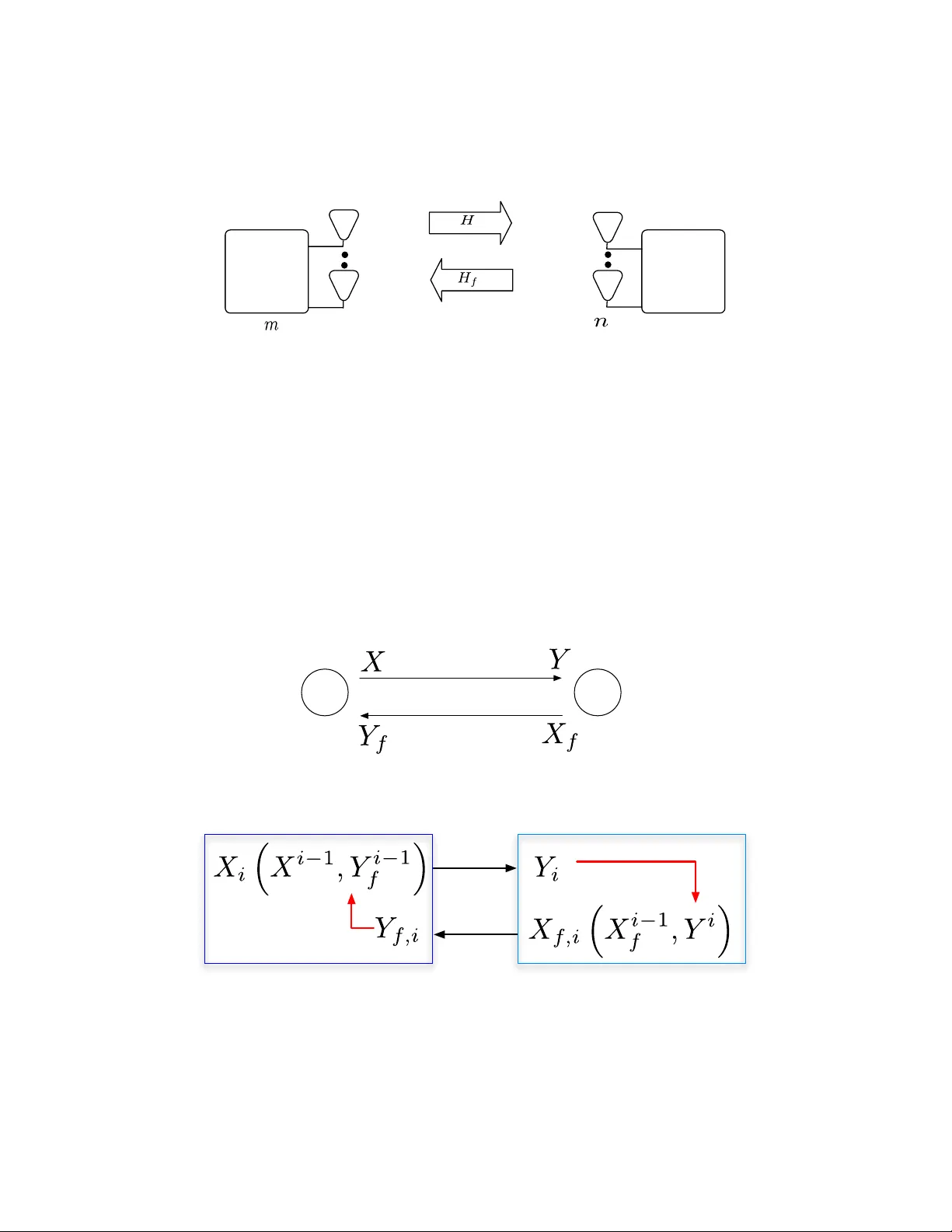
Comments & Academic Discussion
Loading comments...
Leave a Comment