Inference of Sparse Networks with Unobserved Variables. Application to Gene Regulatory Networks

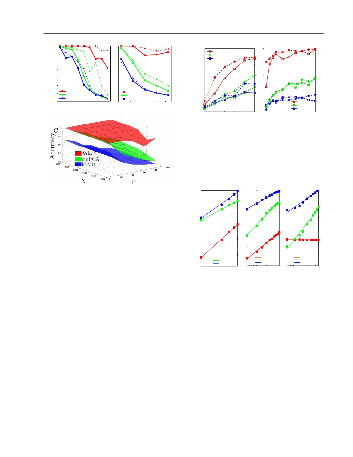
Inference of Sparse Net w orks with Unobserv ed V ariables. Application to Gene Regulatory Net w orks Nik olai Sla vo v Princeton Univ ersity , NJ 08544 nslavov@alum.mit.edu Abstract Net works are a unifying framew ork for mo d- eling complex systems and net work inference problems are frequen tly encoun tered in man y fields. Here, I dev elop and apply a generativ e approac h to net w ork inference ( RC web ) for the case when the net w ork is sparse and the laten t (not observed) v ariables affect the ob- serv ed ones. F rom all p ossible factor analysis (F A) decomp ositions explaining the v ariance in the data, RC web selects the F A decom- p osition that is consistent with a sparse un- derlying netw ork. The sparsity constraint is imp osed by a no vel metho d that significantly outp erforms (in terms of accuracy , robustness to noise, complexit y scaling and computa- tional efficiency) Ba yesian metho ds and MLE metho ds using ` 1 norm relaxation suc h as K– SVD and ` 1–based sparse principle comp o- nen t analysis (PCA). Results from simulated mo dels demonstrate that RC web reco vers ex- actly the mo del structures for sparsity as low (as non-sparse) as 50% and with ratio of un- observ ed to observed v ariables as high as 2. RC web is robust to noise, with gradual de- crease in the parameter ranges as the noise lev el increases. 1 In tro duction F actor analysis (F A) decomp ositions are useful for ex- plaining the v ariance of observ ed v ariables in terms of fewer unobserved v ariables that may capture sys- tematic effects and allow for low dimensional repre- sen tation of the data. Y et, the in terpretation of la- ten t v ariables inferred b y F A is fraugh t with problems. App earing in Pro ceedings of the 13 th In ternational Con- ference on Artificial Intelligence and Statistics (AIST A TS) 2010, Chia Laguna Resort, Sardinia, Italy . V olume 9 of JMLR: W&CP 9. Copyrigh t 2010 by the authors. In fact, in terpretation is not alwa ys exp ected and in- tended since F A may not hav e an underlying gener- ativ e mo del. A prime difficult y with interpretation arises from the fact that an y rotation of the factors and their loadings by an orthogonal matrix results in a dif- feren t F A decomp osition that explains the v ariance in the observed v ariables just as well. Therefore, in the absence of additional information on the latent v ari- ables and their loading, F A cannot identify a unique decomp osition, m uch less generativ e relationships b e- t ween latent factors and observed v ariables. A frequent choice for a constraint implemen ted by principle comp onent analysis (PCA) and resulting in a unique solution is that the factors are the singu- lar vectors (and thus orthogonal to each other) of the data matrix ordered in descending order of their corre- sp onding singular v alues. Y et, this choice is often mo- tiv ated b y computational conv enience rather than by kno wledge about the system that generated the data. Another type of computationally conv enien t constraint applied to facilitate the interpretation of F A results is sparsity , in the form of sparse Bay esian F A ( W est , 2002 ; Dueck et al , 2005 ; Carv alho and W est , 2008 ), sparse PCA ( d’Aspremont A , 2007 ; Sigg and Buh- mann , 2008 ) and F A for gene regulatory net works ( Sre- broand and Jaakkola , 2001 ; P e’er et al , 2002 ). Ho w- ev er, pap ers that introduce and use sparse PCA do not consider a generative mo del but rather use spar- sit y as a con venien t to ol to pro duce interpretable fac- tors that are linear com binations of just a few original v ariables. In sparse PCA, sparsit y is a wa y to balance in terpretability at the cost of slightly low er fraction of explained v ariance. The algorithm desc ribed in this pap er ( RC web ) also uses a sparse prior, but RC web explicitly considers the problem from a generative p erspective. RC web asserts that there is indeed a set of hidden v ariables that con- nect to and regulate the observed v ariables via a sparse net work. Based on that mo del, I derive a net work structure learning approach within explicit theoretical framew ork. This allows to prop ose an approach for sparse F A whic h is conceptually and computationally Inference of Sparse Net works with Unobserv ed V ariables. Application to Gene Regulatory Netw orks differen t from all existing approaches such as K-SVD ( Aharon et al , 2005 ), sparse PCA and other LARS ( Bradley et al , 2004 ) based metho ds ( Banerjee et al , 2007 ). RC web is appropriate for analyzing data arising from an y system in which the state of each observed v ariable is affected b y a strict subset of the unobserved v ariables. T o assign the inferred latent v ariables to ph ysical factors, RC web needs either data from p er- turbation exp eriments or prior knowledge ab out the factors. This framework generalizes to non-linear in- teractions, which is discussed elsewhere. F urthermore, I analyze the scaling of the computational complexity of RC web with the n um b er of observed and unobserv ed v ariables, as w ell as the parameter space where RC web can accurately infer netw ork top ologies and demon- strate its robustness to noise in the data. 2 Deriv ation Consider a sparse bipartite graph G = ( E , N , R ) con- sisting of tw o sets of vertices N and R and the asso- ciated set of directed edges E connecting R to N ver- tices. Define a graphical mo del in which each vertex s corresp onds to a random v ariable; N observed ran- dom v ariables indexed by N ( x N = { x s | s ∈ N } ) whose states are functions of P unobserved v ariables indexed b y R , x R = { x s | s ∈ R} . Since the states of x N dep end on (are regulated b y) x R , I will also refer to x R as reg- ulators. The functional dep endencies are denoted b y a set of directed edges E so that each unobserv ed v ariable x i | i ∈ R affects (and its vertex is th us connected to) a subset of observed v ariables x α i = { x s | s ∈ α i ⊂ N } . Giv en a dataset G ∈ R M × N of M configurations of the observed v ariables x N , RC web aims to infer the edges E and the corresp onding configurations of the unobserv ed v ariables, x R . If the state of each observed v ariable is a linear sup er- p osition of a subset of unobserved v ariables, the data G can b e modeled with a v ery simple gener ative mo del ( 1 ): The data is a pro duct b etw een R ∈ R M × P (a matrix whose columns corresp ond to the unobserved v ariables and the rows c orrespond to the M measured configurations) and C ∈ R P × N , the weigh ted adja- cency matrix of G . The unexplained v ariance in the data G is captured by the residual Υ . G = R C + Υ (1) This decomp osition of G into a pro duct of tw o matri- ces can b e considered to b e a t yp e of factor analysis with R b eing the factors and C the loadings. Ev en when P  M the decomp osition of G do es not hav e a unique solution since R C ≡ R I C ≡ RQ T QC ≡ R ∗ C ∗ for any orthonormal matrix Q . Th us the iden- tification of a unique decomp osition corresp onding to the structure of G requires additional criteria con- straining the decomp osition. The assumption that G is sparse requires that C b e sparse as well meaning that the state of the i th observ ed v ertex x i | i ∈ N is affected b y a strict subset of the unobserv ed v ariables x ψ i = { x s | s ∈ ψ i ⊂ R} , the ones whose weigh ts in the i th column of C are not zeros, C iψ i 6 = 0 and C i ¯ ψ i = 0 where ¯ ψ i is the complement of ψ i . Thus, to recov er the structure of G , RC web seeks to find a decomp osition of G in which C is sparse. The sparsity can b e intro- duced as a regularization with a Lagrangian m ultiplier λ : ( ˆ C , ˆ R ) = arg min R , C k G − R C k 2 F + λ k C k 0 (2) In the equations abov e and throughout the paper k C k 2 F = P i,j C 2 ij denotes en try-wise (F rob enius) norm, and the zero norm of a vector or matrix ( k C k 0 ) equals the n umber of non-zero elements in the array . T o infer the netw ork top ology RC web aims to solve the optimization problem defined by ( 2 ). Since ( 2 ) is a NP-hard com binatorial problem, the solution can b e simplified significan tly by relaxing the ` 0 norm to ` 1 norm ( Bradley et al , 2004 ). Then the approximated problem can b e tackled with interior p oint metho ds ( Banerjee et al , 2007 ). As an alternativ e approac h to ` 1 appro ximation, I prop ose a nov el metho d based on in tro ducing a degree of freedom in the singular-v alue decomp osition (SVD) of G by inserting an inv ertible 1 matrix B . G = USV T ≡  US ( B T ) − 1  | {z } ˆ R  B T V T  | {z } ˆ C (3) The prior (constrain t) that ˆ C is sparse determines B that minimizes ( 2 ), and th us a unique decomp osition. The goal of introducing B is to reduce the combina- torial problem to one that can b e solved with conv ex minimization. When the factors underlying the ob- serv ed v ariance are fewer than the observ ations in G there is no need to tak e the full SVD; if P factors are exp ected, only the first P largest singular vectors and v alues from the SVD of G are taken in that de- comp osition so that USV T is the matrix with rank P that b est approximates G in the sense of minimizing k G − USV T k 2 F . Since conceiv ably sparse decomp o- sitions may use columns outside of the best ` 2 ap- pro ximation, RC web considers taking the first P ∗ for P ∗ > P singular pairs. Suc h expanded basis is more lik ely to supp ort the optimal sparse solution and es- p ecially relev ant for the case when P is not known. Suc h c hoice can b e easily accommo dated in light of the ability of RC web to exclude unnecessary explana- tory v ariables, see section 4.3 . Next RC web computes B based on the requirement that C is sparse for the case N > P . T o compute 1 B is alwa ys inv ertible by construction, see section 4.3 and equation ( 4 ) Nik olai Sla vo v B , one may set an optimization problem ( 4 ). Once B is inferred, ˆ R and ˆ C can be computed easily , ˆ R = US ˆ B − 1 and ˆ C = ( V ˆ B ) T . ˆ B = arg min B k VB k 0 , so that det( B ) > 1 (4) The constraint on B in ( 4 ) is in tro duced to av oid trivial and degenerate solutions, suc h as B b eing rank defi- cien t B . Thus the introduction of B reduces ( 2 ) to a problem ( 4 ) that is still combinatorial and might also b e appro ximated with a more tractable problem b y re- laxing the ` 0 norm to ` 1 norm and applying heuristics ( Cetin et al , 2002 ; Cand` es et al , 2007 ) to enhance the solution. I prop ose a new approach, RC web , outlined in the next section. 3 RC web Assume that a sparse c T i corresp onding to an optimal ˆ b i (the i th column of ˆ B ) form V ˆ b i = c T i is known. Define the set of indices corresp onding to non-zero el- emen ts in c T i with ω − and the set of indices corre- sp onding to zero elements in c T i with ω 0 . F urthermore, define the matrix V ω 0 to be the matrix containing only the ro ws of V whose indices are in ω 0 . If ω 0 and th us V ω 0 are kno wn, one can easily compute ˆ b i as the righ t singular vector of V ω 0 corresp onding to the zero sin- gular v alue. Since c T i and ω 0 are not known, RC web appro ximates ˆ b i (the smallest 2 righ t singular v ector of V ω 0 ) with v s , the smallest right singular vector of V . This approximation relies on assuming that a low rank perturbation in a matrix results in a small change in its smallest singular vectors ( Wilkinson et al , 1965 ; Bena ych-Georges and Rao , 2009 ). Thus given that RC web is lo oking for the sparsest solution and the set ω − is small relative to N , the angle b etw een the sin- gular vectors of V ω 0 and V is small as well. There- fore, v s can serve as a reasonable first approximation of b i . Then RC web systematically and iterativ ely uses and up dates v s b y remo ving ro ws of V until v s con- v erges to b i or equiv alen tly V ω 0 b ecomes singular for the largest set of ω 0 indices. When V ω 0 b ecomes singu- lar, all elements of c i whose indices are in ω 0 b ecome zero. RC web also has an intuitiv e geometrical interpretation. Consider the matrix V mapping the unit sphere in R P (the sphere with unit radius from R P ) to an ellipsoid in R N . The axes of the ellipsoid are the left singular v ectors of V . In this picture, starting with ω − = {∅} and ω 0 = { 1 , . . . , N } , solving ( 4 ) requires moving the few est num b er of indices from ω 0 to ω − so that V ω 0 maps a vector from R P to the origin. How to choose 2 By smallest singular vector I mean the singular vector cor- responding to the to the smallest singular v alue the indices to b e mov ed? At each step RC web chooses i | max | , the index of the largest element (b y absolute v alue) of the smallest axis of the ellipsoid which is the left singular vector of V with the smallest singular v alue. RC web mo ves i | max | from ω 0 to ω − effectiv ely selecting the dimension whose pro jection is easiest to eliminate and removing its largest comp onent, which minimizes as muc h as p ossible the pro jection in that dimension. RC web keeps mo ving indices from ω 0 to ω − using the same pro cedure until the smallest right singular vector of V ω 0 con verges to b i and the small- est singular v alue of V ω 0 approac hes zero. RC web is guaran teed to stop after at most ( N − P + 1) steps since after remo v al of ( N − P + 1) indices from ω 0 , V ω 0 will b e at most rank P − 1. If RC web finds a sparse solution it will con verge in fewer steps. 1. T ask: ˆ b i = min b T i b i ≥ 1 k Vb i k 0 2. Initialization: • ω − = {∅} and ω 0 = { 1 , 2 , . . . , N } • Set K − 1 ω 0 = ( V T ω 0 V ω 0 ) − 1 = I ∈ R P × P • Set J = 1; • i | max | = arg max  P j | V ij |  ω − = { i | max | } , ω 0 = { i | i ∈ ω 0 , i 6 = i | max | } • Up date K − 1 ω 0 = Rank U pdate ( K − 1 ω 0 , V i | max | ) 3. Cycle: J = J + 1 Rep eat until conv ergence • Find the eigenv ector v for K − 1 ω 0 with the largest eigen v alue λ max • If λ − 1 max ≈ 0 or v J → v J − 1 , ˆ b i ≡ v ; STOP • Compute the left singular vector of V ω 0 u = s − 1 V ω 0 v • i | max | = arg max [( | u 1 | , . . . , | u i | , . . . , | u N | )]; • ω − = { ω − , i | max | } ω 0 = { i | i ∈ ω 0 , i 6 = i | max | } • Up date K − 1 ω 0 = Rank U pdate ( K − 1 ω 0 , V i | max | ) The ab o ve algorithm can compute a single vector, ˆ b i , whic h is just one column of ˆ B . T o find the other columns, RC web applies the same approach to the mo dified (inflated) matrix, which for the i th column of B is V ( i ) = V ( i − 1) + V ˆ b i ˆ b T i for i = 2 , . . . , P . Thus, after the inference of eac h column of B RC web mo di- fies V ( i − 1) to V ( i ) ( V (1) ≡ V ) so that the algorithm will not replicate its c hoice of ω 0 . Note that in the i th up date of V ( i − 1) the V ˆ b i ˆ b T i will modify only the ω − ro ws in V ( i − 1) since the rows of the V ˆ b i ˆ b T i whose indices are in ω 0 con tain only zero elements. Apply- ing RC web to the inflated matrices av oids inferring Inference of Sparse Net works with Unobserv ed V ariables. Application to Gene Regulatory Netw orks m ultiple times the same ˆ b i , but a ˆ b i inferred from the inflated matrix is generally going to differ at least sligh tly from the corresponding ˆ b i that solves ( 4 ) for V . T o av oid that, RC web uses the inflated matrices only for the first few iterations until the largest (by absolute magnitude) of the Pearson correlations b e- t ween the smallest eigenv ector of V ω 0 from the current ( i th ) iteration and the reco vered columns of B is less than 1 −  and monotonically decreasing;  is chosen for numerical stability and also to reflect the similar- it y b etw een the connectivity of R vertices that can b e exp ected in the netw ork whose top ology is b eing reco vered. A simpler alternativ e that works great in practice is to use the the inflated matrix for the first k iterations that are enough to find a new direction for ˆ b i and then RC web switches back to V so that the solution is optimal for V . The switch requires k rank up date of K − 1 ω 0 ≡ ( V T ω 0 V ω 0 ) − 1 and thus choosing k small sav es computations. Cho osing k to o small, how- ev er, ma y not b e enough to guarantee that ˆ b i will not recapitulate a solution that is already found. Usually k = 10 w orks great and can be easily increased if the new solution is v ery close to an old one. There are a few notable elements that mak e RC web efficien t. First, RC web do es almost all computations in R P and since P  N , P < M , that sav es b oth memory and CPU time. Second, eac h step requires only a few matrix-vector multiplication for computing the eigenv ectors (since the change from the previous step is generally very small) and K − 1 ω 0 is computed b y a rank–one up date whic h obviates matrix inv ersion. The approach that RC web takes in solving ( 4 ) do es not imp ose sp ecific restrictions on the distribution of the observed v ariables ( G ), the noise in the data ( Υ ) or the latent v ariables ˆ R . How ev er, the initial approx- imation of b i with v s can be p o or for data arising from dense net works or sp ecial worst–case datasets. As demonstrated theoretically (Bena ych-Georges 2009) and tested n umerically in the next section, RC web per- forms v ery well at least in the absence of worst–case scenario sp ecial structures in the data. 4 V alidation T o ev aluate the p erformance of RC web , I first apply it to data from sim ulated random bipartite netw orks with t wo different top ology types, (1) Erd¨ os & R` en yi and (2) scale-free whose corresp onding degree distribu- tions are (1) P oisson and (2) p ow er–la w. The net work top ology is enco ded in a weigh ted adjacency matrix C g old and the v alues for the unobserv ed v ariables are dra wn from a standard uniform distribu tion. The sim- ulations result in data matrices G ∈ R M × N con taining M observ ations of all N unobserved v ariables. Accord- ing to RC web , the optimal sparse adjacency matrix ( ˆ C ) and the hidden v ariables ( ˆ R ) can b e inferred by the decomp osition, ˆ G = ˆ R ˆ C so that ˆ C is as sparse as p ossible while ˆ G is as close as p ossible to G . In addition to RC web , suc h decomposition can b e com- puted b y 3 classes of existing algorithms. F or a com- parison, I use the latest v ersions for which the authors rep ort b est p erformance: ( A ) PSMF for Bay esian ma- trix factorization as implemen ted b y the author Mat- Lab function PSMF1 ( Dueck et al , 2005 ); ( B ) BFRM 2 for Ba yesian matrix factorization as implemen ted b y the author compiled executable ( Carv alho and W est , 2008 ); ( C ) emPCA for maxim um likelihoo d estimate ( MLE ) sparse PCA ( Sigg and Buhmann , 2008 ); ( D ) K-SVD ( Aharon et al , 2005 ). All algorithms are im- plemen ted using the code published by their authors, and with the default v alues of the parameters when parameters are required. The results are compared for v arious M, N, P , sparsit y , and noise levels. 4.1 Limitations Before comparing the results, consider some of the lim- itations common to all algorithms and the appropriate metrics for comparing the results. In the absence of an y other information, the decomposition of G (no matter how accurate) cannot asso ciate hidden v ari- ables (corresp onding to columns of ˆ R ) to physical fac- tors. F urthermore, all metho ds can infer ˆ C and ˆ R only up to an arbitrary diagonal scaling or p ermuta- tion matrix. First consider the scaling illustrated by the following transformation by a diagonal matrix D , ˆ G = ˆ R ˆ C = ˆ R I ˆ C = ˆ R ( DD − 1 ) ˆ C = ( ˆ RD )( D − 1 ˆ C ) = ˆ R ∗ ˆ C ∗ . Suc h transformation is going to rescale ˆ R to ˆ R ∗ and ˆ C to ˆ C ∗ , which is just as sparse as ˆ C , k ˆ C ∗ k 0 = k ˆ C k 0 . Since b oth decomp ositions explain the v ariance in G equally w ell RC web (or any of the other metho d) cannot distinguish b etw een them. Thus giv en ˆ C , there is a diagonal matrix ˆ D that scales ˆ C to C g old , the w eighted adjacency matrix of G . The second limitation is that in the absence of addi- tion information, RC web can determine ˆ C and R up to a p erm utation matrix. Consider comparing ˆ C to the adjacency matrix used in the simulations, C g old . Since the identit y of the inferred hidden v ariables is not known the rows of ˆ C do not generally correspond to the rows of C g old ; ˆ C i (the i th ro w of ˆ C ) is most lik ely to corresp ond to the C g old ro w that is most cor- related to ˆ C i and the Pearson correlation b etw een the t wo rows quan tifies the accuracy for the inference of ˆ C i . T o implement this idea, all ro ws of ˆ C and C g old are first normalized to mean zero and unit v ariance resulting in C nor and C g old nor . The correlation matrix then is, Σ = C T nor C g old nor and the most likely v ertex (index of the unobserv ed v ariable) corresp onding to ˆ C i is k = arg max j ( | Σ i 1 | , . . . , | Σ ij | , . . . , | Σ iP | ), where Nik olai Sla vo v k ∈ R . The absolute v alue is required b ecause the di- agonal elements of ˆ D can b e negative. The accuracy is measured by the corresp onding P earson correlation, ρ i = | Σ ik | . An optimal solution of this matching prob- lem can b e found by using b elief propagation algorithm for the simple case of a bipartite graph even the LP relaxed v ersion guarantees optimal solution (Sanghavi 2007). The ov erall accuracy is quantified b y the mean correlation ¯ ρ = (1 /p ) P i = p i =1 ρ i where p is the num ber of inferred unobserv ed v ariables and can equal to P or not dep ending on whether the n umber of unobserv ed v ariables is kno wn or not. In computing ¯ ρ , each row of C g old is allow ed to corresp ond only to one row of ˆ C and vice v ersa. In addition to the t wo common limitations of p ermu- tation and scaling, some algorithms ( d’Aspremont A , 2007 ) for sparse PCA require M > N and since this is not the case in many real world problems and in some of the datasets simulated here, those metho ds are not tested. Instead I chose emPCA, which do es not require M > N and is the latest MLE algorithm for sparse PCA that according to its authors is more efficien t than previous algorithms ( Sigg and Buhmann , 2008 ). 4.2 Accuracy and complexit y scaling RC web has a natural wa y for iden tifying the mean de- gree 3 . How ever, some of the other algorithms require the mean degree for optimal p erformance. T o av oid underestimating an algorithm simply b ecause it reco v- ers netw orks that are to o sparse or not sparse enough, I assume that the mean degree is known and it is in- put to all algorithms. First all algorithms are tested on a v ery easy inference problem, Fig.1. Since PSMF and BFRM hav e low er accuracy and PSMF is signif- ican tly slo wer than the other algorithms, the rest of the results will fo cus on the MLE algorithms that also ha ve b etter p erformance. PSMF gives less accurate results with p ow er–la w netw orks which can b e under- sto od in terms of the uniform prior used by PSMF. PSMF has the adv antage ov er the MLE algorithms in inferring a probabilistic netw ork structure rather than a single estimate. Sp ecial adv an tage of BFRM is the seamless inclusion of resp onse v ariables and measured factors in the inference. F or the MLE algorithms, the accuracy of netw ork inference increases with the ra- tio of observed to unobserved v ariables N /P (Fig.2) and with the num ber of observ ed configurations M , Fig.3. In contrast, as the noise in the data and the mean out–degree (mean num ber of edges from R to N v ertices) are increased, the accuracy of the inference decreases. All algorithms p erform b etter on P oisson 3 When RC web learns all edges, the smallest singular v alue of V ω 0 approaches zero and its smallest singular vector conv erges to ˆ b i . 10 15 20 25 30 35 40 45 50 55 60 0 0.2 0.4 0.6 0.8 1.0 Num be r of unob served var i ables, P Inference Accuraccy , ¯ ρ RC we b emPC A kSVD PS MF BFRM Figure 1: Accuracy of netw ork recov ery as a function of the num b er of unobserved v ariables, P . Num b er of observed v ariables N = 500; Number of observ a- tions, M = 280. All netw orks are with P oisson mean out–degree 0 . 10 N = 50, with 10 % noise in the obser- v ations. net works and the low er level of noise in the data from p o wer–la w netw orks was c hosen to partially comp en- sate for that. An imp ortant cav eat when comparing the results for different algorithms is that K-SVD it- erativ ely improv es the accuracy of the solution, and th us the output is dep enden t on the maximum num- b er of iterations allow ed ( I max ). F or the results here, I max = 20 and the accuracy of K-SVD ma y improv e with higher num ber of iterations ev en though I did not observe significant improv emen t with I max = 100. Ev en at 20 iterations K-SVD is significan tly slow er than RC web and emPCA, Fig.4. The scaling of the al- gorithms with resp ect to a parameter was determined b y holding all other parameters constant and regress- ing the log of the CPU time against the log of the v ariable parameter, Fig.4. The scaling with resp ect to some parameters is b elow the theoretical exp ecta- tion since the highest complexity steps may not b e sp eed–limiting for the ranges of parameters used in the sim ulations. 4.3 In terpretability In analyzing real data the num b er of unobserved v ari- ables ( P ) may not b e kno wn. I observe that if a sim- ulated netw ork having P regulators is inferred assum- ing P ∗ > P regulators, the elements of B corresp ond- ing to the excessive regulators are very close to zero, | B ij | ≤ 10 − 10 for i > P or j > P . Thus, if the data truly originate from a sparse netw ork RC web can dis- card unnecessary unobserv ed v ariables. The results of RC web can b e v aluable even without iden tifying the physical factors corresp onding to x R . Y et identifying this corresp ondence, and thus ov er- coming the limitations outlined in section 4.1 can b e Inference of Sparse Net works with Unobserv ed V ariables. Application to Gene Regulatory Netw orks 0 20 40 60 80 0.4 0.5 0.6 0.7 0.8 0.9 1 Number o f uno bs erved v ar ia bl es, P Infer ence Acc ura ccy , ¯ ρ A RC web emPCA kSVD 0 20 40 60 80 0.2 0.3 0.4 0.5 0.6 0.7 0.8 0.9 1 RC web emPCA kSVD B Figure 2: Accuracy of net work recov ery as a function of the num b er of unobserved v ariables, P . The thic ker brigh ter lines with squares corresp ond to num ber of observ ed v ariables N = 500 and the dashed, thinner lines corresp ond to N = 1000. In all cases the num ber of observ ations is M = 2000. A) Poisson netw orks with mean out–degree 0 . 25 N { 125 and 250 } , with 50 % noise in the observ ations and B) p o wer–la w netw orks (with mean out–degree 0 . 40 N { 200 and 400 } , with 10 % noise in the observ ations. C) The same as (B) except for wider range of the observ ed v ariables. v ery desirable. One practically relev ant situation al- lo wing in-depth interpretation of the results requires measuring (if only in a few configurations) the states of some of the v ariables that are generally unobserved ( x R ). This is relev ant, for example, to situations in whic h measuring some v ariables is m uch more exp en- siv e than others (such as protein modifications v ersus messenger RNA concentrations) and some x s ∈R can b e observ ed only once or a few times. Assume that the states of the k th ph ysical factor are measured (data in v ector u k ) in n k n umber of configurations, whose in- dices are in the set φ k . This information can be enough for determining the vertex x s ∈R corresp onding to the k th factor and the corresp onding ˆ D ss as follows: 1) Compute the Pearson correlations ~ ρ b et ween u k and the columns of ˆ R φ k . Then, the vertex of the inferred net work most likely to corresp ond to the k th ph ysi- cal factor is s = arg max i ( | ρ 1 | , . . . , | ρ i | , . . . , | ρ P | ). 2) ˆ D ss = ( ˆ R T φ k ˆ R φ k ) − 1 ˆ R T φ k u k . Similar to section ( 4.1 ), w eighted matching algorithms (Sanghavi 2007) can b e used for finding the optimal solution if there is data 0 200 400 600 800 0.4 0.5 0.6 0.7 0.8 0.9 1 B RC web emPCA kSVD 50 100 150 200 250 300 0.2 0.3 0.4 0.5 0.6 0.7 0.8 0.9 1 Infer ence Ac cura ccy , ¯ ρ A RC web emPCA kSVD Number of O bser ved Config ur at io ns , M Figure 3: Accuracy of net work recov ery as a function of the num b er of observ ed configurations, M . Contin- uous lines & squares, N = 500; dashed lines & circles, N = 1000 A) Poisson net works with mean out–degree 0 . 20 N { 100 and 200 } , with 50 % noise; B) p ow er–la w net works (with mean out–degree 0 . 40 N { 200 and 400 } , with 10 % noise. In all cases P = 30. 10 1 10 0 10 1 10 2 10 3 10 4 10 5 P CPU Tim e, secon d s A RC web : 1.78 emPCA: 1.03 kSVD: 1.40 10 3 10 1 10 2 10 3 10 4 10 5 N B RC web : 1.41 emPCA: 1.80 kSVD: 0.98 10 2 10 0 10 1 10 2 10 3 M C RC web : -0.01 emPCA: 1.33 kSVD: 0.73 Figure 4: Computational efficiency as a function of P , M and N . The scaling exp onents (slopes in log–log space) are rep orted in the legends. The netw orks are with p ow er–la w degree distribution and 60 % sparsity , with mean out–degree 0.40N for m ultiple x s ∈R . P artial prior knowledge ab out the structure of G can also b e used to enhance the interpretabilit y of RC web results. Assume, for example, that some of the no des ( x s ∈ α k ⊂N ) regulated by the k th ph ysical factor (which is a hidden v ariable in the inference) are known. Then the matc hing approac h that was just outlined can b e used with ˆ C rather than ˆ R . If the w eights are not known all non-zero elements of ˆ C α k can b e set to one. The significance of the o verlap (fraction of common edges) of the regulator most lik ely to corre- sp ond to the k th ph ysical and its kno wn connectiv- it y (coming from prior knowledge) can b e quantified b y a p-v al (the probability of observing such o verlap Nik olai Sla vo v b y chance alone) computed from the h yp er–geometric distribution. This approac h is exemplified with gene- expression data in the next section. 4.4 Application to data Sim ulated mo dels ha v e the adv an tage of ha ving kno wn top ology , and thus providing excellent basis for rig- orous ev aluation. Suc h rigorous ev aluation is not p ossible for real biological netw orks. Y et, existing partial knowledge of transcriptional net works, can b e combined with the approac h outlined in section 4.3 for ev aluation of inference of biological netw orks. In particular, consider the transcriptional net work of budding yeast, Saccharom yces c er evisiae . It can b e mo deled as a tw o-la yer netw ork with transcription factors (TFs) and their complexes b eing regulators ( x R ) whose activities cannot b e measured on a high- throughput scale because of technology limitations. TFs regulate the expression levels of messenger RNAs (mRNAs) whose concen trations can b e measured eas- ily on a high-throughput scale at multiple physiolog- ical states and represent the observed v ariables, x N . A partial kno wledge ab out the connectivit y in this transcriptional netw ork comes from ChIP-chip exp er- imen ts ( MacIsaac , 2006 ) which identify sets of genes regulated b y the same transcription factors (TFs). I first apply RC web to a set mRNA configurations fol- lo wed b y the approach of section 4.3 to ev aluate the results. The data matrix G contains 423 yeast datasets measured on the Affymetrix S98 microarra y platform at a v ariet y of ph ysiological conditions. RC web was initialized with P ∗ = 160 unobserved v ariables (corre- sp onding to TFs) and identified P = 153 co-regulated sets of genes. The inferred adjacency matrix ˆ C is com- pared directly to the adjacency matrix identified by ChIP-c hip exp eriments ( MacIsaac , 2006 ). Indeed, sets of genes inferred by RC web to b e co-regulated o ver- lap substan tially with sets of genes found to b e reg- ulated by the same TF in ChIP-chip studies, Fig.5. F urthermore, the most enriched gene on tology (GO) terms associated with the RC web inferred sets of genes corresp ond to the functions of the resp ective TFs. This fact provides further supp ort to the accuracy of the inferred netw ork top ology and suggests that man y of the genes inferred to be regulated b y the corresp onding TFs ma y be b ona fide targets that w ere not detected in the ChIP-chip exp erimen ts because of the rather lim- ited set of physiological conditions in which the exp er- imen ts are performed ( MacIsaac , 2006 ). Since the best “gold standard” is the only partially known top ology , comparing the p erformance of the different algorithms in this setting can b e hard to interpret; an algorithm can b e p enalized for correctly inferred edges if these edges are absen t from the incomplete ChIP top ology . An ob jectiv e comparison requires exp erimental test- Figure 5: Overlap b etw een the first 7 sets of genes (column 1) that RC web identifies to b e regulated by a common regulator and sets of genes whose promoters are b ound by the same TF (column 2) in ChIP-chip exp erimen ts. The second and third columns list the n umber of ov erlapping genes b etw een the RC web set and the ChIP-c hip set and the corresponding probabil- ities of observing such ov erlaps b y chance alone. The fourth column contains a description of the TFs from the second column and the fifth column lists the most enric hed GO terms for the RC web gene sets. ing of predicted new edges and that is the sub ject of a forthcoming pap er. The comparison b et ween ChIP–chip gene sets and RC web gene sets allows to iden tify the lik ely corre- sp ondences b etw een x s ∈R and TFs and to infer the activities of the TFs which are very hard to mea- sure exp erimentally but crucially imp ortant to under- standing the dynamics and logic of gene regulatory net works ( Slav ov and Dawson , 2009 ; Silverman et al , 2010 ; Sla vo v , 2010 ). 5 Conclusions This pap er introduces an approach ( RC web ) for in- ferring latent (unobserv ed) factors explaining the b e- ha vior of observed v ariables. RC web aims at inferring a sparse bipartite graph in whic h vertices connect in- ferred latent factors (e.g. regulators of mRNA tran- scription and degradation) to observ ed v ariables (e.g. target mRNAs). The salien t difference distinguishing RC web from prior related w ork is a new approach to attaining sparse solution that allo ws the natural inclu- sion of a generativ e mo del, relaxation of assumptions on distributions, and ultimately results in more accu- rate and computationally efficien t inference compared to comp eting algorithms for sparse data decomp osi- tion. Ac knowledgmen ts I thank Dmitry Malioutov and Ro dolfo Ros Zertuche for many insightful discussions and extensive, con- structiv e feedback, as w ell as David M. Blei, David Inference of Sparse Net works with Unobserv ed V ariables. Application to Gene Regulatory Netw orks Botstein and Kenneth A. Dawson for supp ort and commen ts. This work was supp orted by Irish Re- searc h Council for Science, Engineering and T ec hnol- ogy (IRCSET) and by Science F oundation Ireland un- der Gran t No.[SFI/SRC/B1155]. References Aharon M, Elad M, Bruckstein AM (2005) K-SVD and its non-negative v ariant for dictionary design. Wavelets XI 5914 : 591411–591424 Banerjee O, Ghaoui L, d’Aspremont. A (2007) Mo del selection through sparse maximum likelihoo d esti- mation. JMLR 9 : 485–516 Bena ych-Georges F, Rao R (2009) The eigen v alues and eigen vectors of finite, lo w rank p erturbations of large random matrices. arXiv09102120v1 Bradley E, T revor H, Iain J, Tibshirani R (2004) Least Angle Regression. A nnals of Statistics 32 : 407–499 Cand ` es E, W akin M, Boyd S (2007) Enhancing spar- sit y b y rew eighted ` 1 minimization. J F ourier Anal Appl 14 : 877–905 Carv alho C, W est M (2008) High-dimensional sparse factor mo delling: Applications in gene expression genomics. JASA 103 : 1438–1456 Cetin M, Maliouto v D, Willsky A (2002) A V aria- tional T echnique for Source Localization based on a Sparse Signal Reconstruction P ersp ective. ICASSP Orlando Florida 3 : 2965–2968 d’Aspremon t A Bach F. GL (2007) Optimal Solutions for Sparse Principal Comp onent Analysis. JMLR 9 : 1269–1294 Duec k D, Morris Q, F rey B (2005) Multi-wa y clus- tering of microarra y data using probabilistic sparse matrix factorization. Bioinformatics 21 : 144–151 MacIsaac K (2006) An improv ed map of conserv ed regulatory sites for Saccharom yces cerevisiae. BMC Bioinformatics 7 : 877–905 P e’er D, Regev A, T anay A (2002) Minreg: Inferring an activ e regulator set. Bioinformatics 18 : 258–267 Sigg C, Buhmann J (2008) Exp ectation-Maximization for Sparse and Non-Negativ e PCA. ICML Helsinki Finland 9 Silv erman S, Petti A, Sla vo v N, Parsons L, Briehof R, Thib erge S, Zenklusen D, Gandhi S, Larson D, Singer R, et al (2010) Metab olic cycling in single y east cells from unsynchronized steady-state p opu- lations limited on glucose or phosphate. Pr o c e e dings of the National A c ademy of Scienc es 107 : 6946– 6951 Sla vo v N (2010) Universality, sp e cificity and r e gulation of S. c er evisiae gr owth r ate r esp onse in differ ent c ar- b on sour c es and nutrient limitations . Ph.D. thesis, Princeton Univ ersity Sla vo v N, Dawson KA (2009) Correlation signature of the macroscopic states of the gene regulatory net- w ork in cancer. Pr o c e e dings of the National A c ademy of Scienc es 106 : 4079–4084 Srebroand N, Jaakkola T (2001) Sparse Matrix F ac- torization for Analyzing Gene Expression P atterns. NIPS 9 W est M (2002) Bay esian factor regression mo dels in the large p , small n paradigm. Bayesian Stat 7 : 723– 732 Wilkinson JH, Wilkinson JH, Wilkinson JH (1965) The algebr aic eigenvalue pr oblem . volume 87. Ox- ford Univ Press