ExpertBayes: Automatically refining manually built Bayesian networks

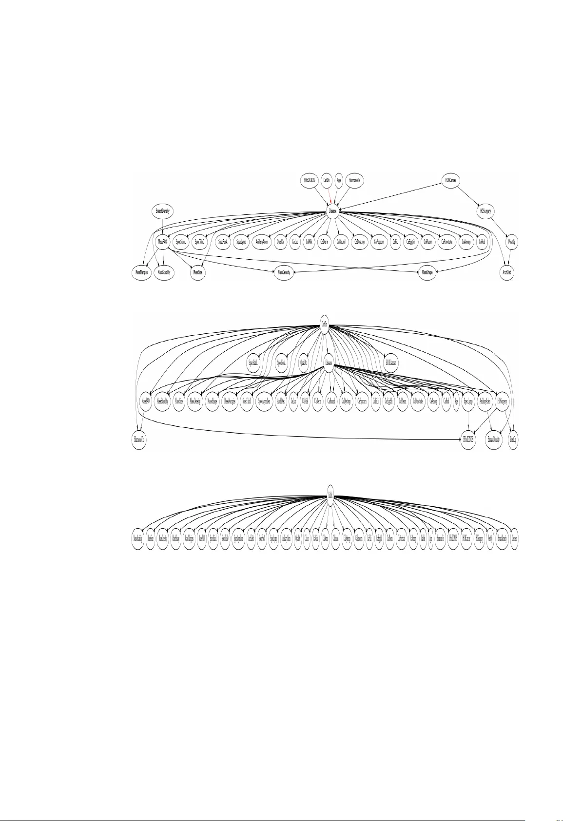
ExpertBayes: A utomatically r efining manually b uilt Bayesian netw orks Ezilda Almeida 1 , Pedro Ferreira 2 , T iago V inhoza 3 , In ˆ es Dutra 2 Jingwei Li 4 , Y irong W u 4 , and Elizabeth Burnside 4 1 CRA CS INESC TEC LA, 2 Department of Computer Science, Univ ersity of Porto 3 Instituto de T elecommunicac ¸ ˜ oes, IT -Porto 4 Univ ersity of Wisconsin, Madison, USA Abstract. Bayesian network structures are usually built using only the data and starting from an empty network or from a na ¨ ıve Bayes structure. V ery often, in some domains, like medicine, a prior structure knowledge is already known. This structure can be automatically or manually refined in search for better perfor- mance models. In this work, we take Bayesian networks built by specialists and show that minor perturbations to this original network can yield better classifiers with a very small computational cost, while maintaining most of the intended meaning of the original model. Keyw ords: bayesian networks, advice-based systems, learning bayesian network structures 1 Introduction Bayesian networks are directed acyclic graphs that represent dependencies between variables in probabilistic models. In these networks, each node represents a variable of interest and the edges may represent causal dependencies between these variables. A Bayesian network encodes the Marko v assumption that each variable is independent of its non-descendants, gi ven just its parents. Each node (variable) is associated with a conditional probability table. When used for knowledge representation, a network is simply a graphical model that represents relations among variables. This graphical model can be learned from data or can be manually built. In the latter case, the network encodes the knowledge of an expert and can serve as a basis for the construction of new networks. When learned only from data, the final graphical model (network structure) may not have a meaning for a specialist in the domain defined by the data. In this work, we aim to gather the advantages of manual construction with the ad- vantages of automatic construction, using ExpertBayes, a system that implements an algorithm that can refine pre viously built networks. ExpertBayes allows for (1) reduc- ing the computational costs inv olved in building a network only from the data, (2) em- bedding knowledge of an expert in the newly built network and (3) manual building of fresh new graphical representations. The main ExpertBayes algorithm is random and 2 Almeida et al. implements 3 operators: insertion, remov al and reversal of edges. In all cases, nodes are also chosen randomly . Our expert domains are prostate cancer and breast cancer . W e used graphical models manually built by specialists as starting networks. Parameters are learned from the data, but can also be giv en by the specialists. W e compare the performance of our original networks with the best network found using our random algorithm. Results are v alidated using 5-fold cross-validation. For dif ferent threshold v alues, results, both in the training and test sets, show that there is a statistically significant difference between the original network and the newly b uilt networks. As far as we know , this is the first implementation of an algorithm capable of constructing Bayesian networks from prior kno wledge in the form of a netw ork structure. Previous works considered as initial network a na ¨ ıve Bayes or an empty network [10,12,14,5]. As far as we kno w , the R package deal [2] is the only one that refines pre vious Bayesian structures, but our attempts to make it work were not successful, since the parameters computed for the new networks were not interpretable. W e then decided to implement our own algorithm. One important aspect of ExpertBayes is that it makes small perturbations to the original model thus maintaining its intended meaning. Besides refining pre-defined net- works, ExpertBayes is interactive. It allo ws users to play with the network structure which is an important step in the inte gration of expert kno wledge to the automatic lea rn- ing process. 2 ExpertBayes: r efining expert-based Bayesian networks Most works in the literature that discuss methods for learning the structure of Bayesian networks focus on learning from an empty network or from data. Ho wev er , in some do- mains, it is common to find Bayesian models manually b uilt by experts, using tools such as GeNIe (a modeling en vironment dev eloped by the Decision Systems Laboratory of the Uni versity of Pittsb urgh, a vailable at http://genie.sis.pitt.edu ), Netica ( https://www.norsys.com/netica.html ) or the WEKA Bayes editor [10]. Having an initial model brings at least two advantages: (1) from the point of view of the specialist, some expert knowledge has already being embedded to the model, with meaningful correlations among variables, (2) from the point of view of the structure learning algorithm, the search becomes less costly , since an initial structure is already known. In fact, in other areas, it is very common to use pre vious knowledge to reduce the search space for solutions. One classical e xample is the comb-like structure used as initial seed for DN A reconstruction algorithms based on Steiner minimum trees. In the past, the protein structure was searched for from an empty initial structure [15]. The discov ery that most protein structures in the nature had a comb-like shape reduced the algorithm cost allowing to solv e much bigger problems [11]. ExpertBayes uses a simple, yet ef ficient algorithm to refine the original network. This algorithm is sho wn in Figure 20. It reads the initial input network and training and test sets. It then uses a standard method to initialize the probability tables, by counting the case frequency of the training set for each table entry . Ha ving the prior network and conditional probability tables, the algorithm makes small perturbations to the original model. It first chooses a pair of nodes, then it randomly chooses to add, remo ve or revert ExpertBayes 3 an edge. If the operation is to add an edge, it will randomly choose the edge direction. Operations are applied if no c ycle is produced. At each of these steps, conditional prob- ability tables are updated, if necessary , i.e., if any node affected belongs to the Markov blanket of the classifier node. A score of the ne w model is calculated for the training set and only the best pair network/score is retained when the repeat cycle ends. This best network is then applied to the test set (last step, line 20 of the algorithm). A global score metrics is used, the number of correctly classified instances, according to a threshold of 0.5. Data : OriginalNet, // initial network structure ; T rain // training set ; T est // test set Result : scoreT rain // scor es in the training set for BestNet scoreT est // scor es in the test set for BestNet BestNet // best scor ed network on T rain 1 Read OriginalNet; 2 Read T rain and T est sets; 3 BestNet = OriginalNet; 4 Learn parameters for OriginalNet from training set; 5 repeat 6 Randomly choose a pair of nodes N 1 and N 2 ; 7 if ther e exists an edge between N 1 and N 2 then 8 randomly choose: rev ert or remove 9 else 10 choose add operation; 11 randomly choose edge direction 12 end 13 Apply operation to OriginalNet obtaining NewNet; 14 Rebuild necessary CPT entries, if necessary; 15 Compute scoreT rain of the NewNet; 16 if scor eT rain NewNet > scoreT rain BestNet then 17 BestNet = NewNet 18 end 19 until N iterations using OriginalNet and T rain ; 20 Apply BestNet to T est and compute scoreT est; Algorithm 1: ExpertBayes The modifications performed by ExpertBayes are always ov er the original netw ork. This was strategically chosen in order to cause a minimum interference on the expert knowledge represented in the graphical model. ExpertBayes has also the capability of creating a new netw ork only from the data if the user has no initial network to provide. 4 Almeida et al. 3 Materials and Methods The manual construction of a Bayesian network can be tedious and time-consuming. Howe ver , the knowledge encoded in the graphical model and possibly in the prior prob- abilities is very valuable. W e are lucky enough to ha ve two of these networks. One w as built for the domain of prostate cancer and the second one w as built for breast cancer . In the prostate cancer domain, variables were collected [13] taking into account three different moments in time: (1) during a medical appointment, (2) after auxiliary exams are performed and (3) five years after a radical prostatectomy . Such v ariables are age, weight, family history , systolic and diastolic arterial blood pressure, hemoglobin rate, hypoecogenic nodules, prostate specific-antigen (psa), clinical status, doubling time PSA, prostate size, among others. Five years after the sur gery , we assess morbidity for those patients. The data for breast cancer was collected from patients of the Univ ersity of W is- consin Medical Hospital. Mammography features were annotated according to the BI- RADS (Breast Imaging and Data Reporting System) [4]. These include breast density , mass density , presence of mass or calcifications and their types, architectural distortion, among others. One variable indicates the diagnostic and can have values malignant or benign, to indicate the type of finding. A third set of data w as used, also with mammographic features from the Uni versity of Wisconsin Medical Hospital, but with a dif ferent set of patients and a smaller number of variables. 3.1 Original Bayesian Networks T wo of our networks were built by specialists while the third one was built by us. The Bayesian networks b uilt by our specialists are shown in Figures 1 [13] and 2 [3]. Fig. 1: Original Network Model for Prostate Cancer W e call them Original Networks. Both of them were built by specialists in prostate cancer and breast cancer using high risk and lo w risk f actors mentioned in the literature ExpertBayes 5 Fig. 2: Original Network Model for Breast Cancer (1) Fig. 3: Original Network Model for Breast Cancer (2) and their o wn experience. Prior probabilities are taken from the training data. The class variable for the breast cancer data is CatDx. In other words, the classifying task is to predict a malignant or benign finding. The class v ariable for the prostate cancer data is the life expectanc y five years after the sur gery , called class in Figure 1. The third network was also manually b uilt using the model of Figure 2 as a basis, b ut with a smaller set of features used in another work [8]. The class variable is Outcome with values malignant or benign. 3.2 Datasets The characteristics of the datasets used are shown in T able 1. The three of them have only two classes. F or Breast Cancer (1) and Breast Cancer (2), the Pos column indicates the number of malignant cases and the Neg column indicates the number of benign cases. F or Prostate Cancer , the Pos column indicates the number of patients that did not surviv e 5 years after surgery . The dataset for Prostate Cancer is a vailable from http://lib.stat.cmu. edu/S/Harrell/data/descriptions/prostate.html [1]. For each one of the datasets, variables with numerical values were discretized ac- cording to reference values in the domain (for example, variables such as age and size are discretized in interv als with a clinical meaning). The same discretized datasets were used with all algorithms. 6 Almeida et al. Dataset Number of Instances Number of V ariables Pos Neg Prostate Cancer 496 11 352 144 Breast Cancer (1) 100 34 55 45 Breast Cancer (2) 241 8 88 153 T able 1: Datasets Descriptions 3.3 Methodology W e used 5-fold cross-v alidation to train and test our models. W e compared the score of the original network with the score of ExpertBayes. W e also used WEKA [10] to build the network structure from the data with the K2 [7] and T AN [9] algorithms. K2 is a greedy algorithm that, given an upper bound to the number of parents for a node, tries to find a set of parents that maximizes the likelihood of the class variable. T AN (T ree Augmented Na ¨ ıve Bayes) starts from a na ¨ ıve Bayes structure where the tree is formed by calculating the maximum weight spanning tree using Chow and Liu algorithm [6]. In practice, T AN generates a tree o ver na ¨ ıve Bayes structure, where each node has at most two parents, being one of them the class variable. W e ran both algorithms with default values and both start from a na ¨ ıve Bayes structure. The best networks found are shown and contrasted to the original network and to the network produced by ExpertBayes. 4 Results In this Section, we present the results measured using CCI (percentage of Correctly Classified Instances) and Precision-Recall curv es. Precision-Recall curves are less sen- sitiv e to imbalanced data which is the case of our datasets. W e also discuss about the quality of the generated networks. 4.1 Quantitative Analysis CCI T able 2 sho ws the results (Correctly Classified Instances - CCI) for each test set and each netw ork. Results are sho wn in percentages and are macro-av eraged across the fiv e folds. All results are shown for a probability threshold of 0.5. Dataset Original ExpertBayes WEKA-K2 WEKA-T AN Prostate Cancer 74 76 74 71 Breast Cancer (1) 49 63 59 57 Breast Cancer (2) 49 64 80 79 T able 2: CCI test set - av eraged across 5-folds ExpertBayes 7 For the Prostate Cancer data, ExpertBayes is better than WEKA-T AN with p < 0 . 01 . The difference is not statistically significant between the ExpertBayes and the Original Network results and ExpertBayes and WEKA-K2. W ith p < 0 . 004 , for Breast Cancer (1), ExpertBayes produces better results than the Original Network (63% CCI against 49% CCI of the original network). W ith the same p-value, ExpertBayes (63% CCI) is also better than WEKA-K2 (59%). With p < 0 . 002 , ExpertBayes is better than WEKA-T AN (57%). For Breast Cancer (2), WEKA-K2 is better than ExpertBayes with p < 0 . 003 . WEKA-T AN is also better than ExpertBayes with p < 0 . 008 . ExpertBayes is only better than the original network, with p < 0 . 009 . Recall that these results are achiev ed with a threshold of 0.5. Precision-Recall Analysis Instead of looking only at CCI with a threshold value of 0.5, we also plotted Precision-Recall curves. Figure 4 shows the curves for the three datasets. Results are shown for the test sets after cross-validation. W e used values of 0.02 and 0.1 (threshold values commonly used in clinical practice for mammography analysis) and also varied the thresholds in the interv al 0.2-1.0. The baseline precision for the three datasets are: 71% for Prostate Cancer , 55% for Breast Cancer (1) and 37% for Breast Cancer (2). These baseline values correspond to classifying every case as belonging to one class. For Breast Cancer (1) and Breast Cancer (2), this class is malignant. For Prostate Cancer , the class is not surviv al. The first important conclusion we can take from these curves is that ExpertBayes is capable of improving Precision o ver the other models, at the same Recall le vel. In prac- tice, this means that a smaller number of healthy patients will be sent to inconv enient procedures in the case of breast cancer analysis and a smaller number of patients will hav e a wrong prognostic of not surviv al after 5 years of surgery for the Prostate cancer analysis. The second conclusion we can take is that expert-based models applied to data produce better performance than the traditional network structures built only from the data. This means that expert knowledge is very useful to help giving an initial efficient structure. This happened to all datasets. A third conclusion we can take is that a small set of features can have a significant impact on the performance of the classifier . If we compare Figure 4b with Figure 4c, all classifiers for Breast Cancer (2) outperform the classifiers of Breast Cancer (1). This may indicate that to prov e malignancy , an expert need to look at a fewer number of features. One ca veat, though, needs to be a voided. If we look at the performance of the model produced by ExpertBayes for Breast Cancer (1), this is perfect for a giv en threshold, with maximum Recall and maximum Precision. This can happen when variables are highly correlated as is the case of Disease and CatDx. In our experiments, WEKA did not capture this correlation because the initial network used is a na ¨ ıve structure (no variable e ver has an edge directed to the class variable). As we allo w edge rev ersal, the best network found is exactly one where Disease has an edge directed to the CatDx class variable. Howe ver , this is an excellent opportunity to the interactive aspect of 8 Almeida et al. (a) Prostate (b) Breast Cancer (1) (c) Breast Cancer (2) Fig. 4: Precision-Recall Curves for various thresholds ExpertBayes 9 ExpertBayes, since the expert no w can notice that this happens and can remove one of the nodes or prev ent the reverted correlation from happening. 4.2 Bayes Networks as Kno wledge Representation Examples of the best networks produced by ExpertBayes and WEKA-K2 and WEKA- T AN are sho wn in Figure 5 for Prostate Cancer and in Figures 6 and 7 for Breast Cancer (1) and Breast Cancer (2). The best networks produced by ExpertBayes maintain the original structure with its intended meaning and show one single modification to the original model by adding, removing or rev ersing an edge. For example, for Prostate Cancer , Figure 5a, a better net- work was produced that shows a relation between the diastolic blood pressure (dbp) and the class v ariable. It remains to the specialist to e valuate if this has some clinical mean- ing. For Breast Cancer (1), the best network is found when a correlation is established between MassMargins and the class v ariable (Figure 6a). It is well kno wn from the lit- erature in breast cancer that some BI-RADS factors are very indicati ve of malignancy and MassMargins is one of them. For Breast Cancer (2) (Figure 7a, the best network produced by ExpertBayes has an added edge between MassShape and Outcome, indi- cating that besides Age and BreastDensity , MassShape has also some influence on the class variable. Results produced with the WEKA tool show networks v ery dif ferent from the ones built by experts. This was expected since the model is built only from the data and not all possible networks are searched for due to the complexity of searching for all possible models. The K2 algorithm found that the best model for all datasets was the na ¨ ıve Bayes model. Both models produced using K2 and T AN con ve y another meaning to the specialist that is quite dif ferent from the initial intended meaning. This happened with all networks produced by WEKA, for both datasets. 5 Conclusions W e implemented a tool that can allo w the probabilistic study of manually b uilt bayesian networks. ExpertBayes is capable of taking as input a network structure, learn the initial parameters, and iterate, producing minor modifications to the original network struc- ture, searching for a better model while not interfering too much with the e xpert kno wl- edge represented in the graphical model. ExpertBayes mak es small modifications to the original model and obtain better results than the original model and better than models learned only from the data. Building a Bayesian network structure from the data or from a na ¨ ıve Bayes structure is very time-consuming gi ven that the search space is combina- torial. ExpertBayes takes the advantage of starting from a pre-defined structure. In other words, it does not build the structure from scratch and takes adv antage of e xpert kno wl- edge to start searching for better models. Moreover , it maintains the basic structure of the original network keeping its intended meaning. ExpertBayes is also an interactiv e tool with a graphical user interface (GUI) that allows users to play with their models thus exploring new structures that give rise to a search for other models. W e did not stress this issue in this work as our focus was on showing that ExpertBayes can refine 10 Almeida et al. (a) ExpertBayes (b) WEKA-T AN (c) WEKA-K2 Fig. 5: Best Models for Prostate Cancer ExpertBayes 11 (a) ExpertBayes (b) WEKA-T AN (c) WEKA-K2 Fig. 6: Best Models for Breast Cancer (1) 12 Almeida et al. (a) ExpertBayes (b) WEKA-T AN (c) WEKA-K2 Fig. 7: Best Models for Breast Cancer (2) ExpertBayes 13 well pre-defined models. Our main goal for the future is to improv e the algorithm in order to have better prediction performance, possibly using more and quality data and different search and parameter learning methods. W e also intend to embed in Expert- Bayes a detection of highly correlations that exist among variables to warn the expert. If this is done before learning we could av oid producing unnecessary interactions between the user and the system. Acknowledgements This work was partially funded by projects ABLe (PTDC/ EEI-SII/ 2094/ 2012), ADE (PTDC/EIA-EIA/121686/2010) and QREN NLPC Coaching International 38667 through FCT , COMPETE and FEDER and R01LM010921: Integrating Machine Learning and Physician Expertise for Breast Cancer Diagnosis from the National Library of Medicine (NLM) at the National Institutes of Health (NIH). References 1. Andrews, D.F ., Herzberg, A.: Data: A Collection of Problems from Many Fields for the Student and Research W orker . Springer Series in Statistics, New Y ork (1985) 2. Bottcher , S.G., Dethlefsen, C.: Deal: A package for learning bayesian networks. Journal of Statistical Software 8, 200–3 (2003) 3. Burnside, E.S., Davis, J., Chhatwal, J., Alagoz, O., Lindstrom, M.J., Geller , B.M., Littenberg, B., Shaffer , K.A., Kahn, C.E., Page, C.D.: Probabilistic computer model developed from clinical data in national mammography database format to classify mammographic findings. Radiology 251(3), 663–672 (Jun 2009) 4. C. J. D’Orsi and L. W . Bassett and W . A. Berg and et al.: BI-RADS: Mammography , 4th edition. American College of Radiology , Inc., 4th edn. (2003), reston, V A 5. Chan, H., Darwiche, A.: Sensitivity analysis in bayesian networks: From single to multiple parameters. In: Proceedings of the 20th Conference on Uncertainty in Artificial Intelligence. pp. 67–75. UAI ’04, A U AI Press, Arlington, V irginia, United States (2004), http://dl. acm.org/citation.cfm?id=1036843.1036852 6. Chow , C., Liu, C.: Approximating discrete probability distributions with dependence trees. IEEE Trans. Inf. Theor . 14(3), 462–467 (Sep 2006), http://dx.doi.org/10.1109/ TIT.1968.1054142 7. Cooper , G.F ., Herskovits, E.: A bayesian method for the induction of probabilistic networks from data. Machine Learning 9(4), 309–347 (1992), http://dx.doi.org/10.1007/ BF00994110 8. Ferreira, P .M., Fonseca, N.A., Dutra, I., W oods, R., Burnside, E.S.: Predicting malignancy from mammography findings and image-guided core biopsies. International Journal of Data Mining and Bioinformatics p. to appear (2014) 9. Friedman, N., Geiger , D., Goldszmidt, M.: Bayesian network classifiers. In: Machine Learn- ing. vol. 29, pp. 131–163 (1997) 10. Hall, M., Frank, E., Holmes, G., Pfahringer, B., Reutemann, P ., W itten, I.H.: The weka data mining software: an update. SIGKDD Explor . Newsl. 11, 10–18 (November 2009), http: //doi.acm.org/10.1145/1656274.1656278 11. Mondaini, R.P ., Oliveira, N.V .: Intramolecular structure of proteins as driv en by steiner op- timization problems. In: Proceedings of the 18th International Conference on Systems Engi- neering. pp. 490–491. ICSENG ’05, IEEE Computer Society , W ashington, DC, USA (2005), http://dx.doi.org/10.1109/ICSENG.2005.49 14 Almeida et al. 12. Nagarajan, R., Scutari, M., Lebre, S.: Bayesian Networks in R with Applications in Systems Biology . Springer , New Y ork (2013), iSBN 978-1461464457 13. Sarabando, A.: Um estudo do comportamento de Redes Bayesianas no progn ´ ostico da so- brevi v ˆ encia no cancro da pr ´ ostata. Master’ s thesis, Universidade do Porto, Mestrado em In- form ´ atica M ´ edica, M.Sc. thesis (2010) 14. Scutari, M.: Learning bayesian networks with the bnlearn R package. Journal of Statistical Software 35(3), 1–22 (2010), http://www.jstatsoft.org/v35/i03/ 15. Smith, W .: How to find steiner minimal trees in euclidean d-space. Algorithmica 7(1-6), 137–177 (1992), http://dx.doi.org/10.1007/BF01758756