Variational approximation for mixtures of linear mixed models

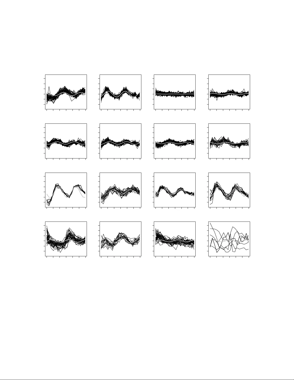
V ariational appro ximation for mixtures of linear mixed mo dels Siew Li T an and Da vid J. Nott ∗ Abstract Mixtures of linear mixed mo dels (MLMMs) are useful for clustering gr oup ed data and can b e estimated b y lik eliho o d maximization through the EM algorithm. The con ven tional approac h to determining a suitable num b er of comp onen ts is to compare differen t mixture models using p enalized log-lik eliho od criteria such as BIC. W e propose fitting MLMMs with v ariational methods which can p erform parameter estimation and mo del selection sim ultaneously . A v ariational appro ximation is describ ed where the v ariational lo wer bound and parameter up dates are in closed form, allo wing fast ev aluation. A new v ariational greedy algorithm is developed for mo del selection and learning of the mixture comp onents. This approach allo ws an automatic initialization of the algorithm and returns a plausible n um b er of mixture comp onen ts automatically . In cases of weak iden tifiability of certain mo del parameters, we use hierarc hical centering to reparametrize the mo del and show empirically that there is a gain in efficiency b y v ariational algorithms similar to that in MCMC algorithms. Related to this, we pro ve that the approximate rate of conv ergence of v ariational algorithms by Gaussian appro ximation is equal to that of the corresp onding Gibbs sampler which suggests that reparametrizations can lead to impro ved conv ergence in v ariational algorithms as well. Keywor ds : Linear mixed mo dels, Mixture mo dels, V ariational approximation, Hierarc hical cen tering. 1 In tro duction Mixtures of linear mixed models (MLMMs) are useful for clustering group ed data in applica- tions such as clustering of gene expression profiles (Celeux et al. , 2005, and Ng et al. , 2006) and electrical load series (Coke and Tsao, 2010). W e consider MLMMs where the resp onse distribution is a normal mixture with the mixture w eights v arying as a function of the co- v ariates. Our mo del includes cluster-sp ecific random effects so that observ ations from the ∗ Siew Li T an is PhD student, Department of Statistics and Applied Probabilit y , National Univ ersity of Singapore, Singap ore 117546 (email g0900760@nus.edu.sg). David J. Nott is Asso ciate Professor, De- partmen t of Statistics and Applied Probability , National Universit y of Singap ore, Singap ore 117546. (email standj@n us.edu.sg). 1 same cluster are correlated. W e prop ose fitting MLMMs with v ariational metho ds which can p erform parameter estimation and mo del selection simultaneously . Our article makes four con tributions. First, fast v ariational metho ds are developed for MLMMs and a v ariational lo wer b ound is obtained in closed form. Second, a new v ariational greedy algorithm is de- v elop ed for mo del selection and learning of the mixture comp onents. This approach handles algorithm initialization and returns a plausible n umber of mixture comp onen ts automatically . Third, we show empirically that there is a gain in efficiency by v ariational algorithms through the use of hierarchical centering reparametrization similar to that in Marko v c hain Mon te Carlo (MCMC) algorithms. F ourth, w e prov e that the approximate rate of con vergence of the v ariational algorithm by Gaussian appro ximation is equal to that of the corresp onding Gibbs sampler whic h suggests that reparametrizations can giv e improv ed conv ergence in v ariational algorithms just as in MCMC algorithms. In microarra y analysis, clustering of gene expression profiles is a v aluable exploratory to ol for the identification of p oten tially meaningful relationships b etw een genes. In the mo del- based cluster analysis con text, Luan and Li (2003) studied the clustering of genes based on time course gene expression profiles in the mixture mo del framew ork using a mixed-effects mo del with B-splines. Celeux et al. (2005) prop osed using MLMMs to accoun t for data v ariability in rep eated measuremen ts. Both of these approac hes require the indep endence assumption for genes. In contrast, Ng et al. (2006) considered MLMMs whic h allow genes within a cluster to b e correlated as the indep endence assumption may not hold for all pairs of genes (McLac hlan et al. , 2004). Booth et al. (2008) considered a multilev el linear mixed mo del (LMM) whic h includes cluster-sp ecific random effects and proposed a sto c hastic searc h algorithm for finding partitions of the data with high p osterior probability through maxi- mization of an ob jective function. F or the clustering of electrical load series, Coke and Tsao (2010) dev elop ed random effects mixture mo dels using a hierarc hical represen tation and used an an tedep endence mo del for the non-stationary random effects. MLMMs can b e estimated b y lik eliho o d maximization through the EM algorithm (Demp- ster et al. , 1977) and this metho d w as used in Luan and Li (2003), Celeux et al. (2005) and Cok e and Tsao (2010). Ng et al. (2006) dev elop ed a program called EMMIX-WIRE (EM- based MIXture analysis WIth Random Effects) for clustering correlated and replicated data. The optimal num b er of comp onents was determined by comparing differen t mixture mo dels using the BIC (Bay esian information criterion) of Sch w arz (1978) in these articles. The EM algorithm can be sensitiv e to initialization and is commonly run from multiple starting v alues to a v oid con vergence to local optima. Sc harl et al. (2010) studied the performance of different 2 initialization strategies for mixtures of regression mo dels. In the con text of Gaussian mixture mo dels, Biernac ki et al. (2003) compared simple initialization strategies and V erb eek et al. (2003) discussed a greedy approac h to the learning of Gaussian mixtures which resolv es the sensitivit y to initialization and is useful in finding the optimal num b er of components. W e prop ose fitting MLMMs with v ariational metho ds using a greedy algorithm. The MLMM w e consider is a simple generalization of that prop osed b y Ng et al. (2006) where units within eac h cluster may b e correlated. A v ariational appro ximation for this mo del is describ ed where the v ariational lo wer b ound and parameter up dates are in closed form, allo wing fast ev aluation. Ormero d and W and (2010) illustrated the use of v ariational metho ds to fit a Gaussian LMM and Armagan and Dunson (2011) used v ariational metho ds to obtain sparse appro ximate Bay es inference in the analysis of large longitudinal data sets using LMMs. Ormero d and W and (2012) recently introduced an approach called Gaussian v ariational appro ximation for fitting generalized LMMs where the distributions of random effects v ectors are approximated by Gaussian distributions. The v ariational algorithm suffers from problems of local optima and initialization strategies for the EM algorithm can often b e adapted for use with the v ariational algorithm. A common strategy is to run the v ariational algorithm starting with random initialization from multiple starting p oin ts (Bishop and Sv ens ´ en, 2003). Nott et al. (2011) used a short runs strategy similar to that recommended by Biernacki et al. (2003) where the v ariational algorithm is stopp ed prematurely and only the short run with the highest attained v alue of the v ariational low er b ound is follow ed to conv ergence. A k ey adv an tage of v ariational metho ds is the potential for simultaneous parameter es- timation and model selection and a num b er of suc h metho ds hav e b een dev elop ed for the fitting of Gaussian mixtures. Ueda and Ghahramani (2002) prop osed a v ariational Bay esian (VB) split and merge EM pro cedure to optimize an ob jective function that allows simul- taneous estimation of the parameters and the num b er of comp onents while a voiding lo cal optima. They applied this metho d to a Gaussian mixture and a mixture of exp erts regression where b oth input and output are treated as random v ariables. W u et al. (2012) developed a split and eliminate VB algorithm which attempts to split all p o orly fitted comp onents at the same time and made use of the comp onent-elimination prop ert y asso ciated with v ariational appro ximation so that no merge mo v es are required. This comp onent-elimination property w as noted previously b y A ttias (1999) and Corduneanu and Bishop (2001). McGrory and Titterington (2007) describ ed a v ariational optimization tec hnique where the algorithm is initialised with a large n umber of comp onents and mixture comp onents whose w eigh tings b ecome sufficien tly small are dropp ed out as the optimization pro ceeds. Constan tinop oulos 3 and Lik as (2007) observ ed that in this approac h, the num b er of comp onen ts in the resulting mixture can b e sensitive to the prior on the precision matrix. They proposed an incremen- tal approach where comp onen ts are added to the mixture following a splitting test where a different lo cal precision prior is sp ecified after taking in to accoun t c haracteristics of the precision matrix of the comp onent b eing tested. F or the examples in this pap er, w e hav e attempted the comp onent deletion approach of McGrory and Titterington (2007) (results not shown). W e observ ed that this metho d is more effectiv e when the num b er of comp onents required is not to o large as initializing the mixture with a large num b er of comp onents can b e computationally exp ensiv e esp ecially for large data sets. The choice of the initial num b er of mixture comp onen ts can hav e an impact on the resulting n um b er of components and it ma y not be easy to determine a suitable initial n umber. This approac h remains sensitiv e to initialization and metho ds such as running the v ariational algorithm from multiple starting p oin ts are necessary to av oid lo cal optima. W e develop a new v ariational greedy algorithm (VGA) for the learning of MLMMs. This greedy approac h is not limited to MLMMs and may be extended to fit other mo dels using v ariational metho ds. No additional deriv ations are required once the basic v ariational al- gorithm is a v ailable. Starting with one comp onent, the VGA adds new components to the mixture after searc hing for the optimal wa y to split comp onents in the curren t mixture. This approac h handles algorithm initialization automatically and returns a plausible v alue for the num b er of mixture comp onents. While this b ottom-up approac h resolv es the difficulty of estimating the upper b ound of the n umber of mixture comp onents, it can b ecome time- consuming when the num b er of comp onen ts is large, since a larger num b er of comp onents ha ve to b e tested to find the optimal wa y of splitting eac h one. Some measures are in tro- duced to k eep the search time short and the component elimination prop erty of v ariational appro ximation is used to sieve out comp onen ts which resist splitting. In situations where there is weak identification of certain mo del parameters and the v ariational algorithm conv erges very slowly , we apply hierarc hical centering (Gelfand et al. , 1995) to reparametrize the MLMM. Hierarc hical centering has been applied successfully in MCMC algorithms to obtain impro ved conv ergence (Chen et al. , 2000) and w e show empirically , that there is a similar gain in efficiency in v ariational algorithms. W e consider a case of partial cen tering, a second case of full centering and derive the corresp onding v ariational algorithms. Related to this, w e show that the appro ximate rate of con v ergence of the v ariational algorithm by Gaussian appro ximation is equal to that of the corresp onding Gibbs sampler. Sah u and Rob erts (1999) sho wed that the appro ximate rate of con v ergence of 4 the Gibbs sampler by Gaussian appro ximation is equal to that of the corresp onding EM-t yp e algorithm and hence improv emen t strategies for one algorithm can b e used for the other. As reparametrizations using hierarc hical cen tering can lead to impro v ed conv ergence in the Gibbs sampler, this result suggests that the rate of con v ergence of v ariational algorithms ma y b e impro ved through reparametrizations. Papaspiliopoulos et al. (2007) describ e cen tering and non-cen tering methodology as complemen tary tec hniques for use in parametrization of hierarc hical models to construct effectiv e MCMC algorithms. In Section 2, w e in tro duce MLMMs. Section 3 describ es fast v ariational approximation metho ds for MLMMs and Section 4 reparametrization of MLMMs through hierarc hical cen- tering. Section 5 describ es the v ariational greedy algorithm and Section 6 con tains theoretical results on the rate of conv ergence of v ariational algorithms by Gaussian approximation. Sec- tion 7 considers examples inv olving real and simulated data and Section 8 concludes. 2 Mixtures of linear mixed mo dels The MLMM w e consider is a generalization of that prop osed b y Ng et al. (2006), where units from the same cluster share cluster-sp ecific random effects and are hence correlated. Unlik e Ng et al. (2006), our mo del can fit data where the n umber of observ ations on eac h unit are not equal and we allo w the mixture w eigh ts to v ary with co v ariates b etw een clusters. Supp ose w e observe n multiv ariate rep onses y i = ( y i 1 , ..., y in i ) T , i = 1 , ..., n and N = P n i =1 n i . Let the n umber of mixture comp onents b e k and z i , i = 1 , ..., n b e latent v ariables indicating whic h mixture comp onent the i th cluster corresp onds to, z i ∈ { 1 , ..., k } . Conditional on z i = j , y i = X i β j + W i a i + V i b j +  i (1) where X i , W i and V i are design matrices of dimensions n i × p , n i × s 1 and n i × s 2 resp ectiv ely , β j , j = 1 , ..., k , are p × 1 v ectors of fixed effects, a i , i = 1 , ..., n, are s 1 × 1 vectors of random effects, b j , j = 1 , ..., k , are s 2 × 1 vectors of random effects and  i , i = 1 , ..., n, are v ectors of random errors. W e assume that the random effects a i , i = 1 , ..., n , b j , j = 1 , ..., k , and the error v ectors  i , i = 1 , ..., n, are mutually indep endent. The fixed effects, the distribution of the random effects and the distribution of the error terms are all mixture comp onen t sp ecific. The random effects distribution for a i and b j are N (0 , σ 2 a j I s 1 ) and N (0 , σ 2 b j I s 2 ) respectively . The error vector  i is distributed as N (0 , Σ ij ) where Σ ij = blo c kdiag( σ 2 j 1 I κ i 1 , ..., σ 2 j g I κ ig ), a block diagonal with the l th blo c k equal to σ 2 j l I κ il . Here g is constant for all i and P g l =1 κ il = n i for eac h i = 1 , ..., n . In microarray exp erimen ts for instance, this specification provides increased 5 flexibilit y as the error v ariance of each mixture comp onent is allow ed to v ary b etw een differen t exp erimen ts, sa y , by setting g to be the total n um b er of exp eriments. W e assume that P ( z i = j ) = p ij = exp( u T i δ j ) P l exp( u T i δ l ) (2) where u i = ( u i 1 , ..., u id ) T is a vector of co v ariates and δ j = ( δ j 1 , ..., δ j d ) T are vectors of unkno wn parameters j = 2 , ..., k . W e set δ 1 = 0 for iden tifiability . These mixing co efficien ts, whic h are functions of the cov ariates, are kno wn as gating functions in the mixture of exp erts terminology (Jacobs et al. , 1991). This mo del for the mixture comp onen t indicators allows the mixture w eights to v ary with co v ariates across clusters. F or Ba yesian inference on unknown parameters w e assume the following priors. σ 2 a j ∼ I G ( α a j , λ a j ), j = 1 , ..., k , where I G ( α, λ ) denotes the in verse gamma distribution with shap e parameter α and scale parameter λ , σ 2 b j ∼ I G ( α b j , λ b j ), j = 1 , ..., k , σ 2 j l ∼ I G ( α j l , λ j l ), j = 1 , ..., k , l = 1 , ..., g , δ = ( δ T 2 , ..., δ T k ) T ∼ N (0 , Σ δ ) and β j ∼ N (0 , Σ β j ). Here α a j , λ a j , α b j , λ b j , α j l , λ j l , Σ δ and Σ β j , j = 1 , ..., k , l = 1 , ..., g , are hyperparameters considered known. 3 V ariational appro ximation V ariational metho ds originated in statistical physics and research into these approac hes is curren tly very activ e in both statistics and machine learning. Un til recen tly , v ariational appro ximation metho ds hav e mostly b een developed in the machine learning communit y (Jordan et al. , 1999, Winn and Bishop, 2005). See Ormero d and W and (2010) for an expla- nation of v ariational appro ximation methods and the in tro duction for further references on application of v ariational metho ds to mixture mo dels sp ecifically . W e consider a v ariational appro ximation to the joint p osterior distribution of all the parameters θ of the form q ( θ | λ ) where λ is the set of v ariational parameters to b e c hosen. Here a parametric form is chosen for q ( θ | λ ) and we attempt to make q ( θ | λ ) a go o d approximation to p ( θ | y ) by minimizing the Kullbac k-Leibler (KL) divergence b etw een q ( θ | λ ) and p ( θ | y ), i.e., Z log q ( θ | λ ) p ( θ | y ) q ( θ | λ ) dθ = Z log q ( θ | λ ) p ( θ ) p ( y | θ ) q ( θ | λ ) dθ + log p ( y ) where p ( y ) = R p ( y | θ ) p ( θ ) dθ is the marginal likelihoo d. As the KL divergence is p ositiv e, log p ( y ) ≥ Z log p ( θ ) p ( y | θ ) q ( θ | λ ) q ( θ | λ ) dθ 6 whic h gives a low er bound on the log marginal lik eliho o d, and maximization of this low er b ound is equiv alent to minimisation of the KL divergence b etw een the p osterior distribution and v ariational approximation. This low er b ound is sometimes used as an approximation to the log marginal likelihoo d for Ba y esian mo del selection purp oses. W rite β = ( β T 1 , ..., β T k ) T , a = ( a T 1 , ..., a T n ) T , b = ( b T 1 , ..., b T k ) T , σ 2 a = ( σ 2 a 1 , ..., σ 2 ak ) T , σ 2 b = ( σ 2 b 1 , ..., σ 2 bk ) T , σ 2 j = ( σ 2 j 1 , ..., σ 2 j g ) T , j = 1 , ..., k , σ 2 = ( σ 2 1 T , ..., σ 2 k T ) T , δ = ( δ T 2 , ..., δ T k ) T and z = ( z 1 , ..., z n ) T so that θ = ( β T , a T , b T , σ 2 a T , σ 2 b T , σ 2 T , δ T , z T ) T . F or con venience we write q ( θ | λ ) as q ( θ ), suppressing dep endence on λ and consider a v ariational appro ximation of the form q ( θ ) = q ( β ) q ( a ) q ( b ) q ( σ 2 a ) q ( σ 2 b ) q ( σ 2 ) q ( δ ) q ( z ), where q ( β ) = k Y j =1 q ( β j ) , q ( a ) = n Y i =1 q ( a i ) , q ( b ) = k Y j =1 q ( b j ) , q ( z ) = n Y i =1 q ( z i ) , q ( σ 2 a ) = k Y j =1 q ( σ 2 a j ) , q ( σ 2 b ) = k Y j =1 q ( σ 2 b j ) , q ( σ 2 ) = k Y j =1 g Y l =1 q ( σ 2 j l ) , and q ( β j ) is N ( µ q β j , Σ q β j ), j = 1 , ..., k , q ( a i ) is N ( µ q a i , Σ q a i ), i = 1 , ..., n, q ( b j ) is N ( µ q b j , Σ q b j ), j = 1 , ..., k , q ( σ 2 a j ) is I G ( α q a j , λ q a j ), j = 1 , ..., k , q ( σ 2 b j ) is I G ( α q b j , λ q b j ), j = 1 , ..., k , q ( σ 2 j l ) is I G ( α q j l , λ q j l ), for j = 1 , ..., k , l = 1 , ..., g , q ( δ ) is a delta function placing a p oint mass of 1 on µ q δ , and q ( z i = j ) = q ij where P k j =1 q ij = 1, i = 1 , ..., n . W e are assuming in the v ariational p osterior that parameters for differen t exp ert comp onen ts are indep enden t and indep enden t of all other parameters. F or a v ariational p osterior restricted to be of the factorized form q ( θ ) = Q m i =1 q ( θ i ), the optimal q ( θ i ) minimizing the KL divergence is given by q ( θ i ) ∝ exp { E − θ i log p ( y , θ ) } (see, for example, Ormero d and W and, 2010). In our case, the sp ecific distributional forms for the v ariational p osterior densities, suc h as the assumption of a degenerate point mass v ariational p osterior for δ , hav e b een chosen to make computation of the low er b ound tractable ev en though they might not b e optimal. It is also p ossible to consider the fixed effects β , and the random effects a and b as a single blo c k and replace q ( β ) q ( a ) q ( b ) by q ( β , a, b ) as in Ormero d and W and (2010). This results in a less restricted factorization with dep endence structure b et w een β , a and b preserved and a higher low er b ound can b e ac hiev ed. Ho wev er, this will in volv e dealing with high dimensional sparse co v ariance matrices whic h creates a greater computational burden although it is p ossible to use matrix inv ersion results for the blo c k ed matrices to attain b etter computational efficiency (referee’s suggestion). W e ha ve decided to use a factorized form for faster computation and b etter scalabilit y to larger data sets 7 (see Armagan and Dunson, 2011). The indep endence and distributional assumptions made in v ariational appro ximations may not b e realistic and it has b een sho wn in the con text of Gaussian mixture mo dels that VB, which assumes a factorized p osterior, has a tendency to underestimate the p osterior v ariance (W ang and Titterington, 2005). How ever, v ariational appro ximation can often lead to go o d p oint estimates, reasonable estimates of marginal p osterior distributions and excellen t predictive inferences. Blei and Jordan (2006) show ed that predictive distributions based on v ariational appro ximations to the p osterior w ere very similar to that of MCMC for Diric hlet pro cess mixture mo dels. Braun and McAuliffe (2010) rep orted similar findings in large-scale mo dels of discrete choice although they observed that the v ariational p osterior is more concentrated around the mo de than the MCMC posterior, a familiar underdisp ersion effect noted abov e. Similar independence assumptions ha ve b een made in the case of the LMM b y Armagan and Dunson (2011). No w, we wan t to maximise the v ariational low er b ound L = R log p ( θ ) p ( y | θ ) q ( θ ) q ( θ ) dθ with resp ect to the parameters λ in our v ariational p osterior appro ximation. The low er b ound L can b e computed in closed form, and is given by (details in supplementary materials) 1 2 k X j =1 ( log | Σ − 1 β j Σ q β j | − tr(Σ − 1 β j Σ q β j ) − µ q β j T Σ − 1 β j µ q β j + log | Σ q b j | − α q b j λ q b j  µ q b j T µ q b j + tr(Σ q b j )  ) + k X j =1 ( α b j log λ b j λ q b j + log Γ( α q b j ) Γ( α b j ) − λ b j α q b j λ q b j − s 2 2 log( λ q b j ) + α q b j + α a j log λ a j λ q a j + log Γ( α q a j ) Γ( α a j ) − s 1 P n i =1 q ij 2 ( ψ ( α q a j ) − log( λ q a j )) + ψ ( α q a j )( α a j − α q a j ) − λ a j α q a j λ q a j + α q a j  + 1 2 n X i =1 log | Σ q a i | + k X j =1 g X l =1 ( α j l log λ j l λ q j l + log Γ( α q j l ) Γ( α j l ) + P n i =1 κ il q ij 2  ψ ( α q j l ) − log( λ q j l )  + ψ ( α q j l )( α j l − α q j l ) − λ j l α q j l λ q j l + α q j l ) − n X i =1 k X j =1 q ij 2  ξ T ij Σ q ij − 1 ξ ij + tr(Σ q ij − 1 Λ ij ) + α q a j λ q a j  µ q a i T µ q a i + tr(Σ q a i )   + n X i =1 k X j =1 q ij log p ij q ij + log p ( µ q δ ) + k ( p + s 2 ) + ns 1 − N log (2 π ) 2 (3) where Γ( · ) and ψ ( · ) denote the gamma and digamma functions resp ectiv ely , p ij is ev aluated b y setting δ = µ q δ , p ( µ q δ ) denotes the prior distribution for δ ev aluated at µ q δ , ξ ij = y i − X i µ q β j − W i µ q a i − V i µ q b j , Σ q ij − 1 = blo ckdiag  α q j 1 λ q j 1 I κ i 1 , ..., α q j g λ q j g I κ ig  and Λ ij = X i Σ q β j X T i + W i Σ q a i W T i + V i Σ q b j V T i . The v ariational parameters to b e optimized consist of µ q β j , Σ q β j , µ q b j , Σ q b j , α q a j , λ q a j , 8 α q b j , λ q b j , for j = 1 , ..., k , µ q a i , Σ q a i , for i = 1 , ..., n , α q j l , λ q j l , for j = 1 , ..., k , l = 1 , ..., g , q ij for i = 1 , ..., n , j = 1 , ..., k , and µ q δ . W e optimize the low er b ound with resp ect to eac h of these sets of parameters with the others held fixed in a gradien t ascen t algorithm. All up dates except for µ q δ are a v ailable in closed form and can be derived using v ector differen tial calculus (see W and, 2002). A lgorithm 1 : Initialize: q ij for i = 1 , ..., n , j = 1 , ..., k , α q j l λ q j l for j = 1 , ..., k , l = 1 , ..., g , µ q a i for i = 1 , ..., n , µ q b j , α q a j λ q a j and α q b j λ q b j for j = 1 , ..., k . Do un til the c hange in the lo wer b ound betw een iterations is less than a tolerance: 1. Σ q β j ← (Σ − 1 β j + P n i =1 q ij X T i Σ q ij − 1 X i ) − 1 . 2. µ q β j ← Σ q β j P n i =1 q ij X T i Σ q ij − 1 ( y i − W i µ q a i − V i µ q b j ) . 3. Σ q a i ←  P k j =1 q ij α q a j λ q a j I s 1 + W T i ( P k j =1 q ij Σ q ij − 1 ) W i  − 1 . 4. µ q a i ← Σ q a i P k j =1 q ij W T i Σ q ij − 1 ( y i − X i µ q β j − V i µ q b j ) . 5. Σ q b j ←  α q b j λ q b j I s 2 + P n i =1 q ij V T i Σ q ij − 1 V i  − 1 . 6. µ q b j ← Σ q b j P n i =1 q ij V T i Σ q ij − 1 ( y i − X i µ q β j − W i µ q a i ) . 7. α q a j ← α a j + s 1 2 P n i =1 q ij . 8. λ q a j ← λ a j + 1 2 P n i =1 q ij { µ q a i T µ q a i + tr(Σ q a i ) } . 9. α q b j ← α b j + s 2 2 . 10. λ q b j ← λ b j + 1 2 { µ q b j T µ q b j + tr(Σ q b j ) } . 11. α q j l ← α j l + 1 2 P n i =1 q ij κ il . 12. λ q j l ← λ j l + 1 2 P n i =1 q ij { ( ξ ij ) T κ il ( ξ ij ) κ il + tr(Λ ij ) κ il } where (( ξ ij ) κ i 1 , ..., ( ξ ij ) κ ig ) is the partition of ξ ij corresp onding to the ( κ i 1 , ..., κ ig ) and (Λ ij ) κ il is the diagonal blo ck of Λ ij with rows and columns corresponding to the position of κ il within ( κ i 1 , ..., κ ig ). 9 13. Set µ q δ to b e the conditional mode of the low er b ound fixing other v ariational parameters at their curren t v alues. As a function of µ q δ , the lo wer b ound is the log p osterior for a Ba yesian m ultinomial regression with the i th resp onse b eing ( q i 1 , ..., q ik ) T and a normal prior on µ q δ . The usual iteratively w eigh ted least squares algorithm (or other numerical optimization algorithm) can b e used for finding the mo de. 14. q ij ← p ij exp( c ij ) P k l =1 p il exp( c il ) , where c ij = s 1 2 { ψ ( α q a j ) − log ( λ q a j ) } − α q a j 2 λ q a j { µ q a i T µ q a i + tr(Σ q a i ) } + 1 2 P g l =1 κ il { ψ ( α q j l ) − log( λ q j l ) } − 1 2 { tr(Σ q ij − 1 Λ ij ) + ξ T ij Σ q ij − 1 ξ ij } . In the examples, when Algorithm 1 is used in conjunction with the V GA described in Section 5 to fit a 1-comp onent mixture, for j = 1, we set α q a j λ q a j = α q b j λ q b j = 1, α q j l λ q j l = 1 for l = 1 , ..., g , µ q b j = 0, µ q a i = 0 for i = 1 , ..., n , and q ij = 1 for i = 1 , ..., n for initialization. The v ariational p osterior for δ has b een assumed to b e a degenerate p oin t mass to mak e computation of the low er b ound tractable. Ho wev er, at conv ergence, w e relax the form of q ( δ ) to b e a normal distribution. Supp ose q ( δ ) is not sub jected to any distributional restriction, the optimal c hoice for this term is given by q ( δ ) ∝ exp ( n X i =1 k X j =1 q ij log p ij − 1 2 δ T Σ − 1 δ δ ) where p ij = exp( u T i δ j ) P l exp( u T i δ l ) . (4) If µ q δ is close to the mode, we can get a normal appro ximation to q ( δ ) by setting µ q δ as the mean and the cov ariance matrix Σ q δ as the negative inv erse Hessian of the log of (4) which is the Bay esian multinomial log p osterior considered in step 13 of Algorithm 1. W aterhouse et al. (1996) outlined a similar idea which they used at every step of their iterative algorithm. W e recommend first using a delta function approximation in the V GA and doing a one-step appro ximation after the algorithm has con verged (see Nott et al. , 2011). Using the normal appro ximation N ( µ q δ , Σ q δ ) as the v ariational p osterior for q ( δ ), the v ariational lo wer b ound is the same as in (3) except that P n i =1 P k j =1 q ij log p ij + log p ( µ q δ ) is replaced with n X i =1 k X j =1 q ij E q  log exp( u T i δ j ) P l exp( u T i δ l )  + 1 2 log | Σ − 1 δ Σ q δ | − 1 2 µ q δ T Σ − 1 δ µ q δ − 1 2 tr(Σ − 1 δ Σ q δ ) + d ( k − 1) 2 . The exp ectation of the first term, E q  log n exp( u T i δ j ) P l exp( u T i δ l ) o , is not av ailable in closed form and w e replace it with log  exp( u T i µ q δ j ) P l exp( u T i µ q δ l )  where µ q δ j is the sub vector of µ q δ corresp onding to δ j , j = 2 , ..., k , to obtain an approximation to log p ( y ). This approximation to the log marginal 10 lik eliho o d is later used in the VGA as a mo del selection criterion. 4 Hierarc hical Cen tering Gelfand et al. (1995) discussed how reparametrizations of normal LMMs using hierarc hical cen tering can impro v e con vergence in MCMC algorithms. In our later examples w e encoun ter situations where there is w eak identification of certain mo del parameters and Algorithm 1 con verges very slowly . W e apply hierarc hical cen tering and show empirically that there is a gain in efficiency in v ariational algorithms through hierarchical centering, similar to that in MCMC algorithms. In Section 6 we give some theoretical supp ort for this observ ation. W e consider a case of partially centered parametrization in which X i = W i and a second case of fully centered parametrization in which X i = W i = V i in (1). In the first case, we in tro duce η i = β j + a i conditional on z i = j so that (1) is reparametrized as y i = X i η i + V i b j +  i and η i is ‘cen tered’ ab out β j , with η i ∼ N ( β j , σ 2 a j I p ). W riting η = ( η T 1 , ..., η T n ) T , the set of unkno wn parameters is no w θ = ( β T , η T , b T , σ 2 a T , σ 2 b T , σ 2 T , δ T , z T ) T . W e replace q ( a ) in the v ariational approximation with q ( η ) = Q n i =1 q ( η i ), where q ( η i ) is N ( µ q η i , Σ q η i ), for i = 1 , ..., n . In the second case of full cen tering, w e in tro duce ρ i = ν j + a i and ν j = β j + b j , conditional on z i = j so that (1) is reparametrized as y i = X i ρ i +  i , with ρ i ‘cen tered’ ab out ν j and ν j ‘cen tered’ ab out β j . W e hav e ρ i ∼ N ( ν j , σ 2 a j I p ) and ν j ∼ N ( β j , σ 2 b j I p ). W riting ν = ( ν T 1 , ..., ν T k ) T and ρ = ( ρ T 1 , ..., ρ T n ) T , the set of unknown pa- rameters is θ = ( β T , ν T , ρ T , σ 2 a T , σ 2 b T , σ 2 T , δ T , z T ) T . W e replace q ( a ) and q ( b ) in the v ariational appro ximation with q ( ρ ) = Q n i =1 q ( ρ i ) and q ( ν ) = Q k j =1 q ( ν j ), where q ( ρ i ) is N ( µ q ρ i , Σ q ρ i ) for i = 1 , ..., n , and q ( ν j ) is N ( µ q ν j , Σ q ν j ) for j = 1 , ..., k . The v ariational algorithms with partial cen tering and full centering reparametrizations are known as ‘Algorithm 2’ and ‘Algorithm 3’ resp ectively . The v ariational lo w er b ounds and parameter up dates can b e computed as b efore and can b e found in the supplementary materials. The v ariational p osterior for δ can b e relaxed to b e a normal distribution at conv ergence and similar adjustments (discussed in Section 3) apply to the v ariational low er b ounds for Algorithms 2 and 3. 11 5 V ariational Greedy Algorithm In the greedy algorithm, V A refers to V ariational Algorithm which can b e Algorithm 1, 2 or 3. Let f k denote the k -comp onent mixture mo del and C k the set of k comp onents that form the mixture mo del f k . The greedy learning pro cedure can b e outlined as follows. 1. Compute the one-component mixture mo del f 1 using V A. 2. Find the optimal wa y to split each of the comp onents in the curren t mixture f k . This is done in the following manner. F or eac h comp onent c j ∗ ∈ C k , form A j ∗ = { i ∈ { 1 , ..., n } : j ∗ = arg max 1 ≤ j ≤ k q ij } , where { q ij , 1 ≤ i ≤ n, 1 ≤ j ≤ k } are the v ariational p osterior probabilities of f k . F or m = 1 , ..., M , • randomly partition A j ∗ in to tw o disjoint subsets A j 1 ∗ and A j 2 ∗ and form a ( k + 1)-comp onen t mixture by splitting the v ariational p osterior probabilities of c j ∗ according to A j 1 ∗ and A j 2 ∗ . That is, we create t wo sub comp onents c j 1 ∗ and c j 2 ∗ suc h that for c j l ∗ , q ij is equal to the v ariational p osterior probabilities of c j ∗ in f k if the i th observ ation lies in A j l ∗ and zero otherwise, l = 1 , 2. The v ariational parameters of c j 1 ∗ and c j 2 ∗ required for initialization of the V A are set as equal to that of c j ∗ . • V ariational parameters of all other comp onen ts are set as those in f k . In the application of th e V A, w e do not update the v ariational parameters of components in C k − c j ∗ as we are only interested in learning the optimal w a y of splitting c j ∗ . Hence, w e apply only a ‘partial’ V A during this search. F or eac h comp onen t c j ∗ ∈ C k , choose the run with the highest attained lo w er b ound among M runs as that yielding the optimal wa y of splitting c j ∗ . Let L j ∗ and f split j ∗ denote the low er b ound and ( k + 1)-comp onent mixture model respectively corresp onding to the optimal w a y of splitting c j ∗ . 3. The components in C k are sorted in descending order according to L j ∗ and then split in this order. After the l th split, the total num b er of comp onents in the mixture is k + l . Let f temp k + l denote the mixture mo del obtained after l splits. Supp ose that at the ( l + 1) th split, the comp onen t in C k b eing split is c j ∗ . W e apply a ‘partial’ V A again, k eeping fixed v ariational parameters of comp onents a waiting to b e split. F or the initialization, w e set the v ariational parameters of c j 1 ∗ and c j 2 ∗ to b e equal to those in f split j ∗ and the remaining v ariational parameters to b e equal to those in f temp k + l if l > 1 and f split j ∗ if 12 l = 1. A split is considered ‘successful’ if the estimated log marginal likelihoo d increases after the split. This pro cess of splitting comp onents is terminated once w e encounter an unsuccessful split. 4. If the total num b er of successful splits in step 3 is s , then a ( k + s )-comp onent mo del f temp k + s is obtained at the end of step 3. W e apply V A on f temp k + s un til con v ergence up dating all v ariational parameters this time to obtain mixture model f k + s . 5. Rep eat steps 2–3 until all splits of the curren t mixture mo del are unsuccessful. W e hav e exp erimented with sev eral dissimilarity measures based on Euclidean distance as w ell as v ariabilit y-weigh ted similarit y measures (Y eung et al. , 2003) in the case of rep eated data to partition A j ∗ in step 2. Generally , VGA p erformed b etter when a random partition w as used. Metho ds such as k -means clustering are also difficult to apply when there is missing data. The partitioning of A j ∗ in to t w o disjoint subsets in step 2 serv es only as an initialization to the ‘partial’ V A to b e carried out in searc h of the optimal wa y to split comp onen t c j ∗ . If we consider an outrigh t partitioning of the data by assigning observ ation i to the j ∗ th comp onen t if j ∗ = arg max 1 ≤ j ≤ k q ij where { q ij , 1 ≤ i ≤ n, 1 ≤ j ≤ k } are the v ariational p osterior probabilities, it is still possible for observ ations originally from different components to be placed in the same comp onent again in steps 3 and 4. This is due to the up dating of the v ariational p osterior probabilities q ij of all components which ha v e b een split in step 3 and that of all existing comp onen ts in step 4. The amoun t of computation is greatly reduced b y the use of a ‘partial’ V A as the algorithm con verges quickly when the v ariational parameters of all other components (except for the t wo sub comp onents arising from the comp onent b eing split) are fixed. As we are using only the run with the highest attained low er b ound out of M runs, it is not computationally efficient to contin ue ev ery run to full con v ergence and we suggest using ‘short runs’ in this searc h step. In later examples, we terminate each of these M runs once the increment in the low er b ound is less than 1. Supp ose w e are trying to split a comp onent c j ∗ in to tw o sub comp onents c j 1 ∗ and c j 2 ∗ . After applying ‘partial’ V A, the v ariational p osterior probabilities of one of the t w o sub comp onents sometimes reduce to zero for all of i = 1 , ..., n , so that the t wo sub comp onents effectiv ely reduced to one. When this happ ens on the attempt leading to the highest v ariational low er bound among all M attempts to split c j ∗ , we suggest omitting c j ∗ in future splitting tests. This reduces the num b er of comp onen ts we need to test for splitting and can b e very useful when the n um b er of comp onen ts gro ws to a large n um b er. F or the examples discussed in this pap er, we set M to b e 5 and the v ariational algorithm is deemed 13 to hav e conv erged when the absolute relative c hange in the lo w er b ound is less than 10 − 5 . W e note that the num b er of mixture comp onen ts returned by the VGA ma y v ary due to the random partitions in step 2 although the v ariation is relativel y small compared to the n umber of clusters returned. The biggest adv antage of the V GA is that it p erforms parameter estimation and mo del selection simultaneously and automatically returns a plausible n umber of comp onen ts. It is possible ho w ever for the VGA to o verestimate the n um b er of components and some optional merge mov es may b e carried out after the VGA has conv erged if the user finds certain clusters to b e very similar. This can b e done quickly using a partial ‘V A’ in whic h the v ariational parameters of all other comp onents except the t wo to b e merged are fixed. A merge mov e is considered ‘successful’ if the estimated log marginal likelihoo d increases when t wo comp onen ts are merged. While the V GA has b een applied repeatedly in the examples for the purp ose of analysing its p erformance, the user need only apply it once and may consider some merge mov es if he finds clusters which are v ery similar. If m ultiple applications are used, w e suggest using the estimated log marginal lik eliho o d as a guideline to select the clustering solution. While reparametrizations using hierarchical cen tering increases the efficiency of the V GA, we ha ve not observ ed that the num b er of comp onen ts returned differs significantly due to the reparametrization. 6 Rate of con v ergence of v ariational appro ximation In this section, w e show that the approximate rate of con v ergence of the v ariational al- gorithm by Gaussian approximation is equal to that of the corresp onding Gibbs sampler. As reparametrizations using hierarc hical cen tering can lead to impro v ed conv ergence in the Gibbs sampler, this result lends insigh t into ho w suc h reparametrizations can increase the efficiency of v ariational algorithms in the context of MLMMs. This is b ecause the joint p os- terior of the fixed and random effects in a LMM is Gaussian (with Gaussian priors and Gaussian random effects distributions) when the v ariance parameters are known. Let the complete data b e Y aug = ( Y obs , Y mis ) where Y obs is the observ ed data and Y mis is the missing data. Let the complete data lik eliho o d b e p ( Y aug | θ ) where θ is a p × 1 v ector and Y mis r × 1. Supp ose the prior for θ is p ( θ ) ∝ 1 and the target distribution is p ( θ , Y mis ) = N (( µ 1 µ 2 ) , Σ) where Σ =  Σ 11 Σ 12 Σ 21 Σ 22  . Let H = Σ − 1 =  H 11 H 12 H 21 H 22  . It can b e shown that p ( Y mis | θ , Y obs ) = N  µ 2 − H − 1 22 H 21 ( θ − µ 1 ) , H − 1 22  and p ( θ | Y mis , Y obs ) = N  µ 1 − H − 1 11 H 12 ( Y mis − µ 2 ) , H − 1 11  . 14 Sah u and Rob erts (1999) show ed that under such conditions, the rate of conv ergence of the EM algorithm alternating b etw een the t wo components θ and Y mis is equal to the rate of con vergence of the corresp onding t w o-blo c k Gibbs s ampler. This rate is given b y ρ ( B E M ), where B E M = H − 1 11 H 12 H − 1 22 H 21 and ρ ( . ) denotes the sp ectral radius of a matrix. In the v ariational approach, w e seek an approx imation q ( θ , Y mis ) to the true p osterior p ( θ , Y mis | Y obs ) for whic h the KL div ergence betw een q and p ( θ , Y mis | Y obs ) is minimized sub ject to the restriction that q ( θ , Y mis ) can b e factorized as q ( θ ) q ( Y mis ). The optimal densities are q ( Y mis ) = N  µ 2 − H − 1 22 H 21 ( µ q θ − µ 1 ) , H − 1 22  and q ( θ ) = N  µ 1 − H − 1 11 H 12 ( µ q Y mis − µ 2 ) , H − 1 11  , where µ q θ and µ q Y mis denote the mean of q ( θ ) and q ( Y mis ) resp ectively . Starting with some ini- tial estimate for µ q θ , w e can iterativ ely up date the parameters µ q θ and µ q Y mis un til conv ergence. Let µ q θ ( t ) and µ q ( t ) Y mis denote the t th iterates. It can b e sho wn that µ q ( t +1) Y mis = H − 1 22 H 21 H − 1 11 H 12 µ q ( t ) Y mis +  I r − H − 1 22 H 21 H − 1 11 H 12  µ 2 and µ q θ ( t +1) = B E M µ q θ ( t ) +  I p − B E M  µ 1 . The matrix rate of con vergence of an iterative algorithm for which θ ( t +1) = M ( θ ( t ) ) and θ ∗ is the limit is giv en by D M ( θ ∗ ) where D M ( θ ) = ( ∂ M j ( θ ) ∂ θ i ). A measure of the actual observed rate of conv ergence is giv en by the largest eigen v alue of D M ( θ ∗ ) (Meng, 1994). The rate of conv ergence of µ q θ is therefore ρ ( B E M ). Since H − 1 22 H 21 H − 1 11 H 12 and B E M share the same eigen v alues, the rate of conv ergence of µ q Y mis is also ρ ( B E M ). The o v erall rate of con vergence of the v ariational algorithm is thus ρ ( B E M ). Supp ose we imp ose a tougher restriction on q ( θ , Y mis ). F or a partition of θ into m groups suc h that θ = ( θ 1 , ..., θ m ) with θ i a r i × 1 vector and P r i = p , w e assume that q ( θ , Y mis ) can b e factorised as Q m i =1 q ( θ i ) q ( Y mis ). The optimal densit y of q ( Y mis ) remains unchanged. Let µ 1 = ( µ 11 , ..., µ 1 m ) and H 11 = Λ 11 Λ 12 ... Λ 1 m Λ 21 Λ 22 ... Λ 2 m . . . . . . . . . . . . Λ m 1 Λ m 2 ... Λ mm ! . b e partitioned according to θ = ( θ 1 , ..., θ m ). The optimal density of q ( θ i ) is N ( µ 1 i − Λ − 1 ii X j 6 = i Λ ij ( µ q θ j − µ 1 j ) − Λ − 1 ii H 12 ( µ q Y mis − µ 2 ) , Λ − 1 ii ) for i = 1 , ..., m. 15 This leads to the following iterativ e scheme. After initializing µ q θ i , i = 1 , ..., m. , we cycle though up dates: • µ q Y mis ← µ 2 − H − 1 22 H 21 ( µ q θ − µ 1 ) • µ q θ i ← µ 1 i − Λ − 1 ii P j 6 = i Λ ij ( µ q θ j − µ 1 j ) − Λ − 1 ii H 12 ( µ q Y mis − µ 2 ) , i = 1 , ..., m, till con v ergence. Consider the ( t + 1) th iteration. F or notational simplicit y , w e replace ( µ q ( t ) θ i − µ 1 i ) by λ q ( t ) θ i , ( µ q ( t ) θ − µ 1 ) by λ q ( t ) θ and ( µ q ( t ) Y mis − µ 2 ) by λ q ( t ) Y mis . Since λ q ( t +1) Y mis = − H − 1 22 H 21 λ q θ ( t ) , w e ha v e       Λ 11 0 ... 0 Λ 21 Λ 22 ... 0 . . . . . . . . . . . . Λ m 1 Λ m 2 ... Λ mm             λ q ( t +1) θ 1 λ q ( t +1) θ 2 . . . λ q ( t +1) θ m       +       0 Λ 12 ... Λ 1 m 0 0 ... Λ 2 m . . . . . . . . . . . . 0 0 ... 0             λ q ( t ) θ 1 λ q ( t ) θ 2 . . . λ q ( t ) θ m       = H 11 B E M λ q θ ( t ) . Let L b e the low er triangular matrix of H 11 and U = L − H 11 . Then Lλ q θ ( t +1) − U λ q θ ( t ) = H 11 B E M λ q θ ( t ) ⇔ λ q θ ( t +1) = L − 1 U λ q θ ( t ) + L − 1 ( L − U ) B E M λ q θ ( t ) ⇔ λ q θ ( t +1) = [ B aug + ( I p − B aug ) B E M ] λ q θ ( t ) where B aug = L − 1 U . Therefore the rate of con v ergence of λ q θ and hence, that of µ q θ is ρ ( B aug + ( I p − B aug ) B E M ). As the rate of conv ergence r , is defined as r = lim t →∞ k θ ( t +1) − θ ∗ k k θ ( t ) − θ ∗ k , the rate of con v ergence of λ q Y mis and hence µ q Y mis is giv en b y lim t →∞    λ q ( t +1) Y mis − λ q ∗ Y mis       λ q ( t ) Y mis − λ q ∗ Y mis    = lim t →∞    − H − 1 22 H 21 λ q θ ( t ) + H − 1 22 H 21 λ q θ ∗       − H − 1 22 H 21 λ q θ ( t − 1) + H − 1 22 H 21 λ q θ ∗    = lim t →∞    λ q θ ( t ) − λ q θ ∗       λ q θ ( t − 1) − λ q θ ∗    whic h is equal to the rate of con v ergence of µ q θ . The ov erall rate of conv ergence of the v aria- tional algorithm is th us ρ ( B aug + ( I p − B aug ) B E M ) whic h is equal to the rate of con vergence of the Gibbs sampler that sequentially up dates comp onents of θ , and then blo c k updates Y mis deriv ed b y Sah u and Rob erts (1999). Although the theory developed may not b e directly applicable to LMMs with unkno wn v ariance comp onents as w ell as MLMMs in general, it suggests to consider hierarc hical centering in the context of v ariational algorithms and our examples sho w that there is some gain in efficiency due to the reparametrizations. 16 7 Examples T o illustrate the metho ds prop osed, we apply V GA using Algorithms 1, 2 and 3 on three real data sets (application of Algorithm 2 on y east galactose data set can b e found in sup- plemen tary materials). W e also consider simulated data sets in Section 7.3 where V GA is compared with EMMIX-WIRE (Ng et al. , 2006). In Section 7.2, we rep ort the gain in ef- ficiency from reparametrization of the mo del using hierarchical cen tering. In the examples b elo w, an outrigh t partitioning of the data is obtained by assigning observ ation i to the j ∗ th comp onen t if j ∗ = arg max 1 ≤ j ≤ k q ij , where { q ij , 1 ≤ i ≤ n, 1 ≤ j ≤ k } are the v ariational p osterior probabilities of the mixture model obtained using V GA. 7.1 Clustering of time course data Using DNA microarrays and samples from yeast cultures synchronized b y three indep enden t metho ds, Sp ellman et al. (1998) identified 800 genes that meet an ob jectiv e minim um crite- rion for cell cycle regulation. W e consider the 18 α -factor synchronization where the y east cells were sampled at 7 min in terv als for 119 mins and a subset of 612 genes that ha v e no missing gene expression data across all 18 time points. This data set was previously analyzed b y Luan and Li (2003) and Ng et al. (2006) and is av ailable online from the yeast cell cycle analysis pro ject at h ttp://genome-www.stanford.edu/cellcycle/. Our aim is to obtain an op- timal clustering of these genes using the V GA. F ollo wing Ng et al. (2006), w e tak e n = 612 genes, W i = 1 18 , V i = I 18 , u i = 1 and X i to b e an 18 × 2 matrix with the ( l + 1)th ro w ( l = 0 , ..., 17) as (cos(2 π (7 l ) /ω ) , sin(2 π (7 l ) /ω ) , where ω = 53 is the perio d of the cell cycle for i = 1 , ..., n . F or the error terms, we take g = 1 and κ i 1 = 18 for i = 1 , ..., n so that the error v ariance of each mixture comp onen t is constant across the 18 time p oints. W e used the follo wing priors, δ ∼ N (0 , 1000 I ), β j ∼ N (0 , 1000 I ) for j = 1 , ..., k , and I G (0 . 01 , 0 . 01) for σ 2 a j , σ 2 b j , j = 1 , ..., k and σ 2 j l , j = 1 , ..., k , l = 1 , ..., g . Applying the V GA using Algorithm 1 ten times, we obtained a 15-comp onent mixture once, a 16-comp onen t mixture six times and a 17-comp onen t mixture thrice. The mo de is 16 and we rep ort the clustering for a 16-comp onent mixture obtained from the VGA in Figure 1. F or this clustering, w e attempted several merge mov es on clusters which app ear similar suc h as 3 with 4, 5 with 6, 7 with 8 and 13 with 14. These merge mo ves did not result in a higher estimated log marginal lik eliho o d. Ho wev er, w e observed that cluster 2 (48 genes) w as split into t wo clusters in one of the 17-component mixture models and these tw o clusters can b e merged successfully with a higher estimated log marginal lik eliho o d b eing obtained. 17 0 40 80 120 −2 0 2 cluster 1 (43 genes) seq(0, 119, 7) 0 40 80 120 −2 0 2 cluster 2 (48 genes) seq(0, 119, 7) comp[1, ] 0 40 80 120 −2 0 2 cluster 3 (85 genes) seq(0, 119, 7) comp[1, ] 0 40 80 120 −2 0 2 cluster 4 (49 genes) seq(0, 119, 7) comp[1, ] 0 40 80 120 −2 0 2 cluster 5 (65 genes) seq(0, 119, 7) 0 40 80 120 −2 0 2 cluster 6 (63 genes) seq(0, 119, 7) comp[1, ] 0 40 80 120 −2 0 2 cluster 7 (77 genes) seq(0, 119, 7) comp[1, ] 0 40 80 120 −2 0 2 cluster 8 (28 genes) seq(0, 119, 7) comp[1, ] 0 40 80 120 −2 0 2 cluster 9 (8 genes) seq(0, 119, 7) 0 40 80 120 −2 0 2 cluster 10 (21 genes) seq(0, 119, 7) comp[1, ] 0 40 80 120 −2 0 2 cluster 11 (18 genes) seq(0, 119, 7) comp[1, ] 0 40 80 120 −2 0 2 cluster 12 (15 genes) seq(0, 119, 7) comp[1, ] 0 40 80 120 −2 0 2 cluster 13 (34 genes) 0 40 80 120 −2 0 2 cluster 14 (16 genes) comp[1, ] 0 40 80 120 −2 0 2 cluster 15 (36 genes) comp[1, ] 0 40 80 120 −2 0 2 cluster 16 (6 genes) comp[1, ] Figure 1: Clustering results for time course data obtained from applying the V GA using Algorithm 1. The x -axis are the time p oin ts and y -axis are the gene expression lev els. Line in grey is the p osterior mean of the fixed effects giv en by X i µ q β j . 18 Cluster 1 (30) 0.5 6 12 bot 28 30 Cluster 2 (48) temp 0.5 6 12 bot 28 30 Cluster 3 (57) temp 0.5 6 12 bot 28 30 Cluster 4 (67) temp 0.5 6 12 bot 28 30 Cluster 5 (34) temp 0.5 6 12 bot 28 30 Cluster 6(54) temp 0.5 6 12 bot 28 30 Figure 2: Clustering results for w ater temp erature data. The x -axis is the depth and y -axis is the w ater temp erature. Th us, it is p ossible for the VGA to ov erestimate the num b er of mixture comp onents and merge mo ves can b e considered when similar clusters are encountered. W e note how ev er that the v ariation in the num b er of mixture comp onents returned by the VGA is relatively small. F or this data set, the num b er of clusters returned b y V GA w as generally larger than that obtained b y Ng et al. (2006) where BIC w as used for mo del selection and the optimal num b er of clusters was rep orted as 12. Any interpretation of the differences in results w ould need to b e pursued with the help of sub ject matter exp erts, but our later simulation studies tend to indicate that BIC underestimates the true mo del so that p ossibly our clustering is preferable from this point of view. Of course it ma y b e argued that the abilit y to estimate the ‘true mo del’ is not a c hief concern in clustering applications where interpretabilit y of the results in the substan tiv e scien tific con text is the primary motiv ation. 7.2 Clustering of water temp erature data W e consider the daily a verage water temp erature readings during the p erio d 9 Septem b er 2010–10 August 2011 collected at a monitoring station at Upper P eirce Reserv oir, Singap ore. No data w ere a v ailable during the p erio ds 23 Decem b er 2010–28 December 2010, 10 F ebruary 2010–23 F ebruary 2010 and 14 April 2011–10 Ma y 2011. Readings w ere collected at elev en depths from the water surface; 0.5m, 2m, 4m, 6m, 8m, 10m, 12m, 14m, 16m, 18m and at the b ottom. Using data from the remaining 290 days, we apply the VGA to obtain a clustering of this data. W e take n = 290, n i = 11 and X i = W i = V i = I 11 for i = 1 , ..., n . W e set g = 11 with κ il = 1 for i = 1 , ..., n , l = 1 , ..., g so that the error v ariance of each mixture comp onent is allow ed to be differen t at different depths. F or the mixture weigh ts, w e set u i = (1 , i, i 2 , i 3 ), i = 1 , ..., n, and subsequen tly standardize columns 2–4 in the matrix U = ( u T 1 , ..., u T n ) T to take v alues b et ween -1 and 1, centered at 0. W e used the following 19 0 150 300 0.0 0.4 0.8 Cluster 1 0 150 300 0.0 0.4 0.8 Cluster 2 0 150 300 0.0 0.4 0.8 Cluster 3 0 150 300 0.0 0.4 0.8 Cluster 4 0 150 300 0.0 0.4 0.8 Cluster 5 0 150 300 0.0 0.4 0.8 Cluster 6 Figure 3: Fitted probabilities b y gating function for clusters 1 to 6. The x -axis are days n umbered 1 to 290 and y-axis are the probabilities. priors, δ ∼ N (0 , 1000 I ), β j ∼ N (0 , 10000 I ) for j = 1 , ..., k , and I G (0 . 01 , 0 . 01) for σ 2 a j , σ 2 b j , j = 1 , ..., k and σ 2 j l , j = 1 , ..., k , l = 1 , ..., g . Applying V GA with Algorithm 3 five times, w e obtained a 6-component mo del eac h time with very similar results. The clustering of a 6-comp onen t fitted mo del is shown in Figure 2 and the fitted probabilities from the gating function are sho wn in Figure 3. F or comparison, w e apply VGA with Algorithm 1 fiv e times. A 6-comp onent mixture mo del w as obtained on all five attempts. The av erage CPU time tak en to fit a 6-comp onent mo del using V GA with Algorithm 1 was 2114 seconds compared to 932 seconds by Algorithm 3. In this example, hierarc hical centering reparametrization has help ed to improv e the rate of conv ergence with the computation time reduced b y more than half. The Upp er P eirce Reservoir uses aeration devices in tended to mix the w ater at different depths, with the aim of controlling outbreaks of ph ytoplankton and algal scums. On days when these aeration devices are operational, it is exp ected that there will b e less stratification of the temperature with depth. Accurate records of the op eration of the aeration devices were not av ailable to us and there is some interest in seeing whether the clusters divide into more or less stratified comp onents giving some insight into when the aeration devices were used. 7.3 Sim ulation study W e rep ort results from a sim ulation study in which VGA is compared with EMMIX-WIRE dev elop ed by Ng et al. (2006). EMMIX-WIRE fits MLMMs by likelihoo d maximization using the EM algorithm and is able to handle the clustering of correlated data that may b e replicated. W e compare the p erformance of EMMIX-WIRE with VGA using 10 data sets sim ulated from mo del (1). Eac h data set consist of n = 499 v ectors of dimension n i = 18 and each con tain 12 clusters of sizes 43, 48, 85, 49, 65, 77, 8, 21, 18, 15, 34 and 36. These clusters are based on the 16-comp onent mixture mo del in Figure 1 fitted to the time course 20 EMMIX-WIRE V GA Optimal 17-comp Optimal Data No. of clusters mo del mo del No. of clusters mo del set in optimal mo del ARI ARI in optimal mo del ARI 1 8 0.658 0.725 12 0.966 2 8 0.606 0.837 12 0.898 3 8 0.534 0.724 11 0.774 4 9 0.774 0.808 13 0.928 5 8 0.604 0.724 12 0.951 6 7 0.545 0.904 12 0.951 7 7 0.500 0.697 11 0.779 8 8 0.649 0.642 12 0.888 9 6 0.522 0.537 11 0.755 10 6 0.485 0.684 12 0.922 T able 1: Sim ulation results comparing EMMIX-WIRE with VGA. data in Section 7.1 from whic h 12 distinctive clusters hav e b een selected. In particular, w e ha ve left out clusters 6, 8, 14 and 16. The v alues of the unknown parameters β j , σ 2 a j , σ 2 b j , j = 1 , ..., k , and σ 2 j l , j = 1 , ..., k , l = 1 , ..., g in mo del (1) were tak en to b e equal to the v ariational p osterior mean v alues of the 16-comp onent mixture in Figure 1 and g = 1. The design matrices X i , W i and V i , i = 1 , ..., n, are as describ ed in Section 7.1 and we used the same priors as b efore. F or eac h of the 10 data sets, we ran EMMIX-WIRE with the num b er of comp onents rang- ing from 6 to 15 and used the BIC for mo del selection. The optimal n um b er of components is tak en to b e that whic h minimizes − 2 log( Lik ) + ( par ) log n, where par denotes the n um b er of parameters in the model and Lik is the likelihoo d. W e used the appro ximation of Lik from the output of EMMIX-WIRE for the computation of the BIC. See Ng et al. (2006) for details on how the likelihoo d w as appro ximated. W e ran EMMIX-WIRE again, this time fixing the n umber of components as 12. W e also applied the V GA with Algorithm 1 once for eac h of the 10 data sets. The adjusted Rand Index (ARI) (Hubert and Arabie, 1985) for the clustering of the fitted model relative to the true grouping of all 499 observ ations into 12 clusters was then computed in eac h case. The results are summarized in T able 1. F rom T able 1, the ARI attained by V GA was consisten tly higher than that attained by EMMIX-WIRE. It is also in teresting to note that in almost all the ten sets of simulated data, the ARI attained by the 12-comp onen t mo del fitted b y EMMIX-WIRE w as higher than that attained by the optimal mo del iden tified by BIC. So BIC tends to underestimate the n umber of comp onents here, although the implications of this for applications in clustering algorithms may b e less clear. 21 8 Conclusion W e hav e prop osed fitting MLMMs with v ariational metho ds and developed an efficient V GA whic h is able to p erform parameter estimation and mo del selection sim ultaneously . This greedy approach handles initialization automatically and returns a plausible v alue for the n umber of mixture comp onen ts. The exp eriments we ha v e conducted sho wed that the VGA do es not systematically underestimate nor ov erestimate the n um b er of mixture comp onen ts. F or the simulated data sets considered, V GA w as able to return mixture mo dels where the n umber of mixture comp onents is very close to the correct n um b er of comp onen ts. W e further sho wed empirically that hierarc hical cen tering can help to improv e the rate of con vergence in v ariational algorithms significan tly . Some theoretical supp ort was also pro vided for this ob- serv ation. Implemen tation of the VGA is straightforw ard as no further deriv ation is required once the basic v ariational algorithms are a v ailable. This greedy approach is not limited to MLMMs and could p otentially b e extended to fitting other mo dels using v ariational meth- o ds. All co de w as written in the R language and run on a dual pro cessor Window PC 3GHz w orkstation. 9 Supplemen tary materials The deriv ation of the v ariational lo w er bound in (3) and the expressions of the v ariational lo wer b ounds and parameter up dates for Algorithms 2 and 3 can b e found in the supple- men tary materials. An example on application of Algorithm 2 to yeast galactose data is also included. 10 Ac kno wledgemen ts Siew Li T an w as partially supp orted as part of the Singap ore-Delft W ater Alliance (SDW A)’s tropical reservoir researc h programme. W e thank SD W A for supplying the w ater temp erature data set and Dr Da vid Burger and Dr Hans Los for their v aluable commen ts and suggestions. References Armagan, A. and Dunson, D. (2011). Sparse v ariational analysis of linear mixed models for large data sets. Statistics and Pr ob ability L etters , 81, 1056–1062. 22 A ttias, H. (1999). Inferring parameters and structure of laten t v ariable models b y v ariational Ba y es. In Pr o c e e dings of the 15th Confer enc e on Unc ertainty in A rtificial Intel ligenc e , 21–30. Blei, D.M. and Jordan, M.I. (2006). V ariational inference for Dirichlet pro cess mixtures. Bayesian A nalysis , 1, 121–144. Braun, M. and McAuliffe, J. (2010). V ariational inference for large-scale mo dels of discrete choice. Journal of the Americ an Statistic al Asso ciation , 105, 324–335. Biernac ki, C., Celeux, G. and Gov aert, G. (2003). Cho osing starting v alues for the EM algorithm for getting the highest lik eliho o d in m ultiv ariate Gaussian mixture mo dels. Computational Statistics and Data Analysis , 41, 561–575. Bishop, C.M. and Svens ´ en, M. (2003). Bay esian hierarchical mixtures of exp erts. In Pr o c e e dings of the 19th Confer enc e on Unc ertainty in Artificial Intel ligenc e , 57–64. Bo oth, J.G., Casella, G. and Hobert, J.P . (2008). Clustering using ob jective functions and sto c hastic searc h. Journal of the R oyal Statistic al So ciety: Series B , 70, 119–139. Celeux, G., Martin O. and La vergne C. (2005). Mixture of linear mixed mo dels for clustering gene expression profiles from rep eated microarray exp eriments. Statistic al Mo del ling , 5, 243–267. Chen, M.H., Shao, Q.M. and Ibrahim, J.G. (2000). Monte Carlo metho ds in Bayesian c omputation . Springer. Cok e, G. and Tsao, M. (2010). Random effects mixture mo dels for clustering electrical load series. Journal of Time Series Analysis , 31, 451–464. Constan tinop oulos, C. and Lik as, A. (2007). Unsup ervised learning of Gaussian mixtures based on v ariational comp onen t splitting. IEEE T r ansactions on Neur al Networks , 18, 745–755. Cordunean u, A, and Bishop, C.M. (2001). V ariational Ba y esian mo del selection for mixture distri- butions. In Pr o c e e dings of 8th International Confer enc e on Artificial Intel ligenc e and Statistics , 27–34. Dempster, A.P ., Laird, N.M. and Rubin, D.B. (1977). Maxim um lik eliho o d from incomplete data via the EM algorithm. Journal of the R oyal Statistic al So ciety: Series B , 39, 1–38. Gelfand, A.E., Sah u, S.K. and Carlin, B.P . (1995). Efficien t parametrisations for normal linear mixed mo dels. Biometrika , 82, 479–488. 23 Hub ert, L. and Arabie, P . (1985). Comparing partitions. Journal of Classific ation , 2, 193–218. Jacobs, R.A., Jordan, M.I., Nowlan, S.J. and Hinton, G.E. (1991). Adaptiv e mixtures of lo cal exp erts. Neur al Computation , 3, 79–87. Jordan, M.I., Ghahramani, Z., Jaakkola, T.S., Saul, L.K. (1999). An introduction to v ariational metho ds for graphical mo dels. Machine L e arning , 37, 183–233. Luan, Y. and Li, H. (2003). Clustering of time-course gene expression data using a mixed-effects mo del with B-splines. Bioinformatics , 19, 474–482. McGrory , C.A. and Titterington, D.M. (2007). V ariational appro ximations in Ba yesian mo del selec- tion for finite mixture distributions. Computational Statistics and Data Analysis , 51, 5352–5367. McLac hlan, G.J., Do, K.A. and Ambroise, C. (2004). A nalyzing micr o arr ay gene expr ession data . New Y ork: Wiley . Meng, X.L. (1994). On the rate of con v ergence of the ECM algorithm. A nnals of Statistics , 22, 326–339. Ng, S.K., McLac hlan, G.J., W ang, K., Ben-T ovim Jones, L. and Ng, S.-W. (2006). A mixture mo del with random-effects comp onen ts for clustering correlated gene-expression profiles. Bioinformat- ics , 22, 1745–1752. Nott, D.J., T an, S.L., Villani, M. and Kohn, R. (2011). Regression density estimation with v aria- tional metho ds and sto chastic approximation. Journal of Computational and Gr aphic al Statis- tics , to app ear. Preprint: h ttp://www.mattiasvillani.com/wp-conten t/uploads/2011/07/v aria tional-heteroscedastic-mo e-july-6-20114.p df Ormero d, J.T. and W and, M.P . (2010). Explaining v ariational appro ximations. The Americ an Statistician , 64, 140–153. Ormero d, J.T. and W and, M.P . (2012). Gaussian v ariational appro ximate inference for generalized linear mixed mo dels. Journal of Computational and Gr aphic al Statistics , 21, 2–17. P apaspiliop oulos, O., Rob erts, G.O. and Sk¨ old, M. A general framework for the parametrization of hierarc hical mo dels. Statistic al Scienc e , 22, 59–73. Sah u, S.K. and Rob erts, G.O. (1999). On con vergence of the EM algorithm and the Gibbs sampler. Statistics and Computing , 9, 55–64. 24 Sc harl, T., Gr ¨ un, B. and Leisch, F. (2010). Mixtures of regression mo dels for time course gene expression data: ev aluation of initialization and random effects. Bioinformatics , 26, 370–377. Sc hw arz, G. (1978). Estimating the dimension of a mo del. Annals of Statistics , 6, 461–464. Sp ellman, P .T., Sherlo ck, G., Zhang, M.Q., Iyer, V.R., Anders, K., Eisen, M.B., Bro wn, P .O., Botstein, D. and F utcher, B. (1998). Comprehensive identification of cell cycle-regulated genes of the y east Sacc haromyces cerevisiae b y microarra y h ybridization. Mole cular Biolo gy of the Cel l , 9, 3273–3297. Ueda, N. and Ghahramani, Z. (2002). Ba yesian mo del searc h for mixture mo dels based on optimiz- ing v ariational b ounds. Neur al Networks , 15, 1223–1241. V erb eek, J.J., Vlassis, N. and Kr¨ ose, B. (2003). Efficient greedy learning of Gaussian mixture mo dels. Neur al Computation , 15, 469–485. W and, M.P . (2002). V ector differential calculus in statistics. The Americ an Statistician , 56, 55–62. W ang, B. and Titterington, D.M. (2005). Inadequacy of in terv al estimates corresp onding to v aria- tional Bay esian approximations. In Pr o c e e dings of the 10th International Workshop on A rtificial Intel ligenc e , 373–380. W aterhouse, S., MacKay , D. and Robinson, T. (1996). Bay esian metho ds for mixtures of exp erts. A dvanc es in Neur al Information Pr o c essing Systems 8 , 351–357. Winn, J. and Bishop, C.M. (2005). V ariational message passing. Journal of Machine L e arning R ese ar ch , 6, 661–694. W u, B., McGrory , C.A. and P ettitt, A.N. (2012). A new v ariational Ba yesian algorithm with ap- plication to human mobilit y pattern mo deling. Statistics and Computing , 22, 185–203. Y eung, K.Y., Medvedo vic, M. and Bumgarner, R.E. (2003). Clustering gene-expression data with rep eated measurements. Genome Biolo gy , 4, Article R34. 25 Supplemen tary materials for “V ariational appro ximation for mixtures of linear mixed mo dels” Siew Li T an and Da vid J. Nott Deriv ation of v ariational lo w er b ound The v ariational lo w er b ound can b e written as E q (log p ( y , θ )) − E q (log q ( θ )), where E q ( · ) denotes the exp ectation with resp ect to q . Consider the first term, E q (log p ( y , θ )). Let ζ ij = I ( z i = j ) where I ( · ) denotes the indicator function. W e ha v e log p ( y , θ ) = n X i =1 k X j =1 ζ ij n log p ( y i | z i = j, β j , a i , b j , Σ ij ) + log p ( a i | σ 2 a j ) + log p ij o + log p ( δ ) + k X j =1 ( log p ( β j ) + log p ( b j | σ 2 b j ) + log p ( σ 2 a j ) + log p ( σ 2 b j ) + g X l =1 log p ( σ 2 j l ) ) . T aking exp ectations with resp ect to q , we obtain E q (log p ( y , θ )) = n X i =1 k X j =1 q ij ( − g X l =1 κ il 2 (log( λ q j l ) − ψ ( α q j l )) − 1 2 ( ξ T ij Σ q ij − 1 ξ ij + tr(Σ q ij − 1 Λ ij )) − s 1 2 (log λ q a j − ψ ( α q a j )) − α q a j 2 λ q a j  tr(Σ q a i ) + µ q a i T µ q a i  + log p ij  + log p ( µ q δ ) − 1 2 k X j =1 n log | Σ β j | + tr(Σ − 1 β j Σ q β j ) + µ q β j T Σ − 1 β j µ q β j + s 2 (log λ q b j − ψ ( α q b j )) + α q b j λ q b j (tr(Σ q b j ) + µ q b j T µ q b j ) ) + k X j =1  α a j log λ a j − log Γ( α a j ) − λ a j α q a j λ q a j − ( α a j + 1)(log λ q a j − ψ ( α q a j )) + α b j log λ b j − log Γ( α b j ) − λ b j α q b j λ q b j − ( α b j + 1)(log λ q b j − ψ ( α q b j )) + g X l =1 " α j l log λ j l − log Γ( α j l ) − λ j l α q j l λ q j l − ( α j l + 1)  log λ q j l − ψ ( α q j l )  − N + k ( p + s 2 ) + ns 1 2 log(2 π ) , (1) 1 where Γ( · ) and ψ ( · ) denote the gamma and digamma functions resp ectiv ely , p ij is ev aluated b y setting δ = µ q δ , p ( µ q δ ) denotes the prior distribution for δ ev aluated at µ q δ , ξ ij = y i − X i µ q β j − W i µ q a i − V i µ q b j , Σ q ij − 1 = blo ckdiag  α q j 1 λ q j 1 I κ i 1 , ..., α q j g λ q j g I κ ig  and Λ ij = X i Σ q β j X T i + W i Σ q a i W T i + V i Σ q b j V T i . T urning to the second term, E q (log q ( θ )), we hav e E q (log q ( θ )) = k X j =1 E q ( log q ( β j ) + log q ( b j ) + log q ( σ 2 b j ) + log q ( σ 2 a j ) + g X l =1 log q ( σ 2 j l ) ) + n X i =1 E q (log q ( a i )) + n X i =1 k X j =1 q ij log q ij = k X j =1  − 1 2 (log | Σ q β j | + log | Σ q b j | ) + α q b j log λ q b j − ( α q b j + 1)(log λ q b j − ψ ( α q b j )) − log Γ( α q b j ) − α q b j + α q a j log λ q a j − ( α q a j + 1)(log λ q a j − ψ ( α q a j )) − log Γ( α q a j ) − α q a j + g X l =1  α q j l log λ q j l − log Γ( α q j l ) − α q j l − ( α q j l + 1)  log λ q j l − ψ ( α q j l )  ) − 1 2 n X i =1 log | Σ q a i | − k ( p + s 2 ) + ns 1 2 (log(2 π ) + 1) + n X i =1 k X j =1 q ij log q ij (2) and putting (1) and (2) together gives the low er b ound. Algorithm 2 (partial cen tering when X i = W i ) (Up dates in steps 5, 7, 9, 10, 11 and 13 remain the same as in Algorithm 1 with s 1 = p .) Initialize: q ij for i = 1 , ..., n , j = 1 , ..., k , µ q b j , µ q β j , α q a j λ q a j and α q b j λ q b j for j = 1 , ..., k , α q j l λ q j l for j = 1 , ..., k , l = 1 , ..., g . Do until the change in the lo wer b ound b etw een iterations is less than a tolerance: 1. Σ q η i ←  P k j =1 q ij α q a j λ q a j I p + X T i ( P k j =1 q ij Σ q ij − 1 ) X i  − 1 . 2. µ q η i ← Σ q η i P k j =1 q ij n α q a j λ q a j µ q β j + X T i Σ q ij − 1 ( y i − V i µ q b j ) o 3. Σ q β j ←  Σ − 1 β j + α q a j λ q a j P n i =1 q ij I p  − 1 . 4. µ q β j ← Σ q β j α q a j λ q a j P n i =1 q ij µ q η i . 2 6. µ q b j ← Σ q b j P n i =1 q ij V T i Σ q ij − 1  y i − X i µ q η i  . 8. λ q a j ← λ a j + 1 2 P n i =1 q ij { ( µ q η i − µ q β j ) T ( µ q η i − µ q β j ) + tr(Σ q η i + Σ q β j ) } . 12. λ q j l ← λ j l + 1 2 P n i =1 q ij n ( ω ij ) T κ il ( ω ij ) κ il + tr( X i Σ q η i X T i + V i Σ q b j V T i ) κ il o , where ω ij = y i − X i µ q η i − V i µ q b j . 14. q ij ← p ij exp( c ij ) P k l =1 p il exp( c il ) , where c ij = p 2 ( ψ ( α q a j ) − log λ q a j ) − 1 2 n ω T ij Σ q ij − 1 ω ij + tr(Σ q ij − 1 ( X i Σ q β j X T i + V i Σ q b j V T i )) o + g X l =1 κ il 2 ( ψ ( α q j l ) − log λ q j l ) − α q a j 2 λ q a j n ( µ q η i − µ q β j ) T ( µ q η i − µ q β j ) + tr(Σ q η i + Σ q β j ) o The v ariational low er b ound is given by 1 2 k X j =1 ( log | Σ − 1 β j Σ q β j | − tr(Σ − 1 β j Σ q β j ) − µ q β j T Σ − 1 β j µ q β j + log | Σ q b j | − α q b j λ q b j  µ q b j T µ q b j + tr(Σ q b j )  ) + k X j =1 ( α a j log λ a j λ q a j + log Γ( α q a j ) Γ( α a j ) + p 2 n X i =1 q ij ( ψ ( α q a j ) − log λ q a j ) + ψ ( α q a j )( α a j − α q a j ) + α q a j − λ a j α q a j λ q a j + α b j log λ b j λ q b j + log Γ( α q b j ) Γ( α b j ) − λ b j α q b j λ q b j − s 2 2 log λ q b j + α q b j + g X l =1 " α j l log λ j l λ q j l + α q j l + log Γ( α q j l ) Γ( α j l ) − n X i =1 κ il q ij 2  ψ ( α q j l ) − log λ q j l  + ψ ( α q j l )( α j l − α q j l ) − λ j l α q j l λ q j l #) − N 2 log(2 π ) − n X i =1 k X j =1 q ij 2  ω T ij Σ q ij − 1 ω ij + tr(Σ q ij − 1 ( X i Σ q η i X T i + V i Σ q b j V T i )) − α q a j λ q a j  tr(Σ q η i + Σ q β j )+ ( µ q η i − µ q β j ) T ( µ q η i − µ q β j )  − 2 log p ij q ij  + k ( p + s 2 ) + np 2 + 1 2 n X i =1 log | Σ q η i | + log p ( µ q δ ) where ω ij = y i − X i µ q η i − V i µ q b j . In the examples, when Algorithm 2 is used in conjunction with the VGA to fit a 1-component mixture ( j = 1), w e set q ij = 1 for i = 1 , ..., n , α q j l λ q j l = 1 for l = 1 , ..., g , α q b j λ q b j = 1, α q a j λ q a j = 0 . 1, µ q b j = 0 and µ q β j = 0 for initialization . 3 Algorithm 3 (full cen tering when X i = W i = V i ) (Up dates in steps 7, 9, 11 and 13 remain the same as in algorithm 1 with s 1 = s 2 = p .) Initialize: q ij for i = 1 , ..., n , j = 1 , ..., k , µ q ν j , µ q β j α q a j λ q a j and α q b j λ q b j for j = 1 , ..., k , α q j l λ q j l for j = 1 , ..., k , l = 1 , ..., g . Do until the c hange in the lo wer b ound b et ween iterations is less than a tolerance: 1. Σ q ρ i ←  P k j =1 q ij α q a j λ q a j I p + X T i ( P k j =1 q ij Σ q ij − 1 ) X i  − 1 . 2. µ q ρ i ← Σ q ρ i P k j =1 q ij  α q a j λ q a j µ q ν j + X T i Σ q ij − 1 y i  . 3. Σ q ν j ←  α q b j λ q b j + α q a j λ q a j P n i =1 q ij  I p  − 1 . 4. µ q ν j ← Σ q ν j  α q b j λ q b j µ q β j + α q a j λ q a j P n i =1 q ij µ q ρ i  . 5. Σ q β j ←  Σ − 1 β j + α q b j λ q b j I p  − 1 . 6. µ q β j ← Σ q β j α q b j λ q b j µ q ν j . 8. λ q a j ← λ a j + 1 2 P n i =1 q ij { ( µ q ρ i − µ q ν j ) T ( µ q ρ i − µ q ν j ) + tr(Σ q ρ i + Σ q ν j ) } . 10. λ q b j ← λ b j + 1 2 { ( µ q ν j − µ q β j ) T ( µ q ν j − µ q β j ) + tr(Σ q ν j + Σ q β j ) } . 12. λ q j l ← λ j l + 1 2 P n i =1 q ij  ( y i − X i µ q ρ i ) T κ il ( y i − X i µ q ρ i ) κ il + tr( X i Σ q ρ i X T i ) κ il  . 14. q ij ← p ij exp( c ij ) P k l =1 p il exp( c il ) , where c ij = p 2  ψ ( α q a j ) − log λ q a j  − 1 2  ( y i − X i µ q ρ i ) T Σ q ij − 1 ( y i − X i µ q ρ i ) + tr(Σ q ij − 1 X i Σ q ρ i X T i )  − α q a j 2 λ q a j  ( µ q ρ i − µ q ν j ) T ( µ q ρ i − µ q ν j ) + tr(Σ q ρ i + Σ q ν j )  + g X l =1 κ il 2  ψ ( α q j l ) − log λ q j l  . 4 The v ariational low er b ound is given by − 1 2 k X j =1 n log | Σ − 1 β j Σ q β j | + tr(Σ − 1 β j Σ q β j ) + µ q β j T Σ − 1 β j µ q β j − log | Σ q ν j | o + 1 2 n X i =1 log | Σ q ρ i | + k X j =1 ( α a j log λ a j λ q a j + log Γ( α q a j ) Γ( α a j ) + α q a j + p 2 n X i =1 q ij ( ψ ( α q a j ) − log λ q a j ) + ψ ( α q a j )( α a j − α q a j ) − λ a j α q a j λ q a j + α b j log λ b j λ q b j + log Γ( α q b j ) Γ( α b j ) − λ b j α q b j λ q b j − p 2 log λ q b j + α q b j ) + k X j =1 g X l =1 ( α j l log λ j l λ q j l + ψ ( α q j l )( α j l − α q j l ) + log Γ( α q j l ) Γ( α j l ) + n X i =1 κ il q ij 2  ψ ( α q j l ) − log λ q j l  − λ j l α q j l λ q j l + α q j l ) − k X j =1 α q b j 2 λ q b j  ( µ q ν j − µ q β j ) T ( µ q ν j − µ q β j ) + tr(Σ q ν j + Σ q β j )  + n X i =1 k X j =1 q ij log p ij q ij + p (2 k + n ) 2 − n X i =1 k X j =1 q ij 2 n ( y i − X i µ q ρ i ) T Σ q ij − 1 ( y i − X i µ q ρ i ) + tr(Σ q ij − 1 ( X i Σ q ρ i X T i )) o + log p ( µ q δ ) − n X i =1 k X j =1 q ij α q a j 2 λ q a j  tr(Σ q ρ i + Σ q ν j ) + ( µ q ρ i − µ q ν j ) T ( µ q ρ i − µ q ν j )  − N 2 log(2 π ) . In the examples, when Algorithm 3 is used in conjunction with the VGA to fit a 1-component mixture ( j = 1), w e set q ij = 1 for i = 1 , ..., n , α q j l λ q j l = 10 for l = 1 , ..., g , α q a j λ q a j = 0 . 1, α q b j λ q b j = 0 . 01, µ q β j = 0 and µ q ν j = 0 for initialization. W e note that the rate of conv ergence of Algorithm 3 can b e sensitive to the initialization of α q j l λ q j l , α q a j λ q a j and α q b j λ q b j and observ ed that an initialization satisfying α q b j λ q b j < α q a j λ q a j < α q j l λ q j l w orks better. Example on clustering of y east galactose data The yeast galactose data of Idek er et al. (2001) has four replicate hybridizations for each of 20 cDNA arra y exp eriments. W e consider a subset of 205 genes previously analyzed b y Y eung et al. (2003) and Ng et al. (2006) whose expression patterns reflect four functional categories in the Gene Ontology (GO) listings (Ash burner et al. , 2000). This dataset is av ailable from the online v ersion of Y eung et al. (2003). Appro ximately 8% of the data are missing and Y eung et al. (2003) used a k -nearest neighbour metho d to impute the missing data v alues. Y eung et al. (2003) and Ng et al. (2006) ev aluated the p erformance of their clustering algorithms b y 5 ho w closely the clusters compared with the four categories in the GO listings. They used the adjusted Rand index (Hub ert and Arabie, 1985) to assess the degree of agreement b et ween their partitions and the four functional categories. W e use this example to illustrate the wa y that our mo del can mak e use of co v ariates in the mixing w eights, unlike previous analyses of this data set. In particular, we use the GO listings as cov ariates in the mixture w eigh ts. Let u i b e a vector of length d = 4 where the l th elemen t is 1 if the functional category of gene i is l and 0 otherwise. Instead of lo oking at the data with the missing v alues imputed by the k -nearest neigh b our metho d, we consider the original data containing 8% missing v alues, since our mo del has the capability to handle missing data. T aking n = 205 genes, let y itr denote the r th repetition of the expression profile for gene i at exp eriment t , 0 ≤ r ≤ 4, and R it denote the num b er of replicate hybridizations data a v ailable for gene i in exp eriment t , i = 1 , ..., 205, t = 1 , ..., 20. F or eac h i = 1 , ..., n , y i is a v ector of n i observ ations where n i = P 20 t =1 R it and y i = ( y i 11 , ..., y i 14 , ..., y i, 20 , 1 , ..., y i, 20 , 4 ) T , with missing observ ations omitted. V i is a n i × 80 matrix obtained from I 80 b y removing the ( tr )th ro w if the observ ation for experiment t at the r th rep etition is not av ailable. X i is a n i × 20 matrix, X i =       1 R i 1 0 R i 1 ... 0 R i 1 0 R i 2 1 R i 2 ... 0 R i 2 . . . . . . . . . . . . 0 R i 20 0 R i 20 ... 1 R i 20       , and W i = X i . F or the error terms, we set g = 20 with κ il = R il , i = 1 , ..., n , l = 1 , ..., g , so that the error v ariance of each mixture comp onent is allo wed to v ary b etw een different exp erimen ts. W e used the following priors, δ ∼ N (0 , 1000 I ), β j ∼ N (0 , 1000 I ) for j = 1 , ..., k , and I G (0 . 01 , 0 . 01) for σ 2 a j , σ 2 b j , j = 1 , ..., k and σ 2 j l , j = 1 , ..., k , l = 1 , ..., g . Applying the VGA using Algorithm 2 fiv e times, w e obtained a 8-comp onen t mixture on all fiv e trials with similar results. The clustering of a 8-comp onen t mixture with the highest estimated log marginal lik eliho o d among the five trials is sho wn in Figure 1. Our clustering results are slightly differen t from Ng et al (2006) where the n umber of optimal clusters obtained was 7. W e note that genes from Category 1 were split in to 3 clusters by the V GA on all 5 attempts while in Ng et al (2006), genes from Category 1 w ere sub divided into 2 clusters. In addition, instead of having one cluster containing all the genes from Category 4, we observ ed that t wo or three of the genes in Category 4 were consisten tly separated from the cluster con taining the remaining genes from Category 4. Fitted probabilities from the gating function are sho wn in Figure 2. These w ere obtained b y substituting δ with µ q δ from 6 ● ● ● ● ● ● ● ● ● ● ● ● ● ● ● ● ● ● 5 10 15 20 −2 −1 0 1 2 cluster 5 (37 genes) ● ● ● ● ● ● ● ● ● ● ● ● ● ● ● ● ● ● ● ● ● ● ● ● ● ● ● ● ● ● ● ● ● ● ● ● ● ● ● ● ● ● ● ● ● ● ● ● ● ● ● ● ● ● ● ● ● ● ● ● ● ● ● ● ● ● ● ● ● ● ● ● ● ● ● ● ● ● ● ● ● ● ● ● ● ● ● ● ● ● ● ● ● ● ● ● ● ● ● ● ● ● ● ● ● ● ● ● ● ● ● ● ● ● ● ● ● ● ● ● ● ● ● ● ● ● ● ● ● ● ● ● ● ● ● ● ● ● ● ● ● ● ● ● ● ● ● ● ● ● ● ● ● ● ● ● ● ● ● ● ● ● ● ● ● ● ● ● ● ● ● ● ● ● ● ● ● ● ● ● ● ● ● ● ● ● ● ● ● ● ● ● ● ● ● ● ● ● ● ● ● ● ● ● ● ● ● ● ● ● ● ● ● ● ● ● ● ● ● ● ● ● ● ● ● ● ● ● ● ● ● ● ● ● ● ● ● ● ● ● ● ● ● ● ● ● ● ● ● ● ● ● ● ● ● ● ● ● ● ● ● ● ● ● ● ● ● ● ● ● ● ● ● ● ● ● ● ● ● ● ● ● ● ● ● ● ● ● ● ● ● ● ● ● ● ● ● ● ● ● ● ● ● ● ● ● ● ● ● ● ● ● ● ● ● ● ● ● ● ● ● ● ● ● ● ● ● ● ● ● ● ● ● ● ● ● ● ● ● ● ● ● ● ● ● ● ● ● ● ● ● ● ● ● ● ● ● ● ● ● ● ● ● ● ● ● ● ● ● ● ● ● ● ● ● ● ● ● ● ● ● ● ● ● ● ● ● ● ● ● ● ● ● ● ● ● ● ● ● ● ● ● ● ● ● ● ● ● ● ● ● ● ● ● ● ● ● ● ● ● ● ● ● ● ● ● ● ● ● ● ● ● ● ● ● ● ● ● ● ● ● ● ● ● ● ● ● ● ● ● ● ● ● ● ● ● ● ● ● ● ● ● ● ● ● ● ● ● ● ● ● ● ● ● ● ● ● ● ● ● ● ● ● ● ● ● ● ● ● ● ● ● ● ● ● ● ● ● ● ● ● ● ● ● ● ● ● ● ● ● ● ● ● ● ● ● ● ● ● ● ● ● ● ● ● ● ● ● ● ● ● ● ● ● ● ● ● ● ● ● ● ● ● ● ● ● ● ● ● ● ● ● ● ● ● ● ● ● ● ● ● ● ● ● ● ● ● ● ● ● ● ● ● ● ● ● ● ● ● ● ● ● ● ● ● ● ● ● ● ● ● ● ● ● ● ● ● ● ● ● ● ● ● ● ● ● ● ● ● ● ● ● ● ● ● ● ● ● ● ● ● ● ● ● ● ● ● ● ● ● ● ● ● ● ● ● ● ● ● ● ● ● ● ● ● ● ● ● ● ● ● ● ● ● ● ● ● ● ● ● ● ● ● ● ● ● ● ● ● ● ● ● ● ● ● ● ● ● ● ● ● ● ● ● ● ● ● ● ● ● ● ● ● ● ● ● ● ● ● ● ● ● ● ● ● ● ● ● ● ● ● ● ● ● ● ● ● ● ● ● ● ● ● ● ● ● ● ● ● ● ● ● ● ● ● ● ● ● ● ● ● ● ● ● ● ● ● ● ● ● ● ● ● ● ● ● ● ● ● ● ● ● ● ● ● ● ● ● ● ● ● ● ● ● ● ● ● ● ● ● ● ● ● ● ● ● ● ● ● ● ● ● ● ● ● ● ● ● ● ● ● ● ● ● ● ● ● ● ● ● ● ● ● ● ● ● ● ● ● ● ● ● ● ● ● ● ● ● ● ● ● ● ● ● ● ● ● ● ● ● ● ● ● ● ● ● ● ● ● ● ● ● ● ● ● ● ● ● ● ● ● ● ● ● ● ● ● ● ● ● ● ● ● ● ● ● ● ● ● ● ● ● ● ● ● ● ● ● ● ● ● ● ● ● ● ● ● ● ● ● ● ● ● ● ● ● ● ● ● ● ● ● ● ● ● ● ● ● ● ● ● ● ● ● ● ● ● ● ● ● ● ● ● ● ● ● ● ● ● ● ● ● ● ● ● ● ● ● ● ● ● ● ● ● ● ● ● ● ● ● ● ● ● ● ● ● ● ● ● ● ● ● ● ● ● ● ● ● ● ● ● ● ● ● ● ● ● ● ● ● ● ● ● ● ● ● ● ● ● ● ● ● ● ● ● ● ● ● ● ● ● ● ● ● ● ● ● ● ● ● ● ● ● ● ● ● ● ● ● ● ● ● ● ● ● ● ● ● ● ● ● ● ● ● ● ● ● ● ● ● ● ● ● ● ● ● ● ● ● ● ● ● ● ● ● ● ● ● ● ● ● ● ● ● ● ● ● ● ● ● ● ● ● ● ● ● ● ● ● ● ● ● ● ● ● ● ● ● ● ● ● ● ● ● ● ● ● ● ● ● ● ● ● ● ● ● ● ● ● ● ● ● ● ● ● ● ● ● ● ● ● ● ● ● ● ● ● ● ● ● ● ● ● ● ● ● ● ● ● ● ● ● ● ● ● ● ● ● ● ● ● ● ● ● ● ● ● ● ● ● ● ● ● ● ● ● ● ● ● ● ● ● ● ● ● ● ● ● ● ● ● ● ● ● ● ● ● ● ● ● ● ● ● ● ● ● ● ● ● ● ● ● ● ● ● ● ● ● ● ● ● ● ● ● ● ● ● ● ● ● ● ● ● ● ● ● ● ● ● ● ● ● ● ● ● ● ● ● ● ● ● ● ● ● ● ● ● ● ● ● ● ● ● ● ● ● ● ● ● ● ● ● ● ● ● ● ● ● ● ● ● ● ● ● ● ● ● ● ● ● ● ● ● ● ● ● ● ● ● ● ● ● ● ● ● ● ● ● ● ● ● ● ● ● ● ● ● ● ● ● ● ● ● ● ● ● ● ● ● ● ● ● ● ● ● ● ● ● ● ● ● ● ● ● ● ● ● ● ● ● ● ● ● ● ● ● ● ● ● ● ● ● ● ● ● ● ● ● ● ● ● ● ● ● ● ● ● ● ● ● ● ● ● ● ● ● ● ● ● ● ● ● ● ● ● ● ● ● ● ● ● ● ● ● ● ● ● ● ● ● ● ● ● ● ● ● ● ● ● ● ● ● ● ● ● ● ● ● ● ● ● ● ● ● ● ● ● ● ● ● ● ● ● ● ● ● ● ● ● ● ● ● ● ● ● ● ● ● ● ● ● ● ● ● ● ● ● ● ● ● ● ● ● ● ● ● ● ● ● ● ● ● ● ● ● ● ● ● ● ● ● ● ● ● ● ● ● ● ● ● ● ● ● ● ● ● ● ● ● ● ● ● ● ● ● ● ● ● ● ● ● ● ● ● ● ● ● ● ● ● ● ● ● ● ● ● ● ● ● ● ● ● ● ● ● ● ● ● ● ● ● ● ● ● ● ● ● ● ● ● ● ● ● ● ● ● ● ● ● ● ● ● ● ● ● ● ● ● ● ● ● ● ● ● ● ● ● ● ● ● ● ● ● ● ● ● ● ● ● ● ● ● ● ● ● ● ● ● ● ● ● ● ● ● ● ● ● ● ● ● ● ● ● ● ● ● ● ● ● ● ● ● ● ● ● ● ● ● ● ● ● ● ● ● ● ● ● ● ● ● ● ● ● ● ● ● ● ● ● ● ● ● ● ● ● ● ● ● ● ● ● ● ● ● ● ● ● ● ● ● ● ● ● ● ● ● ● ● ● ● ● ● ● ● ● ● ● ● ● ● ● ● ● ● ● ● ● ● ● ● ● ● ● ● ● ● ● ● ● ● ● ● ● ● ● ● ● ● ● ● ● ● ● ● ● ● ● ● ● ● ● ● ● ● ● ● ● ● ● ● ● ● ● ● ● ● ● ● ● ● ● ● ● ● ● ● ● ● ● ● ● ● ● ● ● ● ● ● ● ● ● ● ● ● ● ● ● ● ● ● ● ● ● ● ● ● ● ● ● ● ● ● ● ● ● ● ● ● ● ● ● ● ● ● ● ● ● ● ● ● ● ● ● ● ● ● ● ● ● ● ● ● ● ● ● ● ● ● ● ● ● ● ● ● ● ● ● ● ● ● ● ● ● ● ● ● ● ● ● ● ● ● ● ● ● ● ● ● ● ● ● ● ● ● ● ● ● ● ● ● ● ● ● ● ● ● ● ● ● ● ● ● ● ● ● ● ● ● ● ● ● ● ● ● ● ● ● ● ● ● ● ● ● ● ● ● ● ● ● ● ● ● ● ● ● ● ● ● ● ● ● ● ● ● ● ● ● ● ● ● ● ● ● ● ● ● ● ● ● ● ● ● ● ● ● ● ● ● ● ● ● ● ● ● ● ● ● ● ● ● ● ● ● ● ● ● ● ● ● ● ● ● ● ● ● ● ● ● ● ● ● ● ● ● ● ● ● ● ● ● ● ● ● ● ● ● ● ● ● ● ● ● ● ● ● ● ● ● ● ● ● ● ● ● ● ● ● ● ● ● ● ● ● ● ● ● ● ● ● ● ● ● ● ● ● ● ● ● ● ● ● ● ● ● ● ● ● ● ● ● ● ● ● ● ● ● ● ● ● ● ● ● ● ● ● ● ● ● ● ● ● ● ● ● ● ● ● ● ● ● ● ● ● ● ● ● ● ● ● ● ● ● ● ● ● ● ● ● ● ● ● ● ● ● ● ● ● ● ● ● ● ● ● ● ● ● ● ● ● ● ● ● ● ● ● ● ● ● ● ● ● ● ● ● ● ● ● ● ● ● ● ● ● ● ● ● ● ● ● ● ● ● ● ● ● ● ● ● ● ● ● ● ● ● ● ● ● ● ● ● ● ● ● ● ● ● ● ● ● ● ● ● ● ● ● ● ● ● ● ● ● ● ● ● ● ● ● ● ● ● ● ● ● ● ● ● ● ● ● ● ● ● ● ● ● ● ● ● ● ● ● ● ● ● ● ● ● ● ● ● ● ● ● ● ● ● ● ● ● ● ● ● ● ● ● ● ● ● ● ● ● ● ● ● ● ● ● ● ● ● ● ● ● ● ● ● ● ● ● ● ● ● ● ● ● ● ● ● ● ● ● ● ● ● ● ● ● ● ● ● ● ● ● ● ● ● ● ● ● ● ● ● ● ● ● ● ● ● ● ● ● ● ● ● ● ● ● ● ● ● ● ● ● ● ● ● ● ● ● ● ● ● ● ● ● ● ● ● ● ● ● ● ● ● ● ● ● ● ● ● ● ● ● ● ● ● ● ● ● ● ● ● ● ● ● ● ● ● ● ● ● ● ● ● ● ● ● ● ● ● ● ● ● ● ● ● ● ● ● ● ● ● ● ● ● ● ● ● ● ● ● ● ● ● ● ● ● ● ● ● ● ● ● ● ● ● ● ● ● ● ● ● ● ● ● ● ● ● ● ● ● ● ● ● ● ● ● ● ● ● ● ● ● ● ● ● ● ● ● ● ● ● ● ● ● ● ● ● ● ● ● ● ● ● ● ● ● ● ● ● ● ● ● ● ● ● ● ● ● ● ● ● ● ● ● ● ● ● ● ● ● ● ● ● ● ● ● ● ● ● ● ● ● ● ● ● ● ● ● ● ● ● ● ● ● ● ● ● ● ● ● ● ● ● ● ● ● ● ● ● ● ● ● ● ● ● ● ● ● ● ● ● ● ● ● ● ● ● ● ● ● ● ● ● ● ● ● ● ● ● ● ● ● ● ● ● ● ● ● ● ● ● ● ● ● ● ● ● ● ● ● ● ● ● ● ● ● ● ● ● ● ● ● ● ● ● ● ● ● ● ● ● ● ● ● ● ● ● ● ● ● ● ● ● ● ● ● ● ● ● ● ● ● ● ● ● ● ● ● ● ● ● ● ● ● ● ● ● ● ● ● ● ● ● ● ● ● ● ● ● ● ● ● ● ● ● ● ● ● ● ● ● ● ● ● ● ● ● ● ● ● ● ● ● ● ● ● ● ● ● ● ● ● ● ● ● ● ● ● ● ● ● ● ● ● ● ● ● ● ● ● ● ● ● ● ● ● ● ● ● ● ● ● ● ● ● ● ● ● ● ● ● ● ● ● ● ● ● ● ● ● ● ● ● ● ● ● ● ● ● ● ● ● ● ● ● ● ● ● ● ● ● ● ● ● ● ● ● ● ● ● ● ● ● ● ● ● ● ● ● ● ● ● ● ● ● ● ● ● ● ● ● ● ● ● ● ● ● ● ● ● ● ● ● ● ● ● ● ● ● ● ● ● ● ● ● ● ● ● ● ● ● ● ● ● ● ● ● ● ● ● ● ● ● ● ● ● ● ● ● ● ● ● ● ● ● ● ● ● ● ● ● ● ● ● ● ● ● ● ● ● ● ● ● ● ● 5 10 15 20 −2 −1 0 1 2 cluster 1 (12 genes) ● ● ● ● ● ● ● ● ● ● ● ● ● ● ● ● ● ● ● ● ● ● ● ● ● ● ● ● ● ● ● ● ● ● ● ● ● ● ● ● ● ● ● ● ● ● ● ● ● ● ● ● ● ● ● ● ● ● ● ● ● ● ● ● ● ● ● ● ● ● ● ● ● ● ● ● ● ● ● ● ● ● ● ● ● ● ● ● ● ● ● ● ● ● ● ● ● ● ● ● ● ● ● ● ● ● ● ● ● ● ● ● ● ● ● ● ● ● ● ● ● ● ● ● ● ● ● ● ● ● ● ● ● ● ● ● ● ● ● ● ● ● ● ● ● ● ● ● ● ● ● ● ● ● ● ● ● ● ● ● ● ● ● ● ● ● ● ● ● ● ● ● ● ● ● ● ● ● ● ● ● ● ● ● ● ● ● ● ● ● ● ● ● ● ● ● ● ● ● ● ● ● ● ● ● ● ● ● ● ● ● ● ● ● ● ● ● ● ● ● ● ● ● ● ● ● ● ● ● ● ● ● ● ● ● ● ● ● ● ● ● ● ● ● ● ● ● ● ● ● ● ● ● ● ● ● ● ● ● ● ● ● ● ● ● ● ● ● ● ● ● ● ● ● ● ● ● ● ● ● ● ● ● ● ● ● ● ● ● ● ● ● ● ● ● ● ● ● ● ● ● ● ● ● ● ● ● ● ● ● ● ● ● ● ● ● ● ● ● ● ● ● ● ● ● ● ● ● ● ● ● ● ● ● ● ● ● ● ● ● ● ● ● ● ● ● ● ● ● ● ● ● ● ● ● ● ● ● ● ● ● ● ● ● ● ● ● ● ● ● ● ● ● ● ● ● ● ● ● ● ● ● ● ● ● ● ● ● ● ● ● ● ● ● ● ● ● ● ● ● ● ● ● ● ● ● ● ● ● ● ● ● ● ● ● ● ● ● ● ● ● ● ● ● ● ● ● ● ● ● ● ● ● ● ● ● ● ● ● ● ● ● ● ● ● ● ● ● ● ● ● ● ● ● ● ● ● ● ● ● ● ● ● ● ● ● ● ● ● ● ● ● ● ● ● ● ● ● ● ● ● ● ● ● ● ● ● ● ● ● ● ● ● ● ● ● ● ● ● ● ● ● ● ● ● ● ● ● ● ● ● ● ● ● ● ● ● ● ● ● ● ● ● ● ● ● ● ● ● ● ● ● ● ● ● ● ● ● ● ● ● ● ● ● ● ● ● ● ● ● ● ● ● ● ● ● ● ● ● ● ● ● ● ● ● ● ● ● ● ● ● ● ● ● ● ● ● ● ● ● ● ● ● ● ● ● ● ● ● ● ● ● ● ● ● ● ● ● ● ● ● ● ● ● ● ● ● ● ● ● ● ● ● ● ● ● ● ● ● ● ● ● ● ● ● ● ● ● ● ● ● ● ● ● ● ● ● ● ● ● ● ● ● ● ● ● ● ● ● ● ● ● ● ● ● ● ● ● ● ● ● ● ● ● ● ● ● ● ● ● ● ● ● ● ● ● ● ● ● ● ● ● ● ● ● ● ● ● ● ● ● ● ● ● ● ● ● ● ● ● ● ● ● ● ● ● ● ● ● ● ● ● ● ● ● ● ● ● ● ● ● ● ● ● ● ● ● ● ● ● ● ● ● ● ● ● ● ● ● ● ● ● ● ● ● ● ● ● ● ● ● ● ● ● ● ● ● ● ● ● ● ● ● ● ● ● ● ● ● ● ● ● ● ● ● ● ● ● ● ● ● ● ● ● ● ● ● ● ● ● ● ● ● ● ● ● ● ● ● ● ● ● ● ● ● ● ● ● ● ● ● ● ● ● ● ● ● ● ● ● ● ● ● ● ● ● ● ● ● ● ● ● ● ● ● ● ● ● ● ● ● ● ● ● ● ● ● ● ● ● ● ● ● ● ● ● ● ● ● ● ● ● ● ● ● ● ● ● ● ● ● ● ● ● ● ● ● ● ● ● ● ● ● ● ● ● ● ● ● ● ● ● ● ● ● ● ● ● ● ● ● ● ● ● ● ● ● ● ● ● ● ● ● ● ● ● ● ● ● ● ● ● ● ● ● ● ● 5 10 15 20 −2 −1 0 1 2 cluster 2 (10 genes) ● ● ● ● ● ● ● ● ● ● ● ● ● ● ● ● ● ● ● ● ● ● ● ● ● ● ● ● ● ● ● ● ● ● ● ● ● ● ● ● ● ● ● ● ● ● ● ● ● ● ● ● ● ● ● ● ● ● ● ● ● ● ● ● ● ● ● ● ● ● ● ● ● ● ● ● ● ● ● ● ● ● ● ● ● ● ● ● ● ● ● ● ● ● ● ● ● ● ● ● ● ● ● ● ● ● ● ● ● ● ● ● ● ● ● ● ● ● ● ● ● ● ● ● ● ● ● ● ● ● ● ● ● ● ● ● ● ● ● ● ● ● ● ● ● ● ● ● ● ● ● ● ● ● ● ● ● ● ● ● ● ● ● ● ● ● ● ● ● ● ● ● ● ● ● ● ● ● ● ● ● ● ● ● ● ● ● ● ● ● ● ● ● ● ● ● ● ● ● ● ● ● ● ● ● ● ● ● ● ● ● ● ● ● ● ● ● ● ● ● ● ● ● ● ● ● ● ● ● ● ● ● ● ● ● ● ● ● ● ● ● ● ● ● ● ● ● ● ● ● ● ● ● ● ● ● ● ● ● ● ● ● ● ● ● ● ● ● ● ● ● ● ● ● ● ● ● ● ● ● ● ● ● ● ● ● ● ● ● ● ● ● ● ● ● ● ● ● ● ● ● ● ● ● ● ● ● ● ● ● ● ● ● ● ● ● ● ● ● ● ● ● ● ● ● ● ● ● ● ● ● ● ● ● ● ● ● ● ● ● ● ● ● ● ● ● ● ● ● ● ● ● ● ● ● ● ● ● ● ● ● ● ● ● ● ● ● ● ● ● ● ● ● ● ● ● ● ● ● ● ● ● ● ● ● ● ● ● ● ● ● ● ● ● ● ● ● ● ● ● ● ● ● ● ● ● ● ● ● ● ● ● ● ● ● ● ● ● ● ● ● ● ● ● ● ● ● ● ● ● ● ● ● ● ● ● ● ● ● ● ● ● ● ● ● ● ● ● ● ● ● ● ● ● ● ● ● ● ● ● ● ● ● ● ● ● ● ● ● ● ● ● ● ● ● ● ● ● ● ● ● ● ● ● ● ● ● ● ● ● ● ● ● ● ● ● ● ● ● ● ● ● ● ● ● ● ● ● ● ● ● ● ● ● ● ● ● ● ● ● ● ● ● ● ● ● ● ● ● ● ● ● ● ● ● ● ● ● ● ● ● ● ● ● ● ● ● ● ● ● ● ● ● ● ● ● ● ● ● ● ● ● ● ● ● ● ● ● ● ● ● ● ● ● ● ● ● ● ● ● ● ● ● ● ● ● ● ● ● ● ● ● ● ● ● ● ● ● ● ● ● ● ● ● ● ● ● ● ● ● ● ● ● ● ● ● ● ● ● ● ● ● ● ● ● ● ● ● ● ● ● ● ● ● ● ● ● ● ● ● ● ● ● ● ● ● ● ● ● ● ● ● ● ● ● ● ● ● ● ● ● ● ● ● ● ● ● ● ● ● ● ● ● ● ● ● ● ● ● ● ● ● ● ● ● ● ● ● ● ● ● ● ● ● ● ● ● ● ● ● ● ● ● ● ● ● ● ● ● ● ● ● ● ● ● ● ● ● ● ● ● ● ● ● ● ● ● ● ● ● ● ● ● ● ● ● ● ● ● ● ● ● ● ● ● ● ● ● ● ● ● ● ● ● ● ● ● ● ● ● ● ● ● ● ● ● ● ● ● ● ● ● ● ● ● 5 10 15 20 −2 −1 0 1 2 cluster 3 (36 genes) ● ● ● ● ● ● ● ● ● ● ● ● ● ● ● ● ● ● ● ● ● ● ● ● ● ● ● ● ● ● ● ● ● ● ● ● ● ● ● ● ● ● ● ● ● ● ● ● ● ● ● ● ● ● ● ● ● ● ● ● ● ● ● ● ● ● ● ● ● ● ● ● ● ● ● ● ● ● ● ● ● ● ● ● ● ● ● ● ● ● ● ● ● ● ● ● ● ● ● ● ● ● ● ● ● ● ● ● ● ● ● ● ● ● ● ● ● ● ● ● ● ● ● ● ● ● ● ● ● ● ● ● ● ● ● ● ● ● ● ● ● ● ● ● ● ● ● ● ● ● ● ● ● ● ● ● ● ● ● ● ● ● ● ● ● ● ● ● ● ● ● ● ● ● ● ● ● ● ● ● ● ● ● ● ● ● ● ● ● ● ● ● ● ● ● ● ● ● ● ● ● ● ● ● ● ● ● ● ● ● ● ● ● ● ● ● ● ● ● ● ● ● ● ● ● ● ● ● ● ● ● ● ● ● ● ● ● ● ● ● ● ● ● ● ● ● ● ● ● ● ● ● ● ● ● ● ● ● ● ● ● ● ● ● ● ● ● ● ● ● ● ● ● ● ● ● ● ● ● ● ● ● ● ● ● ● ● ● ● ● ● ● ● ● ● ● ● ● ● ● ● ● ● ● ● ● ● ● ● ● ● ● ● ● ● ● ● ● ● ● ● ● ● ● ● ● ● ● ● ● ● ● ● ● ● ● ● ● ● ● ● ● ● ● ● ● ● ● ● ● ● ● ● ● ● ● ● ● ● ● ● ● ● ● ● ● ● ● ● ● ● ● ● ● ● ● ● ● ● ● ● ● ● ● ● ● ● ● ● ● ● ● ● ● ● ● ● ● ● ● ● ● ● ● ● ● ● ● ● ● ● ● ● ● ● ● ● ● ● ● ● ● ● ● ● ● ● ● ● ● ● ● ● ● ● ● ● ● ● ● ● ● ● ● ● ● ● ● ● ● ● ● ● ● ● ● ● ● ● ● ● ● ● ● ● ● ● ● ● ● ● ● ● ● ● ● ● ● ● ● ● ● ● ● ● ● ● ● ● ● ● ● ● ● ● ● ● ● ● ● ● ● ● ● ● ● ● ● ● ● ● ● ● ● ● ● ● ● ● ● ● ● ● ● ● ● ● ● ● ● ● ● ● ● ● ● ● ● ● ● ● ● ● ● ● ● ● ● ● ● ● ● ● ● ● ● ● ● ● ● ● ● ● ● ● ● ● ● ● ● ● ● ● ● ● ● ● ● ● ● ● ● ● ● ● ● ● ● ● ● ● ● ● ● ● ● ● ● ● ● ● ● ● ● ● ● ● ● ● ● ● ● ● ● ● ● ● ● ● ● ● ● ● ● ● ● ● ● ● ● ● ● ● ● ● ● ● ● ● ● ● ● ● ● ● ● ● ● ● ● ● ● ● ● ● ● ● ● ● ● ● ● ● ● ● ● ● ● ● ● ● ● ● ● ● ● ● ● ● ● ● ● ● ● ● ● ● ● ● ● ● ● ● ● ● ● ● ● ● ● ● ● ● ● ● ● ● ● ● ● ● ● ● ● ● ● ● ● ● ● ● ● ● ● ● ● ● ● ● ● ● ● ● ● ● ● ● ● ● ● ● ● ● ● ● ● ● ● ● ● ● ● ● ● ● ● ● ● ● ● ● ● ● ● ● ● ● ● ● ● ● ● ● ● ● ● ● ● ● ● ● ● ● ● ● ● ● ● ● ● ● ● ● ● ● ● ● ● ● ● ● ● ● ● ● ● ● ● ● ● ● ● ● ● ● ● ● ● ● ● ● ● ● ● ● ● ● ● ● ● ● ● ● ● ● ● ● ● ● ● ● ● ● ● ● ● ● ● ● ● ● ● ● ● ● ● ● ● ● ● ● ● ● ● ● ● ● ● ● ● ● ● ● ● ● ● ● ● ● ● ● ● ● ● ● ● ● ● ● ● ● ● ● ● ● ● ● ● ● ● ● ● ● ● ● ● ● ● ● ● ● ● ● ● ● ● ● ● ● ● ● ● ● ● ● ● ● ● ● ● ● ● ● ● ● ● ● ● ● ● ● ● ● ● ● ● ● ● ● ● ● ● ● ● ● ● ● ● ● ● ● ● ● ● ● ● ● ● ● ● ● ● ● ● ● ● ● ● ● ● ● ● ● ● ● ● ● ● ● ● ● ● ● ● ● ● ● ● ● ● ● ● ● ● ● ● ● ● ● ● ● ● ● ● ● ● ● ● ● ● ● ● ● ● ● ● ● ● ● ● ● ● ● ● ● ● ● ● ● ● ● ● ● ● ● ● ● ● ● ● ● ● ● ● ● ● ● ● ● ● ● ● ● ● ● ● ● ● ● ● ● ● ● ● ● ● ● ● ● ● ● ● ● ● ● ● ● ● ● ● ● ● ● ● ● ● ● ● ● ● ● ● ● ● ● ● ● ● ● ● ● ● ● ● ● ● ● ● ● ● ● ● ● ● ● ● ● ● ● ● ● ● ● ● ● ● ● ● ● ● ● ● ● ● ● ● ● ● ● ● ● ● ● ● ● ● ● ● ● ● ● ● ● ● ● ● ● ● ● ● ● ● ● ● ● ● ● ● ● ● ● ● ● ● ● ● ● ● ● ● ● ● ● ● ● ● ● ● ● ● ● ● ● ● ● ● ● ● ● ● ● ● ● ● ● ● ● ● ● ● ● ● ● ● ● ● ● ● ● ● ● ● ● ● ● ● ● ● ● ● ● ● ● ● ● ● ● ● ● ● ● ● ● ● ● ● ● ● ● ● ● ● ● ● ● ● ● ● ● ● ● ● ● ● ● ● ● ● ● ● ● ● ● ● ● ● ● ● ● ● ● ● ● ● ● ● ● ● ● ● ● ● ● ● ● ● ● ● ● ● ● ● ● ● ● ● ● ● ● ● ● ● ● ● ● ● ● ● ● ● ● ● ● ● ● ● ● ● ● ● ● ● ● ● ● ● ● ● ● ● ● ● ● ● ● ● ● ● ● ● ● ● ● ● ● ● ● ● ● ● ● ● ● ● ● ● ● ● ● ● ● ● ● ● ● ● ● ● ● ● ● ● ● ● ● ● ● ● ● ● ● ● ● ● ● ● ● ● ● ● ● ● ● ● ● ● ● ● ● ● ● ● ● ● ● ● ● ● ● ● ● ● ● ● ● ● ● ● ● ● ● ● ● ● ● ● ● ● ● ● ● ● ● ● ● ● ● ● ● ● ● ● ● ● ● ● ● ● ● ● ● ● ● ● ● ● ● ● ● ● ● ● ● ● ● ● ● ● ● ● ● ● ● ● ● ● ● ● ● ● ● ● ● ● ● ● ● ● ● ● ● ● ● ● ● ● ● ● ● ● ● ● ● ● ● ● ● ● ● ● ● ● ● ● ● ● ● ● ● ● ● ● ● ● ● ● ● ● ● ● ● ● ● ● ● ● ● ● ● ● ● ● ● ● ● ● ● ● ● ● ● ● ● ● ● ● ● ● ● ● ● ● ● ● ● ● ● ● ● ● ● ● ● ● ● ● ● ● ● ● ● ● ● ● ● ● ● ● ● ● ● ● ● ● ● ● ● ● ● ● ● ● ● ● ● ● ● ● ● ● ● ● ● ● ● ● ● ● ● ● ● ● ● ● ● ● ● ● ● ● ● ● ● ● ● ● ● ● ● ● ● ● ● ● ● ● ● ● ● ● ● ● ● ● ● ● ● ● ● ● ● ● ● ● ● ● ● ● ● ● ● ● ● ● ● ● ● ● ● ● ● ● ● ● ● ● ● ● ● ● ● ● ● ● ● ● ● ● ● ● ● ● ● ● ● ● ● ● ● ● ● ● ● ● ● ● ● ● ● ● ● ● ● ● ● ● ● ● ● ● ● ● ● ● ● ● ● ● ● ● ● ● ● ● ● ● ● ● ● ● ● ● ● ● ● ● ● ● ● ● ● ● ● ● ● ● ● ● ● ● ● ● ● ● ● ● ● ● ● ● ● ● ● ● ● ● ● ● ● ● ● ● ● ● ● ● ● ● ● ● ● ● ● ● ● ● ● ● ● ● ● ● ● ● ● ● ● ● ● ● ● ● ● ● ● ● ● ● ● ● ● ● ● ● ● ● ● ● ● ● ● ● ● ● ● ● ● ● ● ● ● ● ● ● ● ● ● ● ● ● ● ● ● ● ● ● ● ● ● ● ● ● ● ● ● ● ● ● ● ● ● ● ● ● ● ● ● ● ● ● ● ● ● ● ● ● ● ● ● ● ● ● ● ● ● ● ● ● ● ● ● ● ● ● ● ● ● ● ● ● ● ● ● ● ● ● ● ● ● ● ● ● ● ● ● ● ● ● ● ● ● ● ● ● ● ● ● ● ● ● ● ● ● ● ● ● ● ● ● ● ● ● ● ● ● ● ● ● ● ● ● ● ● ● ● ● ● ● ● ● ● ● ● ● ● ● ● ● ● ● ● ● ● ● ● ● ● ● ● ● ● ● ● ● ● ● ● ● ● ● ● ● ● ● ● ● ● ● ● ● ● ● ● ● ● ● ● ● ● ● ● ● ● ● ● ● ● ● ● ● ● ● ● ● ● ● ● ● ● ● ● ● ● ● ● ● ● ● ● ● ● ● ● ● ● ● ● ● ● ● ● ● ● ● ● ● ● ● ● ● ● ● ● ● ● ● ● ● ● ● ● ● ● ● ● ● ● ● ● ● ● ● ● ● ● ● ● ● ● ● ● ● ● ● ● ● ● ● ● ● ● ● ● ● ● ● ● ● ● ● ● ● ● ● ● ● ● ● ● ● ● ● ● ● ● ● ● ● ● ● ● ● ● ● ● ● ● ● ● ● ● ● ● ● ● ● ● ● ● ● ● ● ● ● ● ● ● ● ● ● ● ● ● ● ● ● ● ● ● ● ● ● ● ● ● ● ● ● ● ● ● ● ● ● ● ● ● ● ● ● ● ● ● ● ● ● ● ● ● ● ● ● ● ● ● ● ● ● ● ● ● ● ● ● ● ● ● ● ● ● ● ● ● ● ● ● ● ● ● ● ● ● ● ● ● ● ● ● ● ● ● ● ● ● ● ● ● ● ● ● ● ● ● ● ● ● ● ● ● ● ● ● ● ● ● ● ● ● ● ● ● ● ● ● ● ● ● ● ● ● ● ● ● ● ● ● ● ● ● ● ● ● ● ● ● ● ● ● ● ● ● ● ● ● ● ● ● ● ● ● ● ● ● ● ● ● ● ● ● ● ● ● ● ● ● ● ● ● ● ● ● ● ● ● ● ● ● ● ● ● ● ● ● ● ● ● ● ● ● ● ● ● ● ● ● ● ● ● ● ● ● ● ● ● ● ● ● ● ● ● ● ● ● ● ● ● ● ● ● ● ● ● ● ● ● ● ● ● ● ● ● ● ● ● ● ● ● ● ● ● ● ● ● ● ● ● ● ● ● ● ● ● ● ● ● ● ● ● ● ● ● ● ● ● ● ● ● ● ● ● ● ● ● ● ● ● ● ● ● ● ● ● ● ● ● ● ● ● ● ● ● ● ● ● ● ● ● ● ● ● ● ● ● ● ● ● ● ● ● ● ● ● ● ● ● ● ● ● ● ● ● ● ● ● ● ● ● ● ● ● ● ● ● ● ● ● ● ● ● ● ● ● ● ● ● ● ● ● ● ● ● ● ● ● ● ● ● ● ● ● ● ● ● ● ● ● ● ● ● ● ● ● ● ● ● ● ● ● ● ● ● ● ● ● ● ● ● ● ● ● ● ● ● ● ● ● ● ● ● ● ● ● ● ● ● ● ● ● ● ● ● ● ● ● ● ● ● ● ● ● ● ● ● ● ● ● ● ● ● ● ● ● ● ● ● ● ● ● ● ● ● ● ● ● ● ● ● ● ● ● ● ● ● ● ● ● ● ● ● ● ● ● ● ● ● ● ● ● ● ● ● ● ● ● ● ● ● ● ● ● ● ● ● ● ● ● ● ● ● ● ● ● ● ● ● ● ● ● ● ● ● ● ● ● ● ● ● ● ● ● ● ● ● ● ● ● ● ● ● ● ● ● ● ● ● ● ● ● ● ● ● ● ● ● ● ● ● ● ● ● ● ● ● ● ● ● ● ● ● ● ● ● ● ● ● ● ● ● ● ● ● ● ● ● ● ● ● ● ● ● ● ● ● ● ● ● ● ● ● ● ● ● ● 5 10 15 20 −2 −1 0 1 2 cluster 6 (45 genes) ● ● ● ● ● ● ● ● ● ● ● ● ● ● ● ● ● ● ● ● ● ● ● ● ● ● ● ● ● ● ● ● ● ● ● ● ● ● ● ● ● ● ● ● ● ● ● ● ● ● ● ● ● ● ● ● ● ● ● ● ● ● ● ● ● ● ● ● ● ● ● ● ● ● ● ● ● ● ● ● ● ● ● ● ● ● ● ● ● ● ● ● ● ● ● ● ● ● ● ● ● ● ● ● ● ● ● ● ● ● ● ● ● ● ● ● ● ● ● ● ● ● ● ● ● ● ● ● ● ● ● ● ● ● ● ● ● ● ● ● ● ● ● ● ● ● ● ● ● ● ● ● ● ● ● ● ● ● ● ● ● ● ● ● ● ● ● ● ● ● ● ● ● ● ● ● ● ● ● ● ● ● ● ● ● ● ● ● ● ● ● ● ● ● ● ● ● ● ● ● ● ● ● ● ● ● ● ● ● ● ● ● ● ● ● ● ● ● ● ● ● ● ● ● ● ● ● ● ● ● ● ● ● ● ● ● ● ● ● ● ● ● ● ● ● ● ● ● ● ● ● ● ● ● ● ● ● ● ● ● ● ● ● ● ● ● ● ● ● ● ● ● ● ● ● ● ● ● ● ● ● ● ● ● ● ● ● ● ● ● ● ● ● ● ● ● ● ● ● ● ● ● ● ● ● ● ● ● ● ● ● ● ● ● ● ● ● ● ● ● ● ● ● ● ● ● ● ● ● ● ● ● ● ● ● ● ● ● ● ● ● ● ● ● ● ● ● ● ● ● ● ● ● ● ● ● ● ● ● ● ● ● ● ● ● ● ● ● ● ● ● ● ● ● ● ● ● ● ● ● ● ● ● ● ● ● ● ● ● ● ● ● ● ● ● ● ● ● ● ● ● ● ● ● ● ● ● ● ● ● ● ● ● ● ● ● ● ● ● ● ● ● ● ● ● ● ● ● ● ● ● ● ● ● ● ● ● ● ● ● ● ● ● ● ● ● ● ● ● ● ● ● ● ● ● ● ● ● ● ● ● ● ● ● ● ● ● ● ● ● ● ● ● ● ● ● ● ● ● ● ● ● ● ● ● ● ● ● ● ● ● ● ● ● ● ● ● ● ● ● ● ● ● ● ● ● ● ● ● ● ● ● ● ● ● ● ● ● ● ● ● ● ● ● ● ● ● ● ● ● ● ● ● ● ● ● ● ● ● ● ● ● ● ● ● ● ● ● ● ● ● ● ● ● ● ● ● ● ● ● ● ● ● ● ● ● ● ● ● ● ● ● ● ● ● ● ● ● ● ● ● ● ● ● ● ● ● ● ● ● ● ● ● ● ● ● ● ● ● ● ● ● ● ● ● ● ● ● ● ● ● ● ● ● ● ● ● ● ● ● ● ● ● ● ● ● ● ● ● ● ● ● ● ● ● ● ● ● ● ● ● ● ● ● ● ● ● ● ● ● ● ● ● ● ● ● ● ● ● ● ● ● ● ● ● ● ● ● ● ● ● ● ● ● ● ● ● ● ● ● ● ● ● ● ● ● ● ● ● ● ● ● ● ● ● ● ● ● ● ● ● ● ● ● ● ● ● ● ● ● ● ● ● ● ● ● ● ● ● ● ● ● ● ● ● ● ● ● ● ● ● ● ● ● ● ● ● ● ● ● ● ● ● ● ● ● ● ● ● ● ● ● ● ● ● ● ● ● ● ● ● ● ● ● ● ● ● ● ● ● ● ● ● ● ● ● ● ● ● ● ● ● ● ● ● ● ● ● ● ● ● ● ● ● ● ● ● ● ● ● ● ● ● ● ● ● ● ● ● ● ● ● ● ● ● ● ● ● ● ● ● ● ● ● ● ● ● ● ● ● ● ● ● ● ● ● ● ● ● ● ● ● ● ● ● ● ● ● ● ● ● ● ● ● ● ● ● ● ● ● ● ● ● ● ● ● ● ● ● ● ● ● ● ● ● ● ● ● ● ● ● ● ● ● ● ● ● ● ● ● ● ● ● ● ● ● ● ● ● ● ● ● ● ● ● ● ● ● ● ● ● ● ● ● ● ● ● ● ● ● ● ● ● ● ● ● ● ● ● ● ● ● ● ● ● ● ● ● ● ● ● ● ● ● ● ● ● ● ● ● ● ● ● ● ● ● ● ● ● ● ● ● ● ● ● ● ● ● ● ● ● ● ● ● ● ● ● ● ● ● ● ● ● ● ● ● ● ● ● ● ● ● ● ● ● ● ● ● ● ● ● ● ● ● ● ● ● ● ● ● ● ● ● ● ● ● ● ● ● ● ● ● ● ● ● ● ● ● ● ● ● ● ● ● ● ● ● ● ● ● ● ● ● ● ● ● ● ● ● ● ● ● ● ● ● ● ● ● ● ● ● ● ● ● ● ● ● ● ● ● ● ● ● ● ● ● ● ● ● ● ● ● ● ● ● ● ● ● ● ● ● ● ● ● ● ● ● ● ● ● ● ● ● ● ● ● ● ● ● ● ● ● ● ● ● ● ● ● ● ● ● ● ● ● ● ● ● ● ● ● ● ● ● ● ● ● ● ● ● ● ● ● ● ● ● ● ● ● ● ● ● ● ● ● ● ● ● ● ● ● ● ● ● ● ● ● ● ● ● ● ● ● ● ● ● ● ● ● ● ● ● ● ● ● ● ● ● ● ● ● ● ● ● ● ● ● ● ● ● ● ● ● ● ● ● ● ● ● ● ● ● ● ● ● ● ● ● ● ● ● ● ● ● ● ● ● ● ● ● ● ● ● ● ● ● ● ● ● ● ● ● ● ● ● ● ● ● ● ● ● ● ● ● ● ● ● ● ● ● ● ● ● ● ● ● ● ● ● ● ● ● ● ● ● ● ● ● ● ● ● ● ● ● ● ● ● ● ● ● ● ● ● ● ● ● ● ● ● ● ● ● ● ● ● ● ● ● ● ● ● ● ● ● ● ● ● ● ● ● ● ● ● ● ● ● ● ● ● ● ● ● ● ● ● ● ● ● ● ● ● ● ● ● ● ● ● ● ● ● ● ● ● ● ● ● ● ● ● ● ● ● ● ● ● ● ● ● ● ● ● ● ● ● ● ● ● ● ● ● ● ● ● ● ● ● ● ● ● ● ● ● ● ● ● ● ● ● ● ● ● ● ● ● ● ● ● ● ● ● ● ● ● ● ● ● ● ● ● ● ● ● ● ● ● ● ● ● ● ● ● ● ● ● ● ● ● ● ● ● ● ● ● ● ● ● ● ● ● ● ● ● ● ● ● ● ● ● ● ● ● ● ● ● ● ● ● ● ● ● ● ● ● ● ● ● ● ● ● ● ● ● ● ● ● ● ● ● ● ● ● ● ● ● ● ● ● ● ● ● ● ● ● ● ● ● ● ● ● ● ● ● ● ● ● ● ● ● ● ● ● ● ● ● ● ● ● ● ● ● ● ● ● ● ● ● ● ● ● ● ● ● ● ● ● ● ● ● ● ● ● ● ● ● ● ● ● ● ● ● ● ● ● ● ● ● ● ● ● ● ● ● ● ● ● ● ● ● ● ● ● ● ● ● ● ● ● ● ● ● ● ● ● ● ● ● ● ● ● ● ● ● ● ● ● ● ● ● ● ● ● ● ● ● ● ● ● ● ● ● ● ● ● ● ● ● ● ● ● ● ● ● ● ● ● ● ● ● ● ● ● ● ● ● ● ● ● ● ● ● ● ● ● ● ● ● ● ● ● ● ● ● ● ● ● ● ● ● ● ● ● ● ● ● ● ● ● ● ● ● ● ● ● ● ● ● ● ● ● ● ● ● ● ● ● ● ● ● ● ● ● ● ● ● ● ● ● ● ● ● ● ● ● ● ● ● ● ● ● ● ● ● ● ● ● ● ● ● ● ● ● ● ● ● ● ● ● ● ● ● ● ● ● ● ● ● ● ● ● ● ● ● ● ● ● ● ● ● ● ● ● ● ● ● ● ● ● ● ● ● ● ● ● ● ● ● ● ● ● ● ● ● ● ● ● ● ● ● ● ● ● ● ● ● ● ● ● ● ● ● ● ● ● ● ● ● ● ● ● ● ● ● ● ● ● ● ● ● ● ● ● ● ● ● ● ● ● ● ● ● ● ● ● ● ● ● ● ● ● ● ● ● ● ● ● ● ● ● ● ● ● ● ● ● ● ● ● ● ● ● ● ● ● ● ● ● ● ● ● ● ● ● ● ● ● ● ● ● ● ● ● ● ● ● ● ● ● ● ● ● ● ● ● ● ● ● ● ● ● ● ● ● ● ● ● ● ● ● ● ● ● ● ● ● ● ● ● ● ● ● ● ● ● ● ● ● ● ● ● ● ● ● ● ● ● ● ● ● ● ● ● ● ● ● ● ● ● ● ● ● ● ● ● ● ● ● ● ● ● ● ● ● ● ● ● ● ● ● ● ● ● ● ● ● ● ● ● ● ● ● ● ● ● ● ● ● ● ● ● ● ● ● ● ● ● ● ● ● ● ● ● ● ● ● ● ● ● ● ● ● ● ● ● ● ● ● ● ● ● ● ● ● ● ● ● ● ● ● ● ● ● ● ● ● ● ● ● ● ● ● ● ● ● ● ● ● ● ● ● ● ● ● ● ● ● ● ● ● ● ● ● ● ● ● ● ● ● ● ● ● ● ● ● ● ● ● ● ● ● ● ● ● ● ● ● ● ● ● ● ● ● ● ● ● ● ● ● ● ● ● ● ● ● ● ● ● ● ● ● ● ● ● ● ● ● ● ● ● ● ● ● ● ● ● ● ● ● ● ● ● ● ● ● ● ● ● ● ● ● ● ● ● ● ● ● ● ● ● ● ● ● ● ● ● ● ● ● ● ● ● ● ● ● ● ● ● ● ● ● ● ● ● ● ● ● ● ● ● ● ● ● ● ● ● ● ● ● ● ● ● ● ● ● ● ● ● ● ● ● ● ● ● ● ● ● ● ● ● ● ● ● ● ● ● ● ● ● ● ● ● ● ● ● ● ● ● ● ● ● ● ● ● ● ● ● ● ● ● ● ● ● ● ● ● ● ● ● ● ● ● ● ● ● ● ● ● ● ● ● ● ● ● ● ● ● ● ● ● ● ● ● ● ● ● ● ● ● ● ● ● ● ● ● ● ● ● ● ● ● ● ● ● ● ● ● ● ● ● ● ● ● ● ● ● ● ● ● ● ● ● ● ● ● ● ● ● ● ● ● ● ● ● ● ● ● ● ● ● ● ● ● ● ● ● ● ● ● ● ● ● ● ● ● ● ● ● ● ● ● ● ● ● ● ● ● ● ● ● ● ● ● ● ● ● ● ● ● ● ● ● ● ● ● ● ● ● ● ● ● ● ● ● ● ● ● ● ● ● ● ● ● ● ● ● ● ● ● ● ● ● ● ● ● ● ● ● ● ● ● ● ● ● ● ● ● ● ● ● ● ● ● ● ● ● ● ● ● ● ● ● ● ● ● ● ● ● ● ● ● ● ● ● ● ● ● ● ● ● ● ● ● ● ● ● ● ● ● ● ● ● ● ● ● ● ● ● ● ● ● ● ● ● ● ● ● ● ● ● ● ● ● ● ● ● ● ● ● ● ● ● ● ● ● ● ● ● ● ● ● ● ● ● ● ● ● ● ● ● ● ● ● ● ● ● ● ● ● ● ● ● ● ● ● ● ● ● ● ● ● ● ● ● ● ● ● ● ● ● ● ● ● ● ● ● ● ● ● ● ● ● ● ● ● ● ● ● ● ● ● ● ● ● ● ● ● ● ● ● ● ● ● ● ● ● ● ● ● ● ● ● ● ● ● ● ● ● ● ● ● ● ● ● ● ● ● ● ● ● ● ● ● ● ● ● ● ● ● ● ● ● ● ● ● ● ● ● ● ● ● ● ● ● ● ● ● ● ● ● ● ● ● ● ● ● ● ● ● ● ● ● ● ● ● ● ● ● ● ● ● ● ● ● ● ● ● ● ● ● ● ● ● ● ● ● ● ● ● ● ● ● ● ● ● ● ● ● ● ● ● ● ● ● ● ● ● ● ● ● ● ● ● ● ● ● ● ● ● ● ● ● ● ● ● ● ● ● ● ● ● ● ● ● ● ● ● ● ● ● ● ● ● ● ● ● ● ● ● ● ● ● ● ● ● ● ● ● ● ● ● ● ● ● ● ● ● ● ● ● ● ● ● ● ● ● ● ● ● ● ● ● ● ● ● ● ● ● ● ● ● ● ● ● ● ● ● ● ● ● ● ● ● ● ● ● ● ● ● ● ● ● ● ● ● ● ● ● ● ● ● ● ● ● ● ● ● ● ● ● ● ● ● ● ● ● ● ● ● ● ● ● ● ● ● ● ● ● ● ● ● ● ● ● ● ● ● ● ● ● ● ● ● ● ● ● ● ● ● ● ● ● ● ● ● ● ● ● ● ● ● ● ● ● ● ● ● ● ● ● ● ● ● ● ● ● ● ● ● ● ● ● ● ● ● ● ● ● ● ● ● ● ● ● ● ● ● ● ● ● ● ● ● ● ● ● ● ● ● ● ● ● ● ● ● ● ● ● ● ● ● ● ● ● ● ● ● ● ● ● ● ● ● ● ● ● ● ● ● ● ● ● ● ● ● ● ● ● ● ● ● ● ● ● ● ● ● ● ● ● ● ● ● ● ● ● ● ● ● ● ● ● ● ● ● ● ● ● ● ● ● ● ● ● ● ● ● ● ● ● ● ● ● ● ● ● ● ● ● ● ● ● ● ● ● ● ● ● ● ● ● ● ● ● ● ● ● ● ● ● ● ● ● ● ● ● ● ● ● ● ● ● ● ● ● ● ● ● ● ● ● ● ● ● ● ● ● ● ● ● ● ● ● ● ● ● ● ● ● ● ● ● ● ● ● ● ● ● ● ● ● ● ● ● ● ● ● ● ● ● ● ● ● ● ● ● ● ● ● ● ● ● ● ● ● ● ● ● ● ● ● ● ● ● ● ● ● ● ● ● ● ● ● ● ● ● ● ● ● ● ● ● ● ● ● ● ● ● ● ● ● ● ● ● ● ● ● ● ● ● ● ● ● ● ● ● ● ● ● ● ● ● ● ● ● ● ● ● ● ● ● ● ● ● ● ● ● ● ● ● ● ● ● ● ● ● ● ● ● ● ● ● ● ● ● ● ● ● ● ● ● ● ● ● ● ● ● ● ● ● ● ● ● ● ● ● ● ● ● ● ● ● ● ● ● 5 10 15 20 −2 −1 0 1 2 cluster 7 (41 genes) ● ● ● ● ● ● ● ● ● ● ● ● ● ● ● ● ● ● ● ● ● ● ● ● ● ● ● ● ● ● ● ● ● ● ● ● ● ● ● ● ● ● ● ● ● ● ● ● ● ● ● ● ● ● ● ● ● ● ● ● ● ● ● ● ● ● ● ● ● ● ● ● ● ● ● ● ● ● ● ● ● ● ● ● ● ● ● ● ● ● ● ● ● ● ● ● ● ● ● ● ● ● ● ● ● ● ● ● ● ● ● ● ● ● ● ● ● ● ● ● ● ● ● ● ● ● ● ● ● ● ● ● ● ● ● ● ● ● ● ● ● ● ● ● ● ● ● ● ● ● ● ● ● ● ● ● ● ● ● ● ● ● ● ● ● ● ● ● ● ● ● ● ● ● ● ● ● ● ● ● ● ● ● ● ● ● ● ● ● ● ● ● ● ● ● ● ● ● ● ● ● ● ● ● ● ● ● ● ● ● ● ● ● ● ● ● ● ● ● ● ● ● ● ● ● ● ● ● ● ● ● ● ● ● ● ● ● ● ● ● ● ● ● ● ● ● ● ● ● ● ● ● ● ● ● ● ● ● ● ● ● ● ● ● ● ● ● ● ● ● ● ● ● ● ● ● ● ● ● ● ● ● ● ● ● ● ● ● ● ● ● ● ● ● ● ● ● ● ● ● ● ● ● ● ● ● ● ● ● ● ● ● ● ● ● ● ● ● ● ● ● ● ● ● ● ● ● ● ● ● ● ● ● ● ● ● ● ● ● ● ● ● ● ● ● ● ● ● ● ● ● ● ● ● ● ● ● ● ● ● ● ● ● ● ● ● ● ● ● ● ● ● ● ● ● ● ● ● ● ● ● ● ● ● ● ● ● ● ● ● ● ● ● ● ● ● ● ● ● ● ● ● ● ● ● ● ● ● ● ● ● ● ● ● ● ● ● ● ● ● ● ● ● ● ● ● ● ● ● ● ● ● ● ● ● ● ● ● ● ● ● ● ● ● ● ● ● ● ● ● ● ● ● ● ● ● ● ● ● ● ● ● ● ● ● ● ● ● ● ● ● ● ● ● ● ● ● ● ● ● ● ● ● ● ● ● ● ● ● ● ● ● ● ● ● ● ● ● ● ● ● ● ● ● ● ● ● ● ● ● ● ● ● ● ● ● ● ● ● ● ● ● ● ● ● ● ● ● ● ● ● ● ● ● ● ● ● ● ● ● ● ● ● ● ● ● ● ● ● ● ● ● ● ● ● ● ● ● ● ● ● ● ● ● ● ● ● ● ● ● ● ● ● ● ● ● ● ● ● ● ● ● ● ● ● ● ● ● ● ● ● ● ● ● ● ● ● ● ● ● ● ● ● ● ● ● ● ● ● ● ● ● ● ● ● ● ● ● ● ● ● ● ● ● ● ● ● ● ● ● ● ● ● ● ● ● ● ● ● ● ● ● ● ● ● ● ● ● ● ● ● ● ● ● ● ● ● ● ● ● ● ● ● ● ● ● ● ● ● ● ● ● ● ● ● ● ● ● ● ● ● ● ● ● ● ● ● ● ● ● ● ● ● ● ● ● ● ● ● ● ● ● ● ● ● ● ● ● ● ● ● ● ● ● ● ● ● ● ● ● ● ● ● ● ● ● ● ● ● ● ● ● ● ● ● ● ● ● ● ● ● ● ● ● ● ● ● ● ● ● ● ● ● ● ● ● ● ● ● ● ● ● ● ● ● ● ● ● ● ● ● ● ● ● ● ● ● ● ● ● ● ● ● ● ● ● ● ● ● ● ● ● ● ● ● ● ● ● ● ● ● ● ● ● ● ● ● ● ● ● ● ● ● ● ● ● ● ● ● ● ● ● ● ● ● ● ● ● ● ● ● ● ● ● ● ● ● ● ● ● ● ● ● ● ● ● ● ● ● ● ● ● ● ● ● ● ● ● ● ● ● ● ● ● ● ● ● ● ● ● ● ● ● ● ● ● ● ● ● ● ● ● ● ● ● ● ● ● ● ● ● ● ● ● ● ● ● ● ● ● ● ● ● ● ● ● ● ● ● ● ● ● ● ● ● ● ● ● ● ● ● ● ● ● ● ● ● ● ● ● ● ● ● ● ● ● ● ● ● ● ● ● ● ● ● ● ● ● ● ● ● ● ● ● ● ● ● ● ● ● ● ● ● ● ● ● ● ● ● ● ● ● ● ● ● ● ● ● ● ● ● ● ● ● ● ● ● ● ● ● ● ● ● ● ● ● ● ● ● ● ● ● ● ● ● ● ● ● ● ● ● ● ● ● ● ● ● ● ● ● ● ● ● ● ● ● ● ● ● ● ● ● ● ● ● ● ● ● ● ● ● ● ● ● ● ● ● ● ● ● ● ● ● ● ● ● ● ● ● ● ● ● ● ● ● ● ● ● ● ● ● ● ● ● ● ● ● ● ● ● ● ● ● ● ● ● ● ● ● ● ● ● ● ● ● ● ● ● ● ● ● ● ● ● ● ● ● ● ● ● ● ● ● ● ● ● ● ● ● ● ● ● ● ● ● ● ● ● ● ● ● ● ● ● ● ● ● ● ● ● ● ● ● ● ● ● ● ● ● ● ● ● ● ● ● ● ● ● ● ● ● ● ● ● ● ● ● ● ● ● ● ● ● ● ● ● ● ● ● ● ● ● ● ● ● ● ● ● ● ● ● ● ● ● ● ● ● ● ● ● ● ● ● ● ● ● ● ● ● ● ● ● ● ● ● ● ● ● ● ● ● ● ● ● ● ● ● ● ● ● ● ● ● ● ● ● ● ● ● ● ● ● ● ● ● ● ● ● ● ● ● ● ● ● ● ● ● ● ● ● ● ● ● ● ● ● ● ● ● ● ● ● ● ● ● ● ● ● ● ● ● ● ● ● ● ● ● ● ● ● ● ● ● ● ● ● ● ● ● ● ● ● ● ● ● ● ● ● ● ● ● ● ● ● ● ● ● ● ● ● ● ● ● ● ● ● ● ● ● ● ● ● ● ● ● ● ● ● ● ● ● ● ● ● ● ● ● ● ● ● ● ● ● ● ● ● ● ● ● ● ● ● ● ● ● ● ● ● ● ● ● ● ● ● ● ● ● ● ● ● ● ● ● ● ● ● ● ● ● ● ● ● ● ● ● ● ● ● ● ● ● ● ● ● ● ● ● ● ● ● ● ● ● ● ● ● ● ● ● ● ● ● ● ● ● ● ● ● ● ● ● ● ● ● ● ● ● ● ● ● ● ● ● ● ● ● ● ● ● ● ● ● ● ● ● ● ● ● ● ● ● ● ● ● ● ● ● ● ● ● ● ● ● ● ● ● ● ● ● ● ● ● ● ● ● ● ● ● ● ● ● ● ● ● ● ● ● ● ● ● ● ● ● ● ● ● ● ● ● ● ● ● ● ● ● ● ● ● ● ● ● ● ● ● ● ● ● ● ● ● ● ● ● ● ● ● ● ● ● ● ● ● ● ● ● ● ● ● ● ● ● ● ● ● ● ● ● ● ● ● ● ● ● ● ● ● ● ● ● ● ● ● ● ● ● ● ● ● ● ● ● ● ● ● ● ● ● ● ● ● ● ● ● ● ● ● ● ● ● ● ● ● ● ● ● ● ● ● ● ● ● ● ● ● ● ● ● ● ● ● ● ● ● ● ● ● ● ● ● ● ● ● ● ● ● ● ● ● ● ● ● ● ● ● ● ● ● ● ● ● ● ● ● ● ● ● ● ● ● ● ● ● ● ● ● ● ● ● ● ● ● ● ● ● ● ● ● ● ● ● ● ● ● ● ● ● ● ● ● ● ● ● ● ● ● ● ● ● ● ● ● ● ● ● ● ● ● ● ● ● ● ● ● ● ● ● ● ● ● ● ● ● ● ● ● ● ● ● ● ● ● ● ● ● ● ● ● ● ● ● ● ● ● ● ● ● ● ● ● ● ● ● ● ● ● ● ● ● ● ● ● ● ● ● ● ● ● ● ● ● ● ● ● ● ● ● ● ● ● ● ● ● ● ● ● ● ● ● ● ● ● ● ● ● ● ● ● ● ● ● ● ● ● ● ● ● ● ● ● ● ● ● ● ● ● ● ● ● ● ● ● ● ● ● ● ● ● ● ● ● ● ● ● ● ● ● ● ● ● ● ● ● ● ● ● ● ● ● ● ● ● ● ● ● ● ● ● ● ● ● ● ● ● ● ● ● ● ● ● ● ● ● ● ● ● ● ● ● ● ● ● ● ● ● ● ● ● ● ● ● ● ● ● ● ● ● ● ● ● ● ● ● ● ● ● ● ● ● ● ● ● ● ● ● ● ● ● ● ● ● ● ● ● ● ● ● ● ● ● ● ● ● ● ● ● ● ● ● ● ● ● ● ● ● ● ● ● ● ● ● ● ● ● ● ● ● ● ● ● ● ● ● ● ● ● ● ● ● ● ● ● ● ● ● ● ● ● ● ● ● ● ● ● ● ● ● ● ● ● ● ● ● ● ● ● ● ● ● ● ● ● ● ● ● ● ● ● ● ● ● ● ● ● ● ● ● ● ● ● ● ● ● ● ● ● ● ● ● ● ● ● ● ● ● ● ● ● ● ● ● ● ● ● ● ● ● ● ● ● ● ● ● ● ● ● ● ● ● ● ● ● ● ● ● ● ● ● ● ● ● ● ● ● ● ● ● ● ● ● ● ● ● ● ● ● ● ● ● ● ● ● ● ● ● ● ● ● ● ● ● ● ● ● ● ● ● ● ● ● ● ● ● ● ● ● ● ● ● ● ● ● ● ● ● ● ● ● ● ● ● ● ● ● ● ● ● ● ● ● ● ● ● ● ● ● ● ● ● ● ● ● ● ● ● ● ● ● ● ● ● ● ● ● ● ● ● ● ● ● ● ● ● ● ● ● ● ● ● ● ● ● ● ● ● ● ● ● ● ● ● ● ● ● ● ● ● ● ● ● ● ● ● ● ● ● ● ● ● ● ● ● ● ● ● ● ● ● ● ● ● ● ● ● ● ● ● ● ● ● ● ● ● ● ● ● ● ● ● ● ● ● ● ● ● ● ● ● ● ● ● ● ● ● ● ● ● ● ● ● ● ● ● ● ● ● ● ● ● ● ● ● ● ● ● ● ● ● ● ● ● ● ● ● ● ● ● ● ● ● ● ● ● ● ● ● ● ● ● ● ● ● ● ● ● ● ● ● ● ● ● ● ● ● ● ● ● ● ● ● ● ● ● ● ● ● ● ● ● ● ● ● ● ● ● ● ● ● ● ● ● ● ● ● ● ● ● ● ● ● ● ● ● ● ● ● ● ● ● ● ● ● ● ● ● ● ● ● ● ● ● ● ● ● ● ● ● ● ● ● ● ● ● ● ● ● ● ● ● ● ● ● ● ● ● ● ● ● ● ● ● ● ● ● ● ● ● ● ● ● ● ● ● ● ● ● ● ● ● ● ● ● ● ● ● ● ● ● ● ● ● ● ● ● ● ● ● ● ● ● ● ● ● ● ● ● ● ● ● ● ● ● ● ● ● ● ● ● ● ● ● ● ● ● ● ● ● ● ● ● ● ● ● ● ● ● ● ● ● ● ● ● ● ● ● ● ● ● ● ● ● ● ● ● ● ● ● ● ● ● ● ● ● ● ● ● ● ● ● ● ● ● ● ● ● ● ● ● ● ● ● ● ● ● ● ● ● ● ● ● ● ● ● ● ● ● ● ● ● ● ● ● ● ● ● ● ● ● ● ● ● ● ● ● ● ● ● ● ● ● ● ● ● ● ● ● ● ● ● ● ● ● ● ● ● ● ● ● ● ● ● ● ● ● ● ● ● ● ● ● ● ● ● ● ● ● ● ● ● ● ● ● ● ● ● ● ● ● ● ● ● ● ● ● ● ● ● ● ● ● ● ● ● ● ● ● ● ● ● ● ● ● ● ● ● ● ● ● ● ● ● ● ● ● ● ● ● ● ● ● ● ● ● ● ● ● ● ● ● ● ● ● ● ● ● ● ● ● ● ● ● ● ● ● ● ● ● ● ● ● ● ● ● ● ● ● ● ● ● ● ● ● ● ● ● ● ● ● ● ● ● ● ● ● ● ● ● ● ● ● ● ● ● ● ● ● ● ● ● ● ● ● ● ● ● ● ● ● ● ● ● ● ● ● ● ● ● ● ● ● ● ● ● ● ● ● ● ● ● ● ● ● ● ● ● ● ● ● ● ● ● ● ● ● ● ● ● ● ● ● ● ● ● ● ● ● ● ● ● ● ● ● ● ● ● ● ● ● ● ● ● ● ● ● ● ● ● ● ● ● ● ● ● ● ● ● ● ● ● ● ● ● ● ● ● ● ● ● ● ● ● ● ● ● ● ● ● ● ● ● ● ● ● ● ● ● ● ● ● ● ● ● ● ● ● ● ● ● ● ● ● ● ● ● ● ● ● ● ● ● ● ● ● ● ● ● ● ● ● ● ● ● ● ● ● ● ● ● ● ● ● ● ● ● ● ● ● ● ● ● ● ● ● ● ● ● ● ● ● ● ● ● ● ● ● ● ● ● ● ● ● ● ● ● ● ● ● ● ● ● ● ● ● ● ● ● ● ● ● ● ● ● ● ● ● ● ● ● ● ● ● ● ● ● ● ● ● ● ● 5 10 15 20 −2 −1 0 1 2 cluster 8 (11 genes) ● ● ● ● ● ● ● ● ● ● ● ● ● ● ● ● ● ● ● ● ● ● ● ● ● ● ● ● ● ● ● ● ● ● ● ● ● ● ● ● ● ● ● ● ● ● ● ● ● ● ● ● ● ● ● ● ● ● ● ● ● ● ● ● ● ● ● ● ● ● ● ● ● ● ● ● ● ● ● ● ● ● ● ● ● ● ● ● ● ● ● ● ● ● ● ● ● ● ● ● ● ● ● ● ● ● ● ● ● ● ● ● ● ● ● ● ● ● ● ● ● ● ● ● ● ● ● ● ● ● ● ● ● ● ● ● ● ● ● ● ● ● ● ● ● ● ● ● ● ● ● ● ● ● ● ● ● ● ● ● ● ● ● ● ● ● ● ● ● ● ● ● ● ● ● ● ● ● ● ● ● ● ● ● ● ● ● ● ● ● ● ● ● ● ● ● ● ● ● ● ● ● ● ● ● ● ● ● ● ● ● ● ● ● ● ● ● ● ● ● ● ● ● ● ● ● ● ● ● ● ● ● ● ● ● ● ● ● ● ● ● ● ● ● ● ● ● ● ● ● ● ● ● ● ● ● ● ● ● ● ● ● ● ● ● ● ● ● ● ● ● ● ● ● ● ● ● ● ● ● ● ● ● ● ● ● ● ● ● ● ● ● ● ● ● ● ● ● ● ● ● ● ● ● ● ● ● ● ● ● ● ● ● ● ● ● ● ● ● ● ● ● ● ● ● ● ● ● ● ● ● ● ● ● ● ● ● ● ● ● ● ● ● ● ● ● ● ● ● ● ● ● ● ● ● ● ● ● ● ● ● ● ● ● ● ● ● ● ● ● ● ● ● ● ● ● ● ● ● ● ● ● ● ● ● ● ● ● ● ● ● ● ● ● ● ● ● ● ● ● ● ● ● ● ● ● ● ● ● ● ● ● ● ● ● ● ● ● ● ● ● ● ● ● ● ● ● ● ● ● ● ● ● ● ● ● ● ● ● ● ● ● ● ● ● ● ● ● ● ● ● ● ● ● ● ● ● ● ● ● ● ● ● ● ● ● ● ● ● ● ● ● ● ● ● ● ● ● ● ● ● ● ● ● ● ● ● ● ● ● ● ● ● ● ● ● ● ● ● ● ● ● ● ● ● ● ● ● ● ● ● ● ● ● ● ● ● ● ● ● ● ● ● ● ● ● ● ● ● ● ● ● ● ● ● ● ● ● ● ● ● ● ● ● ● ● ● ● ● ● ● ● ● ● ● ● ● ● ● ● ● ● ● ● ● ● ● ● ● ● ● ● ● ● ● ● ● ● ● ● ● ● ● ● ● ● ● ● ● ● ● ● ● ● ● ● ● ● ● ● ● ● ● ● ● ● ● ● ● ● ● ● ● ● ● ● ● ● ● ● ● ● ● ● ● ● ● ● ● ● ● ● ● ● ● ● ● ● ● ● ● ● ● ● ● ● ● ● ● ● ● ● ● ● ● ● ● ● ● ● ● ● ● ● ● ● ● ● ● ● ● ● ● ● ● ● ● ● ● ● ● ● ● ● ● ● ● ● ● ● ● ● ● ● ● ● ● ● ● ● ● ● ● ● ● ● ● ● ● ● ● ● ● ● ● ● ● ● ● ● ● ● ● ● ● ● ● ● ● ● ● ● ● ● ● ● ● ● ● ● ● ● ● ● ● ● ● ● ● 5 10 15 20 −2 −1 0 1 2 cluster 4 (13 genes) ● ● ● ● ● ● ● ● ● ● ● ● ● ● ● ● ● ● ● ● ● ● ● ● ● ● ● ● ● ● ● ● ● ● ● ● ● ● ● ● ● ● ● ● ● ● ● ● ● ● ● ● ● ● ● ● ● ● ● ● ● ● ● ● ● ● ● ● ● ● ● ● ● ● ● ● ● ● ● ● ● ● ● ● ● ● ● ● ● ● ● ● ● ● ● ● ● ● ● ● ● ● ● ● ● ● ● ● ● ● ● ● ● ● ● ● ● ● ● ● ● ● ● ● ● ● ● ● ● ● ● ● ● ● ● ● ● ● ● ● ● ● ● ● ● ● ● ● ● ● ● ● ● ● ● ● ● ● ● ● ● ● ● ● ● ● ● ● ● ● ● ● ● ● ● ● ● ● ● ● ● ● ● ● ● ● ● ● ● ● ● ● ● ● ● ● ● ● ● ● ● ● ● ● ● ● ● ● ● ● ● ● ● ● ● ● ● ● ● ● ● ● ● ● ● ● ● ● ● ● ● ● ● ● ● ● ● ● ● ● ● ● ● ● ● ● ● ● ● ● ● ● ● ● ● ● ● ● ● ● ● ● ● ● ● ● ● ● ● ● ● ● ● ● ● ● ● ● ● ● ● ● ● ● ● ● ● ● ● ● ● ● ● ● ● ● ● ● ● ● ● ● ● ● ● ● ● ● ● ● ● ● ● ● ● ● ● ● ● ● ● ● ● ● ● ● ● ● ● ● ● ● ● ● ● ● ● ● ● ● ● ● ● ● ● ● ● ● ● ● ● ● ● ● ● ● ● ● ● ● ● ● ● ● ● ● ● ● ● ● ● ● ● ● ● ● ● ● ● ● ● ● ● ● ● ● ● ● ● ● ● ● ● ● ● ● ● ● ● ● ● ● ● ● ● ● ● ● ● ● ● ● ● ● ● ● ● ● ● ● ● ● ● ● ● ● ● ● ● ● ● ● ● ● ● ● ● ● ● ● ● ● ● ● ● ● ● ● ● ● ● ● ● ● ● ● ● ● ● ● ● ● ● ● ● ● ● ● ● ● ● ● ● ● ● ● ● ● ● ● ● ● ● ● ● ● ● ● ● ● ● ● ● ● ● ● ● ● ● ● ● ● ● ● ● ● ● ● ● ● ● ● ● ● ● ● ● ● ● ● ● ● ● ● ● ● ● ● ● ● ● ● ● ● ● ● ● ● ● ● ● ● ● ● ● ● ● ● ● ● ● ● ● ● ● ● ● ● ● ● ● ● ● ● ● ● ● ● ● ● ● ● ● ● ● ● ● ● ● ● ● ● ● ● ● ● ● ● ● ● ● ● ● ● ● ● ● ● ● ● ● ● ● ● ● ● ● ● ● ● ● ● ● ● ● ● ● ● ● ● ● ● ● ● ● ● ● ● ● ● ● ● ● ● ● ● ● ● ● ● ● ● ● ● ● ● ● ● ● ● ● ● ● ● ● ● ● ● ● ● ● ● ● ● ● ● ● ● ● ● ● ● ● ● ● ● ● ● ● ● ● ● ● ● ● ● ● ● ● ● ● ● ● ● ● ● ● ● ● ● ● ● ● ● ● ● ● ● ● ● ● ● ● ● ● ● ● ● ● ● ● ● ● ● ● ● ● ● ● ● ● ● ● ● ● ● ● ● ● ● ● ● ● ● ● ● ● ● ● ● ● ● ● ● ● ● ● ● ● ● ● ● ● ● ● ● ● ● ● ● ● ● ● ● ● ● ● ● ● ● ● ● ● ● ● ● ● ● ● ● ● ● ● ● ● ● ● ● ● ● ● ● ● ● ● ● ● ● ● ● ● ● ● ● ● ● ● ● ● ● ● ● ● ● ● ● ● ● ● ● ● ● ● ● ● ● ● ● ● ● ● ● ● ● ● ● ● ● ● ● ● ● ● ● ● ● ● ● ● ● ● ● ● ● ● ● ● ● ● ● ● ● ● ● ● ● ● ● ● ● ● ● ● ● ● ● ● ● ● ● ● ● ● ● ● ● ● ● ● ● ● ● ● ● ● ● ● ● ● ● ● ● ● ● ● ● ● ● ● ● ● ● ● ● ● ● ● ● ● ● ● ● ● ● ● ● ● ● ● ● ● ● ● ● ● ● ● ● ● ● ● ● ● ● ● ● ● ● ● ● ● ● ● ● ● ● ● ● ● ● ● ● ● ● ● ● ● ● ● ● ● ● ● ● ● ● ● ● ● ● ● ● Figure 1: Clustering results for y east galactose data from applying the V GA using Algorithm 2. The x -axis are the exp erimen ts and y -axis are the gene expression profiles. GO listings w ere used as cov ariates in the mixture weigh ts. 1 2 3 4 5 6 7 8 Cat 1 Cat 2 Cat 3 Cat 4 0.0 0.4 0.8 Figure 2: Fitted probabilities from gating function. The x -axis are the clusters and y -axis are the probabilities. 7 the v ariational p osterior into P ( z i = j ) = p ij = exp( u T i δ j ) P l exp( u T i δ l ) whic h represen ts the probability that observ ation i belongs to comp onent j of the mixture conditional on the category that observ ation i b elongs to in the GO listings. T o in vestigate the impact of reparametrizing the mo del using hierarchical cen tering, w e applied VGA using Algorithm 1 fiv e times. This time, w e obtained a 8-comp onen t mix- ture four times and a 9-comp onen t mixture once. The av erage estimated log marginal log lik eliho o d attained by Algorithm 1 was 8491, lo wer than the a verage of 8999 attained by Algorithm 2. F or fitting a 8-component mo del, V GA with Algorithm 1 to ok an av erage of 8455 seconds, while Algorithm 2 to ok an a verage of 3185 seconds. While these results may not be conclusiv e, the gain in efficiency in using Algorithm 2 ov er Algorithm 1 is clear. By using hierarchical centering, the computation time w as reduced b y more than half in this example. References Ash burner, M., Ball, C.A., Blake, J.A., Botstein, D., Butler, H., Cherry , J.M., Davis, A.P ., Dolinski, K., Dwigh t, S.S., Eppig, J.T., Harris, M.A., Hill, D.P ., Issel-T arver, L., Kasarskis, A., Lewis, S., Matese, J.C., Richardson, J.E., Ringwald, M., Rubin, G.M. and Sherlo c k, G. (2000). Gene ontology: to ol for the unification of biology . Natur e Genetics , 25, 25–29. Hub ert, L. and Arabie, P . (1985). Comparing partitions. Journal of Classific ation , 2, 193–218. Idek er, T., Thorsson, V., Ranish, J.A., Christmas, R., Buhler, J., Eng, J.K., Bumgarner, R., Go o dlett, D.R., Aeb ersold, R. and Ho o d, L. (2001). In tegrated genomic and proteomic analyses of a systematically p erturb ed metab olic netw ork. Scienc e , 292, 929–934. Ng, S.K., McLac hlan, G.J., W ang, K., Ben-T o vim Jones, L. and Ng, S.-W. (2006). A mixture mo del with random-effects comp onents for clustering correlated gene-expression profiles. Bioinformatics , 22, 1745–1752. Y eung, K.Y., Medv edovic, M. and Bumgarner, R.E. (2003). Clustering gene-expression data with rep eated measurements. Genome Biolo gy , 4, Article R34. 8