Auto-adaptative Laplacian Pyramids for High-dimensional Data Analysis

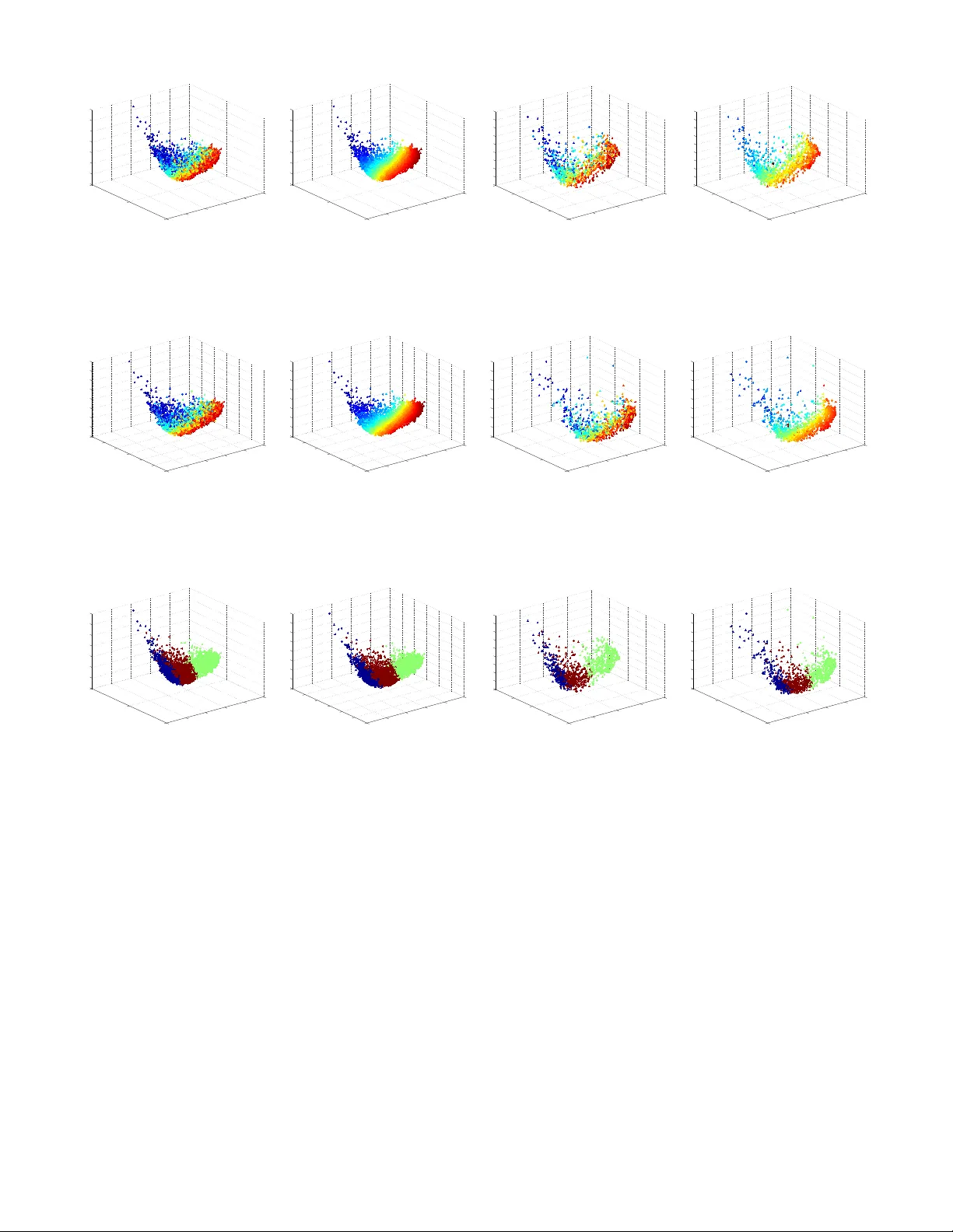
Auto-adaptativ e Laplacian Pyramids for High-dimensional Data Analysis ´ Angela F ern´ andez ∗ 1 , Neta Rabin † 2 , Dalia Fishelo v ‡ 2 and Jos ´ e R. Dorronsoro § 1 1 Dpto. Ing. Inform´ atica, UAM, 28049, Madrid, Spain 2 Dept. Exact Sciences, Afek a, T el-Aviv, 69107, Israel Abstract Non-linear dimensionalit y reduction techniques suc h as manifold learning algorithms hav e become a common w ay for processing and analyzing high-dimensional patterns that often ha v e attac hed a target that corresponds to the v alue of an unkno wn function. Their application to new p oin ts con- sists in tw o steps: first, embedding the new data p oin t into the lo w dimensional space and then, estimating the function v alue on the test p oin t from its neighbors in the embedded space. Ho wev er, finding the low dimension represen tation of a test p oin t, while easy for simple but often not pow erful enough pro cedures suc h as PCA, can be m uch more compli- cated for methods that rely on some kind of eigenanalysis, suc h as Spectral Clustering (SC) or Diffusion Maps (DM). Similarly , when a target function is to be ev aluated, av erag- ing metho ds lik e nearest neigh b ors ma y giv e unstable results if the function is noisy . Th us, the smo othing of the tar- get function with resp ect to the in trinsic, lo w-dimensional represen tation that describes the geometric structure of the examined data is a challenging task. In this pap er we prop ose Auto-adaptiv e Laplacian Pyra- mids (ALP), an extension of the standard Laplacian Pyra- mids mo del that incorp orates a mo dified Leav e One Out cross v alidation (LOOCV) pro cedure that av oids the large cost of standard LOOCV and offers the follo wing adv an- tages: (i) it selects automatically the optimal function res- olution (stopping time) adapted to the data and its noise, (ii) it is easy to apply as it do es not require parameteri- zation, (iii) it does not o verfit the training set and (iv) it adds no extra cost compared to other classical interpolation metho ds. W e illustrate numerically ALP’s behavior on a syn thetic problem and apply it to the computation of the DM pro jection of new patterns and to the extension to them ∗ a.fernandez@uam.es † netar@afek a.ac.il ‡ daliaf@post.tau.ac.il § jose.dorronsoro@uam.es of target function v alues on a radiation forecasting problem o ver very high dimensional patterns. Keyw ords: Laplacian Pyramids, LOOCV, Manifold Learning, Diffusion Maps. 1 Motiv ation An imp ortan t challenge in data mining and machine learn- ing is the prop er analysis of a given dataset, esp ecially for understanding and working with functions defined o ver it. In particular, manifold learning algorithms hav e b ecome a common wa y for pro cessing and analyzing high-dimensional data and the so called “diffusion analysis” allows us to find the most appropriate geometry to study such functions [25]. These metho ds are based on the construction of a diffusion op erator that dep ends on the lo cal geometry of the data, whic h is then used to embed the high-dimensional p oin ts in to a low er-dimensional space maintaining their geomet- ric properties and, hopefully , making easier the analysis of functions o ver it. On the other hand, extending functions in suc h an embedding for new data points may be c hallenging, either b ecause of the noise or the presence of lo w-density areas that mak e insufficient the num b er of a v ailable train- ing points. Also it is difficult to set the neighborho od size for new, unseen points as it has to be done according to the lo cal behavior of the function. The classical metho ds for function extension lik e Geomet- ric Harmonics [8] hav e parameters that need to b e carefully set, and in addition there does not exist a robust metho d of pic king the correct neigh b orhoo d in the em bedding for func- tion smo othing and ev aluation. A first attempt to simplify these approaches was Laplacian Pyramids (LP), a m ulti- scale mo del that generates a smo othed v ersion of a function in an iterativ e manner by using Gaussian k ernels of decreas- ing widths [21]. It is a simple metho d for learning functions from a general set of co ordinates and can be also applied to extend embedding co ordinates, one of the big challenges in diffusion methods. Recen tly [1] in tro duced a geometric PCA based out-of-sample extension for the purp ose of adding new p oin ts to a set of constructed embedding co ordinates. A na ¨ ıv e wa y to extend the target function to a new data p oin t could b e to find the point’s nearest neighbors (NN) in the embedded space and av erage their function v alues. The NN metho d for data lifting was compared in [12] with the LP version that w as prop osed in [21], and this last metho d performed b etter than NN. Buchman et al. [3] also describ ed a differen t, p oin t-wise adaptive approac h, whic h requires setting the nearest neighborho od radius parameter for every p oin t. Nev ertheless, and as it is often the case in machine learn- ing, when w e apply the previous LP mo del, w e can ov erfit the data if we try to refine to o muc h the prediction during the training phase. In fact, it is difficult to decide when to stop training to obtain goo d generalization capabilities. A usual approac h is to apply the Cross V alidation (CV) [13, c hap. 9] metho d to get a v alidation error and to stop when this error starts to increase. An extreme form of CV is the Lea ve One Out CV (LOOCV): a mo del is built using all 1 the samples but one, whic h is then used as a single v alida- tion pattern; this is repeated for each sample in the dataset, and the v alidation error is the av erage of all the errors. Al- though LOOCV has a theoretical backing and often yields go od results, it has the drawbac k of a big computational cost, though not in some imp ortan t cases (see Section 3). In this pap er we propose Auto-adaptive LP (ALP), a mo dification in the LP training algorithm that merges train- ing and approximate LOOCV in one single phase. T o do so w e simply build the k ernel matrix with zeros in its diago- nal. As we shall see, with this change we can implemen t an LOOCV approximation without any additional cost during the training step. This reduces significantly training com- plexit y and provides an automatic criterion to stop training so that we greatly a void the risk of sev ere ov erfitting that ma y app ear in standard LP . This effect can b e observ ed in Figure 1 when our LP prop osal is applied to the synthetic example used in Section 4. The solid and dashed black lines represen t the LP training error and the LOOCV error per iteration resp ectiv ely , and the dashed blue line represents the error for our prop osed method. The blue line, that cor- resp onds to the ALP training error attains its minimum at the same iteration prescrib ed by LOOCV for LP . k ALP = k LOOCV = 6 0 0 . 1 0 . 2 0 . 3 0 . 4 0 . 5 0 . 6 0 . 7 Iterations MAE ALP LP LOOCV Figure 1: T raining and LOOCV errors for the original and mo dified LP models applied to a synthetic example consist- ing on a p erturbed sine sho wn in Section 4. Therefore, ALP do esn’t ov erfit the data and, moreov er, do esn’t essen tially require an y parametrization or exp ert kno wledge ab out the problem, while still ac hieving a goo d test error. Moreo ver, it adds no extra cost compared to other classical neighbor-based interpolation metho ds. This pap er is organized as follows. In Section 2 w e briefly review the LP model and presen t a detailed analysis of its training error. W e describ e ALP in Section 3, which w e apply to a synthetic example in Section 4 and to a real w orld example in Section 5. The pap er ends with some conclusions in Section 6. 2 The Laplacian Pyramids The Laplacian Pyramid (LP) is an iterativ e mo del that w as in tro duced by Burt and Adelson [4] for its application in image pro cessing and, in particular, image enco ding. In the traditional algorithm, LP decomp oses the input image into a series of images, eac h of them capturing a differen t frequency band of the original one. This process is carried out by constructing Gaussian-based smo othing masks of different widths, follow ed b y a down-sampling (quan tization) step. LP was later pro ved to be a tigh t frame (see Do and V etterly [10]) and used for signal processing applications, for example as a reconstruction scheme in [19]. In [21], it was in tro duced a m ulti-scale algorithm in the spirit of LP to b e applied in the setting of high-dimensional data analysis. In particular, it was prop osed as a simple metho d for extending low-dimensional em b edding co ordi- nates that result from the application of a non-linear dimen- sionalit y reduction technique to a high-dimensional dataset (recen tly applied in [20]). W e review next the LP procedure as described in [21] (the do wn-sampling step, whic h is part of Burt and Adelson’s al- gorithm is skipp ed here). Let S = { x i } N i =1 ∈ R N b e the sam- ple dataset; the algorithm approximates a function f defined o ver S by constructing a series of functions { ˜ f i } obtained b y several refinemen ts d i o ver the error approximations. In a slight abuse of language we will use the same notation f for b oth the general function f ( x ) and also for the vector of its sample v alues f = ( f 1 = f ( x 1 ) , . . . , f N = f ( x N )). The result of this pro cess gives a function approximation f ' ˜ f = ˜ f 0 + d 1 + d 2 + d 3 + · · · In more detail, a first lev el k ernel K 0 σ ( x, x 0 ) = Φ (dist( x, x 0 ) /σ ) is chosen using a wide, initial scale σ and where dist( x, x 0 ) denotes some distance function betw een p oin ts in the original dataset. A usual choice and the one w e will use here is the Gaussian k ernel with Euclidean dis- tances, i.e., to take dist( x, x 0 ) = k x − x 0 k and then K 0 ( x, x 0 ) = κe − k x − x 0 k 2 σ 2 , where κ is the Gaussian k ernel normalizing constan t. As be- fore, w e will use the K 0 notation for both the general con tin- uous k ernel K 0 ( x, x 0 ) and for its discrete matrix coun terpart K (0) j k = K 0 ( x j , x k ) ov er the sample p oin ts. The smo othing operator P 0 is constructed as the normal- ized row-stochastic matrix of the kernel P 0 ij = K 0 ij P k K 0 ik . (1) A first coarse representation of f is then generated b y the con volution ˜ f 0 = f ∗ P 0 that captures the low-frequencies of the function. F or the next steps we fix a µ > 1, construct at step i a sharper Gaussian kernel P i with scale σ /µ i , and the residual d i − 1 = f − ˜ f i − 1 , 2 whic h captures the error of the appro ximation to f at the previous i − 1 step, is used to generate a more detailed rep- resen tation of f given b y ˜ f i = ˜ f i − 1 + d i − 1 ∗ P i = ˜ f i − 1 + g i − 1 , with g ` = d ` ∗ P ` +1 . The iterativ e algorithm stops once the norm of d i residual vector is smaller than a predefined error. Stopping at iteration L , the final LP mo del has th us the form ˜ f L = ˜ f 0 + L − 1 X 0 g ` = f ∗ P 0 + L − 1 X 0 d ` ∗ P ` +1 , (2) and extending this m ulti-scale represen tation to a new data p oin t x ∈ R N is now straightforw ard b ecause we simply set ˜ f L ( x ) = f ∗ P 0 ( x ) + L − 1 X 0 d ` ∗ P ` +1 ( x ) = X j f j P 0 ( x, x j ) + L X 1 X j d ` − 1; j P ` ( x, x j ) . where we extend the P ` k ernels to a new x as P ` ( x, x j ) = K ` ( x, x j ) P k K ` ( x, x k ) . The o verall cost is easy to analyze. Computing the con v o- lutions ˜ f 0 = f ∗ P 0 , g ` = d ` ∗ P ` − 1 has a O ( N 2 ) cost for a size N sample, while that of obtaining the d ` is just O ( N ). Th us, the ov erall cost of L LP steps is O ( LN 2 ). W e observe that if we set a very small error threshold and run afterw ards enough iterations, w e will end up having ˜ f ` = f ov er the training sample. In fact, ˜ f ` = ˜ f ` − 1 + g ` − 1 and, therefore, ˜ f ` = ˜ f ` − 1 + g ` − 1 = ˜ f ` − 1 + ( f − ˜ f ` − 1 ) ∗ P ` = f ∗ P ` + ˜ f ` − 1 ∗ ( I − P ` ) , with I denoting the identit y matrix. Now, if we hav e ˜ f ` → φ , it follows taking limits that φ = f ∗ lim P ` + φ ∗ lim( I − P ` ) i.e., φ = f , for P ` → I . In practice, w e will numerically hav e P ` = I as soon as ` is large enough so that w e hav e K ` ( x i , x j ) ' 0. W e then ha ve d ` ; j = 0 for all j and the LP mo del doesn’t c hange anymore. In other words, care has to b e taken when deciding to stop the LP iterations to av oid o verfitting. In fact, we show next that when using Gaussian k ernels, as we do, the L 2 norm of the LP errors ˆ d ` deca y extremely fast. First notice that w orking in the con tinuous k ernel setting, w e hav e P = K for a Gaussian kernel, for then the denomi- nator in (1) is just R K ( x, z ) dz = 1. Assume that f is in L 2 , so R x f 2 ( x ) dx < ∞ . The LP scheme is a relaxation pro cess for which in the first step the function f is approximated b y G 0 ( f ) = f ∗ P 0 ( x ). F or all ` , P ` ( x ) is an approximation to a delta function satisfying Z P ` ( x ) dx = 1 , Z xP ` ( x ) dx = 0 , (3) Z x 2 P ` ( x ) dx ≤ 2 C. In the second step f is approximated by G 0 ( f ) + G 1 ( d 0 ), where d 0 = G 0 ( f ) − f and G 1 ( d 0 ) = d 0 ∗ P 1 ( x ), and so on. T aking the F ourier transform of P ` ( x ), we ha ve (see [15])    ˆ P ` ( ω )    ≤ 1 + σ 2 2 Z x 2 P ` ( x ) dx ≤ 1 + C σ 2 , (4) where we ha ve used (3). W e first analyze the error d 0 ( x ) in the first step, which is defined by d 0 ( x ) = f ∗ P 0 ( x ) − f . T aking the F ourier transform of d 0 ( x ) and using (4) we hav e    ˆ d 0 ( ω )    =    ˆ f ( w )       ˆ P 0 ( ω ) − 1    ≤ C σ 2 0    ˆ f ( ω )    . (5) The error in the second step is d 1 ( x ) = d 0 − G 1 ( d 0 ) =  f ∗ P 0 − f  − d 0 ∗ P 1 . (6) T aking the F ourier transform of (6) yields    ˆ d 1 ( ω )    =    ˆ d 0 ( ω ) − ˆ d 0 ( ω ) ˆ P 1 ( ω )    =    ˆ d 0 ( ω )       ˆ P 1 ( ω ) − 1    . Using (4) and (5) we obtain    ˆ d 1 ( ω )    ≤ C    ˆ d 0 ( ω )    σ 2 1 ≤ C σ 2 0 σ 2 1    ˆ f ( ω )    . Since σ 1 = σ 0 µ with µ > 1, then    ˆ d 1 ( ω )    ≤ C σ 2 0 σ 2 0 µ 2    ˆ f ( ω )    . Similarly , for the ` th step the error is b ounded b y    ˆ d ` ( ω )    ≤ C σ 2 0  σ 2 0 µ 2  `    ˆ f ( ω )    . By Parsev al’s equality we obtain k d ` k L 2 ≤ C σ 2 0  σ 2 0 µ 2  ` k f k L 2 . Th us, the error’s L 2 deca ys faster than any algebraic rate. W e see next ho w we can estimate a final iteration v alue L that preven ts ov erfitting without incurring on additional costs. 3 Auto-adaptativ e Laplacian Pyra- mids The standard w ay to preven t ov erfitting is to use an indep en- den t v alidation subset and to stop the ab o v e ` iterations as 3 so on as the v alidation error on that subset starts to increase. This can b e problematic for small samples and introduces a random dependence on the c hoice of the particular v alida- tion subset; k -fold cross v alidation is then usually the stan- dard c hoice, in which w e randomly distribute the sample in k subsets, and iteratively use k − 1 subsets for training and the remaining one for v alidation. In the extreme case when k = N , i.e., we use just one pattern for v alidation, we ar- riv e at Lea ve One Out Cross V alidation (LOOCV) and stop the training iterations when the LOOCV error starts to in- crease. Besides its simplicity , LOOCV has the attractive of b eing an almost unbiased estimator of the true generaliza- tion error (see for instance [5, 14]), although with possibly a high v ariance [18]. In our case LOOCV can b e easily ap- plied using for training a N × N normalized k ernel matrix P ( p ) whic h is just the previous matrix K where w e set to 0 the p -th ro ws and columns when x p is held out of the training sample and used for v alidation. The most ob vious dra wback of LOOCV is its rather high cost, which in our case is N × O ( LN 2 ) = O ( LN 3 ) cost. Ho wev er, it is often the case for other mo dels that there are wa ys to estimate the LOOCV error with a smaller cost. This can b e done exactly in the case of k -Nearest Neighbors [16] or of Ordi- nary Least Squares ([17], Chapter 7), or approximately for Supp ort V ector Machines [6] or Gaussian Pro cesses [22]. In order to alleviate it, notice first that when we remo ved x p from the training sample, the test v alue at x p of the f ( p ) extension built is f ( p ) L ( x p ) = X j 6 = p f j P 0 ( x p , x j ) + L X ` =1 X j 6 = p d ( p ) ` − 1; j P ` ( x p , x j ) = X j f j ˜ P 0 ( x p , x j ) + L X ` =1 X j d ( p ) ` − 1; j ˜ P ` ( x p , x j ) , where d ( p ) ` are the different errors computed using the P ` ( p ) matrices and where ˜ P is now just the matrix P with its diagonal elements set to 0, i.e. ˜ P i,i = 0, ˜ P i,j = P i,j when j 6 = i . This observ ation leads to the modification we propose on the standard LP algorithm giv en in [21], and which simply consist on applying the LP pro cedure described in Section 2 but replacing the P matrix by its 0-diagonal version ˜ P , computing then ˜ f 0 = f ∗ ˜ P 0 at the b eginning, and ˜ d ` = f − ˜ f ` , ˜ g ` = ˜ d ` ∗ ˜ P ` +1 and ˜ f ` v ectors at each iteration. W e call this algorithm the Auto-adaptative Laplacian Pyramid (ALP). According to the previous form ula for the f ( p ) L ( x p ), w e can take the ALP v alues ˜ f L,p = ˜ f L ( x p ) given b y ˜ f L ( x p ) = X j f j ˜ P 0 ( x p , x j ) + L X ` =1 X j ˜ d ` − 1; j ˜ P ` ( x p , x j ) , as approximations to the LOOCV v alidation v alues f ( p ) L ( x p ). But then we can appro ximate the square LOOCV error at iteration L as X p ( f ( x p ) − f ( p ) L ( x p )) 2 ' X p ( f ( x p ) − ˜ f L,p ) 2 = X p ( ˜ d L ; p ) 2 , whic h is just the training error of ALP . In other w ords, w ork- ing with the ˜ P matrix instead of P , the training error at step L giv es in fact an appro ximation to the LOOCV error at this step. The cost of running L steps of ALP is just O ( LN 2 ) and, thus, we gain the adv antage of the exhaustiv e LOOCV without an y additional cost on the ov erall algorithm. The complete training pro cedure is presen ted in Algorithm 1 and the test algorithm is shown in Algorithm 2. Algorithm 1 The ALP T raining Algorithm Input: x tr , y tr , σ 0 , µ . Output: ( { d i } , σ 0 , µ, k ) % The trained model. 1: σ ← σ 0 ; d 0 ← y tr . 2: ˜ f 0 ← 0; i ← 1. 3: while (err i < err i − 1 ) do 4: K ← e − k x tr − x tr k 2 / σ 2 . 5: P i ← normalize( K ). 6: ˜ P ← P with 0-diagonal. % LOOCV. 7: ˜ f i ← ˜ f i − 1 + d i − 1 ∗ ˜ P i . 8: d i ← f − ˜ f i . 9: err i ← d i / s tr , with s tr the num b er of patterns in x tr . 10: σ ← σ / µ ; i ← i + 1. 11: end while 12: k ← min i d i . % Optimal iteration. Algorithm 2 The ALP T esting Algorithm Input: x tr , x te , ( { d i } , σ 0 , µ, k ). Output: ˆ y te . 1: ˆ y te ← 0; σ ← σ 0 . 2: for i=0 to k-1 do 3: K ← e − k x tr − x te k 2 / σ 2 . 4: P i ← normalize( K ). 5: ˆ y te ← ˆ y te + d i ∗ P i . 6: σ ← σ / µ . 7: end for The ob vious adv antage of ALP is that when we ev aluate the training error, w e are actually estimating the LOOCV error after each LP iteration. Therefore, the evolution of these LOOCV v alues tells us which is the optimal iteration to stop the algorithm, i.e., just when the training error ap- pro ximation to the LOOCV error starts growing. Thus, w e do not only remo ve the danger of o verfitting but can also use the training error as an approximation to the generalization error. This effect can be seen in Figure 1 whic h illustrates the application of ALP to the syn thetic problem describ ed in the next section and where the optimum stopping time for ALP is exactly the same that the one that would give the LOOCV error and where training error stabilizes afterw ards at a slightly larger v alue. Moreo ver, ALP ac hieves an automatic selection of the width of the Gaussian k ernel whic h mak es this v ersion of LP to be auto-adaptative as it do es not require costly param- eter selection procedures. In fact, c ho osing as customarily done µ = 2, the only required parameter w ould be the ini- tial σ but provided it is wide enough, its σ/ 2 ` scalings will yield an adequate final kernel width. 4 A Syn thetic Example F or a b etter understanding of this theory , we first illustrate the prop osed ALP algorithm on a synthetic example of a 4 0 5 10 15 20 25 30 35 − 1 . 5 − 1 − 0 . 5 0 0 . 5 1 1 . 5 XT est Iteration 1 0 5 10 15 20 25 30 35 − 1 . 5 − 1 − 0 . 5 0 0 . 5 1 1 . 5 XT est Iteration 2 0 5 10 15 20 25 30 35 − 1 . 5 − 1 − 0 . 5 0 0 . 5 1 1 . 5 XT est Iteration 3 0 5 10 15 20 25 30 35 − 1 . 5 − 1 − 0 . 5 0 0 . 5 1 1 . 5 XT est Iteration 4 0 5 10 15 20 25 30 35 − 1 . 5 − 1 − 0 . 5 0 0 . 5 1 1 . 5 XT est Iteration 5 0 5 10 15 20 25 30 35 − 1 . 5 − 1 − 0 . 5 0 0 . 5 1 1 . 5 XT est Iteration 6 0 5 10 15 20 25 30 35 − 1 . 5 − 1 − 0 . 5 0 0 . 5 1 1 . 5 XT est Iteration 7 Figure 2: Ev olution of the Auto-adaptative Laplacian Pyramids mo del for the first example. comp osition of sines with differen t frequencies plus additive noise. W e consider a sample x with N p oin ts equally spaced o ver the range [0 , 10 π ]. The target function f is then f = sin( x ) + 0 . 5 sin(3 x ) · I 2 ( x ) + 0 . 25 sin(9 x ) · I 3 ( x ) + ε, where I 2 is the indicator function of the in terv al (10 π / 3 , 10 π ], I 3 that of (2 · 10 π / 3 , 10 π ] and ε ∼ U ([ − δ, δ ]) is uniformly distributed noise. In other words, we hav e a sin- gle frequency in the interv al [0 , 10 π / 3], t wo frequencies in (10 π / 3 , 2 · 10 π / 3] and three in (2 · 10 π / 3 , 10 π ]. W e run tw o differen t simulations, the first one with 4 , 000 p oin ts with small δ = 0 . 05 noise and the second one with 2 , 000 points and a larger δ = 0 . 25 (observe that | f | ≤ 1 . 75). In b oth cases, o dd indexed p oin ts form the training set and even p oin ts form the test set. Recall that the ALP model automatically adapts its mul- tiscale b eha vior to the data, trying to refine the prediction in each iteration using a more lo calized k ernel, given b y a smaller σ . This b eha vior can be observed in Figure 2, whic h sho ws the evolution of the prediction of the ALP for small noise exp erimen t. As w e can see, at the b eginning, the mo del approximates the function just b y a coarse mean of the target function v alues; how ever in the subsequent itera- tions that start using sharp er kernels and refined residuals, the appro ximating function starts capturing the different frequencies and amplitudes of the comp osite sines. In this particular case the minimum LOOCV v alue is reached after 7 iterations, a relatively small n umber which mak es sense as w e hav e a simple mo del with small noise. When w e rep eat the same synthetic exp erimen t but now enlarging the amplitude of the uniform distribution to δ = 0 5 10 15 20 25 30 35 − 2 − 1 . 5 − 1 − 0 . 5 0 0 . 5 1 1 . 5 XT est T arget Prediction Figure 3: Prediction of the Auto-adaptativ e Laplacian Pyra- mids mo del for the second example. 0 . 25, the predicted function is represented in Figure 3 and it is obtained after 6 iterations. As it w as to be exp ected, the num b er of LP iterations is now slightly smaller than in the previous example b ecause the algorithm selects a more conserv ative, smo other prediction in the presence of noisier and, thus, more difficult data. In any case, w e can conclude that the ALP model captures 5 v ery well the essential b eha vior underlying both samples, catc hing the three differen t frequencies of the sine and their amplitudes even when the noise level increases. 5 ALP for Eigen v ector Estimation in Sp ectral Clustering and Diffu- sion Maps 5.1 Spectral Manifold Learning A common assumption in many big data problems is that al- though original data appear to hav e a very large dimension, they lie in a low dimensional manifold M of which a suit- able representation has to be giv en for adequate mo deling. Ho w to iden tify M is the key problem in manifold learning, where the preceding assumption has giv en rise to a num b er of methods among which we can men tion Multidimensional Scaling [9], Local Linear Em b edding [23], Isomap [26], Spec- tral Clustering (SC) [24] and its sev eral v ariants such as Laplacian Eigenmaps [2], or Hessian eigenmaps [11]. Diffu- sion methods (DM) [7] also follo w this set up and w e cen ter our discussion on them. The k ey assumption in Diffusion methods is that the met- ric of the low dimensional Riemannian manifold where data lie can b e appro ximated by a suitably defined diffusion met- ric. The starting p oin t in DM (and in SC) is a w eighted graph representation of the sample with a similarity ma- trix w ij giv en by the kernel e − k x i − x j k 2 / 2 σ 2 . In order to con trol the effect of the sample distribution, a parameter α ∈ [0 , 1] is introduced in DM and w e work instead with the α -dep enden t similarity w ( α ) ij = w ij / g α i g α j , where g i = P j w ij is the degree of v ertex i . The new vertex degrees are now g α i = P j w α ij and we define a Marko v transition matrix ˜ W ( α ) = { ˜ w ( α ) ij = w ( α ) ij / g α i } . Fixing the num b er t of steps considered in the Mark o v pro cess, w e can tak e into account t neigh b ors of an y p oin t in terms of the t -step diffusion dis- tance given b y D t ij = k ˜ w ( α ; t ) i, · − ˜ w ( α ; t ) j, · k L 2 ( 1 / φ 0 ) , where φ 0 is the stationary distribution of the Marko v pro cess and ˜ w ( α ; t ) the transition probability in t steps (i.e., the t -th p o wer of ˜ w α ). W e will w ork with t = 1 and use α = 1. As it is sho wn in [7], when α = 1, the infinitesimal generator L 1 of the diffusion pro cess coincides with the manifold’s Laplace– Beltrami op erator ∆ and, thus, we can exp ect the diffusion pro jection to capture the underlying geometry . No w, the eigenanalysis of the Marko v matrix ˜ W ( α ) giv es an alternative represen tation of the diffusion distance as D t ij = X k λ 2 t k ( ψ ( k ) i − ψ ( k ) j ) 2 , with λ k the eigenv alues and ψ ( k ) the left eigen vectors of the Mark ov matrix ˜ W ( α ) and ψ ( k ) i = ψ k ( x i ) are the eigenv ec- tors’ comp onen ts [7]. The eigenv alues λ k deca y rather fast, a fact w e can use to p erform dimensionalit y reduction by setting a fraction δ of the second eigenv alue λ 1 (the first one λ 0 is alwa ys 1 and carries no information) and retaining th us a num b er d = d t of those λ k for which λ t k > δ λ t 1 . This δ is a parameter w e ha ve to c ho ose besides the previous α and t . Usual v alues are either δ = 0 . 1 or the more strict (and larger dimension inducing) δ = 0 . 01. Once fixed, we w ould thus arriv e to the diffusion co ordinates Ψ =    λ t 1 ψ 1 ( x ) . . . λ t d ψ d ( x )    and we can approximate the diffusion distance as D t ij ∼ d X 1 λ t k ( ψ k i − ψ k j ) 2 = k Ψ( x i ) − Ψ( x j ) k 2 . In other w ords, the diffusion distance in M can b e appro x- imated b y Euclidean distance in the DM pro jected space. This makes DM a v ery useful to ol to apply procedures in the pro jected space suc h as K -means clustering that usually rely on an implicit Euclidean distance assumption. All the steps to compute DM are summarized in Algorithm 3. While very elegant and p o w erful, DMs hav e the draw- bac k of relying on the eigenv ectors of the Marko v matrix. This makes it difficult to compute the DM co ordinates of a new, unseen pattern x . Moreov er, the eigenanalysis of the ˜ W ( α ) matrix would ha ve in principle a p oten tially very high O ( N 3 ) cost, with N sample’s size. How ev er, b oth issues can b e addressed in terms of function appro ximation. The stan- dard approach is to apply the Nystr¨ om extension formula [27] but LPs [21] and, hence, ALPs, can also b e used in this setting, as we discuss next. T o do so we consider the eigen v alue comp onen ts ψ ( k ) j as the v alues ψ ( k ) ( x j ) at the p oin ts x j of an unkno wn function ψ ( k ) ( x ) which we try to appro ximate by an ALP sc heme. The general LP formula (2) for the eigen vector ˆ ψ ( k ) ex- tended to an out-of-sample p oin t x b ecomes no w ˆ ψ ( k ) ( x ) = ψ ( k ) ∗ P 0 ( x ) + L − 1 X 0 d ` ∗ P ` +1 ( x ) = N X i =1 P 0 ( x, x i ) ψ ( k ) ( x i ) + H X h =1 N X i =1 P h ( x, x i ) d ( k ) h ( x i ) , (7) with the differences d ( k ) h giv en now by d ( k ) h ( x i ) = ψ ( k ) ( x i ) − P h − 1 ` =0 ˆ ( ψ ( k ) ) ( ` ) ( x i ). W e illustrate next the application of these techniques to the analysis of solar radiation data where we relate actual aggregated radiation v alues with Numerical W eather Pre- diction (NWP) v alues. 5.2 Diffusion Maps of Radiation Data A current imp ortan t problem that is getting a gro wing at- ten tion in the Machine Learning comm unity is the predic- tion of renewable energies, particularly solar energy and, therefore, of solar radiation. W e will consider here the pre- diction of the total daily incoming solar energy in a series 6 Algorithm 3 Diffusion Maps Algorithm. Input: S = { x 1 , . . . , x N } , the original dataset. P arameters: t , α , σ , δ . Output: { Ψ( x 1 ) , . . . , Ψ( x N ) } , the embedded dataset. 1: Construct a graph G = ( S , W ) where W ij = w ( x i , x j ) = e −k x i − x j k 2 2 σ 2 . 2: Define the initial densit y function as g ( x i ) = N X j =1 w ( x i , x j ) . 3: Normalize the weigh ts by the density: w ( α ) ( x i , x j ) = w ( x i , x j ) g α i g α j . 4: Define the transition probabilit y ˜ W ( α ) ij = ˜ w ( α ) ( x i , x j ) = ˜ w ( α ) ( x i , x j ) g ( α ) i , where g ( α ) i = P n j =1 w ( α ) ( x i , x j ) is the graph degree. 5: Obtain eigenv alues { λ r } r > 0 and eigenfunctions { ψ r } r > 0 of ˜ W ( α ) suc h that  1 = λ 0 > | λ 1 | > · · · ˜ W ( α ) ψ r = λ r ψ r . 6: Compute the embedding dimension using a threshold d = max { ` : | λ ` | > δ | λ 1 |} . 7: F ormulate Diffusion Map: Ψ =    λ t 1 ψ 1 ( x ) . . . λ t d ψ d ( x )    . of meteorological stations lo cated in Oklahoma in the con- text of the AMS 2013-2014 Solar Energy Prediction Con test hosted b y the Kaggle company . 1 While the ultimate goal w ould be here to obtain b est predictions, we will use the problem to illustrate the application of ALP in the previ- ously describ ed DM setting. The input data are an ensemble of 11 numerical weather predictions (NWP) from the NO AA/ESRL Global Ensem- ble F orecast System (GEFS). W e will just use the main NWP ensemble as b eing the one with the highest probabil- it y of b eing correct. Input patterns contain five time-steps (from 12 to 24 UCT-hours in 3 hour incremen ts) with 15 v ariables per time-step for all p oin ts in a 16 × 9; eac h pat- 1 American Meteorological So ciet y 2013-2014 Solar En- ergy Prediction Contest ( https://www.kaggle.com/c/ ams- 2014- solar- energy- prediction- contest ). tern has thus a very large 10 , 800 dimension. The NWP forecasts from 1994–2004 yield 4 , 018 training patters and the y ears 2005, 2006 and 2007, with 1 , 095 patterns, are used for testing. Our first goal is to illustrate how applying ALP results in go od approximations to the DM co ordinates of new p oin ts that were not av ailable for the first eigenanalysis of the ini- tial Marko v matrix. T o do so, we normalize training data to 0 mean and a standard deviation 1 and use the DM ap- proac h explained ab o ve, working with a Gaussian kernel, whose σ parameter has b een established as the 50% p er- cen tile of the Euclidean distances betw een all sample points. W e recall that w e fix the diffusion step t to 1 and also the α parameter, so that data densit y do es not influence diffusion distance computations. T o decide the b est dimensionality for the embedding, the precision parameter δ has b een fixed at a relativ ely high v alue of 0 . 1, i.e., w e only k eep the eigen- v alues that are bigger than the 10% of the first non trivial eigen v alue. This c hoice yields an em b edding dimension of 3, whic h enables to visualize the results. W e apply DM with these parameters o ver the training set and obtain the corre- sp onding eigenv ectors, i.e., the sample v alues ψ ( k ) ( x i ) ov er the training patterns x i , and the DM co ordinates of the training points. W e then apply Algorithm 1 to decide on the ALP stopping iteration and to compute the differences d ( k ) h ( x i ) in (7) and finally apply Algorithm 2 to obtain the appro ximations to the v alues of ψ ( k ) o ver the test p oin ts. In order to measure the go o dness of the new co ordinates, w e hav e also performed the DM eigenanalysis to the entire NWP data, i.e., to the training and test inputs together. In this w ay we can compare the extended em b edding obtained using ALP with the one that would ha v e b een obtained if w e had known the correct diffusion co ordinates. 5.3 Results F or this exp erimen ts the results hav e b een obtained com- puting a DM em b edding only o ver the training sample, and using ALP first to extend DM to the test sample and then for radiation prediction. In Figure 5 training and test results are shown. The three diffusion coordinates for this example are colored by the target, i.e. by the solar radiation (first and third), or by the prediction given b y ALP (second and fourth). In the first and third image we can see that DM captures the structure of the target radiation in the sample, with the low radiation data (blue) app earing far apart from the points with high radiation (red). If w e compare this with the prediction-colored embeddings (second and fourth) w e can observ e that the radiation v alues hav e b een smo othed across color bands and that the general radiation trend is captured approximately along the second DM feature even if not every detail is mo deled (recall that measured radi- ation is the target v alue and, thus, is not included in the DM transformation). This b eha vior can be observ ed for the training p oin ts in first and second plots but also for the test ones in the third and fourth ones, where it can b e seen that the ALP metho d mak es a goo d extension of the target function for new p oin ts. F or comparison purp oses training and test ALP results 7 −0.015 −0.01 −0.005 0 0.005 0.01 −5 0 5 x 10 −3 −2 −1 0 1 2 3 4 5 x 10 −3 ψ 1 ψ 2 ψ 3 (a) T raining Radiation. −0.015 −0.01 −0.005 0 0.005 0.01 −5 0 5 x 10 −3 −2 −1 0 1 2 3 4 5 x 10 −3 ψ 1 ψ 2 ψ 3 (b) T raining ALP Prediction. −0.01 −0.005 0 0.005 0.01 −4 −2 0 2 4 x 10 −3 −1.5 −1 −0.5 0 0.5 1 1.5 2 2.5 3 x 10 −3 ψ 1 ψ 2 ψ 3 (c) T est Radiation. −0.01 −0.005 0 0.005 0.01 −4 −2 0 2 4 x 10 −3 −1.5 −1 −0.5 0 0.5 1 1.5 2 2.5 3 x 10 −3 ψ 1 ψ 2 ψ 3 (d) T est ALP Prediction. Figure 4: T raining and test results when the DM embedding is computed ov er the en tire sample and ALP used only for radiation prediction. −0.015 −0.01 −0.005 0 0.005 0.01 −6 −4 −2 0 2 4 6 x 10 −3 −2 −1 0 1 2 3 4 5 6 x 10 −3 ψ 1 ψ 2 ψ 3 (a) T raining Radiation. −0.015 −0.01 −0.005 0 0.005 0.01 −6 −4 −2 0 2 4 6 x 10 −3 −2 −1 0 1 2 3 4 5 6 x 10 −3 ψ 1 ψ 2 ψ 3 (b) T raining ALP Prediction. −0.015 −0.01 −0.005 0 0.005 0.01 −5 0 5 10 x 10 −3 −2 −1 0 1 2 3 4 5 6 x 10 −3 ψ 1 ψ 2 ψ 3 (c) T est Radiation. −0.015 −0.01 −0.005 0 0.005 0.01 −5 0 5 10 x 10 −3 −2 −1 0 1 2 3 4 5 6 x 10 −3 ψ 1 ψ 2 ψ 3 (d) T est ALP Prediction. Figure 5: T raining and test results when the DM embedding is computed only on the training sample and ALP is used first to extend DM to the test sample and then for radiation prediction. −0.015 −0.01 −0.005 0 0.005 0.01 −5 0 5 x 10 −3 −2 −1 0 1 2 3 4 5 x 10 −3 ψ 1 ψ 2 ψ 3 (a) T raining DM F ull. −0.015 −0.01 −0.005 0 0.005 0.01 −6 −4 −2 0 2 4 6 x 10 −3 −2 −1 0 1 2 3 4 5 6 x 10 −3 ψ 1 ψ 2 ψ 3 (b) DM T raining Sample. −0.01 −0.005 0 0.005 0.01 −4 −2 0 2 4 x 10 −3 −1.5 −1 −0.5 0 0.5 1 1.5 2 2.5 3 x 10 −3 ψ 1 ψ 2 ψ 3 (c) T est DM F ull. −0.015 −0.01 −0.005 0 0.005 0.01 −5 0 5 10 x 10 −3 −2 −1 0 1 2 3 4 5 6 x 10 −3 ψ 1 ψ 2 ψ 3 (d) T est Expanded by ALP . Figure 6: Clusters ov er the embedded data. when the DM embedding is computed o v er the entire sample are shown in Figure 4 (we could consider this as the “true” DM em b edding). Comparing with Figure 5 we can see that the t wo DM embeddings are very similar and that the target and prediction colors seem to b e more or less the same. This shows that when w e apply ALP to compute the DM co ordinates of new test sample points w e get an em b edding quite close to the ideal one obtained join tly ov er the train and test patterns. In order to giv e a quan titative measure of the qualit y of the ALP pro jections, we p erform Euclidean K -means with K = 3 ov er the three-dimensional embeddings of the test sample. W e wan t to compare the clusters obtained o ver the ideal DM embedding computed with the entire sample and the ones obtained ov er the train DM embedding and then extended for the test co ordinates. The resulting clusterings can b e seen in figure 6. Notice that these clusters do not re- flect radiation structure; instead more weigh t is apparently giv en to the first DM feature (that should ha ve the largest feature v alues and, thus, a bigger influence when Euclidean distances are computed). Anyw ay , recall that this embed- ding was made with 15 different v ariable types, from which just 5 are radiation v ariables. Because of this, the cluster structure doesn’t hav e to reflect just radiation’s effect on the embedding, but the ov erall v ariable b eha vior. T o obtained a concrete metric w e will compare the cluster assignmen ts of the test p oin ts o ver the extended em b edding (the “predicted” assignments) with those made ov er the full em b edding (the “true” assignmen ts). Lo oking at this as a classification problem, the accuracy , i.e., the p ercen tage of test p oin ts assigned to their “real” clusters, measures how w ell the ALP extensions matc h the “true” em b edding struc- ture. As the confusion matrix in T able 1 sho ws, ALP do es this quite well, with a total accuracy of 97 . 53%. Thus, if clustering of the embedded features is desired, ALP mak es it p ossible for new patterns with a v ery high accuracy . 8 T able 1: Confusion Matrix of the K -means classification for the extended test co ordinates. P . 1 P . 2 P . 3 P R. 1 294 4 0 298 R. 2 9 342 2 353 R. 3 0 12 432 444 P 303 358 434 1095 Getting bac k to radiation prediction ov er the test sample, once the embedding is obtained, we try to predict o ver it the total daily incoming solar energy using no w a tw o step ALP pro cedure. T o do so, DM are applied o ver the training sample to obtain the DM em b edded features and then a first ALP mo del ALP F is built to extend the DM features to the test sample and a second ALP ALP R to build the ALP function appro ximation to the target radiation. Given a new NWP test pattern, w e apply ALP F to obtain its extended DM features and, next, ALP R o ver them to obtain the final radiation prediction. In Figure 8, left, w e ha ve depicted for the second test y ear the real radiation in light blue and the ALP prediction in dark blue. Although the winning mo dels in the Kaggle comp etition follow ed different approaches, it can b e seen that ALP captures radiation’s seasonalit y . In the righ t plot w e zoom in and it can b e appreciated how ALP tracks the radiation v ariations. Even if not ev ery peak is caugh t, ALP yields a reasonably go od approximation to actual radiation without requiring any particular parameter choices nor an y exp ert knowledge ab out the problem w e wan ted to address. Figure 7 sho ws the ev olution of standard LP training error, its associated LOOCV error and the LOOCV estimation giv en by ALP when they are applied for radiation forecast- ing. It illustrates the robustness of the ALP mo del against o verfitting. Again, the ALP model requires here the same n umber of 15 iterations suggested by applying full LOOCV to standard LP . Finally , Figure 9 shows for a test p oin t x , plotted as a blac k dot, the ev olution as ALP adv ances of the influence of sample p oin ts on x , larger for red p oin ts and smaller for blue ones. As it can b e seen, as σ gets smaller, the num b er of high influence red p oin ts also decreases sharply and so do es the p ossibilit y of ov erfitting. 6 Conclusions The classical Laplacian Pyramid scheme of Burt and Adel- son ha ve b een widely studied and applied to man y problems, particularly in image pro cessing. Ho wev er, it has the risk of ov erfitting and, thus, requires the use of rather costly tec hniques such as cross v alidation to preven t it. In this paper we hav e presen ted Auto-adaptative Lapla- cian Pyramids (ALP), a mo dified, adaptive version of LP training that yields at no extra cost an estimate of the k ALP = k LOOCV = 15 0 0 . 1 0 . 2 0 . 3 0 . 4 0 . 5 0 . 6 0 . 7 0 . 8 0 . 9 Iterations MAE T rain ALP T rain LP LOOCV Figure 7: T raining error for the solar example of ALP , stan- dard LP and its asso ciated LOOCV. − 2 . 5 − 2 − 1 . 5 − 1 − 0 . 5 0 0 . 5 1 1 . 5 2 Normalized radiation T arget Prediction Figure 8: Prediction of the daily incoming solar energy ov er the second test year, and in a zo om ov er 100 days. LOOCV v alue at each iteration, allo wing thus to automati- cally decide when to stop in order to av oid ov erfitting. W e ha ve illustrated the robustness of the ALP metho d o ver a syn thetic example and sho wn on a real radiation problem ho w to use it to extend Diffusion Maps embeddings to new patterns and to provide simple, yet reasonably goo d radia- tion predictions. Ac kno wledgments The authors wish to thank Prof. Y o el Shkolnisky and Prof. Ronald R. Coifman for helpful remarks. The first author ac- kno wledge partial supp ort from grant TIN2010-21575-C02- 01 of Spain’s Ministerio de Econom ´ ıa y Comp etitividad and the UAM–ADIC Chair for Mac hine Learning in Mo deling and Prediction. References [1] Y. Aizenbud, A. Bermanis, and A. Av erbuch. PCA- based out-of-sample extension for dimensionalit y re- duction. Submitted. http://www.cs.tau.ac.il/ ~ amir1/PS/pbe.pdf . 9 −12 −10 −8 −6 −4 −2 0 2 4 6 8 x 10 −3 −5 −4 −3 −2 −1 0 1 2 3 4 5 x 10 −3 ψ 1 ψ 2 −12 −10 −8 −6 −4 −2 0 2 4 6 8 x 10 −3 −5 −4 −3 −2 −1 0 1 2 3 4 5 x 10 −3 ψ 1 ψ 2 −12 −10 −8 −6 −4 −2 0 2 4 6 8 x 10 −3 −5 −4 −3 −2 −1 0 1 2 3 4 5 x 10 −3 ψ 1 ψ 2 −12 −10 −8 −6 −4 −2 0 2 4 6 8 x 10 −3 −5 −4 −3 −2 −1 0 1 2 3 4 5 x 10 −3 ψ 1 ψ 2 −12 −10 −8 −6 −4 −2 0 2 4 6 8 x 10 −3 −5 −4 −3 −2 −1 0 1 2 3 4 5 x 10 −3 ψ 1 ψ 2 −12 −10 −8 −6 −4 −2 0 2 4 6 8 x 10 −3 −5 −4 −3 −2 −1 0 1 2 3 4 5 x 10 −3 ψ 1 ψ 2 Figure 9: Ev olution of the neighborho od of a test p oin t ov er the embedded training p oin ts. [2] M. Belkin and P . Ny ogi. Laplacian Eigenmaps for di- mensionalit y reduction and data represen tation. Neur al Computation , 15(6):1373–1396, 2003. [3] S.M. Buchman, A.B. Lee, and C.M. Schafer. High- dimensional density estimation via SCA: An example in the mo delling of hurricane tracks. Statistic al Metho d- olo gy , 8(1):18–30, 2011. [4] P .J. Burt and E.H. Adelson. The laplacian pyramid as a compact image co de. IEEE T r ansactions on Com- munic ations , 31:532–540, 1983. [5] G.C. Cawley and N.L.C. T alb ot. F ast exact lea ve- one-out cross-v alidation of sparse least-squares supp ort v ector mac hines. Neur al Networks , 17(10):1467–1475, 2004. [6] O. Chap elle, V. V apnik, O. Bousquet, and S. Mukher- jee. Cho osing m ultiple parameters for supp ort v ector mac hines. Machine L e arning , 46(1):131–159, 2002. [7] R.R. Coifman and S. Lafon. Diffusion Maps. Ap- plie d and Computational Harmonic A nalysis , 21(1):5– 30, 2006. [8] R.R. Coifman and S. Lafon. Geometric harmonics: A no vel tool for m ultiscale out-of-sample extension of em- pirical functions. Applie d and Computational Harmonic A nalysis , 21(1):31–52, 2006. [9] T.F. Co x and M.A.A. Co x. Multidimensional Sc aling . Chapman and Hall/CRC, 2000. [10] M.N. Do and M. V etterli. F raming pyramids. IEEE T r ansactions on Signal Pr o c essing , 51:2329–2342, 2003. [11] D.L. Donoho and C. Grimes. Hessian eigenmaps: Lo- cally linear em b edding techniques for high-dimensional data. Pr o c e e dings of the National A c ademy of Scienc es of the Unite d States of Americ a , 100(10):5591–5596, 2003. [12] C.J Dsilv a, R. T almon, N. Rabin, R.R. Coifman, and I.G. Kevrekidis. Nonlinear intrinsic v ariables and state reconstruction in m ultiscale simulations. J. Chem. Phys. , 139(18), 2013. [13] R.O. Duda, P .E. Hart, and D.G. Stork. Pattern Clas- sific ation . Wiley , New Y ork, 2001. [14] A. Elisseeff and M. Pon til. Leav e-one-out error and stabilit y of learning algorithms with applications. In J. Suykens, G. Horv ath, S. Basu, C. Micchelli, and J. V andewalle, editors, A dvanc es in le arning the ory: metho ds, mo dels and applic ations , NA TO ASI. IOS Press, Amsterdam; W ashington, DC, 2002. [15] D. Fishelo v. A new vortex sc heme for viscous flows. Journal of c omputational physics , 86(1):211–224, 1990. [16] K. F ukunaga and D.M. Hummels. Leav e-one-out pro ce- dures for nonparametric error estimates. IEEE T r ans. Pattern Anal. Mach. Intel l. , 11(4):421–423, 1989. 10 [17] T. Hastie, R. Tibshirani, and J. F riedman. The el- ements of statistic al le arning: data mining, infer enc e and pr e diction . Springer, 2008. [18] R. Koha vi. A study of cross-v alidation and bo otstrap for accuracy estimation and mo del selection. In Pr o- c e e dings of the 14th International Joint Confer enc e on A rtificial Intel ligenc e , IJCAI’95, pages 1137–1143, San F rancisco, CA, USA, 1995. Morgan Kaufmann Publish- ers Inc. [19] L. Liu, L. Gan, and T.D. T ran. Lifting-based laplacian p yramid reconstruction sc hemes. In ICIP , pages 2812– 2815. IEEE, 2008. [20] G. Mishne and I. Cohen. Multiscale anomaly detection using diffusion maps. J. Sel. T opics Signal Pr o c essing , 7(1):111–123, 2013. [21] N. Rabin and R.R. Coifman. Heterogeneous datasets represen tation and learning using Diffusion Maps and Laplacian Pyramids. In SDM , pages 189–199. SIAM / Omnipress, 2012. [22] C.E. Rasmussen and C.K.I. Williams. Gaussian Pr o- c esses for Machine L e arning (A daptive Computation and Machine L e arning) . The MIT Press, 2005. [23] S.T. Row eis and L.K. Saul. Nonlinear dimensional- it y reduction by lo cally linear embedding. Scienc e , 290:2323–2326, 2000. [24] J. Shi and J. Malik. Normalized cuts and image seg- men tation. IEEE T r ansactions on Pattern A nalysis and Machine Intel ligenc e , 22(6):888–905, 2000. [25] A.D. Szlam, M. Maggioni, and R.R. Coifman. Reg- ularization on graphs with function-adapted diffusion pro cesses. J. Mach. L e arn. R es. , 9:1711–1739, 2008. [26] J.B. T enenbaum, V. de Silv a, and J.C. Langford. A global geometric framework for nonlinear dimensional it y reduction. Scienc e , 290(5500):2319–2323, 2000. [27] C. Williams and M. Seeger. Using the n ystr¨ om metho d to sp eed up kernel mac hines. In A dvanc es in Neur al Information Pr o c essing Systems 13 , volume 14, pages 682–688. MIT Press, 2001. 11