Validating Sample Average Approximation Solutions with Negatively Dependent Batches

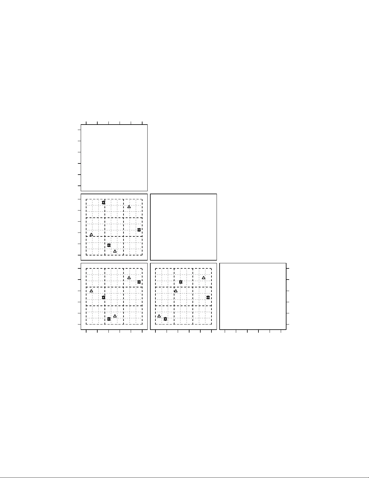
V alidating Sample Av erage Appro ximation Solutions with Negativ ely Dep enden t Batc hes Jia jie Chen Dep ar tment of St a tistics, University of Wisconsin-Madison chen@stat.wisc.edu Cong Han Lim Dep ar tment of Computer Science, University of Wisconsin-Madison conghan@cs.wisc.edu P eter Z. G. Qian Dep ar tment of St a tistics, University of Wisconsin-Madison peterq@stat.wisc.edu Jeff Linderoth ∗ Dep ar tment of Industrial and Systems Engineering, University of Wisconsin-Madison linderoth@wisc.edu Stephen J. W righ t ∗ Dep ar tment of Computer Science, University of Wisconsin-Madison swright@cs.wisc.edu Jan uary 14, 2020 Abstract Sample-a verage approximations (SAA) are a practical means of finding approximate solutions of sto c hastic programming problems in volving an extremely large (or infinite) n umber of scenarios. SAA can also b e used to find estimates of a low er b ound on the optimal ob jectiv e v alue of the true problem whic h, when coupled with an upp er b ound, provides confidence interv als for the true optimal ob jec- tiv e v alue and v aluable information ab out the quality of the approximate solutions. Sp ecifically , the lo wer b ound can b e estimated b y solving multiple SAA problems (each obtained using a particular sampling metho d) and av eraging the obtained ob jectiv e v alues. State-of-the-art metho ds for low er- b ound estimation generate batches of scenarios for the SAA problems indep enden tly . In this paper, w e describe sampling methods that pro duce negatively dependent batc hes, thus reducing the v ariance of the sample-a veraged low er b ound estimator and increasing its usefulness in defining a confidence ∗ W ork is partially supported through a contract from Argonne, a U.S. Department of Energy Office of Science lab oratory . This w ork was supp orted by the Applied Mathematics activity , Adv ance Scien tific Computing Researc h program within the DOE Office of Science 1 in terv al for the optimal ob jectiv e v alue. W e provide conditions under which the new sampling metho ds can reduce the v ariance of the low er b ound estimator, and present computational results to verify that our scheme can reduce the v ariance significan tly , b y comparison with the traditional Latin hypercub e approac h. 1 In tro duction Sto c hastic programming provides a means for formulating and solving optimization problems that contain uncertain ty in the mo del. When the n umber of p ossible scenarios for the uncertain ty is extremely large or infinite, sample-av erage approximation (SAA) provides a means for finding approximate solutions for a reasonable exp enditure of computational effort. In SAA, a finite n umber of scenarios is sampled randomly from the full set of p ossible scenarios, and an appro ximation to the full problem of reasonable size is form ulated from the sampled scenarios and solv ed using standard algorithms for deterministic optimization (suc h as linear programming solvers). Solutions obtained from SAA pro cedures are typically sub optimal. Substan tial researc h has b een done in assessing the quality of an obtained solution (or a set of candidate solutions), and in understanding how differen t sampling metho ds affect the quality of the approximate solution. Imp ortan t information ab out a stochastic optimization problem is pro vided by the optimality gap (Mak et al. 1999, Bayraksan and Morton 2006), whic h pro vides a b ound on the difference b et ween the ob jectiv e v alue for the computed SAA solution and the true optimal ob jective v alue. An estimate of the optimality gap can be computed using upper and low er b ounds on the true optimal ob jective v alue. Mak et al. (1999) prov es that the expected ob jective v alue of an SAA problem is a low er b ound of the ob jective of the true solution, and that this exp ected v alue approac hes the true optimal ob jective v alue as the num b er of scenarios increases. W e can estimate this low er b ound (together with confidence interv als) by solving m ultiple SAA problems, a task that can b e implemented in parallel in an ob vious w ay . An upper b ound can b e computed by taking a candidate solution x and ev aluating the ob jective by sampling from the scenario set, typically taking a larger n umber of samples than were used to set up the SAA optimization problem for computing x . Muc h w ork has b een done to understand the qualit y of SAA solutions obtained from Monte Carlo (MC) sampling, Latin hypercub e (LH) sampling (McKay et al. 1979), and other metho ds. MC generates indep enden t identically distributed scenarios where the v alue of eac h v ariable is pick ed indep enden tly from its corresp onding distribution. The simplicity of this metho d has made it an imp ortan t practical to ol; it has been the sub ject of muc h theoretical and empirical research. Man y results ab out the asymptotic b eha vior of optimal solutions and v alues of MC hav e been obtained; see (Shapiro et al. 2009, Chapter 5) for a review. By con trast with MC, LH stratifies eac h dimension of the sample space in such a w ay that eac h strata has the same probability , then samples the scenarios so that eac h strata is represented in the scenario sample set. This pro cedure in tro duces a dependence b et ween the different scenarios of an individual SAA problem. The sample space is in some sense “uniformly” cov ered on a p er-v ariable basis, thus ensuring that there are no large unsampled regions and leading to impro ved p erformance. Linderoth et al. (2006) provides empirical results showing that the bias and v ariance of a lo wer b ound obtained b y solving multiple SAA problems constructed with LH sampling is considerably smaller than the statistics obtained from an MC-based pro cedure. Theoretical results ab out the asymptotic behavior of these estimates were provided later b y Homem-de Mello (2008). Other results on the p erformance of LH hav e b een obtained, including results on large deviations (Drew and Homem-de Mello 2005), rate of con vergence to optimal v alues (Homem-de Mello 2008), and bias reduction of appro ximate optimal v alues (F reimer et al. 2012), all of which demonstrate the sup eriorit y of LH o ver MC. This fa vorable empirical and theoretical evidence makes LH the current state-of-the-art metho d for obtaining high-quality lo wer b ounds and optimalit y gaps via SAA. In this pap er, we build on the ideas b ehind the LH metho d to obtain 2 LH v ariants with even b etter v ariance prop erties. In the past, when solving a set of SAA problems to obtain a low er-b ound estimate of the true optimal ob jective v alue, eac h batc h of scenarios determining eac h SAA was chosen indep enden tly of the other batc hes. In this pap er, we introduce t wo approaches to sampling — slic e d L atin hyp er cub e (SLH) sampling and slic e d ortho gonal-arr ay L atin hyp er cub e (SOLH) sampling — that yield b etter estimates of the low er b ound by imp osing negative dep endencies b et ween the batc hes in the differen t SAA appro ximations. These approac hes not only stratify within eac h batc h (as in LH) but also b etwe en al l b atches . The SLH approach is easy to implement, while the SOLH approac h provides better v ariance reduction. With these metho ds, w e can significantly reduce the v ariance of the low er b ound estimator even if the size of each SAA problem or the num b er of SAA problems were k ept the same, which can b e especially useful when solving each SAA problem is time consuming or when computing resources are limited. W e will provide theoretical results analyzing the v ariance reduction prop erties of b oth approaches, and present empirical results demonstrating their efficacy across a v ariety of sto c hastic programs studied in the literature. Sliced Latin hypercub e sampling w as introduced first in Qian (2012) and has prov en to b e useful for the collectiv e ev aluation of computer models and ensembles of computer mo dels. Here w e briefly outline the rest of our paper. The next section b egins with a brief description of ho w the optimalit y gap can b e estimated ( § 2.1), a review of Latin h yp ercube sampling ( § 2.2) and an introduction of functional analysis of v ariance ( § 2.3). Section 3 fo cuses on sliced Latin hypercub e sampling. It outlines the construction of dep enden t batches ( § 3.1), describes theoretical results of v ariance reduction based on a certain monotonicity condition ( § 3.2), applies the results to t wo-stage sto c hastic linear program ( § 3.3), and finally studies the relation b et ween the low er b ound estimation and numerical integration ( § 3.4). Section 4 reviews orthogonal arra ys and introduces a metho d to incorp orate these arrays in to the sliced Latin hypercub e sampling, whic h leads to stronger b et ween-batc h negative dep endence. The next tw o sections deal with our computational exp erimen ts. Section 5 describ es the setup and some of the implemen tation details, while Section 6 describ es and analyzes the performance of the new sampling metho ds in the low er bound estimation problem. W e end the pap er in Section 7 with a summary of our results and a discussion of p ossible future research. 2 Preliminaries 2.1 Sto c hastic Programs and Lo wer Bound Estimators W e consider a sto c hastic program of the form min x ∈ X g ( x ) := E [ G ( x, ξ )] , (1) where X ⊂ R p is a compact feasible set, x ∈ X is a v ector of decision v ariables, ξ = ( ξ 1 , ξ 2 , . . . , ξ m ) is a v ector of random v ariables, and G : R p × R m → R is a real-v alued measurable function. Unless stated otherwise, we assume that ξ is a random v ector with uniform distribution on (0 , 1] m and that E is the exp ectation with resp ect to the distribution of ξ . If ξ has a differen t distribution on R m , we can transform it into a uniform random vector on (0 , 1] m as long as ξ 1 , ξ 2 , . . . , ξ m are either (i) indep enden t discrete or con tinuous random v ariables or (ii) dependent random v ariables whic h are absolutely con tinuous (Rosen blatt 1953). Problem (1) may b e extremely challenging to solve directly , since the ev aluation of g ( x ) inv olves a high-dimensional in tegration. W e can replace (1) with the following approximation: min x ∈ X ˆ g n ( x ) := 1 n n X i =1 G ( x, ξ i ) , (2) 3 where ξ 1 , ξ 2 , . . . , ξ n are scenarios sampled from the uniform distribution on (0 , 1] m . The function ˆ g n is called a sample-aver age appr oximation (SAA) to the ob jective g in (1). In this paper w e will frequen tly use the term SAA pr oblem to refer to equation (2). W e use x ∗ and v ∗ to denote a solution and the optimal v alue of the true problem (1), resp ectiv ely , while x ∗ n and v ∗ n denote the solution and optimal v alue of the SAA problem (2), resp ectiv ely . W e introduce here some items of terminology that are used throughout the remainder of the pap er. Let D denote an n × m matrix with ξ T i in (2) as its i th row. Hence, D represents a batch of scenarios that define an SAA problem. W e will refer ξ i to as the i th scenario in D . W e use D (: , k ) to denote the k th column of D , and ξ ik to denote the ( i, k ) entry of D , that is, the k th entry in the i th scenario in D . W e can express the dep endence of v ∗ n in (2) on D explicitly by writing this quantit y as v n ( D ), where v n : (0 , 1] n × m → R . Giv en a distribution o ver the D matrices where ξ 1 , ξ 2 , . . . , ξ n are eac h drawn from the uniform (0 , 1] m distribution but not necessarily indep enden tly , it is w ell known and easy to sho w that the exp ectation with resp ect to the D matrices E [ v n ( D )] ≤ v ∗ giving us a lo wer b ound of the true optimal v alue (Norkin et al. 1998, Mak et al. 1999). E [ v n ( D )] can b e estimated as follows. Generate t indep enden t batc hes D 1 , D 2 , . . . , D t and compute the optimal v alue min v n ( D r ) by solving subpr oblem (2) for each D r , r = 1 , 2 , . . . , t . F rom Mak et al. (1999), a lo wer b ound estimate of v ∗ is L n,t := v n ( D 1 ) + v 2 ( D 2 ) + · · · + v n ( D t ) t . (3) 2.2 Latin Hyp ercub e Sampling Latin hypercub e sampling, whic h stratifies sample p oin ts along each dimension (McKay et al. 1979), has b een used in n umerical integration for man y years. It has been shown that the v ariance of the mean output of a computer experiment under Latin hypercub e sampling can b e muc h low er than for experiments based on Mon te Carlo methods (McKay et al. 1979, Stein 1987, Loh 1996). Let v M C n ( D ) and v LH n ( D ) denote the approximate optimal v alue when the ξ i in D are generated using Mon te Carlo and Latin hypercub e sampling, resp ectiv ely . Homem-de Mello (2008) show ed that the asymptotic v ariance of v LH n ( D ) is smaller than the v ariance of v M C n ( D ) under some fairly general conditions. Extensive n umerical simulations ha ve pro vided empirical demonstrations of the sup eriorit y of Latin hypercub e sampling (Homem-de Mello 2008, Linderoth et al. 2006). T o define Latin hypercub e sampling, w e start with some useful notation. Giv en an integer p ≥ 1, w e define Z p := { 1 , 2 , . . . , p } . Giv en an integer a , the notation Z p ⊕ a denotes the set { a + 1 , a + 2 , . . . , a + p } . F or a real num b er y , d y e denotes the smallest integer no less than y . A “uniform p erm utation on a set of p in tegers” is obtained b y randomly taking a p erm utation on the set, with all p ! p erm utations b eing equally probable. W e hav e the following definition. Definition An n × m array A is a L atin hyp er cub e if eac h column of A is a uniform permutation on Z n . Moreo ver, A is an or dinary L atin hyp er cub e if all its columns are generated indep enden tly . Using an ordinary Latin hypercub e A , an n × m matrix D with scenarios ξ 1 , ξ 2 , . . . , ξ n that defines an SAA problem is obtained as follows (McKay et al. 1979): ξ ik = a ik − γ ik n , i = 1 , 2 , . . . , n, k = 1 , 2 , . . . , m, (4) where all γ ik are U [0 , 1) random v ariables, and the quantities a ik and the γ ik are m utually indep enden t. W e refer the matrix D thus constructed as an or dinary L atin hyp er cub e design . W e no w in tro duce a differen t w ay of lo oking at design matrices D ∈ (0 , 1] n × m that will b e useful when w e discuss extensions to sliced Latin h yp ercub e designs in later sections. W e can write a design matrix D as D = ( B − Θ) /n, (5) 4 where B = ( b ik ) n × m , with b ik = d nξ ik e , Θ = ( θ ik ) n × m , with θ ik = b ik − nξ ik . When D is an ordinary Latin hypercub e design, B is an ordinary Latin hypercub e and θ ik corresp onds to γ ik in (4) for all i = 1 , 2 , . . . , n and k = 1 , 2 , . . . , m . By the properties of an ordinary Latin hypercub e design, the entries in Θ are mutually indep enden t, and Θ and B are independent. W e refer B to as the underlying arr ay of D . The low er b ound on v ∗ can b e estimated from (3) by taking t indep endently gener ate d ordinary Latin h yp ercub e designs D 1 , D 2 , . . . , D t (Linderoth et al. 2006). W e denote this sampling sc heme b y ILH and denote the estimator obtained from (3) b y L I LH n,t . T o illustrate the limitations of the ILH sc heme, Figure 1 displays three independent 3 × 3 ordinary Latin hypercub e designs generated under ILH with n = t = m = 3. Scenarios from each three-dimensional design are denoted by the same symbol, and are pro jected onto each of the three biv ariate planes. The dashed lines stratify eac h dimension in to three partitions. F or any design, eac h of the these three interv als will con tain exactly one scenario in eac h dimension. This scheme co vers the space more “uniformly” than three scenarios that are pick ed iden tically and indep enden tly from the uniform distribution, as happ ens in Mon te Carlo sc hemes. How ever, the combination of p oin ts from all three designs do es not cov er the space particularly well, which giv es some cause for concern, since all designs are b eing used in the low er bound estimation. Sp ecifically , when we combine the three designs together (to give nine scenarios in total), it is usually not the case that eac h of the nine equally spaced in terv als of (0,1] con tains exactly one scenario in an y dimension. This shortcoming provides the in tuition b ehind the sliced Latin hypercub e (SLH) design, whic h we will describ e in the subsequent sections. 2.3 F unctional ANO V A Decomp osition In order to understand the asymp ototic prop erties of estimators arising from Latin-Hypercub e based sam- ples, it is necessary to review the functional analysis of v ariance decomp osition (Owen 1994), also kno wn as functional ANO V A . Let D := { 1 , 2 , . . . , m } represen t the axes of (0 , 1] m asso ciated with an input v ector ξ = ( ξ 1 , ξ 2 , . . . , ξ m ) defined in Section 2.1. Let F k denote the uniform distribution for ξ k , with F := Q m k =1 F k . F or u ⊆ D , let ξ u denote a vector consisting of ξ k for k ∈ u . Define f u ( ξ u ) := Z { f ( ξ ) − X v ⊂ u f v ( ξ v ) } dF D− u , (6) where dF D− u = Q k / ∈ u dF k in tegrates out all comp onen ts except for those included in u , and v ⊂ u is a prop er subset of u . Hence, w e hav e that • f ∅ ( ξ ∅ ) = R f ( ξ ) dF is the mean of f ( ξ ); • f { k } ( ξ k ) = R { f ( ξ ) − f ∅ ( ξ ∅ ) } dF D−{ k } is the main effect function for factor k , and • f { k,l } ( ξ k , ξ l ) = R { f ( ξ ) − f { k } ( ξ k ) − f { l } ( ξ l ) − f ∅ ( ξ ∅ ) } dF D−{ k ,l } is the biv ariate interaction function b et w een factors k and l . When the stochastic program (1) has a unique solution x ∗ and some mild conditions are satisfied, one has v M C n ( D ) − v ∗ σ n,M C ( x ∗ ) d − → Normal(0 , 1) , where σ 2 n,M C := n − 1 v ar[ G ( x ∗ , ξ )] (Shapiro 1991). With additional assumptions, Homem-de Mello (2008) sho ws that v LH n ( D ) − v ∗ σ n,LH ( x ∗ ) d − → Normal(0 , 1) , (7) 5 0.0 0.2 0.4 0.6 0.8 1.0 0.0 0.2 0.4 0.6 0.8 1.0 x1 0.0 0.2 0.4 0.6 0.8 1.0 ● ● ● ● ● ● x2 0.0 0.2 0.4 0.6 0.8 1.0 0.0 0.2 0.4 0.6 0.8 1.0 ● ● ● ● ● ● 0.0 0.2 0.4 0.6 0.8 1.0 ● ● ● ● ● ● 0.0 0.2 0.4 0.6 0.8 1.0 0.0 0.2 0.4 0.6 0.8 1.0 x3 Figure 1: Biv ariate pro jections of three indep enden t 3 × 3 ordinary Latin h yp ercube designs. 6 where σ 2 n,LH := n − 1 v ar[ G ( x ∗ , ξ )] − n − 1 P m k =1 v ar[ G { k } ( x ∗ , ξ k )] + o ( n − 1 ) and G { k } ( x ∗ , ξ k ) is the main effect function of G ( x ∗ , ξ ) as defined in (6). 3 Sliced Latin Hypercub e Sampling Instead of generating D 1 , D 2 , . . . , D t indep enden tly for eac h SAA subproblem, we prop ose a new scheme called slic e d L atin hyp er cub e (SLH) sampling that generates a family of correlated designs. An SLH design (Qian 2012) is a nt × m matrix that can be partitioned in to t separate LH designs, represented b y the matrices D r , r = 1 , 2 , . . . , t , eac h ha ving the same properties as ILH, with resp ect to SAA. SLH was originally introduced to aid in the collectiv e ev aluation of computer mo dels, but here w e demonstrate its utilit y in creating m ultiple SAA problems to solv e. Let L S LH n,t denote the lo wer b ound estimator of v ∗ under SLH. Because the individual designs D r , r = 1 , 2 , . . . , t are LH designs, we ha ve that E ( L S LH n,t ) = E ( L I LH n,t ). Consider t wo distinct batches of scenarios D r and D s for an y r , s = 1 , 2 , . . . , t and r 6 = s . W e will show that when v n ( D ) fulfills a certain monotonicit y condition, v n ( D r ) and v n ( D s ) are negatively dependent under SLH. Compared with ILH, SLH introduces b etwe en-b atch negativ e dep endence while keeping the within-b atch structure intact. As a result, w e exp ect a low er-v ariance estimator: v ar( L S LH n,t ) ≤ v ar( L I LH n,t ). 3.1 Construction Algorithm 1 describ es the construction of the matrices D r , r = 1 , 2 , . . . , t for the SLH design. W e use notation D r (: , k ) for the k th column of D r , ξ r,i for the i th scenario of D r , and ξ r,ik for the k th en try in ξ r,i , for i = 1 , 2 , . . . , n , k = 1 , 2 , . . . , m , and r = 1 , 2 , . . . , t . Algorithm 1 Generating a Sliced Latin Hyp ercube Design Step 1. Randomly generate t independent ordinary Latin hypercub es A r = ( a r,ik ) n × m , r = 1 , 2 , . . . , t . Denote the k th column of A r b y A r (: , k ), for k = 1 , . . . , m . Step 2. F or k = 1 , 2 , . . . , m , do the following indep enden tly: Replace all the ` s in A 1 (: , k ) , A 2 (: , k ) , . . . , A t (: , k ) b y a random permutation on Z t ⊕ t ( ` − 1), for ` = 1 , 2 , . . . , n . Step 3. F or r = 1 , 2 , . . . , t , obtain the ( i, k )th entry of D r as follo ws: ξ r,ik = a r,ik − γ r,ik nt , (8) where the γ r,ik are U [0 , 1) random v ariables that are mutually indep enden t of the a r,ik . By v ertically stac king the matrices D 1 , D 2 , . . . , D t , w e obtain the nt × m matrix represen ting the SLH design, as defined in Qian (2012). As in (5), we can express each D r as D r = ( B r − Θ r ) /n, (9) where B r = ( b r,ik ) n × m with b r,ik = d nξ r,ik e and Θ r = ( θ r,ik ) n × m . W e hav e the following prop osition regarding prop erties of the SLH design, including dep endence of the batches. (This result is closely related to (Qian 2012, Lemma 2).) Prop osition 3.1 Consider the SLH design with D r , r = 1 , 2 , . . . , t c onstructe d ac c or ding to Algorithm 1, with B r and Θ r , r = 1 , 2 , . . . , t define d as in (9) . The fol lowing ar e true. 7 (i) B r , r = 1 , 2 , . . . , t ar e indep endent or dinary L atin hyp er cub es. (ii) B r and Θ r ar e indep endent, for e ach r = 1 , 2 , . . . , t . (iii) Within e ach Θ r , r = 1 , 2 , . . . , t , the θ r,ik ar e mutual ly indep endent U [0 , 1) r andom variables. (iv) F or r , s = 1 , 2 , . . . , t with r 6 = s , θ r,ik is dep endent on θ s,ik if and only if B r,ik = B s,ik ; (v) The D r , r = 1 , 2 , . . . , t ar e or dinary L atin hyp er cub e designs, but they ar e not indep endent. Pro of (i) According to (9) and Step 2 in the ab o ve construction, B r is the same as A r in Step 1 prior to the replacement step, and the result follo ws. (ii) Note that b r,ik = l a r,ik − γ r,ik t m =  a r,ik t  where the a r,ik are v alues in A r after the replacement in Step 2 of the construction ab o ve. By (8) and (9), we hav e θ r,ik = b r,ik − a r,ik t + γ r,ik t =  t l a r,ik t m − a r,ik  /t + γ r,ik /t. (10) According to Step 2 of the construction, for each r = 1 , 2 , . . . , t , i = 1 , 2 , . . . , n and k = 1 , 2 , . . . , m , the quantit y t d a r,ik t e − a r,ik is randomly selected among Z t and is independent of B r . Since the γ r,ik are independent of the a r,ik , the claim is prov ed. (iii) F or eac h r = 1 , . . . , t and k = 1 , . . . , m , the quantities { t  a r, 1 k t  − a r, 1 k , t  a r, 2 k t  − a r, 2 k , . . . , t  a r,nk t  − a r,nk } are indep enden tly and randomly selected among n different Z t ’s, respectively . Thus, the θ r,ik are mutually indep enden t within Θ r . In other words, the t d a r,ik t e − a r,ik , i = 1 , 2 , . . . , n are m utually indep enden t discrete uniform random v ariables on Z t , suc h that the θ r,ik are U [0 , 1) random v ariables, b y (10). (iv) It suffices to show that t  a r, 1 k t  − a r, 1 k and t  a r,nk t  − a s,nk are dep enden t if and only if B r,ik = B s,ik . That is true because t  a r, 1 k t  − a r, 1 k and t  a r,nk t  − a s,nk are selected from the same Z t when B r,ik = B s,ik . (v) The result follows directly from (i), (ii), (iv), and the definition of the ordinary Latin h yp ercub e design.  Figure 2 displa ys the biv ariate pro jection of the three 3 × 3 ordinary Latin hypercub e designs, each denoted by a different sym b ol, whic h are generated under an SLH scheme. F or eac h design, each of the three equally spaced interv als of (0 , 1] contains exactly one scenario in each dimension. In contrast to Figure 1, when we com bine the three designs together, each of the nine equally spaced in terv als of (0 , 1] con tains exactly one scenario in an y one dimension. 3.2 Monotonicit y Condition W e derive theoretical results to show v ar( L S LH n,t ) ≤ v ar( L I LH n,t ) under a monotonicity condition that will b e defined shortly . Definition W e sa y that tw o random v ariables Y and Z are ne gatively quadr ant dep endent if P ( Y ≤ y , Z ≤ z ) ≤ P ( Y ≤ y ) P ( Z ≤ z ) , for all y , z . Definition Let B = ( b ik ) denote the underlying ordinary Latin hypercub e of D in (5) suc h that D = ( B − Θ) /n . Let v n ( D ) = H (∆; B ) given B , where H (∆; B ) : (0 , 1] n × m → R and ∆ = ( δ `k ), with δ `k = θ ik suc h that b ik = ` for ` = 1 , 2 , . . . , n and k = 1 , 2 , . . . , m . The function v n ( D ) is said to b e monotonic if the following tw o conditions hold: (a) for all B , H (∆; B ) is monotonic in each argument of ∆, and (b) the direction of the monotonicity in each argument of ∆ is consisten t across all B . 8 0.0 0.2 0.4 0.6 0.8 1.0 0.0 0.2 0.4 0.6 0.8 1.0 x1 0.0 0.2 0.4 0.6 0.8 1.0 ● ● ● ● ● ● x2 0.0 0.2 0.4 0.6 0.8 1.0 0.0 0.2 0.4 0.6 0.8 1.0 ● ● ● ● ● ● 0.0 0.2 0.4 0.6 0.8 1.0 ● ● ● ● ● ● 0.0 0.2 0.4 0.6 0.8 1.0 0.0 0.2 0.4 0.6 0.8 1.0 x3 Figure 2: Biv ariate pro jections of a sliced Latin h yp ercub e design that consists of three 3 × 3 ordinary Latin h yp ercube designs, each denoted by a differen t symbol. 9 Example Consider D = ( ξ ik ) 3 × 2 . Let v n ( D ) = P 3 i =1 P 2 k =1 ( ξ ik − 1 / 3) 2 . When B =   3 1 2 3 1 2   , w e hav e δ 11 = θ 31 , δ 21 = θ 21 , δ 31 = θ 11 , δ 12 = θ 12 , δ 22 = θ 32 , and δ 32 = θ 22 and H (∆; B ) = 1 9  δ 2 11 + (1 − δ 21 ) 2 + (2 − δ 31 ) 2 + δ 2 12 + (1 − δ 22 ) 2 + (2 − δ 32 ) 2  , Th us, H (∆; B ) is increasing in δ 11 and δ 12 while it is decreasing in the other δ ik s, for δ ik ∈ (0 , 1]. This is true for an y underlying ordinary Latin h yp ercube B , since δ 11 and δ 12 are alw ays asso ciated with v alues in D which are b et ween (0,1/3] in this example. By definition, v n ( D ) is monotonic. The monotonicit y condition can b e chec ked by directly studying the function v n ( D ), but it can also b e sho wn to b e satisfied if the stochastic program has certain nice prop erties. Later we will prov e some sufficien t conditions for tw o-stage sto c hastic linear programs and give a simple argumen t to show ho w some problems from the literature hav e the monotonicit y prop ert y . Qian (2012) pro ves that the function v alues of an y tw o scenarios in a sliced Latin h yp ercube design are negatively quadrant dependent. The next lemma extends this result, sho wing the function v alues of an y tw o b atches in a sliced Latin h yp ercub e design are also negatively quadrant dep enden t, under the monotonicit y assumption on v n ( D ). Lemma 3.2 Consider D 1 , D 2 , . . . , D t gener ate d by Algorithm 1. If v n ( D ) is monotonic, then we have E [ v n ( D r ) v n ( D s )] ≤ E [ v n ( D r )] E [ v n ( D s )] , for any r, s = 1 , 2 , . . . , t with r 6 = s . Pro of Giv en t wo ordinary Latin hypercub es B r and B s in (9), let D r = ( B r − Θ r ) /n and D s = ( B s − Θ s ) /n denote tw o slices generated b y (8). Since the underlying Latin h yp ercubes are fixed for D r and D s , the only random parts in the definition are Θ r and Θ s . Define H (∆ r ; B r ) = v n ( D r ) = v n ( B r /n − Θ r /n ) and H (∆ s ; B s ) = v n ( D s ) = v n ( B s /n − Θ s /n ), where ∆ r and ∆ s are n × m matrices with the ( k , ` )th en try defined as δ r,`k = θ r,ik and δ s,`k = θ s,ik suc h that B r,ik = B s,ik = ` for ` = 1 , 2 , . . . , n and k = 1 , 2 , . . . , m . By Proposition 3.1 (iii) and (iv), we can find nm indep enden t pairs of random v ariables: ( δ r , δ s ) for ` = 1 , 2 , . . . , n , k = 1 , 2 , . . . , m . By (Lehmann 1966, Theorem 2), the monotonicity assumption of v n ( D ), and the pro of of (Qian 2012, Theorem 1), we hav e E [ H (∆ r ; B r ) H (∆ s ; B s )] ≤ E [ H (∆ r ; B r )] E [ H (∆ r ; B r )] , whic h is equiv alent to E [ v n ( D r ) v n ( D s ) | B r , B s ] ≤ E [ v n ( D r ) | B r ] E [ v n ( D r ) | B s ] . T aking exp ectations of b oth s ides gives E [ v n ( D r ) v n ( D s )] ≤ E { E [ v n ( D r ) | B r ] } E { E [ v n ( D s ) | B s ] } = E [ v n ( D r )] E [ v n ( D s )] . The last equality holds b ecause B r and B s are independent, by Proposition 3.1 (i).  The next result is an immediate consequence of Lemma 3.2. It indicates that the v ariance of the lo wer-bound estimator could b e reduced by using SLH, when v n ( D ) is monotonic. 10 Theorem 3.3 Consider two lower b ound estimators L I LH n,t and L S LH n,t in (3) obtaind under ILH and SLH, r esp e ctively. Supp ose v n ( D ) in monotonic, then for any n and t , we have that v ar( L S LH n,t ) ≤ v ar( L I LH n,t ) . Ev en if the monotonicit y condition does not hold, we can prov e similar statemen ts about the asymptotic b eha vior of the v ariance of ILH and SLH. Theorem 3.4 gives an asymptotic result that sho ws the same conclusion can b e drawn as in Theorem 3.3 ev en if the monotonicit y condition do es not hold. Theorem 3.4 L et D denote an n × m L atin hyp er cub e design b ase d on a L atin hyp er cub e B such that D = ( B − Θ) /n . L et H (∆; B ) = v n ( D ) . Supp ose E { [ v n ( D )] 2 } is wel l define d. As t → ∞ with n fixe d, the fol lowing ar e true. (i) v ar( L I LH n,t ) = t − 1 v ar[ v n ( D )] . (ii) v ar( L S LH n,t ) = t − 1 v ar[ v n ( D )] − t − 1 P n ` =1 P m k =1 R { E [ H { `k } ( δ `k ; B )] } 2 dδ `k + o ( t − 1 ) , wher e H { `k } ( δ `k ; B ) is the main effe ct function of H (∆; B ) with r esp e ct to δ `k . (iii) If v n ( D ) = P m k =1 v n, { k } ( D (: , k )) is additive, wher e v n, { k } : (0 , 1] n → R , then v ar( L S LH n,t ) = o ( t − 1 ) . Pro of (i) When D 1 , D 2 , . . . , D t are sampled indep enden tly under ILH, cov[ v n ( D r ) , v n ( D s )] = 0 for an y r 6 = s . Thus, we hav e v ar( L I LH n,t ) = t − 1 v ar[ v n ( D )]. (ii) When D 1 , D 2 , . . . , D t are sampled under SLH, we hav e v ar( L S LH n,t ) =v ar " t − 1 t X i =1 v n ( D i ) # = t − 2 t X i =1 v ar [ v n ( D i )] + t − 2 X 1 ≤ r N , for some u ⊆ D and | u | ≥ 3, can inflate the v ariance due to higher-order interactions. This side effect is less significant if the biv ariate in teractions dominate higher order in teractions, which is true in most problems. In addition, w e need to emphasize that each batch under SOLH is based on an OA( n, m, t, 1), which is a Latin hypercub e design instead of an ordinary Latin hypercub e. W e conjecture that Assumption 3.1 still holds in this case, and the biv ariate v ariance reduction is due to the b et ween-batc h negative dep endence rather than the within-batch non-ordinary Latin h yp ercub e structure. This conjecture is consistent with our computational observ ations, as shown b elo w. 4.4 Practical Considerations Using the SOLH method is not just a matter of pic king the desired n, m v alues of the dimensions of the design matrices and the n umber of batc hes t , like it was in the SLH case. Picking the appropriate orthogonal arra y requires some understanding of the tradeoffs b et ween the different choices. Consider an O A( n 2 , m + 1 , n, 2). The b enefits of using these arrays include (i) each batch is based on an ordinary Latin hypercub e, and (ii) there is no coincidence defect. Ho wev er, w e hav e to solve n batc hes of n scenarios eac h. W e wan t n to be large enough to ensure that the quan tity x ∗ n con verges and that the bias v ∗ − E [ v n ( D )] is small, but solving n batches could b e computationally infeasible. One w ay around this computational hurdle is to relax the restriction that w e use all the batc hes that are generated b y the SOLH metho d. W e can use just the first t batches, and we will call this the sliced partial orthogonal-ara y-based Latin hypercub e metho d (SPOLH). Let υ denote the fraction of the num b er of batc hes generated by SOLH. SPOLH can p erform b etter than SLH since υ of the v ariance due to biv ariate in teractions can b e remov ed. How ever, when υ is small (10%, say), it do es not guarantee substantial v ariance reduction from SLH to SPOLH. W e can alternatively use orthogonal arra ys with a higher index v alue (i.e. λ > 1) allowing us to hav e a t that is m uch smaller than n . In this case, there is coincidence defect and picking and generating the righ t orthogonal arrays with desirable n, m, t v alues with lo w M ( u, r ) can b e difficult. 5 Exp erimen tal Setup T o illustrate the effectiv eness of negativ ely dependent designs for estimation of the lo wer bound on the ob jective v alue in sto c hastic programs, we p erform computational exp erimen ts using data sets from the literature. This section pro vides some details on our implementations and test problems. 5.1 Implemen tation W e estimate a single lo wer b ound b y choosing a design family , obtaining a set of sampled approximations using this design family , and finally solving these approximations. The p erformance of a sampling scheme is assessed by rep eating this pro cess to obtain a n umber of low er b ound estimates. W e then calculate the mean and v ariance of these estimates. W e augmen ted the SUTIL library (Czyzyk et al. 2000), a C and C++ based library for manipulating sto c hastic programming instances with a design-based sampling framework. This augmen ted SUTIL library can tak e an orthogonal array as input and generate an orthogonal-arra y-based design family as output. The library can generate other design families from scratch. W e used a C library due to Owen (a v ailable 21 at http://lib.stat.cmu.edu/ ) to generate the orthogonal arrays. The SUTIL softw are produces the extensiv e form (or deterministic equiv alent) linear program of eac h sampled instance and outputs the linear program as an MPS file. These files are fed into the commercial linear programming solv er Cplex v12.5 and solved using the barrier metho d. All the timed exp erimen ts were run on an In tel Xeon X5650 (24 cores @ 2.66Ghz) serv er with 128GB of RAM, and 16 of the 24 cores a v ailable on the mac hine were used. Other exp erimen ts w ere run on the HTCondor grid (Thain et al. 2005) of the Computer Sciences departmen t at Univ ersity of Wisc onsin-Madison. They required more than a w eek of wall-clock time to complete. 5.2 T est Problems Our five test problems were drawn from the sto c hastic programming literature. In fact, they are the same problems that were studied in Linderoth et al. (2006). These problems are sp ecified in SMPS file format (a sto c hastic-programming extension of MPS), and hav e finite discrete distributions for their random v ariables. 20term , first describ ed in Mak et al. (1999), is a model of a motor freight carrier’s op erations. The first stage v ariables represent p ositions of a fleet of vehicles at the b eginning of a day . The second- stage v ariables determine the mo vemen ts of the fleet through a net work to satisfy point-to-point demands for shipments (with p enalties for unsatisfied demands), and to end the da y with the fleet bac k in their initial positions. gbd is deriv ed from an aircraft allo cation problem originally describ ed in the textb ook of Dantzig (1963, Chapter 28). F our differen t types of aircraft are to be allo cated to routes to maximize the profit under uncertain demand for each route. There are cos ts asso ciated with using eac h aircraft t yp e, and when the capacity do es not meet demand. LandS is a mo dification by Linderoth et al. (2006) of a simple problem in electrical inv estment planning describ ed by Louv eaux and Smeers (1988). The first-stage v ariables represent capacities of different new technologies, and the second-stage v ariables represent pro duction of each of the differen t modes of electricit y from eac h of the tec hnologies. ssn (Sen et al. 1994) is a problem from telecommunications netw ork design. The owner of a netw ork sells priv ate-line services betw een pairs of nodes in the net work. During the first stage of the problem, the o wner has a budget for adding bandwidth (capacit y) to the edges in the net work. In the second stage, to satisfy uncertain demands for service betw een eac h pair of no des, short routes b et ween t wo no des with sufficien t total bandwidth must b e iden tified. Unmet demands incur costs, and the goal of the problem is to minimize the expected costs. storm is a cargo flight scheduling problem describ ed by Mulvey and Ruszczy ´ nski (1993). The goal is to schedule cargo-carrying flights ov er a set of routes in a netw ork, where the amount of cargo deliv ered to each no de is uncertain. In the first stage, the n umber of planes of each type on each route is decided. In the second stage, the random v ariables are the demands on the amounts of cargo to b e deliv ered b etw een nodes. The goal is to minimize (1) the costs that comes from assigning the planes and balancing payloads, and (2) the p enalties asso ciated with unmet demands. All of these problems fit our monotonicity assumption defined in § 3.2. The intuition for this prop erty is straightforw ard – the ob jective in eac h problem is to minimize costs and p enalties that come from unmet demands. Hence, as the demand increases, the ob jective v alue alw ays increases. W e outline some facts ab out the random v ariables and optimal solution for each problem in T able 4. The random v ariables for all the problems are independent from each other. F or the distribution column, w e use ‘uniform’ to refer to a uniform distribution o ver all p ossible v alues, and ‘irregular’ for an y other distribution. 22 Additionally , we note that the distribution of eac h of the random v ariables of LandS appro ximate a linear function as it has a uniform distribution ov er evenly spaced p oin ts. The upp er- and low er-b ound estimates (with 95% confidence in terv als) are obtained from (Linderoth et al. 2006, T able 4) with n = 5000. W e will refer to the quantities in this table in our discussion of the computational results. T able 4: Prop erties of our sto c hastic programming test problems Random V ariables Bounds (95% confidence interv al) Num b er Possible V alues Distribution Lo wer Upp er 20term 40 2 Uniform 254298 . 57 ± 38 . 74 254311 . 55 ± 5 . 56 gb d 5 13 - 17 Irregular 1655 . 62 ± 0 . 00 1655 . 628 ± 0 . 00 LandS 3 100 Uniform 225 . 62 ± 0 . 02 225 . 624 ± 0 . 005 ssn 86 4 - 7 Irregular 9 . 84 ± 0 . 10 9 . 913 ± 0 . 022 storm 117 5 Uniform 15498657 . 8 ± 73 . 9 15498739 . 41 ± 19 . 11 6 Computational Results In this section w e will summarize the computational results and observ ations. F or each com bination of sampling scheme, n umber of scenarios, and n umber of batches, we p erform the lo wer bound estimation pro cess 100 times, and compute the mean and standard error of the 100 low er bounds obtained. Before we pro ceed with our observ ations, we should e mphasize that while we use the same problems as in Linderoth et al. (2006), our results are not directly comparable. In particular, Linderoth et al. (2006) fo cus on results based on analysis of the ob jective v alues across 10 uncorrelated subproblems of a single replicate (or similarly , across 10 replicates of one subproblem eac h). W e fo cus on the analysis of the mean SAA ob jective v alues b et ween man y (p otentially correlated) subproblems across 100 replicates. Hence, the results in Linderoth et al. (2006) yield a measure of the quality of a single low er-b ound estimate, while our results compare the quality of several different low er b ound estimates. All data used in this analysis — sp ecifically , the ob jective v alues obtained by solving each LP corre- sp onding to eac h batch — can b e obtained at the web site for this pap er at http://pages.cs.wisc.edu/ ~ conghan/slhd/ . 6.1 Timing Information T able 5 shows the wall-clock time required to solve a single sampled approximation for the fiv e test problems using our timing setup as describ ed in § 5.1. Ev en though the time to generate a batch of scenarios increases as the sampling metho d increases in complexit y , this time is insignificant compared to the rest of the pro cess and hence was not included in this table. The timings were obtained for each problem and num b er of scenarios by a veraging across 16 subproblems constructed from all design metho ds w e considered. The timing increases with the num b er of scenarios at a sup erlinear rate. Hence, when the underlying problem is difficult and the num b er of scenarios is sufficiently high, solving many batc hes could b e extremely time consuming ev en with m ultiple machines. 6.2 Mean and Standard Error of the Different Sampling Metho ds In our first set of exp erimen ts, we computed the means and standard errors of the lo wer bound estimates of the ob jective v alue ov er 100 replicates of eac h sampling metho d and each num b er of scenarios. W e fixed the n umber of subproblems at t = 16, while v arying the num b er of scenarios per batch according to n ∈ { 128 , 256 , 512 , 1024 } . W e tested four differen t sampling metho ds: Monte Carlo (MC), indep enden t ordinary Latin h yp ercube (ILH), Sliced Latin hypercub e (SLH) and Sliced Partial Orthogonal Array Based 23 T able 5: W all clo c k times (in seconds) for solving one sample appro ximation problem with v arying num b ers of scenarios no. of scenarios 256 512 1024 20term 4.83 11.12 30.09 gb d 0.03 0.10 0.17 LandS 0.07 0.12 0.25 ssn 10.36 23.80 61.63 storm 16.40 37.85 84.22 Latin hypercub e based on Bush orthogonal arra ys (BUSH), which are O A ( n 2 , m + 1 , n, 2). Since we are only using 16 out of n possible batches, we are discarding muc h of the orthogonal arra y , and therefore not ac hieving m uch tw o-dimensional stratification in our negativ ely dependent designs. Computational results are summarized in T able 6. T able 6: Mean and v ariance of estimates of the low er b ound with 16 batches, ov er 100 replicates. 128 scenarios 256 scenarios 512 scenarios 1024 scenarios Mean SE Mean SE Mean SE Mean SE 20term MC 254253.1 244.1 254292.1 160.2 254297.4 95.1 254311.3 69.3 ILH 254296.7 58.2 254311.1 39.8 254306.4 25.6 254311.0 19.9 SLH 254285.9 53.3 254303.0 45.0 254307.6 31.5 254310.0 23.8 BUSH 254296.0 54.8 254299.2 38.3 254307.5 30.2 254312.8 22.1 gb d MC 1653.207 14.292 1654.061 10.540 1655.124 6.881 1656.837 5.585 ILH 1655.637 1.094 1655.760 0.670 1655.606 0.260 1655.616 0.157 SLH 1655.640 0.281 1655.622 0.171 1655.615 0.066 1655.635 0.044 BUSH 1655.602 0.275 1655.609 0.167 1655.645 0.080 1655.632 0.043 LandS MC 225.3951 1.2923 225.7044 0.9876 225.5539 0.6106 225.6881 0.4622 ILH 225.6314 0.0549 225.6233 0.0332 225.6249 0.0278 225.6301 0.0158 SLH 225.6135 0.0471 225.6248 0.0370 225.6259 0.0255 225.6295 0.0177 BUSH 225.6159 0.0522 225.6191 0.0319 225.6274 0.0266 225.6295 0.0185 ssn MC 7.426 0.387 8.403 0.287 9.028 0.188 9.411 0.142 ILH 8.945 0.267 9.378 0.186 9.635 0.150 9.770 0.103 SLH 8.877 0.225 9.321 0.203 9.609 0.137 9.775 0.087 BUSH 8.929 0.258 9.374 0.181 9.656 0.134 9.785 0.091 storm MC 15498662.4 7441.1 15498518.5 5517.1 15498532.9 3648.5 15498473.7 2838.3 ILH 15498741.0 454.9 15498678.8 257.0 15498698.9 151.2 15498716.6 98.2 SLH 15498690.0 245.2 15498683.9 159.0 15498695.4 104.6 15498721.5 79.3 BUSH 15498699.6 238.7 15498731.9 149.6 15498688.7 115.6 15498709.3 85.4 W e b egin with some general observ ations ab out the mean of the low er bound estimates. As observ ed in other experiments (Linderoth et al. 2006, F reimer et al. 2012), the Mon te Carlo metho d is significantly w orse than Latin Hyp ercub e-based metho ds in terms of the bias. As exp ected, the Latin Hyp ercub e-based metho ds pro duce statistically-indistinguishable low er b ounds. By comparing with the results of T able 4, for all problems except ssn , ILH attains a mean extremely close to the true mean when the num b er of scenarios is 1024, and is already very close with a smaller n umber of scenarios. ssn is known to b e a c hallenging problem, requiring at least 512 scenarios to attain a reasonable estimate of the optimum even for the three Latin hypercub e schemes. Increasing the num b er of scenarios b ey ond 1024 would con tinue to improv e the quality of the estimates. Linderoth et al. (2006) pro vide a more detailed description of the b eha vior of SAA for the ssn problem. 24 W e now turn to the standard error. By this measure, for every problem except ssn , w e see that MC p erforms m uch w orse than the other metho ds. It is only slightly w orse for ssn . This table shows situations in which the negatively dependent designs of SLH and BUSH b egin to distinguish themselves from ILH. F or gbd and storm , we can see large improv ements from ILH to SLH/BUSH. The improv ement from ILH to SLH/BUSH is muc h less pronounced in ssn , b eing in general smaller than the improv ement from MC to ILH, and in one case performing sligh tly worse than ILH. How ever, w e should note that in all the problems, BUSH and SLH ha ve roughly similar performance. This observ ation suggests that when we use to o few subproblems, the effect of partial orthogonality on p erformance is not significan t. F or 20term and LandS , the Latin hypercub e schemes ILH, SLH, and BUSH p erform similarly . In the case of 20term , this similarity is unsurprising. The b enefits of SLH ov er ILH come from the increased stratification that comes from the sliced structure, but since each v ariable can only tak e on tw o v alues, eac h with probability 0 . 5, any stratification that divides the probability space into a multiple of tw o would p erform equally well. In the case of LandS , w e susp ect that the similarit y of p erformance is due to the smo othness of the distribution of the random v ariables. In fact, the cum ulative distribution function is essen tially linear. W e ha ve found that when w e mo dify the distribution to b e more irregular or to to b e a uniform distribution ov er a muc h smaller set, it tends to driv e up the standard error and to cause SLH to ha ve a significantly smaller standard error than ILH. W e now consider a greater n umber of subproblems for each n and new alternativ es for the underlying orthogonal arra ys. In addition to the four different sampling metho ds considered earlier, w e show tw o additional v ariants: Sliced Orthogonal Ar ray Based Latin hypercub e based on Bose-Bush ort hogonal arra ys (BB), and indep endent batches taken ov er several BB (INDBB). Bose-Bush orthogonal arrays hav e an O A( λs 2 , m + 1 , s, 2) structure. W e pick s to b e equal to the n umber of subproblems, and define λ = n/s . With these c hoices, the sliced designs achiev e full tw o-dimensional stratification, making BB an example of SOLH sampling. W e include INDBB in our exp erimen ts to help isolate the factors that lead to the stronger p erformance of BB. If each slice of the BB design has some sp ecial structure that leads to impro ved p erformance, then INDBB designs should p erform b etter than ILH, and the p erformance of INDBB should b e close to that of BB. Ho wev er, if the performance gains of BB are primarily due to the better tw o-dimensional stratification, then w e would exp ect INDBB to perform no b etter than ILH. The numerical results support the second claim. Results a re shown in T able 7. Many of the observ ations ab out MC/ILH/SLH/BUSH from T able 6 carry ov er. Also, comparing the standard error of MC/ILH/SLH/BUSH b et w een the tw o tables, we notice a factor of √ 2 or 2 difference in standard error, dep ending on whether the num b er of subproblems w as doubled or quadrupled. This factor is consisten t with Theorem 3.4. The lo wer bound estimates are roughly the same in b oth tables, demonstrating that changing the num b er of subproblems do es not affect the bias. T able 7 shows a considerable adv antage for BB ov er ILH. In fact, B B is b etter than all other metho ds tested, except on gbd , where it performs similarly to SLH/BUSH. On LandS , BB p erforms about 5-10 × b etter than the other sliced sampling metho ds. A p ossible explanation for this h uge impro vemen t is that the total num b er of random v ariables is just three, so ha ving tw o-dimensional stratification would cov er a large p ortion of the p ossible in teractions b etw een v ariables. In the case of ssn , the impro vemen t from ILH to BB is comparable to the impro vemen t from MC to ILH, a bigger factor than is observed for any other problem. Finally , we turn our atten tion to running times. The standard error of the estimates b et w een the results for 512 scenarios and 16 slices in T able 6 and 256 scenarios and 32 slices in T able 7 are similar. Since the timing scales sup erlinearly in the num b er of scenarios ( § 6.1), the amount of time it takes to solve ct sampled appro ximations of n scenarios sequentially can b e substantially less than solving t sampled appro ximations of cn . Each batch could also b e solved independently and in parallel. This suggests that if computing resources on each machine is limited and using SLH/SPOLH with cn scenarios and t batc hes 25 T able 7: Mean and standard error of estimates of the lo wer b ound with 32 or 64 batches (o ver 100 replicates) (scenarios, batches) (128,32) (256,32) (512,64) (1024,64) Mean SE Mean SE Mean SE Mean SE 20term MC 254295.4 164.5 254305.0 116.3 254301.1 54.4 254313.4 36.9 ILH 254305.7 43.4 254296.4 29.2 254307.0 16.8 254309.1 9.9 SLH 254294.2 45.8 254306.3 28.5 254306.2 14.3 254308.5 11.3 BUSH 254293.7 36.5 254305.3 27.8 254306.7 13.6 254309.4 10.1 BB 254296.1 20.9 254305.3 18.9 254307.3 7.6 254310.3 4.9 INDBB 254294.4 39.3 254301.1 29.9 254308.3 15.2 254309.1 11.1 gb d MC 1653.130 9.485 1654.699 7.091 1655.488 3.389 1655.655 2.986 ILH 1655.550 0.849 1655.658 0.390 1655.633 0.164 1655.628 0.094 SLH 1655.649 0.169 1655.620 0.066 1655.628 0.017 1655.628 0.011 BUSH 1655.628 0.163 1655.628 0.066 1655.629 0.017 1655.628 0.011 BB 1655.614 0.170 1655.626 0.072 1655.629 0.018 1655.627 0.011 INDBB 1655.618 0.799 1655.582 0.483 1655.618 0.140 1655.641 0.096 LandS MC 225.6448 0.9108 225.6300 0.6092 225.6431 0.2844 225.5845 0.2202 ILH 225.6151 0.0344 225.6190 0.0248 225.6255 0.0131 225.6298 0.0088 SLH 225.6172 0.0351 225.6260 0.0263 225.6253 0.0124 225.6287 0.0087 BUSH 225.6155 0.0332 225.6247 0.0225 225.6260 0.0116 225.6269 0.0081 BB 225.6178 0.0068 225.6247 0.0047 225.6270 0.0015 225.6282 0.0010 INDBB 225.6202 0.0370 225.6220 0.0252 225.6258 0.0123 225.6281 0.0085 ssn MC 7.426 0.275 8.412 0.197 9.011 0.094 9.389 0.071 ILH 8.908 0.184 9.378 0.127 9.628 0.073 9.767 0.045 SLH 8.911 0.198 9.386 0.131 9.614 0.064 9.771 0.054 BUSH 8.905 0.175 9.390 0.123 9.634 0.064 9.770 0.051 BB 8.925 0.105 9.408 0.083 9.627 0.029 9.767 0.022 INDBB 8.938 0.185 9.381 0.134 9.620 0.078 9.763 0.049 storm MC 15499036.3 5185.4 15498564.6 3653.0 15498659.9 2039.3 15498513.0 1263.0 ILH 15498674.5 377.4 15498717.2 179.3 15498690.9 68.6 15498715.7 43.3 SLH 15498658.3 149.0 15498712.7 99.8 15498699.4 53.4 15498718.1 37.0 BUSH 15498687.3 133.0 15498707.0 104.1 15498701.9 47.0 15498721.9 38.4 BB 15498686.1 76.1 15498710.4 42.5 15498693.4 22.0 15498720.7 12.6 INDBB 15498674.6 297.4 15498712.5 201.2 15498695.8 67.9 15498720.7 43.1 26 is computationally infeasible, using SOLH with with n scenarios and ct batc hes can b e an effective w ay of reducing the standard error. W e conclude that for a fairly small num b er of s ubproblems, the sliced sampling metho ds p erform at least as well as Latin hypercub e sampling, and in fact sho w significant impro vemen t in some cases. Once w e increase the num b er of subproblems and exploit the full “orthogonality” prop erty of the orthogonal arra ys, w e see a substantial improv ement in al l cases. Thus, if the computational budget will only allow a small num b er of batches for the giv en v alue of n for which a low er b ound v n is b eing estimated, there is significan t computational b enefit to using the more sophisticated sampling metho ds in tro duced in this w ork. 7 Conclusions and F uture W ork In this pap er, we prop ose the use of tw o types of negatively dep enden t designs to improv e the low er b ound of the ob jective v alue. Sliced Latin hypercub e sampling is easy to implement since SLH does not imp ose an y restriction on the num b er of batc hes t and the num b er of scenarios in each batch. W e introduce the concept of monotonicity for tw o-stage sto c hastic linear programs, and w e provide a non-asymptotic result sho wing that SLH can be b etter than ILH for problems with this monotonicit y prop ert y . On the other hand, we sho w that SLH is asymptotically equiv alent to ILH if the distribution of the random vector has finite supp ort and the approximate solutions conv erge. Our computational results supp orts the theory , sho wing that SLH p erforms no worse than ILH and in some cases p erforms significantly b etter than ILH. T o improv e upon SLH, we consider sliced orthogonal array-based Latin hypercub e sampling schemes, whic h achiev e stronger negativ e dep endence b et ween batc hes. The c hoice of the underlying orthogonal arra y can make a h uge difference in v ariance reduction. W e provide empirical results showing that when w e are able to exploit the full orthogonalit y of the underlying orthogonal arra y , using Bose-Bush orthogonal arra ys (Bose and Bush 1952), the p erformance is significan tly b etter than when we use only part of an orthogonal arra y . Our work treats Latin h yp ercube sampling as the baseline metho d, in part because it was in vesti- gated in earlier w ork (Linderoth et al. 2006). Other sampling metho ds, such as U sampling (T ang 1993, T ang and Qian 2010) and randomized quasi-Monte Carlo (Niederreiter 1992, Owen 1995, Homem-de Mello 2008) could ha ve b een used instead for constructing a single SAA problem. W e can carry o ver the idea of negativ ely dep endent designs to these adv anced within-batch sampling techniques. F or U sampling, a strength-t wo orthogonal array-based Latin hypercub e design could b e generated for eac h SAA problem. The t underlying strength-t wo orthogonal arrays can be obtained by slicing a larger strength-three or- thogonal arra y . F or randomized quasi-Monte Carlo, w e can sample different batches based on the same lo w-discrepancy sequence such that batches are negatively dep enden t sp on taneously . Comparing with Latin h yp ercub e sampling, both U sampling and randomized quasi-Mon te Carlo are extremely complicated to implemen t as they require more constraints on the selection of batch size n and the num b er of batches t . A p oten tial researc h direction in the future for us is to study the theoretical and empirical p erformance of negativ ely dep enden t batches based on these adv anced sampling methods. References Addelman, S., O. Kempthorne. 1961. Some main-effect plans and orthogonal arrays of strength tw o. Ann. Math. Statist. 32 1167–1176. Ba yraksan, G., D. P . Morton. 2006. Assessing solution quality in sto c hastic programs. Mathematic al Pr o gr amming 108 (2-3) 495–514. doi:10.1007/s10107- 006- 0720- x. URL http://dx.doi.org/10.1007/s10107- 006- 0720- x . Bose, R. C., K. A. Bush. 1952. Orthogonal arra ys of strength t wo and three. Ann. Math. Statist. 23 508–523. Bush, K. A. 1952. Orthogonal arrays of index unity . Ann. Math. Statist. 23 426–34. 27 Czyzyk, J., J. T. Linderoth, J. Shen. 2000. Sutil: A utility library for handling sto c hastic programs. http: //coral.ie.lehigh.edu/ ~ sutil/ . Dan tzig, G. B. 1963. Line ar Pr o gr amming and Extensions . Princeton Univ ersity Press, Princeton. New Jersey . Drew, S. S., T. Homem-de Mello. 2005. Some large-deviations r esults for L atin hyp er cub e sampling. . In WSC 05: Pro c. 37th Conf. Winter Sim ul, pp. 673C81. Piscataw ay , NJ: Institute of Electrical and Electronics Engineers. F reimer, M. B., J. T. Linderoth, D. J. Thomas. 2012. The impact of sampling metho ds on bias and v ariance in sto c hastic linear programs. Computational Optimization and Applic ations 51 51–75. Heda yat, A. S., N. J. A. Sloane, John Stufken. 1999. Ortho gonal Arr ays: Theory and Applic ations . Springer, New Y ork. Homem-de Mello, T. 2008. On rates of conv ergence for stochastic optimization problems under non-indep enden t and identically distributed sampling. SIAM J. Optim. 19 524–51. Hw ang, Y., X. He, P . Z. G. Qian. 2013. Sliced orthogonal arra y based latin h yp ercube designs. Submitted. Lehmann, E. L. 1966. Some concepts of dependence. Ann. Math. Statist. 37 1137–53. Linderoth, J. T., A. Shapiro, S. J. W right. 2006. The empirical b eha vior of sampling metho ds for sto c hastic programming. Ann. Op er. R es. 142 215–241. Loh, W. L. 1996. On Latin hypercub e sampling. Ann. Statist. 24 2058–80. Louv eaux, F. V., Y. Smeers. 1988. Optimal inv estments for electricity generation: a sto c hastic mo del and a test problem. in Y. Ermoliev and R. J-B. Wets (e ds.), Numeric al te chniques for sto chastic optimization pr oblems 445–452. Mak, W. K., D. P . Morton, R. K. W o od. 1999. Monte carlo b ounding techniques for determining solution quality in sto c hastic programs. Op er ations R ese arch L etters 24 47–56. Mann, H.B., A. W ald. 1943. On stochastic limit and order relationships. The Annals of Mathematic al Statistics 14 217–226. McKa y , M. D., W. J. Cono ver, R. J. Beckman. 1979. A comparison of three methods for selecting v alues of input v ariables in the analysis of output from a computer code. T e chnometrics 21 239–45. Mulv ey , J. M., A. Ruszczy ´ nski. 1993. A new scenario decomp osition metho d for large-scale sto c hastic optimization. Op er ations R ese ar ch 43 (3) 477–490. Niederreiter, H. 1992. R andom Numb er Gener ation and Quasi-Monte Carlo Metho ds . SIAM, Philadelphia. Norkin, V., G. Pflug, A. Ruszczy ´ nski. 1998. A branch and b ound metho d for stochastic global optimization. Mathematic al Pr o gr amming 83 425–450. Ow en, A. B. 1992. Orthogonal arra y for computer exp erimen ts, integration, and visualization. Statistic a Sinic a 2 439–52. Ow en, A. B. 1994. Lattice sampling revisited: Monte Carlo v ariance of means ov er randomized orthogonal arra ys. Ann. Statist. 22 930–45. Ow en, A. B. 1995. R andomly p ermute d ( t, m, s ) -nets and ( t, s ) -se quenc es , Monte Carlo and Quasi-Monte Carlo Metho ds in Scientific Computing. L e ctur e Notes in Statistics , vol. 106. Springer, New Y ork, 299–317. P atterson, H. D. 1954. The errors of lattice sampling. J. R. Statist. So c. B 16 140–9. Qian, P . Z. G. 2009. Nested Latin h yp ercube designs. Biometrika 96 957–70. Qian, P . Z. G. 2012. Sliced Latin h yp ercube designs. J. Am. Statist. Asso c. 107 (497) 393–9. Rao, C. R. 1946. Hyp ercubes of strength d leading to confounded designs in factorial exp erimen ts. Bul l. Calcutta Math. So c. 38 67–78. Rao, C. R. 1947. F actoial experiments deriv able from com binatorial arrangements of arrys. J. R oyal Statist. So c. (Suppl.) 9 128–139. Rao, C. R. 1949. On a class of arrangemen ts. Pr o c. Edinbur gh Math. So c. 8 119–125. Rosen blatt, M. 1953. Remark on a multiv ariate transformation. Ann. Math. Stat. 23 470–472. Sen, S., R. D. Do verspik e, S. Cosares. 1994. Netw ork planning with random demand. T ele c ommunic ation Systems 3 (1) 11–30. 28 Shapiro, A. 1991. Asymptotic analysis of sto chastic programs. Ann. Oper. R es. 30 169–186. Shapiro, A., D. Dentc hev a, A. Ruszczynski. 2009. L e ctur es on Sto chastic Pr o gr amming: Modeling and The ory . SIAM. Stein, M. 1987. Large-sample prop erties of sim ulations using Latin h yp ercube sampling. T e chnometrics 29 143–51. T ang, B. 1993. Orthogonal arra y-based Latin h yp ercubes. J. Am. Statist. Asso c. 88 1392–7. T ang, Q., P . Z. G. Qian. 2010. Enhancing the sample av erage approximation metho d with U designs. Biometrika 97 947–60. Thain, Douglas, T o dd T annenbaum, Miron Livn y . 2005. Distributed computing in practice: the condor exp erience. Concurr ency - Pr actic e and Exp erience 17 (2-4) 323–356. 29