Randomized Sketches of Convex Programs with Sharp Guarantees

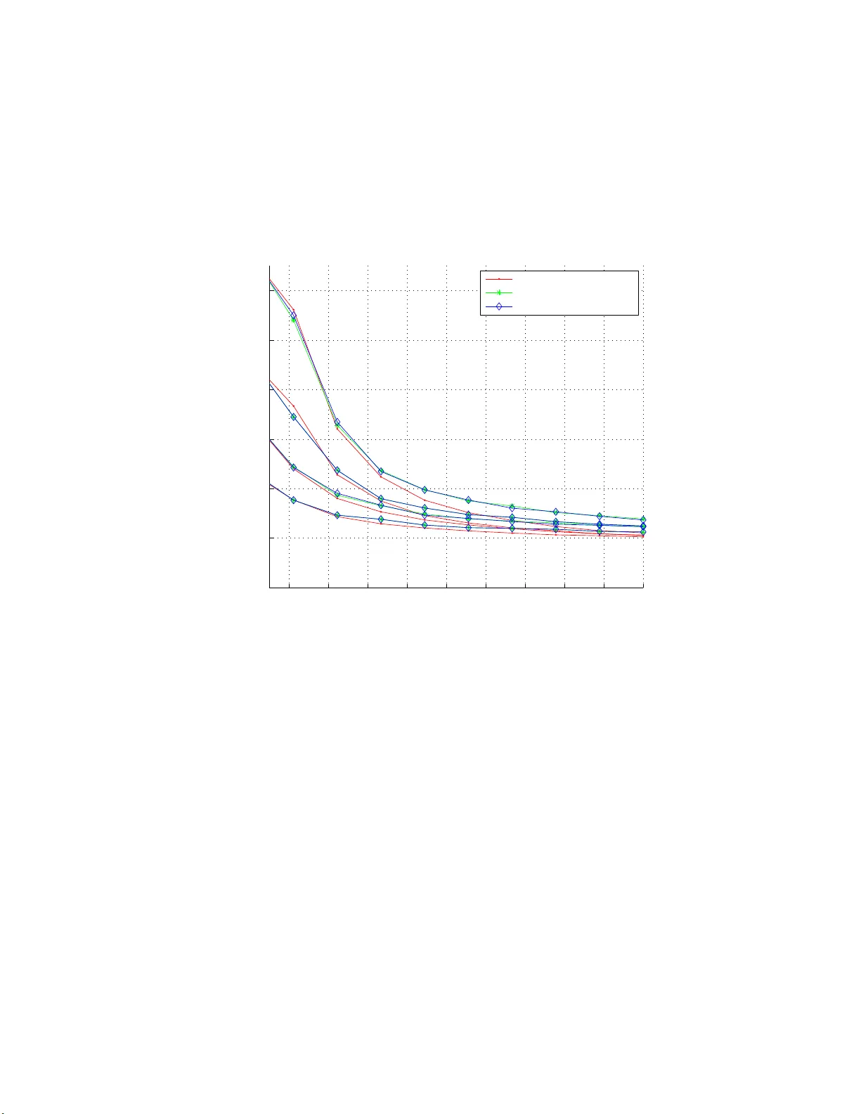
Randomized Sk etc hes of Con v ex Programs with Sharp Guaran tees Mert Pilanci ⋆ Martin J. W ain wrigh t ⋆, † { mert,wainw rig } @berkel ey.edu ⋆ Departmen t of Electrical Engineering and Computer Science † Departmen t of Statistics Univ ersit y of California, Berk eley April 30, 2014 Abstract Random pro jection (RP) is a classica l tec hnique for reducing stora g e and computatio na l costs. W e analyze RP-bas ed appr oximations of convex prog rams, in which the o riginal o pti- mization problem is approximated by the solution of a lo wer-dimensional problem. Such dimen- sionality reduction is ess ent ial in computation-limited settings , s inc e the complexity of g e neral conv ex progr amming can b e quite hig h (e.g., cubic for qua dr atic progra ms, a nd substantially higher for semideﬁnite programs). In addition to computational savings, rando m pro jection is also useful for reducing memory usa ge, and ha s useful pro pe r ties for pr iv acy-sensitive optimiza - tion. W e pr ov e that the approximation ratio of this pro c e dur e can b e bo unded in terms of the geometry of constraint set. F or a broa d cla ss of random pr o jections, including those based on v arious sub-Gaus sian distributions as w ell a s randomize d Hadamard and F ourier trans fo rms, the data matrix deﬁning the cost function can be pr o jected do wn to the statistica l dimension of the tangent cone of the constra int s at the original solution, whic h is often substantially smaller than the orig inal dimension. W e illustr ate co nsequences of our theory for v arious cases, including unconstrained and ℓ 1 -constrained least s q uares, supp ort vector machines, low-rank matrix esti- mation, a nd discuss implications on priv acy-sensitive o ptimiza tion and some connections with denoising and c ompressed sensing. 1 In tro duc tion Optimizing a con ve x fu n ction su b ject to constraints is fund amen tal to man y d isciplines in engi- neering, applied m athematics, and statistics [7, 28]. While most con ve x p rograms can b e solv ed in p olynomial time, the compu tational cost can still b e proh ib itiv e when the problem dimension and/or num b er of constrain ts are large. F or instance, although many qu adratic programs can b e solv ed in cubic time, this scaling m a y b e prohibitiv e w hen the dimension is on the order of millions. This t yp e of concern is only exacerbated for more sophisticated cone programs, such as second- order cone and semideﬁnite pr ograms. Con s equen tly , it is of great inte rest to deve lop m etho ds f or appro ximately solving such pr ograms, along w ith rigorous b ounds on the qualit y of the resu lting appro ximation. In this p ap er, w e analyze a p articular scheme for appr o ximating a con v ex program d eﬁned by minimizing a quadratic ob jectiv e function o v er an arb itrary conv ex set. T h e sc heme is simple to describ e and implement , as it is based on p erform in g a rand om pr o jectio n of the matrices and 1 v ectors deﬁning the ob jectiv e fu nction. Since the underlying constrain t set ma y b e arbitrary , our analysis encompasses many problem classes including quadratic p r ograms (with constrained or p enalized least-squares as a particular case ), as w ell as seco nd -order cone p rograms a n d semideﬁn ite programs (including lo w-rank matrix ap p ro ximation as a particular case). An in teresting class of suc h optimization p roblems arise in the conte xt of statistical estimation. Man y su ch p r oblems can b e formulated as estimating an u n kno wn parameter based on noisy linear measuremen ts, along with side information that the tru e parameter b elo n gs to a lo w-dimensional space. Examples of su c h lo w-d imensional structure include sp arse vec tors, low-rank matrices, dis- crete sets deﬁn ed in a com binatorial manner, as w ell as algebraic sets, including n orms f or ind ucing shrink age or smo othness. C on ve x relaxations provide a p rincipled wa y of deriving p olynomial-time metho ds for suc h problems [7], an d their s tatistical p erformance has b een extensiv ely studied o v er the past decade (see the pap ers [8, 35] for o verviews). F or many suc h problems, th e ambien t dimen- sion of th e p arameter is very large, and the num b er of samples can also b e large. In th ese cont exts, con v ex programs ma y b e d iﬃcult to solv e exactly , an d reducing the dimension and sample s ize by sk etc hing is a v ery attractiv e option. Our wo rk is related to a line of work on sk etc hing un constrained least-squares problems (e.g., see the p ap ers [15, 22, 6 ] and r eferences therein). The results giv en h ere generalizes this line of w ork by pro viding guarante es for the broader class of constrained quadr atic programs. In addition, our tec hniques are conv ex-analytic in nature, and by exploiting analytical tools from Banac h space geometry and empirical pro cess theory [12, 19, 18], lead to sharp er b ounds on the sk etc h size as w ell as sh arp er p robabilistic guarantee s. Our work also provi d es a u niﬁed view of b ot h least-squares sk etc hing [15, 22, 6] and compressed sensing [13, 14]. As we discuss in the sequel, v arious resu lts in compressed sensin g can b e understo o d as sp ecial cases of ske tc hed least-squares, in wh ic h the data matrix in the original quadratic program is the identi ty . In addition to redu cing compu tation and storage, random pro jection is also useful in the con text of p r iv acy pr eserv atio n. Many t yp es of mo d ern data, including ﬁn an cial r ecords and m edical tests, ha ve asso ciated p riv acy concerns. Random p ro jectio n allo ws for a ske tched v ersion of the data set to b e stored, but such that there is a v anishingly small amount of information ab out any giv en data p oint . Our theory shows that this is still p ossib le, w hile still solving a conv ex program d eﬁned by the data set up to δ -accuracy . In this w ay , we sharp en some results by Zhou and W asserm an [37] on priv acy-preserving rand om pro jections for sparse regression. O u r theory p oin ts to an in teresting dic hotom y in priv acy sensitiv e optimizat ion p roblems b ased on the trade-oﬀ b et wee n the co mp lexit y of the constrain t set and m utual information. W e show th at if the c onstraint set is simp le enough in terms of a statistical measur e, priv acy sensitiv e optimization can b e done with arbitrary accuracy . The remainder of this pap er is organized as follo ws. W e b egin in S ection 2 with a more precise form ulation o f t he problem, an d th e statemen t of our main results. In S ection 3, w e deriv e co rollaries for a num b er of concrete classes of problems, and pr o vide v arious simulatio ns that d emonstrate the close agreemen t b et w een th e th eoretical pr edictions and b ehavior in pr actice. Sections 4 and Section 5 are devo ted to the pr o ofs our main results, and w e conclude in Section 6. P arts of the results give n h ere are to app ea r in the conference form at the In ternational Symp osium on Information Theory (2014) . 2 2 Statemen t of main results W e b egin b y formulating th e problem analyzed in this pap er, b efore turning to a statemen t of our main results. 2.1 Problem form ulation Consider a con v ex program of the form x ∗ ∈ arg min x ∈C k Ax − y k 2 2 | {z } f ( x ) , (1) where C is some conv ex subs et of R d , and y ∈ R n A ∈ R n × d are a data vect or and data matrix, resp ectiv ely . Our goal is to obtai n an δ -optimal solutio n to this problem in a compu tationally simpler manner, and we do so b y pro jecting the p r oblem in to R m , where m < n , via a sk e tching matrix S ∈ R m × n . In particular, consider the sketche d pr oblem b x ∈ arg min x ∈C k S ( Ax − y ) k 2 2 | {z } g ( x ) . (2) Note that by the optimalit y and f easibility of x ∗ and b x , resp ect ively , for the original problem (1), w e alw ays hav e f ( x ∗ ) ≤ f ( b x ). Accordingly , we say that b x is an δ -optima l appr oximat ion to the original problem (1) if f ( b x ) ≤  1 + δ  2 f ( x ∗ ) . (3) Our main result c haracterize s the n umb er of samp les m required to achiev e this b oun d as a function of δ , and other problem parameters. Our analysis inv olv es a natur al geometric ob ject in conv ex analysis, namely the tangen t cone of the constrain t set C at the optim um x ∗ , giv en by K : = clcon v  ∆ ∈ R d | ∆ = t ( x − x ∗ ) for some t ≥ 0 and x ∈ C } , (4) where clcon v d enotes th e closed conv ex hull. Th is set arises naturally in the con ve x optimalit y conditions for th e original problem (1 ): an y v ector ∆ ∈ K deﬁnes a feasible direction at the optimal x ∗ , and optimalit y m eans that it is imp ossible to decrease the cost function by mo ving in d irections b elonging to the tangen t cone. W e u se A K to d enote the linearly transformed cone { A ∆ ∈ R n | ∆ ∈ K} . O u r main results in vo lve measures of the “size” of this transformed cone when it is intersec ted with the Euclidean sphere S n − 1 = { z ∈ R n | k z k 2 = 1 } . In particular, w e d eﬁne Gaussian width of the set A K ∩ S n − 1 via W ( A K ) : = E g  sup z ∈ A K∩S n − 1   h g , z i    (5) where g ∈ R n is a n i.i.d. sequen ce of N (0 , 1) v ariables. This complexit y measure pla ys an imp ortan t role in Banac h sp ace theory , learning th eory and statistics (e.g., [31 , 19, 5]). 3 2.2 Guaran tees for sub-Gaussian sketc hes Our ﬁ rst main result pr o vides a relation b et ween the suﬃcien t sk etc h size and Gaussian complexit y in the case of sub-Gaussian sk etc hes. In particular, we sa y that a r o w s i of the sket ching matrix is σ -sub- Gaussian if it is zero-mean, and if for any ﬁxed unit v ector u ∈ S n − 1 , w e ha ve P  |h u, s i i| ≥ t ] ≤ 2 e − nt 2 2 σ 2 for all t ≥ 0. (6) Of course, this condition is satisﬁed by the s tand ard Gaussian sketc h ( s i ∼ N (0 , I n × n )). In addi- tion, it holds for v arious other sk etc hing matrices, including random matrices w ith i.i.d. Bernoulli elemen ts, random matrices with ro ws drawn u niformly from the rescaled u nit sp here, and so on. W e say that the sk etc hing matrix S ∈ R m × n is d ra wn from a σ -sub-Gaussian ensemble if eac h r ow is σ -sub-Gaussian in the pr eviously deﬁn ed sense (6). Theorem 1 (Guarantee s for s u b-Gaussian pro jections) . L et S ∈ R m × n b e dr aw n fr om a σ - sub- Gaussian ensemble. Then ther e ar e universal c onstants ( c 0 , c 1 , c 2 ) such that, for any toler anc e p ar ameter δ ∈ (0 , 1) , g iven a ske tch si ze lower b ounde d as m ≥ c 0 δ 2 W 2 ( A K ) , (7) the appr oximate solution b x is guar ante e d to b e δ - optimal (3) for the original pr o gr am with pr ob ability at le ast 1 − c 1 e − c 2 mδ 2 . As will b e clariﬁed in examples to follo w, the sq u ared width W 2 ( A K ) scales p rop ortionally to the statistica l dimension, or n umb er of degrees of freedom in the set A K ∩ S n − 1 . Consequen tly , up to constan t factors, Theorem 1 guaran tees th at we can p ro ject down to the statistical dimen sion of the problem while preserving δ -optimalit y of the solution. This fact has an interesting coroll ary in the con text of priv acy-sensitiv e optimizatio n. Sup p ose that we mo d el the data m atrix A ∈ R n × d as b eing random, and our goal is to s olve the original con v ex pr ogram (1) up to δ -accuracy while rev ealing as little as possib le ab out the individual entries of A . By Theorem 1 , w henev er the sketc h dimens ion satisﬁes the lo w er b ound (7), the ske tc hed data m atrix S A ∈ R m × d suﬃces to solv e the original p rogram up to δ -accuracy . W e can th us ask ab out ho w muc h information p er en try of A is r etained by the sk etc hed data m atrix. On e w ay in whic h to do so is by compu ting the m utual information p er symbol, namely I ( S A ; A ) nd = 1 nd  H ( A ) − H ( A | S A )  , where the rescaling is c hosen since A has a total of nd en tries. This quan tit y wa s stud ied by Zhou and W asserman [37] in the con text of priv acy-sensitiv e sparse regression, in wh ic h C is an ℓ 1 -ball, to b e discussed at m ore in length in Section 3.2. In our setting, we ha ve the follo wing more generic corollary of Theorem 1: Corollary 1. L e t the entries of A b e dr aw n i.i.d. fr om a distribution with ﬁnite varianc e γ 2 . Byusing m = c 0 δ 2 W 2 ( A K ) r andom Gaussian pr oje ctions, we c an ensur e that I ( S A ; A ) nd ≤ c 0 δ 2 W 2 ( A K ) n log(2 π eγ 2 ) , (8) and that the sketche d solution is δ - optimal with pr ob ability at le ast 1 − c 1 e − c 2 mδ 2 . 4 Note that the inequalit y W 2 ( A K ) ≤ n alw a ys holds. Ho wev er, for man y pr oblems, w e hav e the m uch s tronger guarantee W 2 ( A K ) = o ( n ), in whic h case the b oun d (8) guaran tees that the mutual information p er sym b ol is v anishing. There are v arious concrete p roblems, as discussed in Section 3, for whic h this t yp e of scaling is reasonable. T h us, for any ﬁxed δ ∈ (0 , 1), we are guarant eed a δ -optimal solution with a v anishing m utual in formation p er sym b ol. Corollary 1 follo ws by a straigh tforw ard combinatio n of past wo rk [37] with Theorem 1. Zhou and W asserman [37] sh o w that u nder the stated conditions, for a stand ard i.i.d. Gauss ian sk etc hing matrix S , the m utual information rate p er symb ol is u pp er b ounded as I ( S A ; A ) nd ≤ m 2 n log(2 π eγ 2 ) . Substituting in the stated c hoice of m and applying Theorem 1 yields the claim. 2.3 Guaran tees for randomized orthogonal systems A p ossible disadv antag e of using sub-Gaussian s ketc hes is that it requires p erf orming matrix-v ector m ultiplications with unstr u ctured random matrices; suc h multiplic ations r equire O ( mnd ) time in general. Our second main result applies to sk etc hes based on a r andomize d orth onormal system (R OS), for wh ic h matrix multiplic ation can b e p erformed m uch more qu ic kly . In order to deﬁne a r andomized orthonormal system, w e b egin by with an orthonormal matrix H ∈ R n × n with en tries H ij ∈ {− 1 √ n , 1 √ n } . A standard cla ss of such matrice s is provided b y the Hadamard basis, for whic h m atrix-v ector multiplicat ion can b e p erform ed in O ( n log n ) time. Another p ossible c hoice is the F our ier basis. Based on any suc h matrix, a sk etc hing matrix S ∈ R m × n from a R OS ensemble is ob tained b y sampling i.i.d. ro ws of the form s i = √ nD H T p i , where the random ve ctor p i ∈ R n is c hosen un iformly at r andom from the s et of all n canonical basis v ectors, and D = diag( ν ) is a diagonal matrix of i.i.d. Rademacher v ariables ν ∈ {− 1 , +1 } n . With the base matrix H chosen as the Hadamard or F our ier basis, then for any ﬁxed v ector x ∈ R n , the pro d u ct S x can b e compu ted in O ( n log m ) time (e.g., see the pap er [2] for details). Hence the ske tc hed data ( S A, S y ) can b e formed in O ( d n log m ) time, w h ic h scales almost linearly in the input size dn . Our main result for ran d omized orthonormal systems inv olv es the S -Gaussian width of the set A K ∩ S n − 1 , giv en by W S ( A K ) : = E g ,S h sup z ∈ A K∩S n − 1    h g , S z √ m i    i . (9) As will b e clear in the corollaries to f ollo w, in many cases, the S -Gaussian w idth is equiv alen t to the ord inary Gaussian w idth (5) up to n umerical constan ts. It also inv olv es the R ad emacher width of the set A K ∩ S n − 1 , giv en by R ( A K ) = E ε  sup z ∈ A K∩S n − 1   h z , ε i    , (10) where ε ∈ {− 1 , +1 } n is an i.i.d. v ector of Rademac her v ariables. 5 Theorem 2 ( Guarantees for randomized orthonormal system) . L et S ∈ R m × n b e dr awn fr om a r and omize d orthono rmal system (R OS). Then given a sample size m lower b ounde d as m log m > c 0 δ 2  R 2 ( A K ) + log n  W 2 S ( A K ) , (11) the appr oximate solution b x is guar ante e d to b e δ - optimal (3) for the original pr o gr am with pr ob ability at le ast 1 − c 1 ( mn ) 2 − c 1 exp  − c 2 mδ 2 R 2 ( A K )+log( mn )  . The r equired pro jectio n dimension (11) for R OS s k etc hes is in general larger than that required for sub-Gaussian sketc hes, due to the presence of the additional pre-factor R 2 ( A K ) + log n . F or certain t yp es of cones, w e can use m ore sp ecialized tec hniques to remo v e this pr e-factor, so that it is not alw a ys r equired. The details of these arguments are giv en in Section 5, and w e p ro vide some illustrativ e examples of suc h sharp ened results in the corollaries to follo w. Ho we ver, the p oten tially larger pro jection d imension is oﬀset b y the m uc h lo w er compu tational complexit y of forming matrix v ector pr o ducts using the R OS sk etc hin g matrix. 3 Some concrete instan tiations Our t wo main theorems are general results that app ly to any c hoice of the conv ex constraint set C . W e no w tur n to some consequences of T heorems 1 and 2 for more sp eciﬁc classes of problems, in whic h the geometry ente rs in diﬀerent wa ys. 3.1 Unconstrained least squares W e b egin with the simplest p ossible c hoice, namely C = R d , whic h leads to an unconstrained least squares problem. This class of p r oblems h as b een studied extensiv ely in past w ork on least-square sk etc hing [22]; our deriv atio n h er e provides a sharp er resu lt in a more d irect m anner. A t least in tuitiv ely , giv en the d ata matrix A ∈ R n × d , it should b e p ossible to redu ce the dimens ionalit y to the rank of the data matrix A , while preserving th e accuracy of the solution. In man y cases, the quan tit y rank( A ) is sub stan tially smaller than max { n, d } . The follo wing corollaries of T heorem 1 and 2 conﬁrm this in tuition: Corollary 2 (App ro ximation guarantee for unconstrained least squares) . Consider the c ase of unc onstr aine d le ast squar es with C = R d : (a) Given a sub-Gaussian sketch with dimension m > c 0 rank( A ) δ 2 , the sketche d solution is δ - optimal (3 ) with pr ob ability at le ast 1 − c 1 e − c 2 mδ 2 . (b) Given a R OS sketch with dimension m > c ′ 0 rank( A ) δ 2 log 4 ( n ) , the sketche d solution is δ -optimal (3) with pr ob ability at le ast 1 − c 1 e − c 2 mδ 2 . This corollary impro ve s kno wn results b oth in the probabilit y estimate and r equired samples, in par- ticular previous results hold only with constant probabilit y; see the pap er [22] for an o ve rv iew of suc h results. Note that the total computational complexit y of compu ting S A and solving the sk etc hed least squ ares problem, for ins tance via QR decomp osition [16], is of the order O ( n dm + md 2 ) for sub-Gaussian sk etc hes, and of the order O ( nd log ( m ) + md 2 ) fo r R OS sk etc hes. Consequentl y , by us- ing R OS sk etc hes, the o v erall complexit y of computing a δ -app ro ximate least squ ares solution with 6 exp onenti ally high p robabilit y is O (r ank( A ) d 2 log 4 ( n ) /δ 2 + nd log(rank( A ) /δ 2 )). In man y ca ses, this complexit y is s ubstant ially low er than d ir ect computation of the solution via QR decomp osition, whic h would r equire O ( nd 2 ) op erations. Pr o of. Sin ce C = R d , the tangen t cone K is all of R d , and the set A K is the image of A . Th us, w e ha ve W ( A K ) = E  sup u ∈ R d h Au, g i k Au k 2  ≤ p rank( A ) , (12) where the inequalit y f ollo ws fr om the the fact that the image of A is at most rank( A )-dimensional. Th u s, the sub-Gaussian b ound in part (a) is an immediate consequence of Theorem 1. T u rning to p art (b ), an application of Theorem 2 will lead to a sub-optimal r esult inv olving (rank( A )) 2 . In Section 5.1, w e sh ow h o w a reﬁned argumen t w ill lead to b ound stated here. In order to inv estigat e the theoretical prediction of Corollary 2, w e p erformed some simple sim ulations on rand omly generated p roblem in stances. Fixing a d imension d = 500, we f ormed a random ensemble of least-squares pr oblems by ﬁrst generating a rand om d ata matrix A ∈ R n × 500 with i.i.d. standard Gaussian entries. F or a ﬁ xed rand om v ector x 0 ∈ R d , w e then computed the data v ector y = Ax 0 + w , wh ere the noise v ector w ∼ N (0 , ν 2 ) where ν = √ 0 . 2. Giv en this r andom en sem ble of problems, we computed the pro jected d ata matrix-vec tor pairs ( S A, S y ) using Gaussian, Rademac her , and randomized Hadamard ske tc hin g matrices, and then solved the pro jected con v ex program. W e p erformed this exp eriment for a range of diﬀeren t prob lem sizes n ∈ { 1024 , 2048 , 40 9 6 } . F or an y n in this set, we ha ve rank( A ) = d = 500, with high probabilit y o v er the c h oice of ran d omly sampled A . Supp ose that we c ho ose a pro jection dimension of the f orm m = 1 . 5 αd , w here the con trol parameter α r anged o v er the in terv al [0 , 1]. Corollary 2 p redicts that the approxima tion err or should con v erge to 1 under this scaling, for eac h c h oice of n . Figure 1 sho ws th e r esults of these exp eriments, plotting the approxi mation ratio f ( b x ) /f ( x ∗ ) v ersus the con trol p arameter α . Consistent with C orollary 2, regardless of th e c hoice of n , once the pr o jecti on dimens ion is a s u itably large multiple of rank( A ) = 500, the appr o ximation qualit y b ecomes v ery go o d. 3.2 ℓ 1 -constrained least squares W e no w turn a constrained form of least -squ ares, in which the geometry of the tangen t co ne en ters in a more in teresting w ay . In particular, consider the follo wing ℓ 1 -constrained least squares program, kno wn as the Lasso [9, 34] x ∗ ∈ arg min k x k 1 ≤ R k Ax − y k 2 2 . (13) It is is widely used in signal pro cessing and statistics for sp arse signal reco v ery and appr o ximation. In this section, we sho w that as a corollary of Theorem 1, this quadratic program can b e sk etc hed logarithmically in dimension d when the o ptimal solution to the original problem is sparse. In particular, assuming that x ∗ is unique, we let k den ote the num b er of non-zero co eﬃcients of the un ique solution to the ab o ve pr ogram. (When x ∗ is not unique, w e let k denote th e minimal 7 0 0.1 0.2 0.3 0.4 0.5 0.6 0.7 0.8 0.9 1 10 20 30 40 50 60 70 C o n t r o l p a r a m e t e r α A p p r o x . r a t i o f ( x ) / f ( x * ) U n c o n s t r a i n e d L e a s t S q u a r e s : d = 5 0 0 n=4096 n=2048 n=1024 Randomized Hadamard Gaussian Rademacher Figure 1. Comparison o f Ga us sian, Rademacher and ra ndo mized Hadamard sketc hes for unco n- strained lea st squares. Each curve plots the a pproximation ra tio f ( b x ) /f ( x ∗ ) versus the control parameter α , av erage d over T tr ial = 1 00 trials, for pr o jection dimensions m = 1 . 5 αd a nd for problem dimensions d = 500 and n ∈ { 1024 , 2048 , 4 0 96 } . cardinalit y among all optimal v ectors). Deﬁne the ℓ 1 -restricted eigen v alues of the giv en data matrix A as γ − k ( A ) : = min k z k 2 =1 k z k 1 ≤ 2 √ k k Az k 2 2 , and γ + k ( A ) : = max k z k 2 =1 k z k 1 ≤ 2 √ k k Az k 2 2 . (14) Corollary 3 (Appro ximation guaran tees for ℓ 1 -constrained least squares) . Consider the ℓ 1 -c onstr aine d le ast squar es pr oblem (13) : (a) F or sub-Gaussian sketches, a sketch dimension lower b ounde d by m ≥ c 0 δ 2 min  rank( A ) , max j =1 ,...,d k a j k 2 2 γ − k ( A ) k log ( d )  (15) guar ant e es that the sk e tche d solution is δ -optimal (3) with pr ob ability at le ast 1 − c 1 e − c 2 mδ 2 . (b) F or ROS sketches, a sk e tch dimension lower b ounde d by m > c ′ 0 δ 2 log 4 ( n ) min  rank( A ) ,  max j k a j k 2 2 γ − k ( A ) k log ( d )  2 log 4 ( n ) ,  γ + k ( A ) γ − k ( A )  2 k log ( d )  (16) guar ant e es that the sk e tche d solution is δ -optimal (3) with pr ob ability at le ast 1 − c 1 e − c 2 mδ 2 . 8 W e note that p art (a) of this corollary impro ves the resu lt of Zhou et al. [37 ], which establishes consistency of Lasso with a Gauss ian sketc h dimension of the order k 2 log( dnk ), in con trast to the k log ( d ) requirement in the b ound (15). T o b e more p recise, these tw o r esults are slightl y diﬀeren t, in that the result [37] fo cuses on sup p ort reco v ery , whereas Corollary 3 guarant ees a δ -accurate appro ximation of the cost fu nction. Let u s consid er th e complexit y of solving the s k etc hed p roblem u sing d iﬀeren t metho ds. I n the regime n > d , the complexity of solving the original Lasso problem as a linearly constrained quadratic pr ogram via in terior p oint solv ers is O ( nd 2 ) p er iteration (e.g., see Nestero v and Ne- miro vski [30 ]). Thus, computing the sketc h ed d ata and solving the sk etc hed Lasso pr oblem requires O ( ndm + md 2 ) op erations for sub-Gaussian sk etc hes, and O ( nd log ( m ) + md 2 ) for R OS sk etc hes. Another p opular c hoice for solving th e Lasso problem is to use a ﬁrst-order algorithm [29]; suc h algorithms requir e O ( nd ) op erations p er iteration, and yield a solution that is O (1 /T )-optimal within T iterations. If we apply suc h an algorithm to th e sketc hed v ersion for T steps, th en we obtain a v ector su c h that f ( b x ) ≤ (1 + δ ) 2 f ( x ∗ ) + O ( 1 T ) . Ov erall, obtaining this guarantee requires O ( ndm + mdT ) op erations for sub-Gaussian sk etc hes, and O ( nd log( m ) + mdT ) op erations for R OS sketc h es. Pr o of. Let S denote the su pp ort of the optimal solution x ∗ . The tangen t co ne to the ℓ 1 -norm constrain t at th e optimum x ∗ tak es the f orm K =  ∆ ∈ R d | h ∆ S , b z S i + k ∆ S c k 1 ≤ 0 } , (17) where b z S : = sign( x ∗ S ) ∈ {− 1 , +1 } k is the sign v ector of the optimal solution on its su pp ort. By the triangle inequalit y , any v ector ∆ ∈ K satisﬁes the inequalit y k ∆ k 1 ≤ 2 k ∆ S k 1 ≤ 2 √ k k ∆ S k 2 ≤ 2 √ k k ∆ k 2 . (18) If k A ∆ k 2 = 1, then by th e deﬁnition (14), w e also hav e the upp er b ound k ∆ k 2 ≤ 1 q γ − k ( A ) , whence h A ∆ , g i ≤ 2 p | S | k ∆ k 2 k A T g k ∞ ≤ 2 p | S | k A T g k ∞ q γ − k ( A ) . (19) Note that A T g is a d -dimensional Gaussian v ector, in wh ic h the j th -en try has v ariance k a j k 2 2 . Consequent ly , inequalit y (19 ) com bined with stand ard Gaussian tail b ound s [19] imply that W ( A K ) ≤ 6 p k log( d ) max j =1 ,...,d k a j k 2 q γ − k ( A ) . ( 20) Com bined with the b ound fr om Corollary 2, also applicable in this setting, the claim (15) follo ws. T u rning to part (b), the ﬁrs t lo w er bou n d in vol ving rank( A ) follo ws from Corollary 2. The second lo w er b ound follo w s as a corollary of Theorem 2 in application to the Lasso; see App endix A for th e calculations. Th e third lo w er b ound follo ws by a sp ecialized argum en t giv en in Section 5.3. 9 In order to inv estigate the pr ediction of Corollary 3, w e generated a r andom en s em ble of spars e linear regression problems as follo ws. W e ﬁrst generated a data matrix A ∈ R 4096 × 500 b y sampling i.i.d. standard Gaussian entries, and then a k ′ -sparse b ase v ector x 0 ∈ R d b y c ho osing a uniformly random subset S of size k ′ = d/ 10, and setting its en tries to in {− 1 , +1 } ind ep enden t and equiprob- ably . Finally , w e formed the data vect or y = Ax 0 + w , where the n oise v ector w ∈ R n has i.i.d. N (0 , ν 2 ) en tries. 0.1 0.2 0.3 0.4 0.5 0.6 0.7 0.8 0.9 1 0.8 1 1.2 1.4 1.6 1.8 2 C o n t r o l p a r a m e t e r α A p p r o x . r a t i o f ( x ) / f ( x * ) L A S S O : d = 5 0 0 R=1 R=5 R=10 R=20 Randomized Hadamard Gaussian Rademacher Figure 2. Comparis o n of Gaussian, Radema cher and r andomized Hadamard sketc hes fo r the Las so progra m (13). E ach curve plots the approximation ratio f ( b x ) /f ( x ∗ ) v er sus the c o ntrol parameter α , av erag e d ov er T tr ial = 1 00 trials, for pro jection dimensions m = 4 α k x ∗ k 0 log d , problem dimensions ( n, d ) = (40 96 , 500), and ℓ 1 -constraint radius R ∈ { 1 , 5 , 10 , 20 } . In o ur exp eriment s, we solv ed the Lasso (1 3) with a c hoice of radius parameter R ∈ { 1 , 5 , 10 , 20 } , and set k = k x ∗ k 0 . W e then set the pro ject ion dimension m = 4 k log d where α ∈ (0 , 1) is a control parameter, and solv ed the s k etc hed Lasso for Gaussian, R ad emacher and randomized Hadamard sk etc hing matrices. O u r theory predicts that the appro ximation ratio should tend to one as the con trol parameter α in creases. The results are plotted in Figure 2, and conﬁrm this qualitativ e prediction. 3.3 Compressed sensing and noise folding It is w orth n oting that v arious compressed sens in g results can b e reco ve red as a sp ecia l case of Corollary 3—m ore pr ecisely , one in whic h the “data matrix” A is simply the ident ity (so that n = d ). With this c hoice, the original p roblem (1) corresp ond s to the classical denoising pr oblem, 10 namely x ∗ = arg min x ∈C k x − y k 2 2 , (21) so that the cost function is simply f ( x ) = k x − y k 2 2 . With the c hoice of constraint set C = {k x k 1 ≤ R } , the optimal solution x ∗ to the original p roblem is u n ique, and can b e obtained by p erformin g a co ord inate-wise soft-thresholding op eratio n on the data v ector y . F or this c hoice, the sketc hed v ersion of the de-noising p roblem (21) is giv en by b x = arg min x ∈C k S x − S y k 2 2 (22) Noiseless v ersion: In the noiseless v ersion of compressed sensing, we hav e y = ¯ x ∈ C , and hen ce the optimal solution to the original “denoising” problem (21) is giv en by x ∗ = ¯ x , with optimal v alue f ( x ∗ ) = k x ∗ − ¯ x k 2 2 = 0 . Using the sk etc hed data vec tor S ¯ x ∈ R m , w e can solv e th e sk etc hed program (22). If doing so yields a δ -appro ximation b x , then in this sp ecia l case, we are guaranteed that k b x − ¯ x k 2 2 = f ( b x ) ≤ (1 + δ ) 2 f ( x ∗ ) = 0 , (23) whic h implies th at we h av e exact reco v ery—th at is, b x = ¯ x . Noisy vers ions: In a more general setting, we observe th e v ector y = ¯ x + w , where ¯ x ∈ C and w ∈ R n is some t yp e of observ ation noise. The sk etc hed observ ation mo del then tak es th e form S y = S ¯ x + S w, so that the sk etc hing matrix is applied to b oth the true v ect or ¯ x and th e noise v ector w . This set-up corresp onds to an instance of compr essed sen sing with “folded” n oise (e.g., see the p ap ers [3, 1]), whic h some argue is a more realistic set-up for compressed sensing. In this conte xt, our r esu lts imply that the sk etc hed v ersion s atisﬁes the b oun d k b x − y k 2 2 ≤  1 + δ  2 k x ∗ − y k 2 2 . (24) If w e think of y as an appr o ximately sparse ve ctor and x ∗ as the b est appro ximation to y f rom the ℓ 1 -ball, th en this b oun d (24) guarante es that we reco v er a δ -approxima tion to the b est sp arse appro ximation. Moreo v er, th is b oun d shows that th e compr essed sensing error should b e closely related to the error in denoising, as has b een made precise in recen t w ork [14]. Let us summarize these conclusions in a corollary: Corollary 4. Consider an instanc e of the denoising pr oblem (21) when C = { x ∈ R n | k x k 1 ≤ R } . (a) F or sub- Gaussian sketches with pr oje ction dimension m ≥ c 0 δ 2 k x ∗ k 0 log d , we ar e g uar ante e d exact r e c overy i n the noiseless c ase (23) , and δ -appr oxima te r e c overy (24) in the noisy c ase, b oth with pr ob ability at le ast 1 − c 1 e − c 2 mδ 2 . 11 (b) F or R OS sketches, the same c onclusions hold with pr ob ability 1 − e − c 1 mδ 2 log 4 n using a sketch dimension m ≥ c 0 δ 2 min  k x ∗ k 0 log 5 d, k x ∗ k 2 0 log d  . (25) Of course, a more general v ersion of this corollary holds for an y con vex constrain t set C , in- v olving the Gauss ian/Rademac her width f unctions. In th is more setting, the corollary generalizes results b y C h andrasek aran et al. [8], w ho stu died r andomized Gaussian sk etc hes in application to atomic n orms, to other types of sk etc hing matrices and other types of constraints. They provi d e a num b er of calculations of width s for v arious atomic norm constraint sets, including p erm uta- tion and orthogonal matrices, and cut p olytopes, w hic h can b e used in conju n ction with the more general form of Corollary 4. 3.4 Suppor t v ector machi ne classiﬁcation Our theory also has applications to learnin g linear classiﬁers based on lab eled samples. In the con text of bin ary classiﬁcation, a lab eled sample is a p air ( a i , z i ), w here th e v ector a i ∈ R n represent s a col lection of features, and z i ∈ {− 1 , +1 } is the associated class lab el. A linear classiﬁer is sp eciﬁed b y a fun ction a 7→ sign( h w , a i ) ∈ {− 1 , + 1 } , where w ∈ R n is a w eigh t v ector to b e estimated. Giv en a set of lab elled patterns { a i , z i } d i =1 , the supp ort ve ctor m achine [10, 33] estimates the w eigh t v ector w ∗ b y minimizing the f unction w ∗ = arg min w ∈ R n n 1 2 C d X i =1 g ( y i , h w , a i i ) + 1 2 k w k 2 2 o . (26) In this form ulation, the squared hinge loss g ( w ) : = (1 − y i h w, a i i ) 2 + is used to measure the p erfor- mance of the classiﬁer on sample i , and the quadratic p enalt y k w k 2 2 serv es as a form o f reg u larization. By considering the d ual of this p roblem, w e arriv e at a least-squares problem that is amenable to our sk etc hing techniques. Let A ∈ R n × d b e a matrix with a i ∈ R n as its i th column, and let D = diag( z ) ∈ R d × d b e a diagonal matrix and let B T = [( AD ) T 1 C I ]. Wi th this notation, th e asso ciated dual problem (e.g. see the pap er [20]) tak es th e form x ∗ : = arg min x ∈ R d k B x k 2 2 suc h that x ≥ 0 and d P i =1 x i = 1. (27) The optimal solution x ∗ ∈ R d corresp onds to a v ector of w eigh ts asso ciated with the samp les: it sp eci ﬁ es the op timal SVM weig ht v ector via w ∗ = P d i =1 x ∗ i z i a i . It is often the case that the dual solution x ∗ has r elativ ely f ew non-zero co eﬃcien ts, corr esp onding to samples that lie on th e so-calle d margin of the supp ort vecto r mac hin e. The sk etc hed ve rsion is then giv en by b x : = arg min x ∈ R d k S B x k 2 2 suc h that x ≥ 0 and d P i =1 x i = 1. (28) The simplex constrain t in the qu ad r atic program (27), although not identica l to an ℓ 1 -constrain t, leads to similar scaling in terms of the ske tc h dimension. 12 Corollary 5 (Sk etc h dimensions for supp ort v ector mac hines) . Given a c ol le ction of lab ele d samples { ( a i , z i ) } d i =1 , let k x ∗ k 0 denote the numb er of samples on the mar gin in the SVM solution (27 ) . Then given a sub-Gaussian sketch with dimension m ≥ c 0 δ 2 k x ∗ k 0 log( d ) max j =1 ,...,d k a j k 2 2 γ − k ( A ) , (29) the sketche d solution (28) is δ -optimal with pr ob ability at le ast 1 − c 1 e − c 2 mδ 2 . W e omit the pro of, as the calculations sp ecia lizing fr om Theorem 1 are essentia lly th e same as those of Corollary 3. The computational complexit y of solving the SVM problem as a linearly constrained quadratic problem is same with the Lasso problem, hence same conclusions apply . 0.1 0.2 0.3 0.4 0.5 0.6 0.7 0.8 0.9 1 5 10 15 20 25 30 C o n t r o l p a r a m e t e r α A p p r o x . r a t i o f ( x ) / f ( x * ) Support Vector Machine d=4096 d=2048 d=1024 Randomized Hadamard Gaussian Rademacher Figure 3. Compariso n o f Gaussian, Rademacher and randomized Hadamard sketc hes for the sup- po rt vector machine (27). Each curve plo ts the approximation ratio f ( b x ) /f ( x ∗ ) versus the co nt ro l parameter α , averaged over T tr ial = 100 trials, for pro jection dimensions m = 5 α k x ∗ k 0 log d , and problem dimensions d ∈ { 1024 , 20 48 , 4096 } . In order to study the prediction of Corollary 5, w e generated some classiﬁcat ion exp eriment s, and tested th e p er f ormance of the sket ching pr o ce d ure. Consider a t w o-comp onent Gaussian mixture mo del, based on the comp on ent distributions N ( µ 0 , I ) and N ( µ 1 , I ), where µ 0 and µ 1 are uniformly distributed in [ − 3 , 3]. P lacing equal wei ghts on eac h comp onent, we d ra w d samp les f rom this mixture distrib ution, and then use the resulting data to solv e the SVN du al program (27), thereb y obtaining an op timal linear decision b oun dary sp eciﬁed b y the v ector x ∗ . The num b er of non-zero en tries k x ∗ k 0 corresp onds to the num b er of examples on the d ecision b oundary , kno wn as sup p ort 13 v ectors. W e then solv e the sk etc hed v ersion (28), using either Gaussian, Rademac her or randomized Hadamard ske tc hes, and us in g a pro jection dimens ion scaling as m = 5 α k x ∗ k 0 log d , where α ∈ [0 , 1] is a con trol parameter. W e rep eat this exp erimen t for pr oblem dimensions d ∈ { 102 4 , 2048 , 4096 } , p erformin g T trial = 100 trials for eac h c hoice of ( α, d ). Figure 3 shows plots of the approxima tion r atio ve rs us the con trol p arameter. Eac h b u ndle of curv es corresp onds to a diﬀeren t pr ob lem dimension, and has thr ee curves for the three diﬀeren t sk etc h types. Consistent with th e theory , in all cases, the approximat ion error app r oac hes one as α scales upw ards. It is worth while noting that similar sketc h ing tec hn iques can b e applied to other optimization problems that inv olv e the u nit simplex as a constraint. Another in stance is the Mark owit z formu- lation of the p ortfolio op timization pr oblem [23]. Here the goal is to estimate a vecto r x ∈ R d in the un it simplex, corresp onding to non -n egativ e w eigh ts asso ci ated with eac h of d p ossible assets, so as to minimize the v ariance of the return sub ject to a lo w er b ound on the exp ected retur n. More precisely , w e let µ ∈ R d denote a v ector corresp onding to mean return asso ciated with the assets, and w e let Σ ∈ R d × d b e a symmetric, p ositiv e s emideﬁnite matrix, corresp onding to the co v ariance of the returns . Typical ly , th e mean vect or and cov ariance matrix are estimated from data. Give n the pair ( µ, Σ), the Mark o witz allo cation is giv en by x ∗ = arg min x ∈ R d x T Σ x suc h that h µ, x i ≥ γ , x ≥ 0 and P d j =1 x j = 1. (30) Note that this problem can b e w r itten in the same form as the S VM, since the co v ariance matrix Σ  0 can b e factorize d as Σ = A T A . Wheneve r the exp ected r eturn constraint h µ, x i ≥ γ is activ e at the solution, the tangen t cone is give n by K =  ∆ ∈ R d | h µ, ∆ i ≥ 0 , d X j =1 ∆ j = 0 , ∆ S c ≥ 0 } where S is th e supp ort of x ∗ . Th is tangen t cone is a subs et of the tangen t cone for the SVM, and hence the b ound s of Corollary 5 also apply to the p ortfolio optimization p roblem. 3.5 Matrix estimation with n uclear norm regularization W e now turn to the use of sket ching for matrix estimation problems, and in p articular those that in vo lve nuclea r norm constraints. Let C ⊂ R d 1 × d 2 b e a conv ex sub s et of the space of all d 1 × d 2 matrices. Man y matrix estimation problems can b e written in the general form min X ∈C k y − A ( X ) k 2 2 where y ∈ R n is a data vecto r, and A is a linear op erator fr om R d 1 × d 2 to R n . Letting ve c denote the v ectorized form of a matrix, we can write A ( X ) = A ve c ( X ) for a suitably d eﬁ ned matrix A ∈ R n × D , where D = d 1 d 2 . Consequen tly , our general sketc hing tec hniques are again applicable. In many matrix estimatio n problems, of primary interest are matrices of relativ ely lo w rank. Since rank constraints are t ypically computationally intract able, a standard con ve x sur rogate is the n uclear norm of matrix, give n b y the sum of its singular v al u es | | | X | | | nuc = min { d 1 ,d 2 } X j =1 σ j ( X ) . (31) 14 As an illustrativ e example, let us consid er the pr ob lem of weigh ted lo w-rank matrix app ro xima- tion, Su p p ose that w e w ish to approximate a giv en matrix Z ∈ R d 1 × d 2 b y a low-rank matrix X of the same dim en sions, where we measure the qualit y of appr o ximation us in g a w eigh ted F r ob enius norm | | | Z − X | | | 2 ω = d 2 X j =1 ω 2 j k z j − x j k 2 2 , (32) where z j and x j are the j th columns of Z and X resp ective ly , and ω ∈ R d 2 is a v ector of non- negativ e weigh ts. If the w eight v ector is uniform ( ω j = c for all j = 1 , . . . , d ), th en the norm | | | · | | | ω is simply th e usual F rob en ius norm, a lo w-rank minimizer can b e obtained b y compu ting a p artial singular v alue decomp ositi on of the d ata matrix Y . F or non-u niform w eigh ts, it is n o longer easy to solv e the rank-constrained minimization p roblem. Accordingly , it is natur al to consider the con v ex relaxation X ∗ : = arg min | | | X | | | nuc ≤ R | | | Z − X | | | 2 ω , ( 33) in whic h the rank constraint is rep laced by th e nuclear norm constr aint | | | X | | | nuc ≤ R . This program can b e written in an equiv alen t v ectorized form in dimension D = d 1 d 2 b y deﬁning the b lo c k- diagonal matrix A = blkdiag( ω 1 I , . . . , ω d 2 I ), as well as the v ector y ∈ R D whose j th blo c k is giv en b y ω j y j . W e can then consider the equiv alen t pr oblem X ∗ : = arg min | | | X | | | nuc ≤ R k y − A v ec( X ) k 2 2 , as w ell as its sk etc hed v ersion b X : = arg min | | | X | | | nuc ≤ R k S y − S A v ec ( X ) k 2 2 . (34) Supp ose th at th e original optimum X ∗ has r ank r : it then b e describ ed u s ing at O ( r ( d 1 + d 2 )) real n umb ers. Intuitiv ely , it should b e p ossible to pro ject the original p roblem do wn to this di- mension while still guaran teeing an accurate solution. The follo win g corollary pro vides a r igorous conﬁrmation of this in tuition: Corollary 6 (S k etc h dimensions for w eight ed lo w-rank appr o ximation) . Consider the weighte d low- r ank appr oximation pr oblem (33) b ase d on a weight ve ctor with c ond ition nu mb er κ 2 ( ω ) = max j =1 ,...,d ω 2 j min j =1 ,...,d ω 2 j , and supp os e that the optimal solution has r ank r = rank( X ∗ ) . (a) F or sub-Gaussian sketches, a sketch dimension lower b ounde d by m ≥ c 0 δ 2 κ 2 ( ω ) r ( d 1 + d 2 ) (35) guar ant e es that the ske tche d solution (34) is δ - optimal (3) with p r ob ability at le ast 1 − c 1 e − c 2 mδ 2 . (b) F or ROS sketches, a sk e tch dimension lower b ounde d by m > c ′ 0 δ 2 κ 2 ( ω ) r ( d 1 + d 2 ) log 4 ( d 1 d 2 ) . (36) guar ant e es that the ske tche d solution (34) is δ - optimal (3) with p r ob ability at le ast 1 − c 1 e − c 2 mδ 2 . 15 F or this particular app lication, the u se of sk etc hin g is not lik ely to lead to substan tial c ompu tational sa vings, since the optimization space remains d 1 d 2 dimensional in b oth the original an d sketc hed v ersions. How ev er, the low er dimensional n ature of the sk etc hed d ata can b e still v ery usefu l in reducing storage requirements and pr iv acy- sensitive optimizatio n. Pr o of. W e prov e part (a) here, lea ving the pro of of part (b) to Section 5.4. Throughout the p ro of, w e adopt the s h orthand n otation ω min = min j =1 ,...,d ω j and ω max = max j =1 ,...,d ω j . As sh own in past w ork on n uclear norm regularization (see Lemma 1 in the pap er [27]), the tangen t cone of the n uclear norm constrain t | | | X | | | nuc ≤ R at a rank r matrix is conta ined within the cone K ′ =  ∆ ∈ R d 1 × d 2 | | | | ∆ | | | nuc ≤ 2 √ r | | | ∆ | | | fro  . (37) F or an y matrix ∆ with k A v ec (∆) k 2 = 1, we m ust h av e | | | ∆ | | | fro = k vec(∆) k 2 ≤ 1 ω min . By deﬁnition of the Gaussian width, w e then hav e W ( A K ) ≤ 1 ω min E  sup | | | ∆ | | | nuc ≤ 2 √ r |h A T g , v ec(∆) i|  . Since A T is a diago nal matrix, the ve ctor A T g has in dep end en t en tries with maximal v ariance ω 2 max . Letting G ∈ R d 1 × d 2 denote the matrix formed by segmen ting the vec tor A T g into d 2 blo c ks of length d 1 , w e ha ve W ( A K ) ≤ 1 ω min E  sup | | | ∆ | | | nuc ≤ 2 √ r | trace( G ∆) |  ≤ 2 √ r ω min E  | | | G | | | op  where w e hav e used the dualit y b et wee n the op erator and nuclea r norms. By stand ard r esults on op erator norms of Gaussian rand om matrices [11], w e ha ve E [ | | | G | | | op ] ≤ ω max  √ d 1 + √ d 2  , and hence W ( A K ) ≤ 2 ω max ω min √ r  p d 1 + p d 2  . Th u s, the b ound (35) follo ws as a corollary of Theorem 1. 3.6 Group sparse regularization As a ﬁnal example, let us consid er optimization problems that in v olv e constrain ts to enforce group sparsit y . This notion is a generalization of elemen t wise sparsit y , deﬁned in terms of a partition G of the ind ex set [ d ] = { 1 , 2 , . . . , d } int o a collection of n on-o v erlapping sub sets, referred to as groups. Giv en a group g ∈ G and a v ector x ∈ R d , w e use x g ∈ R | g | to d enote the sub-vec tor ind exed by elemen ts of g . A basic form of th e group Lasso norm [36] is giv en by k x k G = X g ∈G k x g k 2 . (38) Note that i n the s p ecial case that G consists of d groups, e ac h of size 1 , this norm reduces to the usual ℓ 1 -norm. More generally , with non-trivial group in g, it deﬁn es a s econd-ord er cone constraint [7]. Bac h et al. [4] provide an ov erview of the group Lasso norm (38), as w ell as more exotic c hoices for enforcing group sparsit y . 16 Here let us consider the problem of sk etc hing the second-order cone pr ogram (SOCP ) x ∗ = arg min k x k G ≤ R k Ax − y k 2 2 . (39) W e let k denote the num b er of activ e groups in the optimal solution x ∗ —that is, the num b er of groups for whic h x ∗ g 6 = 0. F or any group g ∈ G , w e use A g to d enote the n × | g | sub-matrix w ith columns in dexed by g . In an alogy to the sp arse RE condition (14) , we deﬁne the group-sparse restricted eigen v alue γ − k , G ( A ) : = min k z k 2 =1 k z k G ≤ 2 √ k k Az k 2 2 . Corollary 7 (Guaran tees f or group -sp arse least-squares squares) . F or the gr oup L asso pr o gr am (39 ) with maximum gr oup size M = max g ∈G | g | , a pr oje c tion dimension lower b ounde d as m ≥ c 0 δ 2 min  rank( A ) , max g ∈G | | | A g | | | op γ − k , G ( A )  k log |G | + kM   (40) guar ant e es that the sk e tche d solution is δ -optimal (3) with pr ob ability at le ast 1 − c 1 e − c 2 mδ 2 . Note that this is a generalization of Corollary 3 on sk etc hing the ord inary Lasso. I ndeed, when w e ha v e |G | = d groups, eac h of size M = 1, then th e lo wer b ound (40) reduces to the lo w er b ound (15). As migh t b e exp ecte d, the pro of of Corollary 7 is similar to that of Corollary 3. It mak es u se of some stand ard results on the exp ected maxima of χ 2 -v ariat es to upp er b ound the Gaussian complexit y; s ee th e pap er [26] for m ore details on this calculation. 4 Pro ofs of main results W e no w turn to the p ro ofs of our main results, n amely Th eorem 1 on sub-Gaussian sk etc hing, and Theorem 2 on sk etc hin g w ith randomized orth ogonal systems. At a high leve l, the pro ofs consists of t wo parts. The ﬁr s t part is a deterministic argument , using con ve x optimalit y conditions. T he second step is probabilistic, and dep end s on th e particular c hoice of rand om sk etc hing matrices. 4.1 Main argumen t Cen tral to the p ro ofs of b oth Theorem 1 and 2 are th e follo wing tw o v ariatio n al quantit ies: Z 1 ( A K ) : = inf v ∈ A K ∩S n − 1 1 m k S v k 2 2 , and (41a) Z 2 ( A K ) : = sup v ∈ A K ∩S n − 1    h u, ( S T S m − I ) v i    , (41b) where we recall that S n − 1 is the E u clidean unit sp here in R n , and in equation (41b), the v ector u ∈ S n − 1 is ﬁxed but arbitrary . These are deterministic quan tities for any ﬁxed c hoice of sketc hing matrix S , but r andom v ariables for rand omized ske tches. The f ollo wing lemma d emonstrates the signiﬁcance of these t wo qu an tities: Lemma 1. F or any sketching matrix S ∈ R m × n , we have f ( b x ) ≤ n 1 + 2 Z 2 ( A K ) Z 1 ( A K ) o 2 f ( x ∗ ) (42) 17 Consequent ly , w e see that in order to establish th at b x is δ -optimal, w e n eed to con trol the ratio Z 2 ( A K ) / Z 1 ( A K ). Pr o of. Deﬁne the error vec tor b e : = b x − x ∗ . By the triangle inequalit y , w e hav e k A b x − y k 2 ≤ k Ax ∗ − y k 2 + k A b e k 2 = k Ax ∗ − y k 2  1 + k A b e k 2 k Ax ∗ − y k 2  . (43) Squaring b oth sides yields f ( b x ) ≤  1 + k A b e k 2 k Ax ∗ − y k 2  2 f ( x ∗ ) . Consequent ly , it suﬃces to con trol the ratio k A b e k 2 k Ax ∗ − y k 2 , and w e u se con ve x optimalit y conditions to do so. Since b x and x ∗ are optimal and f easible, resp ect ivel y , for the sk etc hed problem (2), w e ha v e g ( b x ) ≤ g ( x ∗ ), and hence (follo wing some algebra) 1 2 k S A b e k 2 2 ≤ −h Ax ∗ − y , ( S T S ) A b e i = −h Ax ∗ − y , ( S T S − I ) A b e i − h Ax ∗ − y , A b e i , where w e hav e added and subtracted terms. No w b y the optimalit y of x ∗ for the original problem (1), w e hav e h ( Ax ∗ − y ) , A b e i = h A T ( Ax ∗ − y ) , b x − x ∗ i ≥ 0 , and hence 1 2 k S A b e k 2 2 ≤    h Ax ∗ − y , ( S T S − I ) A b e i    . (44) Renormalizing the righ t-hand sid e appropriately , w e ﬁn d that 1 2 k S A b e k 2 2 ≤ k Ax ∗ − y k 2 k A b e k 2    h Ax ∗ − y k Ax ∗ − y k 2 , ( S T S − I ) A b e k A b e k 2 i    . (45) By the optimalit y of b x , we ha ve A b e ∈ A K , whence the b asic inequalit y (45) and d eﬁnitions (41a) and (41b) imply that 1 2 Z 1 ( A K ) k A b e k 2 2 ≤ k A b e k 2 k Ax ∗ − y k 2 Z 2 ( A K ) Cancelling terms yields the inequalit y k A b e k 2 k Ax ∗ − y k 2 ≤ 2 Z 2 ( A K ) Z 1 ( A K ) . Com bined with our earlier inequ alit y (43), the claim (42) follo ws. 18 4.2 Pro of of Theorem 1 In order to complete the p ro of of Theorem 1, w e n eed to up p er b ound the ratio Z 2 ( A K ) / Z 1 ( A K ). The follo wing lemmas pr ovide such control in the sub-Gaussian case. As u sual, w e let S ∈ R m × n denote the matrix with the v ectors { s i } m i =1 as its ro ws. Lemma 2 (Lo w er b ound on Z 1 ( A K )) . F or i.i.d. σ - sub-Gaussian ve ctors { s i } m i =1 , we have inf v ∈ A K ∩S n − 1 1 m k S v k 2 2 | {z } Z 1 ( A K ) ≥ 1 − δ (46) with pr ob ability at le ast 1 − exp  − c 1 mδ 2 σ 4  . Lemma 3 ( Upp er b ound on Z 2 ( A K )) . F or i. i .d. σ -sub -Gaussian ve ctors { s i } m i =1 and any ﬁxe d ve ctor u ∈ S n − 1 , we have sup v ∈ A K ∩S n − 1    h u, ( S T S − I ) v i    | {z } Z 2 ( A K ) ≤ δ (47) with pr ob ability at le ast 1 − 6 exp  − c 1 mδ 2 σ 4  . T aking these t wo lemmas as giv en, w e can complete the pro of of Theorem 1 . As long as δ ∈ (0 , 1 / 2) , they imply that 2 Z 2 ( A K ) Z 1 ( A K ) ≤ 2 δ 1 − δ ≤ 4 δ (48) with p robabilit y at least 1 − 4 exp  − c 1 mδ 2 σ 4  . T he rescaling 4 δ 7→ δ , with approp r iate c hanges of the universal constan ts, yields the result. It remains to prov e the tw o lemmas. In the sub -Gaussian case, b oth of these results exploit a result due to Mendelson et al. [25]: Prop osition 1. L et { s i } n i =1 b e i.i.d. samples fr om a zer o-me an σ - sub-Gaussian distribution with co v ( s i ) = I n × n . Then ther e ar e universal c onstant s such that for any subset Y ⊆ S n − 1 , we have sup y ∈Y    y T  S T S m − I n × n  y    ≤ c 1 W ( Y ) √ m + δ (49) with pr ob ability at le ast 1 − e − c 2 mδ 2 σ 4 . This claim follo ws from their T h eorem D, using the linear functions f y ( s ) = h s, y i . 4.2.1 P ro of of Lemma 2 Lemma 2 follo ws immediately from Pr op osition 1: in particular, the b ound (49) with the set Y = A K ∩ S n − 1 ensures that inf v ∈ A K ∩S n − 1 k S v k 2 2 m ≥ 1 − c 1 W ( Y ) √ m − δ 2 ( i ) ≥ 1 − δ , where inequalit y (i) follo ws as long as m > c 0 δ 2 W ( A K ) for a suﬃcientl y large universal constant. 19 4.2.2 P ro of of Lemma 3 The pro of of this claim is more in vo lved. Let us p artition th e set V = A K ∩ S n − 1 in to t wo d isjoin t subsets, namely V + = { v ∈ V | h u, v i ≥ 0 } , and V − = { v ∈ V | h u, v i < 0 } . In tro d ucing the shorthand Q = S T S m − I , we th en ha v e Z 2 ( A K ) ≤ sup v ∈V + | u T Qv | + sup v ∈V − | u T Qv | , and w e b ound eac h of th ese terms in turn. Beginning with the ﬁrst term, for an y v ∈ V + , the triangle inequalit y implies that | u T Qv | ≤ 1 2   ( u + v ) T Q ( u + v )   + 1 2   u T Qu   + 1 2   v T Qv   . (50) Deﬁning the set U + : = { u + v k u + v k 2 | v ∈ V + } , we apply Prop osition 1 th r ee times in succession, with the c hoices Y = U + , Y = V + and Y = { u } resp ec tivel y , whic h yields sup v ∈V + 1 k u + v k 2 2   ( u + v ) T Q ( u + v )   ≤ c 1 W ( V ) √ m + δ (51a) sup v ∈ A K ∩S n − 1   v T Qv   ≤ c 1 W ( A K ∩ S n − 1 ) √ m + δ, and (51b)   u T Qu   ≤ c 1 W ( { u } ) √ m + δ . (51c) All three b ound s hold with pr obabilit y at least 1 − 3 e − c 2 mδ 2 /σ 4 . Note th at k u + v k 2 2 ≤ 4, so that the b ound (51a) implies that   ( u + v ) T Q ( u + v )   ≤ 4 c 1 W ( U + ) + 4 δ for all v ∈ V + . Thus, when inequalities (51a) through (51c) hold, the decomp osition (50) imp lies that | u T Qu | ≤ c 1 2  4 W ( U + ) + W ( A K ∩ S n − 1 ) + W ( { u } )  + 3 δ . (52) It remains to simplify the sum of the three Gaussian complexity terms. An easy calculation giv es W ( { u } ) ≤ p 2 /π ≤ W ( A K ∩ S n − 1 ). In addition, w e claim th at W ( V ) ≤ W ( { u } ) + W ( A K ∩ S n − 1 ) . (53) Giv en an y v ∈ V + , let Π( v ) denote its pr o jection onto the subsp ace orthogonal to u . W e can then w rite v = αu + Π( v ) for some scalar α ∈ [0 , 1], where k Π( v ) k 2 = √ 1 − α 2 . In terms of this decomp osition, w e h a v e k u + v k 2 2 = k (1 + α ) u + Π( v ) k 2 2 = (1 + α ) 2 + 1 − α 2 = 2 + 2 α. Consequent ly , we h a v e    h g , u + v k u + v k 2 i    =    (1 + α ) p 2(1 + α ) h g , u i + 1 p 2(1 + α ) h g , Π( v ) i    ≤   h g , u i   +   h g , Π( v ) i   . (54) 20 F or any pair v , v ′ ∈ V + , note that v ar  h g , Π( v ) i − h g , Π( v ′ ) i  = k Π( v ) − Π( v ′ k 2 2 ≤ k v − v ′ k 2 2 = v ar  h g , v i − h g , v ′ i  . where the inequalit y follo ws by the non-expansiv eness of pro jection. Consequently , by the Sud ak o v- F erniqu e comparison, we ha ve E  sup v ∈V + |h g , Π( v ) i|  ≤ E  sup v ∈V + |h g , v i|  = W ( V + ) . Since V + ⊆ A K ∩S n − 1 , w e ha ve W ( V + ) ≤ W ( A K ∩S n − 1 ). Com bined with o ur earlier inequalit y (54), w e hav e sho wn that W ( U + ) ≤ W ( { u } ) + W ( A K ∩ S n − 1 ) ≤ 2 W ( A K ∩ S n − 1 ) . Substituting bac k into our original upp er b ound (52), we ha v e established that sup v ∈V +   u T Qv   ≤ c 1 2 √ m  8 W ( A K ∩ S n − 1 ) + 2 W ( A K ∩ S n − 1 )  + 3 δ = 5 c 1 √ m W ( A K ∩ S n − 1 ) + 3 δ . (55) with high probabilit y . As for the supremum o ver V − , in this case, w e u se the d ecomp osition u T Qv = 1 2 n v T Qv + u T Qu − ( v − u ) T Q ( v − u ) o . The analog ue of U + is the set U − = { v − u k v − u k 2 | v ∈ V − } . Since h− u, v i ≥ 0 for all v ∈ V − , the s ame argumen t as b efore can b e applied to sh o w that su p v ∈V − | u T Qv | satisﬁes the same b ound (55 ) with high probabilit y . Putting together the pieces, w e hav e established that, with probabilit y at least 1 − 6 e − c 2 mδ 2 /σ 4 , w e hav e Z 2 ( A K ) = sup v ∈ A K ∩S n − 1   u T Qv   ≤ 10 c 1 √ m W ( A K ∩ S n − 1 ) + 6 δ ( i ) ≤ 9 δ , where inequalit y (i) mak es use of the assumed lo wer b ound on the p r o jecti on dim en sion. The claim follo ws by rescaling δ and redeﬁn ing the u niv ersal constants appropriately . 4.3 Pro of of Theorem 2 W e b egin by stating t w o tec hnical le mmas that p ro vide co ntrol on the ran d om v ariables Z 1 ( A K ) and Z 2 ( A K ) for randomized orthogonal systems. T hese results inv olv e the S -Gaussian wid th p r eviously deﬁned in equation (9); w e also recall the Rademac her width R ( A K ) : = E ε sup z ∈ A K∩S n − 1 |h z , ε i| . (56) 21 Lemma 4 (Low er b ound on Z 1 ( A K )) . Given a pr oje ction size m satisfying the b ound (11) for a suﬃciently lar g e universal c onstant c 0 , we have inf v ∈ A K ∩S n − 1 1 m k S v k 2 2 | {z } Z 1 ( A K ) ≥ 1 − δ (57) with pr ob ability at le ast 1 − c 1 ( mn ) 2 − c 1 exp  − c 2 mδ 2 R 2 ( A K )+log( mn )  . Lemma 5 (Upp er b ound on Z 2 ( A K )) . Given a pr oje ction size m satisfying the b ound (11) for a suﬃciently lar g e universal c onstant c 0 , we have sup v ∈ A K ∩S n − 1    h u, ( S T S m − I ) v i    | {z } Z 2 ( A K ) ≤ δ (58) with pr ob ability at le ast 1 − c 1 ( mn ) 2 − c 1 exp  − c 2 mδ 2 R 2 ( A K )+log( mn )  . T aking them as giv en, the pro of of Theorem 2 is easily completed. Based on a com bination of the t wo lemmas, for any δ ∈ [0 , 1 / 2], we ha v e 2 Z 2 ( A K ) Z 1 ( A K ) ≤ 2 δ 1 − δ ≤ 4 δ, with prob ab ility at least 1 − c 1 ( mn ) 2 − c 1 exp  − c 2 mδ 2 R 2 ( A K )+log( mn )  . The claimed form of the b oun d follo ws via the rescaling δ 7→ 4 δ , and suitable adju stmen ts of the un iv ersal constan ts. In the follo wing, w e u se B n 2 = { z ∈ R n | k z k 2 ≤ 1 } to denote the Euclidean ball of r adius one in R n . Prop osition 2. L et { s i } m i =1 b e i.i.d. samples fr om a r and omize d ortho gonal system. Then for any subset Y ⊆ B n 2 and any δ ∈ [0 , 1] and κ > 0 , we have sup y ∈Y    y T  S T S m − I  y   ≤ 8 n R ( Y ) + p 2(1 + κ ) log( mn ) o W S ( Y ) √ m + δ 2 (59) with pr ob ability at le ast 1 − c 1 ( mn ) 2 − c 1 exp  − c 2 mδ 2 R 2 ( Y )+log( mn )  . 4.3.1 P ro of of Lemma 4 This lemma is an immediate consequence of Prop osition 2 with Y = A K ∩ S n − 1 and κ = 2. In particular, with a su ﬃ cien tly large constan t c 0 , the low er b ound (11) on the pro jection dimension ensures that 8 n R ( Y ) + p 6 log( mn ) o ≤ δ 2 , from whic h the claim follo ws. 22 4.3.2 P ro of of Lemma 5 W e again introdu ce the con v enient shorth an d Q = S T S m − I . F or an y subset Y ⊆ B n 2 , d eﬁne the random v ariable Z 0 ( Y ) = sup y ∈Y | y T Qy | . Note that Prop ositi on 2 pr ovides con trol on any such random v ariable. Now giv en the ﬁxed unit-norm v ector u ∈ R n , deﬁne the set V = 1 2 { u + v | v ∈ A K ∩ S n − 1 } . Since k u + v k 2 ≤ k u k 2 + k v k 2 = 2, we h a v e th e inclusion V ⊆ B n 2 . F or an y v ∈ A K ∩ S n − 1 , th e triangle inequalit y imp lies that   u T Qv   = 4    u + v 2  T Q u + v 2   +   v T Qv   +   u T Qu   ≤ 4 Z 0 ( V ) + Z 0 ( A K ∩ S n − 1 ) + Z 0 ( { u } ) . W e no w apply Prop ositio n 2 in three times in succession with the sets Y = V , Y = A K ∩ S n − 1 and Y = { u } , thereby ﬁnd ing that   u T Qv   ≤ 1 √ m n 4Φ( V ) + Φ( A K ∩ S n − 1 ) + Φ( { u } ) o + 3 δ , where w e hav e deﬁned the set-based function Φ( Y ) = 8 n R ( Y ) + p 6 log( mn ) o W S ( Y ) By insp ectio n, we ha ve R ( { u } ) ≤ 1 ≤ 2 R ( A K ∩ S n − 1 ) and W S ( { u } ) ≤ 1 ≤ 2 W S ( A K ), and h ence Φ( { u } ) ≤ 2Φ( A K ∩ S n − 1 ). Moreo v er, by the triangle inequ alit y , w e h a v e R ( V ) ≤ E ε |h ε , u i| + E ε  sup v ∈ A K ∩S n − 1 |h ε , v i| ≤ 1 + R ( A K ∩ S n − 1 ) ≤ 4 R ( A K ∩ S n − 1 ) . A similar argumen t yields W S ( V ) ≤ 3 W S ( A K ), and putting together the pieces yields Φ( V ) ≤ 8  3 R ( A K ∩ S n − 1 ) + p 6 log( mn )  (3 W S ( A K )) ≤ 9Φ( A K ∩ S n − 1 ) . Putting together the pieces, w e h av e sho wn th at for an y v ∈ A K ∩ S n − 1 , | u T Qv | ≤ 39 √ m Φ( A K ∩ S n − 1 ) + 3 δ . Using the lo we r b ound (11) on the pr o jecti on dimension, we are ha ve 39 √ m Φ( A K ∩ S n − 1 ) ≤ δ , and hence Z 2 ( A K ) ≤ 4 δ with probabilit y at least 1 − c 1 ( mn ) 2 − c 1 exp  − c 2 mδ 2 R 2 ( A K )+log( mn )  . A rescaling of δ , along with suitable mo d iﬁ cation of the n umerical constan ts, yields the claim. 4.3.3 Proof of Prop osition 2 W e ﬁrst ﬁx on the diagonal matrix D = diag( ν ), and compute probabilities o v er the randomness in the v ectors e s i = √ nH T p i , where the pic king v ector p i is chosen u niformly at random. Using P P 23 to d enote probability tak en o v er th ese i.i.d. c hoices, a symmetrization argument (see [32 ], p . 14) yields P P  Z 0 ≥ t ] ≤ 4 P ε ,P h sup z ∈ A K∩S n − 1   1 m m X i =1 ε i h e s i , D z i 2   | {z } Z ′ 0 ≥ t 4 i , where { ε i } m i =1 is an i.i.d. sequen ce of Rademac her v ariables. No w d eﬁne the function g : {− 1 , 1 } d → R via g ( ν ) : = E ε ,P h sup y ∈Y   1 m m X i =1 ε i h e s i , diag( ν ) y i    . ( 60) Note that E [ g ( ν )] = W S ( Y ) b y construction. F or a tru ncation lev el τ > 0 to b e chosen, deﬁne the ev en ts G 1 : =  max j =1 ,...,n sup y ∈Y |h √ nh j , diag( ν ) y i| ≤ τ  , and G 2 : =  g ( ν ) ≤ W S ( Y ) + δ 32 τ  . (61) T o b e clear, the only r andomness in v olve d in either ev en t is o ver the Rademac her v ector ν ∈ {− 1 , +1 } n . W e then condition on the ev en t G = G 1 ∩ G 2 and its complemen t to obtain P ε ,P,ν  Z ′ 0 ≥ t  = E n I [ Z ′ 0 ≥ t ] I [ G ] + I [ Z ′ 0 ≥ t ] I [ G c ] o ≤ P ε ,P  Z ′ 0 ≥ t | ν ∈ G  P ν [ G ] + P ν [ G c ] . W e b oun d eac h of these tw o terms in turn. Lemma 6. F or any δ ∈ [0 , 1] , we have P ε ,P  Z ′ 0 ≥ 2 τ W S ( Y ) + δ 8 | G ] P D [ G ] ≤ c 1 e − c 2 mδ 2 τ 2 . (62) Lemma 7. W i th trunc ation level τ = R ( Y ) + p 2(1 + κ ) log( mn ) for some κ > 0 , we have P ν [ G c ] ≤ 1 ( mn ) κ + e − mδ 2 4 τ 2 . (63) See App en dix B for the p r o of of these t w o claims. Com binin g Lemmas 6 and 7, w e conclude that P P ,ν [ Z ≥ 8 τ W S ( Y ) + δ 2 ] ≤ 4 P ε ,P,ν [ Z ′ 0 ≥ 2 τ W S ( Y ) + δ 8 ] ≤ c 1 e − c 2 mδ 2 τ 2 + 1 ( mn ) κ , as claimed. 5 T ec hniques for sharp ening b ound s In this section, w e pr o vide some tec hn ique for obtaining sharp er b ounds for randomized orthonorm al systems wh en th e und erlying tangent cone has particular stru cture. In particular, this tec hnique can b e used to obtain sh arp er b ounds for subspaces, ℓ 1 -induced cones, as w ell as n uclear norm cones. 24 5.1 Sharpening b ounds for a subspace As a warm-up, w e b egin by sho wing ho w to obtain sharp er b oun ds w hen K is a sub space. F or instance, this allo ws us to obtain the result stated in C orollary 2(b). C onsider the rand om v ariable Z ( A K ) = sup z ∈ A K∩S n − 1   z T Qz   , where Q = S T S m − I . F or a parameter ǫ ∈ (0 , 1) to b e c hosen, let { z 1 , . . . , z M } b e an ǫ -co ver of the set A K ∩ S n − 1 . F or an y z ∈ A K ∩ S n − 1 , there is some j ∈ [ M ] s uc h that z = z j + ∆, wh ere k ∆ k 2 ≤ ǫ . Consequently , w e can wr ite   z T Qz   ≤ | ( z j ) T Qz j | + 2 | ∆ T Qz j | + | ∆ T Q ∆ | Since A K is a subspace, the diﬀerence ve ctor ∆ also b elongs to A K . Consequent ly , we ha ve | ∆ T Qz j | ≤ ǫZ ( A K ) and | ∆ T Q ∆ | ≤ ǫ 2 Z ( A K ). Pu tting together the pieces, we h av e sho wn that (1 − 2 ǫ − ǫ 2 ) Z ( A K ) ≤ max j =1 ,...,M | ( z j ) T Qz j | . Setting ǫ = 1 / 8 yields that Z ( A K ) ≤ 3 2 max j =1 ,...,M | ( z j ) T Rz j | . Ha ving reduced the problem to a ﬁnite maxim um, we can no w mak e use of JL-em b ed d ing prop erty of a ran d omized orthogonal system prov en in Theorem 3.1 of Krahm er and W ard [17]: in particular, their theorem imp lies that for an y collection of M ﬁxed p oin ts { z 1 , . . . , z M } and δ ∈ (0 , 1), a R OS sketc h ing matrix S ∈ R m × n satisﬁes the b ounds (1 − δ ) k z j k 2 2 ≤ 1 m k S z j k 2 2 ≤ (1 + δ ) k z j k 2 2 for all j = 1 , . . . , M (64) with p robabilit y 1 − η if m ≥ c δ 2 log 4 ( n ) log ( M η ). F or our chosen collection, w e hav e k z j k 2 = 1 for all j = 1 , . . . , M , so that our discretizatio n plus this b ound im p lies that Z ( A K ) ≤ 3 2 δ . Setting η = e − c 2 mδ 2 for a suﬃ ciently small constan t c 2 yields that th is b ound holds with probabilit y 1 − e − c 2 mδ 2 . The only remaining s tep is to relate log M to the Gaussian width of the set. By the Sudako v minoration [19] and recalling that ǫ = 1 / 8, there is a u niv ersal constant c > 0 such that p log M ≤ c W ( A K ) ( i ) ≤ c p rank( A ) , where the ﬁnal inequalit y (i) follo ws from our p r evious calculation (12) in the pro of of Corollary 2. 5.2 Reduction to ﬁnite maxim um The preceding argument su ggests a general sc heme f or obtaining sharp er results, namely b y reducing to ﬁnite maxima. In this section, w e pr o vide a more general form of th is sc heme. It applies to random v ariables of th e form Z ( Y ) = sup y ∈Y   y T  A T S T S A m − I  y   , where Y ⊂ R d . (65) 25 F or any set Y , we deﬁn e the ﬁrst and second set diﬀerences as ∂ [ Y ] : = Y − Y =  y − y ′ | y , y ′ ∈ Y  and ∂ 2 [ Y ] : = ∂ [ ∂ [ Y ]] . (66) Note that Y ⊆ ∂ [ Y ] whenev er 0 ∈ Y . Let Π( Y ) denote the pro jection of Y onto th e Euclidean sphere S d − 1 . With this notation, the follo wing lemma sho ws h o w to reduce b ound ing Z ( Y 1 ) to taking a ﬁ nite maxim um o ver a co v er of Y 0 : Lemma 8. Consider a p air of sets Y 0 and Y 1 such that 0 ∈ Y 0 , the set Y 1 is c onvex, and for some c onsta nt α ≥ 1 , we have ( a ) Y 1 ⊆ clcon v ( Y 0 ) , ( b ) ∂ 2 [ Y 0 ] ⊆ α Y 1 , and ( c ) Π( ∂ 2 [ Y 0 ]) ⊆ α Y 1 . (67) L et { z 1 , . . . , z M } b e an ǫ -c overing of the set ∂ [ Y 0 ] in Euclide an norm for some ǫ ∈ (0 , 1 27 α 2 ] . Then for any symmetric matrix Q , we have sup z ∈Y 1 | z T Qz | ≤ 3 max j =1 ,...,M | ( z j ) T Qz j | . (68) See App endix C for the p ro of of this lemma. In the follo wing subsections, w e demonstrate ho w this auxiliary result can b e used to obtain sharp er results for v arious sp ecial cases. 5.3 Sharpening ℓ 1 -based b ounds The sharp ened b ounds in Corollary 3 are based on the follo wing lemma. It applies to the tangent cone K of the ℓ 1 -norm at a v ector x ∗ with ℓ 0 -norm equal to k , as deﬁn ed in equ ation (17). Lemma 9. F or any δ ∈ (0 , 1) , a pr oje ction dimension lower b ounde d as m ≥ c 0 δ 2  γ + k ( A ) γ − k ( A )  2 k log 5 ( d ) guar ant e es that sup v ∈ A K ∩S n − 1 | v ( S T S m − I ) v | ≤ δ (69) with pr ob ability at le ast 1 − e − c 1 mδ 2 log 4 n . Pr o of. Any v ∈ A K ∩ S n − 1 has the form v = Au for some u ∈ K . Any u ∈ K satisﬁes the inequalit y k u k 1 ≤ 2 √ k k u k 2 , so that by deﬁnition of the ℓ 1 -restricted eigen v alue (14), we are guaran teed that γ − k ( A ) k u k 2 2 ≤ k Au k 2 2 = 1. Pu tting toge ther the p ieces, w e conclude that sup v ∈ A K ∩S n − 1 | v ( S T S − I ) v | ≤ 1 γ − k ( A ) sup y ∈Y 1    y  A T S T S A m − A T A  y    = 1 γ − k ( A ) Z ( Y 1 ) , where Y 1 = B 2 (1) ∩ B 1 (2 √ k ) =  ∆ ∈ R d | k ∆ k 1 ≤ 2 √ k , k ∆ k 2 ≤ 1  . 26 No w consider the set Y 0 = B 2 (3) ∩ B 0 (4 k ) =  ∆ ∈ R d | k ∆ k 0 ≤ 4 k , k ∆ k 2 ≤ 3  , W e c laim that the p air ( Y 0 , Y 1 ) satisfy the conditions of Lemma 8 with α = 24. The inclusion (67)(a) follo ws from L emm a 11 in the pap er [21]; it is also a consequence of a more general result to b e stated in the sequel as Lemma 13. T u rning to the inclus ion (67)(b), any v ector v ∈ ∂ 2 [ Y 0 ] can b e written as y − y ′ − ( x − x ′ ) with x, x ′ , y , y ′ ∈ Y 0 , wh ence k v k 0 ≤ 16 k an d k v k 2 ≤ 12. Consequently , w e ha v e k v k 1 ≤ 4 √ k k v k 2 . Rescaling b y 1 / 1 2 sho ws that ∂ 2 [ Y 0 ] ⊆ 24 Y 1 . A similar argument sho ws that Π( ∂ 2 [ Y 0 ]) satisﬁes the same con tainmen t. Consequent ly , applyin g Lemma 8 w ith th e symmetric matrix R = A T S T S A m − A T A implies that Z ( Y 1 ) ≤ 3 m ax j =1 ,...,M | ( z j ) T Rz j | , where { z 1 , . . . , z M } is an 1 27 α 2 co v ering of the set Y 0 . By the JL-em b edding result of Krahm er and W ard [17], taking m > c δ 2 log 4 d log( M /η ) samples suﬃ ces to ensure that, with probabilit y at least 1 − η , we ha ve max j =1 ,...,M | ( z j ) T Rz j | ≤ δ max j =1 ,...,M k Az j k 2 2 . (70) By the Sudako v minoration [19] and recalling that ǫ = 1 27 α 2 is a ﬁxed quan tit y , w e hav e p log M ≤ c ′ W ( Y 0 ) ≤ c ′′ p k log d, (71) where the ﬁnal step follo ws b y an easy calculation. Since k z j k 2 = 1 for all j ∈ [ M ], w e are guaran teed that max j =1 ,...,M k Az j k 2 2 ≤ γ + k ( A ), so that our earlier b ound (70) imp lies that as long as m > c δ 2 k log ( d ) log 4 n , w e hav e sup v ∈ A K ∩S n − 1 | v ( S T S m − I ) v | ≤ 3 δ γ + k ( A ) γ − k ( A ) with high probabilit y . Applying th e rescaling δ 7→ γ − k ( A ) γ + k ( A ) δ yields the claim. Lemma 10. L et u ∈ S d − 1 b e a ﬁxe d ve ctor. Under the c onditions of L emma 9, we have max v ∈ A K ∩S n − 1   u ( S T S m − I ) v   ≤ δ (72) with pr ob ability at le ast 1 − e − c 1 mδ 2 log 4 n . Pr o of. Th roughout this pro of, w e m ak e use of the con v enient sh orthand Q = S T S m − I . Cho ose the sets Y 0 and Y 1 as in Lemma 9. An y v ∈ A K ∩ S n − 1 can b e w ritten as v = Az for some z ∈ K , and for whic h k z k 2 ≤ k Az k 2 γ − k ( A ) . Consequently , using the deﬁn itions of Y 0 and Y 1 , w e h a v e max v ∈ A K ∩S n − 1 | u T Qv | ≤ 1 γ − k ( A ) max z ∈Y 1   u T QAz   ≤ 1 γ − k ( A ) max z ∈ clconv( Y 0 )   u T QAz   = 1 γ − k ( A ) max z ∈Y 0   u T QAz   , (73) 27 where the last equalit y f ollo ws since the supr emum is attained at an extreme p oint of Y 0 . F or a parameter ǫ ∈ (0 , 1) to b e c h osen, let { z 1 , . . . , z M } b e a ǫ -co ve rin g of the set Y 0 in the Euclidean norm. Using this co v ering, we can wr ite sup z ∈Y 0   u T QAz   ≤ max j ∈ [ M ]   u T QAz j   + sup ∆ ∈ ∂ [ Y 0 ] , k ∆ k 2 ≤ ǫ   u T QA ∆   = max j ∈ [ M ]   u T QAz j   + ǫ sup ∆ ∈ Π( ∂ [ Y 0 ])   u T QA ∆   ≤ max j ∈ [ M ]   u T QAz j   + ǫα sup ∆ ∈Y 1   u T QA ∆   . Com bined with equation (73) , we conclude that sup z ∈Y 1   u T QAz   ≤ 1 1 − ǫ α max j ∈ [ M ]   u T QAz j   . (74) F or eac h j ∈ [ M ], we h a v e the upp er b oun d   u T QAz j   ≤ | ( Az j + u ) T Q ( Az j + u ) | + | ( Az j ) T QAz j | + | u T Qu | . (75) Based on this d ecomp osition, we app ly the JL-em b edding prop er ty [17] to R OS matrices to the collect ion of 2 M + 1 p oin ts given by ∪ j ∈ [ M ] { Az j , Az j + u, } ∪ { u } . Doing so ens ures that, for any ﬁxed δ ∈ (0 , 1), w e h av e max j ∈ [ M ]   u T QAz j   ≤ δ  k Az j + u k 2 2 + k Az j k 2 2 + k u k 2 2  . with probabilit y 1 − η as long as m > c 0 δ 2 log 4 ( n ) log  2 M +1 η  . No w observe that k Az j + u k 2 2 + k Az j k 2 2 + k u k 2 2 ≤ 3 k Az j k 2 2 + 3 k u k 2 2 ≤ 3  γ + k ( A ) + 1  , and consequently , we ha ve max j ∈ [ M ]   u T QAz j   ≤ 3 δ  γ + k ( A ) + 1  . Setting ǫ = 1 2 α , η = e − c 1 mδ 2 log 4 ( n ) and com bining w ith our earlier b ound (74), we conclud e that sup v ∈ A K ∩S n − 1 | u T ( S T S m − I ) Av | ≤ 6 δ  γ + k ( A ) + 1  γ − k ( A ) (76) with probability 1 − e − c 1 mδ 2 log 4 n . Com bined with th e co v ering num b er estimate from equation (71), the claim follo ws. 5.4 Sharpening n uclear norm b ound s W e n ow sho w how the same approac h may also b e used to derive sh arp er b ound s on the pro jection dimension for nuclea r norm regularization. As sh own in L emm a 1 in the pap er [27], for the nuclear norm ball | | | X | | | nuc ≤ R , the tangent cone at an y rank r matrix is con tained w ithin the set K : =  ∆ ∈ R d 1 × d 2 | | | | ∆ | | | nuc ≤ 2 √ r | | | ∆ | | | fro  , (77) 28 and accordingly , our an alysis fo cuses on th e set A K ∩ S n − 1 , where A : R d 1 × d 2 → R n is a general linear op erator. In analogy with th e sparse restricted e igenv alues (14), we deﬁne the rank-constrained eigen v alues of the general op erator A : R d 1 × d 2 → R n as follo ws: γ − r ( A ) : = min | | | Z | | | fro =1 | | | Z | | | nuc ≤ 2 √ r kA ( Z ) k 2 2 , and γ + r ( A ) : = max | | | Z | | | fro =1 | | | Z | | | nuc ≤ 2 √ r kA ( Z ) k 2 2 . (78) Lemma 11. Supp ose that the optimum X ∗ has r ank at most r . F or any δ ∈ (0 , 1) , a ROS sketch dimension lower b ounde d as m ≥ c 0 δ 2  γ + r ( A ) γ − r ( A )  2 r ( d 1 + d 2 ) log 4 ( d 1 d 2 ) ensur es that sup z ∈AK∩S n − 1 | z ( S T S m − I ) z | ≤ δ (79) with pr ob ability at le ast 1 − e − c 1 mδ 2 log 4 ( d 1 d 2 ) . Pr o of. F or an int eger r ≥ 1, consider the s ets Y 1 ( r ) = B F (1) ∩ B nuc (2 √ r ) =  ∆ ∈ R d 1 × d 2 | | | | ∆ | | | nuc ≤ 2 √ r , | | | ∆ | | | fro ≤ 1  , and (80a) Y 0 ( r ) =  B F (3) ∩ B r ank (4 r )  =  ∆ ∈ R n 1 × n 2 | | | | ∆ | | | 0 ≤ 4 r , | | | ∆ | | | fro ≤ 3  . (80b) In order to apply L emma 8 with this pair, we must ﬁrst sho w that the inclusions (67) hold. Inclusions (b) and (c) hold with α = 12, as in the pr eceding pr o of of Lemma 9. Moreo v er, in clus ion (a) also holds, but this is a non-trivial claim stated and prov ed separately as Lemma 13 in App end ix D. Consequent ly , an application of Lemma 8 with the sym m etric matrix Q = A ∗ S T S A m − A ∗ A in dimension d 1 d 2 guaran tees that Z ( Y 1 ( r )) ≤ 3 max j =1 ,...,M | ( z j ) T Qz j | , where { z 1 , . . . , z M } is a 1 27 α 2 -co v ering of the set Y 0 ( r ). By arguing as in the p receding pro of of Lemma 9, the pro of is th en r educed to up p er b ounding the Gaussian complexit y of Y 0 ( r ). Letting G ∈ R d 1 × d 2 denote a matrix of i.i.d. N (0 , 1) v ariates, we hav e W ( Y 0 ( r )) = E  sup ∆ ∈Y 0 ( r ) h h G, ∆ i i  ≤ 6 √ r E [ | | | G | | | op ] ≤ 6 √ r  p d 1 + p d 2  , where the ﬁnal line follo ws from s tand ard results [11] on the op erator norms of Gaussian rand om matrices. Lemma 12. L et u ∈ S n − 1 b e a ﬁxe d ve ctor. U nder the assumptions of L emma 11, we have sup z ∈AK∩S n − 1 | u ( S T S m − I ) z | ≤ δ (81) with pr ob ability at le ast 1 − e − c 1 mδ 2 log 4 ( d 1 d 2 ) . The p ro of parallels the pro of of L emm a 10, and hen ce is omitted. Finally the sh arp ened b ounds follo w fr om the abov e lemmas and the deterministic b ound (48). 29 6 Discussion In this pap er, w e h a v e analyzed random pro jection metho d s for computing app ro ximation solu- tions to con vex programs. Our theory app lies to any con v ex program based on a linear/quadr atic ob jectiv e fun ctions, and in vol vin g arbitrary con v ex constrain t set. Our m ain results p r o vide lo wer b ound s on the pro jection dimens ion that suﬃ ce to ensur e that the optimal solution to ske tc hed problem pro vides a δ -appro ximation to the original problem. In the sub -Gaussian case, this pro- jection d im en sion can b e chosen prop ortio nal to the square of the Gaussian wid th of th e tangen t cone, and in man y cases, th e same results hold (up to logarithmic factors) for sk etc hes based on randomized orthogonal systems. This width dep ends b oth on the geometry of the constraint set, and the asso ciated structur e of the optimal s olution to th e original con ve x program. W e pr o vided n um er ical simulatio ns to illustrate the corollaries of our theorems in v arious concrete settings. Ac knowled gemen ts Both authors we re partially su pp orted by Oﬃce of Na v al Researc h MURI grant N0001 4-11-1-06 88, and National Science F oun dation Gran ts CIF-31712- 23800 and DMS-1107000. In addition, MP w as su p p orted b y a Microsoft Researc h F ello wship. A T ec hnical details for Corollary 3 In this app endix, w e sho w ho w th e second term in the b ound (16) follo ws as a corolla ry of Theorem 2. F rom our previous calculations in the pro of of Corollary 3(a), we h av e R ( A K ) ≤ E ε  sup k u k 1 ≤ 2 √ k k u k 2 k Au k 2 =1   h u, A T ε i   ≤ 2 √ k q γ − k ( A ) E [ k A T ε k ∞ ] ≤ 6 p k log d max j =1 ,...,d k a j k 2 q γ − k ( A ) . (82) T u rning to the S -Gaussian width, w e ha ve W S ( A K ) = E g ,S h sup k u k 1 ≤ 2 √ k k u k 2 k Au k 2 =1    h g , S Au √ m i    i ≤ 2 √ k q γ − k ( A ) E g ,S k A T S T g √ m k ∞ . No w the vec tor S T g / √ m is zero-mean Gaussian with co v ariance S T S/m . Consequently E g k A T S T g √ m k ∞ ≤ 4 max j =1 ,...d k S a j k 2 √ m p log d. Deﬁne the ev en t E =  k S a j k 2 √ m ≤ 2 k a j k 2 for j = 1 , . . . , d  . By the JL embedd ing theorem of Krahmer and W ard [17], as long as m > c 0 log 5 ( n ) log ( d ), we can ensure th at P [ E c ] ≤ 1 n . Since w e alw a ys h a v e k S a j k 2 / √ m ≤ k a j k 2 √ n , we can cond ition on E and its complemen t, thereby obtaining that E g ,S  k A T S T g √ m k ∞  ≤ 8 max j =1 ,...d k a j k 2 p log d + 4 P [ E c ] √ n max j =1 ,...d k a j k 2 p log d ≤ 12 max j =1 ,...d k a j k 2 p log d . 30 Com bined with our earlier calculation, w e conclude that W S ( A K ) ≤ max j =1 ,...,d k a j k 2 q γ − k ( A ) p k log d. Substituting this up p er b ound, along with our earlier up p er b ound on th e Rad emacher width (82), yields the claim as a consequence of Theorem 2. B T ec hnical lemmas for Prop osit ion 2 In this app endix, we p ro ve the t wo tec hnical lemmas, namely Lemma 6 and 7 , that u nderlie the pro of of Prop osition 2. B.1 Pro of of Lemma 6 Fixing some D = diag( ν ) ∈ G , we ﬁr s t b ound the deviations of Z ′ 0 ab o ve its exp ect ation using T alagrand’s theorem on emp irical pro cesses (e.g., see Massart [24] for one v ersion with reasonable constan ts). Deﬁn e the random v ector e s = √ nh , where h is a r andomly selec ted ro w, as w ell as the functions g y ( ε , e s ) = ε h e s , diag( ν ) y i 2 , we hav e k g z k ∞ ≤ τ 2 for all y ∈ Y . Letting e s = √ nh for a randomly c hosen r o w h , w e hav e v ar( g y ) ≤ τ 2 E [ h e s, diag( ν ) y i 2 ] = τ 2 , also uniformly o v er y ∈ Y . Thus, for an y ν ∈ G , T alagrand’s theorem [24] implies th at P ε ,P  Z ′ 0 ≥ E ε ,P [ Z ′ 0 ] + δ 16 ] ≤ c 1 e − c 2 mδ 2 τ 2 for all δ ∈ [0 , 1]. It r emains to b ound the exp ectation. By the Ledoux-T alagrand cont r action for Rad emacher pro cesses [19], for an y ν ∈ G , w e h a v e E ε ,P [ Z ′ 0 ] ( i ) ≤ 2 τ E ε ,P  sup y ∈Y   1 m m X i =1 ε i h s i , z i    ( ii ) ≤ 2 τ  W S ( Y ) + δ 32 τ  = 2 W S ( Y ) + δ 16 , where inequalit y (i) uses the inclusion ν ∈ G 1 , and step (ii) r elies on the inclusion ν ∈ G 2 . Pu tting together the pieces yields the claim (62). B.2 Pro of of Lemma 7 It suﬃces to sho w that P [ G c 1 ] ≤ 1 ( mn ) κ and P [ G c 2 ] ≤ c 1 e − c 2 mδ 2 . W e b egin b y b ounding P [ G c 1 ]. R ecall s T i = √ np T i H diag( ν ), where ν ∈ {− 1 , + 1 } n is a ve ctor of i.i.d. Rademac her v ariables. Consequently , w e hav e h s i , y i = P n j =1 ( √ nH ij ) ν j y j . Sin ce | √ nH ij | = 1 31 for all ( i, j ), the ran d om v ariable h s i , y i is equal in d istribution to the random v ariable h ν , y i . Consequent ly , we h a v e the equalit y in distrib ution sup y ∈Y   h √ np T i H diag( ν ) , y i   d = sup y ∈Y   h ν, y i   | {z } f ( ν ) . Since this equalit y in distribution holds for eac h i = 1 , . . . , n , the un ion b ound guarantee s that P [ G c 1 ] ≤ n P  f ( ν ) > τ  . Accordingly , it suﬃces to ob tain a tail b ound on f . By insp ecti on, the the function f is con vex in ν , and moreo v er | f ( ν ) − f ( ν ′ ) | ≤ k ν − ν ′ k 2 , so that it is 1-Lipschitz . Therefore, by standard concen tration results [18], w e ha ve P  f ( ν ) ≥ E [ f ( ν )] + t  ≤ e − t 2 2 . (83) By deﬁnition, E [ f ( ν )] = R ( Y ), so that setting t = p 2(1 + κ ) log( mn ) yields the b ound tail b ound P [ G c 1 ] ≤ 1 ( mn ) κ } , as claime d . Next we con trol the probabilit y of the eve nt G c 2 . The fun ction g from equ ation (60) is clearly con v ex in the ve ctor ν ; w e no w sho w that it is also Lipsc hitz with constant 1 / √ m . Indeed, for any t w o v ectors ν, ν ′ ∈ {− 1 , 1 } d , w e ha ve | g ( ν ) − g ( ν ′ ) | ≤ E ε ,P h sup y ∈Y h 1 m m X i =1 ε i diag( ν − ν ′ ) √ nH T p i , z i i ≤ E ε ,P k (diag( ν − ν ′ )) m X i =1 ε i √ nH T p i k 2 . In tro d ucing the shorthand ∆ = diag( ν − ν ′ ) and e s i = √ nH T p i , Jensen’s inequalit y yields | g ( ν ) − g ( ν ′ ) | 2 ≤ 1 m 2 E ε ,P k ∆ m X i =1 ε i e s i k 2 2 = 1 m 2 trace  ∆ E P  m X i =1 e s i e s T i  ∆  = 1 m trace  ∆ 2 diag( E P  1 m m X i =1 e s i e s T i   . By construction, we hav e | e s ij | = 1 for all ( i, j ), w hence diag( E P  1 m P m i =1 e s i e s T i  = I n × n . Sin ce trace(∆ 2 ) = k ν − ν ′ k 2 2 , w e ha v e established that | g ( ν ) − g ( ν ′ ) | 2 ≤ k ν − ν ′ k 2 2 m , sho wing that g is a 1 / √ m -Lipsc hitz fu n ction. By standard concen tration r esults [18], w e conclude that P [ G c 2 ] = P  g ( ν ) ≥ E [ g ( ν )] + δ τ  ≤ e − mδ 2 4 τ 2 , as claimed. C Pro of of Lemma 8 By the inclusion (67)(a), w e hav e sup z ∈Y 1 | z T Qz | ≤ sup z ∈ clconv( Y 0 ) | z T Qz | . An y v ector v ∈ con v ( Y 0 ) can b e written as a con vex co mbination of the form v = P T i =1 α i z i , where the v ectors { z i } T i =1 b elong 32 to Y 0 and the non-negativ e we ights { α i } T i =1 sum to one, whence | v T Qv | ≤ T X i =1 T X j =1 α i α j   z T i Qz j   ≤ 1 2 max i,j ∈ [ T ]   ( z i + z j ) T Q ( z i + z j ) − z T i Qz i − z T j Qz j   ≤ 3 2 sup z ∈ ∂ [ Y 0 ] | z T Qz | . Since this up p er b ound applies to an y vect or v ∈ conv( Y 0 ), it also applies to an y vect or in the closure, whence sup z ∈Y 1 | z T Qz | ≤ sup z ∈ clconv( Y 0 ) | z T Qz | ≤ 3 2 sup z ∈ ∂ [ Y 0 ] | z T Qz | . (84) No w for some ǫ ∈ (0 , 1] to b e c h osen, let { z 1 , . . . , z M } b e an ǫ -co v ering of the set ∂ [ Y 0 ] in Euclidean norm. Any ve ctor z ∈ ∂ [ Y 0 ] can b e written as z = z j + ∆ for some j ∈ [ M ], and some v ector with Eu clidean norm at most ǫ . Moreo v er, the v ector ∆ ∈ ∂ 2 [ Y 0 ], whence sup z ∈ ∂ [ Y 0 ] | z T Qz | ≤ max j ∈ [ M ] | ( z j ) T Qz j | + 2 sup ∆ ∈ ∂ 2 [ Y 0 ] k ∆ k 2 ≤ ǫ max j ∈ [ M ] | ∆ T Qz j | + sup ∆ ∈ ∂ 2 [ Y 0 ] k ∆ k 2 ≤ ǫ | ∆ T Q ∆ | . (85) Since z j ∈ Y 0 ⊆ ∂ 2 [ Y 0 ], w e hav e sup z ∈ ∂ [ Y 0 ] | z T Qz | ≤ max j ∈ [ M ] | ( z j ) T Qz j | + 2 sup ∆ , ∆ ′ ∈ ∂ 2 [ Y 0 ] k ∆ k 2 ≤ ǫ | ∆ T Q ∆ ′ + sup ∆ ∈ ∂ 2 [ Y 0 ] k ∆ k 2 ≤ ǫ | ∆ T Q ∆ | ≤ max j ∈ [ M ] | ( z j ) T Qz j | + 3 sup ∆ , ∆ ′ ∈ ∂ 2 [ Y 0 ] k ∆ k 2 ≤ ǫ | ∆ T Q ∆ ′ | ≤ max j ∈ [ M ] | ( z j ) T Qz j | + 3 ǫ sup ∆ ∈ Π( ∂ 2 [ Y 0 ]) ∆ ′ ∈ ∂ 2 [ Y 0 ] | ∆ T Q ∆ ′ | ≤ max j ∈ [ M ] | ( z j ) T Qz j | + 3 ǫ sup ∆ , ∆ ′ ∈ α Y 1 | ∆ T Q ∆ ′ | , where the ﬁnal inequalit y makes u se of the inclusions (67)(b) and (c). Finally , we observe that sup ∆ , ∆ ′ ∈ α Y 1 | ∆ T Q ∆ ′ | = sup ∆ , ∆ ′ ∈ α Y 1 1 2 | (∆ + ∆ ′ ) T Q (∆ + ∆ ′ ) T − ∆ Q ∆ − ∆ ′ Q ∆ ′ | ≤ 1 2  4 + 1 + 1  sup ∆ ∈ α Y 1 | ∆ T Q ∆ | = 3 α 2 sup z ∈Y 1 | z T Qz | , where w e hav e used the fact that ∆+∆ ′ 2 ∈ α Y 1 , b y conv exit y of th e set α Y 1 . Putting together the pieces, we hav e sho wn that sup z ∈Y 1 | z T Qz | ≤ 3 2 n max j ∈ [ M ] | ( z j ) T Qz j | + 9 ǫα 2 sup ∆ ∈Y 1 | ∆ T Q ∆ | o . Setting ǫ = 1 27 α 2 ensures that 9 ǫα 2 < 1 / 3, and hence the claim (68) f ollo ws after some simp le algebra. 33 D A tec hnical inclusion lemma Recall the sets Y 1 ( r ) and Y 0 ( r ) previously deﬁn ed in equ ations (80a ) and (80b). Lemma 13. We have the inclusion Y 1 ( r ) ⊆ clcon v  Y 0 ( r )  , (86) wher e clcon v denotes the close d c onvex hul l. Pr o of. Deﬁne th e supp ort functions φ 0 ( X ) = sup ∆ ∈Y 0 h h X, ∆ i i and φ 1 ( X ) = sup ∆ ∈Y 1 h h X, ∆ i i . It suﬃces to sho w that φ 1 ( X ) ≤ 3 φ 0 ( X ) for eac h X ∈ S d × d . The F r ob enius norm, nuclear norm and rank are all inv arian t to unitary transf ormation, so w e ma y tak e X to b e d iagonal without loss of generalit y . In this case, w e m ay restrict the op timization to diagonal matrices ∆, and note that | | | ∆ | | | fro = v u u t d X j =1 ∆ 2 j j , and | | | ∆ | | | nuc = d X j =1 | ∆ j j | . Let S b e the indices of the ⌊ r ⌋ diagonal element s that are largest in absolute v alue. It is easy to see that φ 0 ( X ) = s X j ∈ S X 2 j j . On the other hand, for an y ind ex k / ∈ S , w e h a v e | X k k | ≤ | X j j | for j ∈ S , and hence max k / ∈ S | X k k | ≤ 1 ⌊ r ⌋ X j ∈ S | X j j | ≤ 1 p ⌊ r ⌋ s X j ∈ S X 2 j j Using this fact, w e can wr ite φ 1 ( X ) ≤ sup P j ∈ S ∆ 2 j j ≤ 1 X j ∈ S ∆ j j X j j + sup P k / ∈ S | ∆ kk |≤ √ r X k / ∈ S ∆ k k X k k = s X j ∈ S X 2 j j + √ r max k / ∈ S | X k k | ≤  1 + √ r p ⌊ r ⌋  s X j ∈ S X 2 j j ≤ 3 φ 0 ( X ) , as claimed. References [1] S. Aeron, V. Saligrama, an d M. Z hao. Inf ormation th eoretic b ounds for compressed sensing. IEEE T r ans. Info. The ory , 56(10):5 111–5130, 2010. 34 [2] N. Ailon and E. Lib ert y . F ast d imension reduction us ing rademac her series on du al b c h co des. Discr ete Comput. Ge om , 42(4):61 5–630, 2009. [3] E. Aria s-Castro and Y. Eldar. Noise folding in c ompr essed sensing. IEEE Si g nal Pr o c. L etters. , 18(8): 478–481, 2011. [4] F. Bac h, R. Jenatton, J. Mairal, and G. O b ozinski. Stru ctured sparsit y th r ough con v ex opti- mization. Statistic al Scienc e , 27(4):450 —468, 2012. [5] P . L. Bartlett, O. Bousquet, and S. Mend elson. Lo cal Rademac her complexities. Annals of Statistics , 33(4):14 97–1537, 2005. [6] C. Boutsidis, P . Drineas, and M. Mahdon-Is m ail. Near-optimal coresets for least-squares regression. IEEE T r ans. Inf o. The ory , 59(10): 6880–6892, 2013. [7] S. Bo yd and L. V andenb erghe. Convex optimiza tion . C ambridge Unive rsity P ress, Cam brid ge, UK, 2004 . [8] V. Chandr asek aran, B. Rech t, P . A. Parrilo, and A. S. Willsky . The conv ex geometry of linear in ve rs e problems. F oundations of Computational Mathematics , 12(6 ):805–849 , 2012. [9] S. C h en, D. L. Donoho, and M. A. Saunders. Atomic decomp osit ion by basis p ursuit. SIAM J. Sc i . Computing , 20(1):3 3–61, 1998. [10] N. Cristianini and J. Shaw e-T a ylor. An Intr o duction to Supp ort V e ctor Machines (and other kernel b ase d le arning metho ds) . Cam br idge Univ ersity P ress, 2000. [11] K . R. Da vidson and S. J. Szarek. Lo cal op erator theory , random m atrices, and Banac h spaces. In Handb o ok of Banach Sp ac es , volume 1, pages 317 –336. Elsevier, Amsterdam, NL, 2001. [12] V. d e La P ena and E. Gin´ e . De c oupling: Fr om dep endenc e to indep endenc e . Sp ringer, New Y ork, 1999. [13] D. L. Donoho. Compressed s en sing. IEEE T r ans. Info. The ory , 52(4):12 89–1306, April 2006. [14] D.L. Donoho, I. John stone, and A. Mon tanari. Accurate prediction of phase tr an s itions in com- pressed sensing via a conn ection to min imax denoising. IEEE T r ans. Info. The or y , 59(6):33 96 – 3433, 2013 . [15] P . Drin eas, M. W. Mahoney , S. Muthukrishnan, and T. S arlos. F aster least squares approxi- mation. Numer. Math , 117(2):2 19–249, 2011 . [16] G. Golub and C. V an Loan. M atrix Computations . J ohns Ho pkin s Univ ersit y Pr ess, Baltimore, 1996. [17] F. Krahmer and R. W ard. New and im p ro ve d Johnson-Lind enstrauss em b edd ings via the restricted isometry prop er ty . SIAM Journal on Mathematic al Ana lysis , 43(3):12 69–1281, 2011. [18] M. Ledoux. The Conc entr atio n of Me asur e Phenomenon . Mathematica l Sur v eys an d Mono- graphs. American Mathematical So ciet y , Pr o vidence, RI, 2001. 35 [19] M. Ledoux and M. T alagrand. Pr ob ability in Bana ch Sp ac es: Isop erimetry and Pr o c esses . Springer-V erlag, New Y ork, NY, 1991. [20] Y. Li, I.W. Tsang, J. T. Kwok, and Z. Zhou. Tighter and con ve x maxim um margin clus terin g. In P r o c e e dings of the 12th Internationa l Confer enc e on Artiﬁcial Intel ligenc e and Statistics , pages 344–3 51, 2009. [21] P . Loh and M. J. W ainwrigh t. High-dimensional r egression with noisy and missing data: Pro v able guaran tees with non-conv exit y . Annals of Statistics , 40(3):1637– 1664, S eptem b er 2012. [22] M. W. Mahoney . Randomized algorithms for m atrices and data. F oundations and Tr e nds in Machine Le arning in Machine L e arning , 3(2), 2011. [23] H. M. Marko w itz. P ortfolio Sele ction . Wiley , New Y ork, 1959. [24] P . Massart. Ab out the constants in T alagrand’s concen tration inequalities for empirical pro- cesses. Anna ls of P r ob ability , 28(2):863– 884, 2000. [25] S . Mendelson, A. Pa jor, and N. T omczak-Jaegermann. Reconstruction of subgaussian op erators in asymptotic geometric analysis. Ge ometr ic and F unctional Analysis , 17(4):1248 –1282, 2007. [26] S . Negah ban, P . Ravikumar, M. J . W ainwrigh t, and B. Y u . A uniﬁed framewo rk for h igh- dimensional analysis of M -estimators with decomp osable regularizers. Statistic al Scienc e , 27(4): 538–557, Decem b er 2012 . [27] S . Negah ban and M. J. W ain wright. Estimation of (near) lo w-r an k matrices with noise and high-dimensional scaling. Annals of Statistics , 39(2):1069 –1097, 2011. [28] Y. Nestero v. Intr o ductor y L e ctu r es on Convex Optimization . Klu w er Academic Publishers, New Y ork, 2004. [29] Y. Nestero v. Gradient metho d s for minimizing comp osite ob jectiv e function. T ec hnical Re- p ort 76, Cente r for Op eratio ns Researc h and Econometrics (CORE), C atholic Universit y of Louv ain (UCL), 2007. [30] Y. Nestero v and A. Nemiro vski. Interior-Point Polynomial Algorithms in Convex P r o gr am- ming . SIAM Studies in Applied Mathematics, 1994. [31] G. Pisier. Probablistic metho d s in the geomet ry of Banac h spaces. In Pr ob ability and Ana lysis , v olume 1206 of L e ctur e N otes in M athematics , p ages 167– 241. Sp ringer, 198 9. [32] D. Polla rd . Conver genc e of Sto c hastic Pr o c esses . Springer-V erlag, New Y ork, 1984. [33] I. Steinw art and A. Christmann . Supp ort ve ctor machines . Springer, New Y ork, 2008. [34] R. Tibshirani. Regression shrink ag e and selection via the Lasso. Journal of the R oyal Statistic al So ci ety, Series B , 58(1):2 67–288, 1996 . [35] M. J. W ain wr igh t. Stru ctured regularizers: Statistical and computational issues. Annua l R eview of Statistics and its A pplic ations , 1:233–253, January 2014. 36 [36] M. Y uan and Y. Lin. Mo d el selection and estimation in regression with group ed v ariables. Journal of the R oyal Statistic al So ciety B , 1(68) :49, 2006. [37] S . Zh ou, J. Laﬀert y , and L. W asserman. Compressed and priv acy-sensitiv e sparse regression. IEEE T r ans. Info. The ory , 55:846– 866, 2009. 37

Randomized Sketches of Convex Programs with Sharp Guarantees

Original Paper

Comments & Academic Discussion

Leave a Comment

Original Paper

Related Papers

Comments & Academic Discussion

Leave a Comment