SfePy - Write Your Own FE Application

SfePy (Simple Finite Elements in Python) is a framework for solving various kinds of problems (mechanics, physics, biology, …) described by partial differential equations in two or three space dimensions by the finite element method. The paper illustrates its use in an interactive environment or as a framework for building custom finite-element based solvers.

💡 Research Summary

SfePy (Simple Finite Elements in Python) is an open‑source, multi‑platform finite‑element framework written primarily in Python and released under the New BSD license. The paper presents SfePy’s architecture, development model, and a concrete example that demonstrates how to build a custom finite‑element application using the library. The core concept is the “term”, the smallest building block that corresponds to a weak‑form integral. Each term receives material parameters, a test (virtual) function, and one or more state (unknown) variables, and automatically assembles the corresponding element contributions. Currently about 105 terms are available, covering a wide range of PDEs in continuum mechanics, poromechanics, biomechanics, and acoustics. This term‑centric design makes the code highly modular: adding a new physics model often requires only the implementation of a new term, without touching the rest of the infrastructure.

Numerical operations rely heavily on NumPy’s vectorized broadcasting and “index tricks”. Where pure vectorization is impossible or unreadable, Cython and C extensions are employed. The assembly strategy evaluates all element matrices at once and adds them to the global matrix in a single NumPy operation. This yields very fast term evaluation but leads to high memory consumption for high‑order polynomial bases (order > 4), especially in three dimensions. Consequently, the authors recommend using polynomial orders up to four for practical problems and note that future work should address memory‑efficient assembly for higher orders.

SfePy supports continuous Galerkin approximations with Lagrange nodal bases for all element types and hierarchical (Lobatto) bases for tensor‑product elements (rectangles, hexahedra). Supported element shapes are 2‑D triangles and rectangles, and 3‑D tetrahedra and hexahedra. Structural elements such as shells, plates, or beams are not yet implemented, except for a hyperelastic Mooney‑Rivlin membrane. Work is in progress to add Nédélec and Raviart‑Thomas vector bases, which will enable Maxwell’s equations and other vector‑field problems.

The framework provides a unified interface to external linear solvers (UMFPACK, PETSc, Pysparse) and to the solvers available in SciPy. Solver classes include linear, nonlinear (Newton with backtracking line‑search, steepest‑descent fallback), eigenvalue, optimization, and time‑stepping solvers. Time integration offers stationary, equation‑sequence, implicit (fixed and adaptive step size), and explicit schemes, allowing the same code base to handle static, quasi‑static, and dynamic analyses.

Development is coordinated via GitHub; version 2013.3 (released September 2013) contains 761 files, ~138 k lines of code, and 3 857 commits, with the majority contributed by the main developer. The project encourages broader community contributions and provides extensive documentation, tutorials, and a gallery of applications.

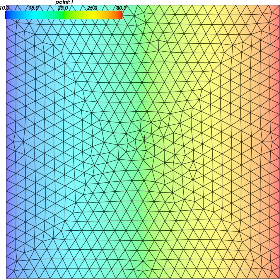
The paper’s principal example solves a coupled thermo‑elastic problem on a 2‑D square domain. First, a Laplace equation for temperature is solved with Dirichlet boundary conditions (10 °C on the left, 30 °C on the right) using a quadratic scalar field. The resulting temperature field is then used as a thermal load in a linear isotropic elasticity problem with Lamé parameters λ = 10, μ = 5, and thermal expansion coefficient α = 0.5. Displacements are constrained on the bottom (zero) and on the x‑component of the top edge (zero). The script explicitly creates Mesh, Domain, Regions, Fields, Variables, Materials, Terms, Equations, Boundary Conditions, and Solver objects, then solves the temperature problem, updates the temperature load, and solves the elasticity problem. Results are written to a VTK file and visualized with Mayavi (warped mesh, scalar field, wireframe).

An alternative “problem description file” (PDF) approach is also shown. In this mode, the user defines mesh, regions, fields, variables, materials, integrals, equations, and solvers using plain Python dictionaries and tuples. The same thermo‑elastic problem can be solved without writing any procedural code; the SfePy driver (simple.py) reads the PDF, constructs the objects automatically, and runs the simulation. This demonstrates SfePy’s dual nature as both a programmable library for custom applications and a black‑box solver for users who prefer configuration‑only workflows.

In conclusion, SfePy offers a flexible, Python‑centric environment for rapid prototyping and research‑level finite‑element simulations. Its term‑based abstraction, integration with the scientific Python stack, and support for multiple solver back‑ends make it attractive for a wide range of applications. Limitations include high memory usage for high‑order elements, lack of dedicated structural shells/plates/beams, and incomplete support for electromagnetics pending vector‑basis implementation. Addressing these issues will further broaden SfePy’s applicability across scientific and engineering domains.