CoSaMP: Iterative signal recovery from incomplete and inaccurate samples

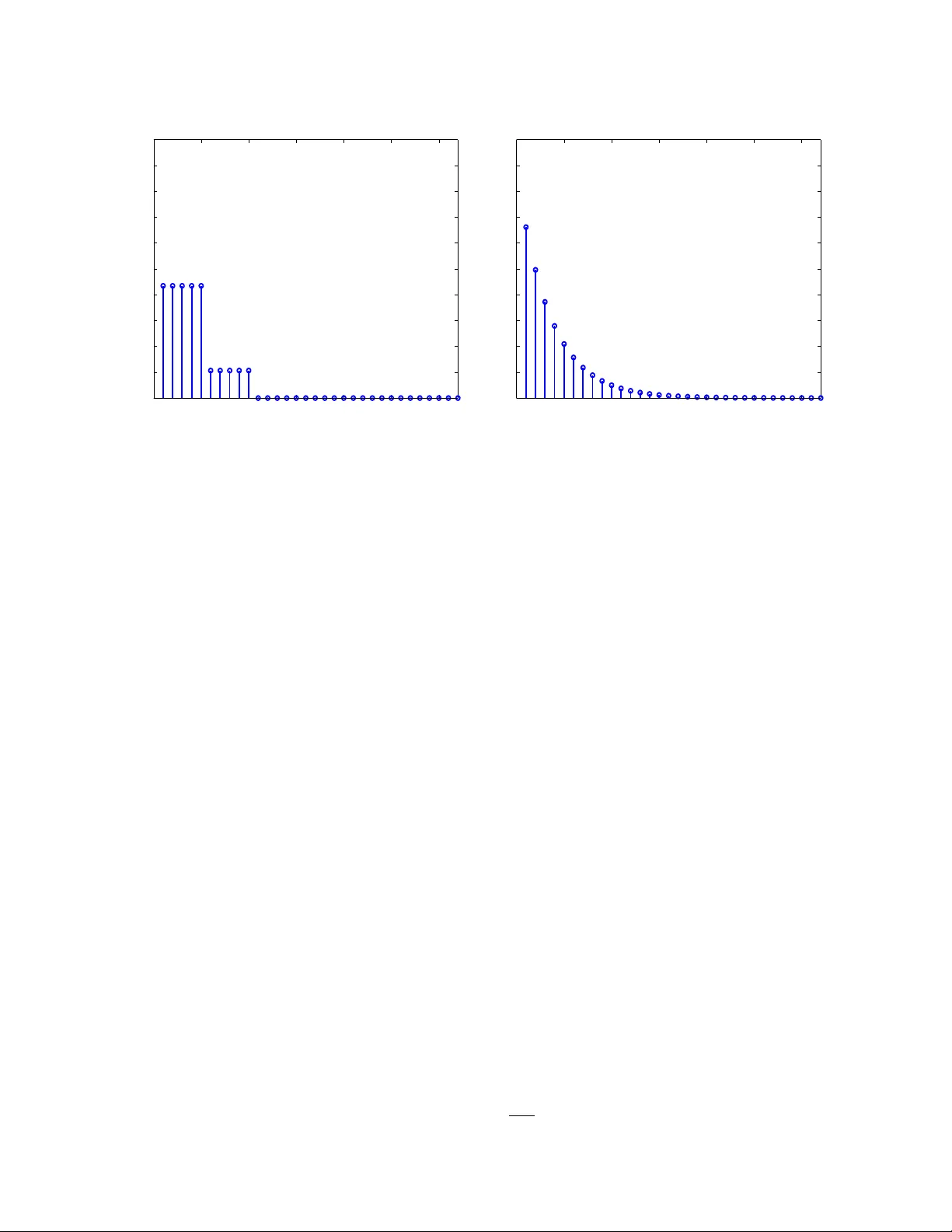
COSAMP: ITERA TIVE SIGNAL RECO VER Y FR OM INCOMPLETE AND INA CCURA TE SAMPLES D. NEEDELL AND J. A. TR OPP Abstract. Compressiv e sampling oﬀers a new paradigm for acquiring signals that are compressible with resp ect to an orthonormal basis. The ma jor algorithmic challeng e in compressive sampling is to appro ximate a compressible signal from noisy samples. This pap er describ es a new iterativ e reco very algorithm called CoSaMP that deliv ers the same guaran tees as the best optimization-based approac hes. Moreov er, this algorithm oﬀers rigorous b ounds on computational cost and storage. It is lik ely to b e extremely eﬃcient for practical problems b ecause it requires only matrix–v ector m ultiplies with the sampling matrix. F or compressible signals, the running time is just O( N log 2 N ), where N is the length of the signal. 1. Introduction Most signals of interest con tain scant information relative to their ambien t dimension, but the classical approach to signal acquisition ignores this fact. W e usually collect a complete represen- tation of the target signal and pro cess this represen tation to sieve out the actionable information. Then w e discard the rest. Con templating this ugly ineﬃciency , one might ask if it is p ossible instead to acquire c ompr essive samples . In other w ords, is there some t yp e of measuremen t that automatically winnows out the information from a signal? Incredibly , the answer is sometimes yes . Compr essive sampling refers to the idea that, for certain types of signals, a small n umber of nonadaptiv e samples carries suﬃcien t information to appro ximate the signal w ell. Research in this area has tw o ma jor comp onents: Sampling: How many samples are necessary to reconstruct signals to a sp eciﬁed precision? What t yp e of samples? Ho w can these sampling sc hemes b e implemen ted in practice? Reconstruction: Given the compressive samples, what algorithms can eﬃciently construct a signal approximation? The literature already con tains a w ell-dev elop ed theory of sampling, whic h we summarize b elo w. Although algorithmic work has b een progressing, the state of kno wledge is less than complete. W e assert that a practical signal reconstruction algorithm should hav e all of the following prop erties. • It should accept samples from a v ariety of sampling sc hemes. • It should succeed using a minimal num b er of samples. • It should b e robust when samples are con taminated with noise. • It should pro vide optimal error guarantees for every target signal. • It should oﬀer pro v ably eﬃcient resource usage. T o our kno wledge, no approach in the literature sim ultaneously accomplishes all ﬁve goals. Date : 16 March 2008. Revised 16 April 2008. Initially presented at Information Theory and Applications, 31 Jan uary 2008, San Diego. 2000 Mathematics Subje ct Classiﬁcation. 41A46, 68Q25, 68W20, 90C27. Key wor ds and phr ases. Algorithms, approximation, basis pursuit, compressed sensing, orthogonal matc hing pur- suit, restricted isometry property , signal reco very , sparse approximation, uncertain t y principle. DN is with the Mathematics Dept., Univ. California at Davis, 1 Shields Ave., Da vis, CA 95616. E-mail: dneedell@ math.ucdavis.edu . JA T is with Applied and Computational Mathematics, MC 217-50, California Inst. T echnology , P asadena, CA 91125. E-mail: jtropp@acm.caltech.edu . 1 2 D. NEEDELL AND J. A. TROPP This pap er presents and analyzes a nov el signal reconstruction algorithm that ac hiev es these desiderata. The algorithm is called CoSaMP , from the acrostic Compr essive Sampling Matching Pursuit . As the name suggests, the new metho d is ultimately based on orthogonal matc hing pursuit (OMP) [36], but it incorp orates several other ideas from the literature to accelerate the algorithm and to provide strong guaran tees that OMP cannot. Before w e describe the algorithm, let us deliver an in tro duction to the theory of compressiv e sampling. 1.1. Rudimen ts of Compressiv e Sampling. T o enhance intuition, w e focus on sparse and com- pressible signals. F or v ectors in C N , deﬁne the ` 0 quasi-norm k x k 0 = | supp( x ) | = |{ j : x j 6 = 0 }| . W e say that a signal x is s -sp arse when k x k 0 ≤ s . Sparse signals are an idealization that we do not encounter in applications, but real signals are quite often c ompr essible , which means that their en tries decay rapidly when sorted b y magnitude. As a result, compressible signals are w ell appro ximated by sparse signals. W e can also talk ab out signals that are compressible with resp ect to other orthonormal bases, suc h as a F ourier or w a velet basis. In this case, the sequence of co eﬃcien ts in the orthogonal expansion deca ys quickly . It represents no loss of generality to fo cus on signals that are compressible with resp ect to the standard basis, and we do so without regret. F or a more precise deﬁnition of compressibilit y , turn to Section 2.6. In the theory of compressiv e sampling, a sample is a linear functional applied to a signal. The pro cess of collecting m ultiple samples is b est viewed as the action of a sampling matrix Φ on the target signal. If we take m samples, or me asur ements , of a signal in C N , then the sampling matrix Φ has dimensions m × N . A natural question now arises: How many me asur ements ar e ne c essary to ac quir e s -sp arse signals? The minimum num b er of measuremen ts m ≥ 2 s on account of the follo wing simple argumen t. The sampling matrix m ust not map t w o diﬀerent s -sparse signals to the same set of samples. Therefore, each collection of 2 s columns from the sampling matrix m ust b e nonsingular. It is easy to see that certain V andermonde matrices satisfy this property , but these matrices are not really suitable for signal acquisition b ecause they con tain square minors that are very badly conditioned. As a result, some sparse signals are mapp ed to very similar sets of samples, and it is unstable to in v ert the sampling pro cess numerically . Instead, Cand` es and T ao prop osed the stronger condition that the geometry of sparse signals should b e preserv ed under the action of the sampling matrix [6]. T o quantify this idea, they deﬁned the r th r estricte d isometry c onstant of a matrix Φ as the least n um b er δ r for whic h (1 − δ r ) k x k 2 2 ≤ k Φ x k 2 2 ≤ (1 + δ r ) k x k 2 2 whenev er k x k 0 ≤ r . (1.1) W e ha ve written k·k 2 for the ` 2 v ector norm. When δ r < 1, these inequalities im ply that each collection of r columns from Φ is nonsingular, which is the minim um requirement for acquiring ( r / 2)-sparse signals. When δ r  1, the sampling op erator v ery nearly main tains the ` 2 distance b et ween each pair of ( r / 2)-sparse signals. In consequence, it is possible to in v ert the sampling pro cess stably . T o acquire s -sparse signals, one therefore hop es to achiev e a small restricted isometry constant δ 2 s with as few samples as p ossible. A striking fact is that man y t yp es of random matrices hav e excellen t restricted isometry b ehavior. F or example, w e can often obtain δ 2 s ≤ 0 . 1 with m = O( s log α N ) measuremen ts, where α is a small integer. Unfortunately , no deterministic sampling matrix is kno wn to satisfy a comparable b ound. Even worse, it is computationally diﬃcult to c hec k the inequalities (1.1), so it ma y never be p ossible to exhibit an explicit example of a goo d sampling matrix. COSAMP: ITERA TIVE SIGNAL RECO VER Y FROM NOISY SAMPLES 3 As a result, it is imp ortant to understand how random sampling matrices b ehav e. The t wo quin tessen tial examples are Gaussian matrices and partial F ourier matrices. Gaussian matrices: If the en tries of √ m Φ are indep endent and identically distributed stan- dard normal v ariables then m ≥ C r log ( N /r ) ε 2 = ⇒ δ r ≤ ε (1.2) except with probability e − c m . See [6] for details. P artial F ourier matrices: If √ m Φ is a uniformly random set of m ro ws dra wn from the N × N unitary discrete F ourier transform (DFT), then m ≥ C r log 5 N · log ( ε − 1 ) ε 2 = ⇒ δ r ≤ ε (1.3) except with probability N − 1 . See [32] for the pro of. Exp erts b eliev e that the p ow er on the ﬁrst logarithm should b e no greater than tw o [30]. Here and elsewhere, we follo w the analyst’s conv ention that upright letters (c , C , . . . ) refer to p ositiv e, univ ersal constan ts that may change from app earance to appearance. The Gaussian matrix is imp ortant b ecause it has optimal restricted isometry b ehavior. Indeed, for an y m × N matrix, δ r ≤ 0 . 1 = ⇒ m ≥ C r log( N /r ) , on accoun t of profound geometric results of Kashin [23] and Garnaev–Gluskin [15]. Even though partial F ourier matrices may require additional samples to achiev e a small restricted isometry constan t, they are more interesting for the following reasons [2]. • There are technologies that acquire random F ourier measurements at unit cost p er sample. • The sampling matrix can b e applied to a v ector in time O( N log N ). • The sampling matrix requires only O( m log N ) storage. Other types of sampling matrices, suc h as the r andom demo dulator [35], enjo y similar qualities. These traits are essential for the translation of compressive sampling from theory into practice. 1.2. Signal Recov ery Algorithms. The ma jor algorithmic c hallenge in compressive sampling is to appro ximate a signal given a vector of noisy samples. The literature describ es a huge num b er of approac hes to solving this problem. They fall in to three rough categories: Greedy pursuits: These metho ds build up an approximation one step at a time by mak- ing lo cally optimal c hoices at eac h step. Examples include OMP [36], stagewise OMP (StOMP) [13], and regularized OMP (R OMP) [28, 27]. Con v ex relaxation: These tec hniques solve a conv ex program whose minimizer is known to approximate the target signal. Many algorithms ha ve been prop osed to complete the optimization, including interior-point methods [2, 24], pro jected gradien t methods [14], and iterativ e thresholding [11]. Com binatorial algorithms: These metho ds acquire highly structured samples of the sig- nal that support rapid reconstruction via group testing. This class includes F ourier sam- pling [19, 21], c haining pursuit [16], and HHS pursuit [17], as w ell as some algorithms of Cormo de–Muth ukrishnan [9] and Iwen [22]. A t present, each t yp e of algorithm has its native shortcomings. Man y of the combinatorial algorithms are extremely fast—sublinear in the length of the target signal—but they require a large num b er of somewhat un usual samples that may not b e easy to acquire. A t the other extreme, con v ex relaxation algorithms succeed with a v ery small n um ber of measurements, but they tend to b e computationally burdensome. Greedy pursuits—in particular, the R OMP algorithm—are in termediate in their running time and sampling eﬃciency . 4 D. NEEDELL AND J. A. TROPP CoSaMP , the algorithm describ ed in this paper, is at heart a greedy pursuit. It also incorp orates ideas from the com binatorial algorithms to guaran tee sp eed and to pro vide rigorous error b ounds [17]. The analysis is inspired by the w ork on R OMP [28, 27] and the w ork of Cand` es–Rom b erg–T ao [3] on conv ex relaxation metho ds. In particular, we establish the following result. Theorem A ( CoSaMP ) . Supp ose that Φ is an m × N sampling matrix with r estricte d isometry c onstant δ 2 s ≤ c . L et u = Φ x + e b e a ve ctor of samples of an arbitr ary signal, c ontaminate d with arbitr ary noise. F or a given pr e cision p ar ameter η , the algorithm CoSaMP pr o duc es a 2 s -sp arse appr oximation a that satisﬁes k x − a k 2 ≤ C · max  η , 1 √ s k x − x s k 1 + k e k 2  wher e x s is a b est s -sp arse appr oximation to x . The running time is O( L · log ( k x k 2 /η )) , wher e L b ounds the c ost of a matrix–ve ctor multiply with Φ or Φ ∗ . The working stor age use is O( N ) . Let us expand on the statement of this result. First, recall that many types of random sampling matrices satisfy the restricted isometry hypothesis when the num ber of samples m = O( s log α N ). Therefore, the theorem applies to a wide class of sampling schemes when the n umber of samples is prop ortional to the target sparsity and logarithmic in the am bient dimension of the signal space. The algorithm pro duces a 2 s -sparse appro ximation whose ` 2 error is comparable with the scaled ` 1 error of the b est s -sparse approximation to the signal. Of course, the algorithm cannot resolv e the uncertain ty due to the additiv e noise, so w e also pay for the energy in the noise. This type of error bound is structurally optimal, as w e discuss in Section 2.6. Some disparit y in the sparsity lev els (here, 2 s v ersus s ) seems to be necessary when the reco very algorithm is computationally eﬃcien t [31]. W e can interpret the error guarantee as follows. In the absence of noise, the algorithm can reco v er an s -sparse signal to arbitrarily high precision. Performance degrades gracefully as the energy in the noise increases. Performance also degrades gracefully for compressible signals. The theorem is ultimately v acuous for signals that cannot b e appro ximated by sparse signals, but compressive sampling is not an appropriate tec hnique for this class. The running time b ound indicates that each matrix–vector multiplication reduces the error by a constant factor (if w e amortize o v er the entire execution). That is, the algorithm has linear con v ergence 1 . W e ﬁnd that the total run time is roughly prop ortional to (the negation of ) the r e c onstruction signal-to-noise r atio R-SNR = 10 log 10  k x − a k 2 k x k 2  dB . F or compressible signals, one can show that | R-SNR | = O(log s ). The runtime is also prop ortional to the cost of a matrix–vector multiply . F or sampling matrices with a fast m ultiply , the algorithm is accelerated substantially . In particular, for the partial F ourier matrix, a matrix–vector multiply requires time O( N log N ). It follows that the total runtime is O( N log N · | R-SNR | ). F or most signals of interest, this cost is nearly linear in the signal length! 1.3. Notation. Let us instate sev eral pieces of notation that are carried throughout the paper. F or p ∈ [1 , ∞ ], w e write k·k p for the usual ` p v ector norm. W e reserve the symbol k·k for the sp ectral norm, i.e., the natural norm on linear maps from ` 2 to ` 2 . Supp ose that x is a signal in C N and r is a positive in teger. W e write x r for the signal in C N that is formed b y restricting x to its r largest-magnitude comp onents. Ties are brok en lexicographically . 1 Mathematicians sometimes refer to linear conv ergence as “exp onential conv ergence.” COSAMP: ITERA TIVE SIGNAL RECO VER Y FROM NOISY SAMPLES 5 This signal is a b est r -sparse approximation to x with resp ect to an y ` p norm. Supp ose now that T is a subset of { 1 , 2 , . . . , N } . W e deﬁne the restriction of the signal to the set T as x | T = ( x i , i ∈ T 0 , otherwise . W e o ccasionally abuse the notation and treat x | T as an element of the v ector space C T . W e also deﬁne the restriction Φ T of the sampling matrix Φ as the column submatrix whose columns are listed in the set T . Finally , w e deﬁne the pseudoinv erse of a tall, full-rank matrix A by the form ula A † = ( A ∗ A ) − 1 A ∗ . 1.4. Organization. The rest of the pap er has the follo wing structure. In Section 2 we introduce the CoSaMP algorithm, w e state the ma jor theorems in more detail, and w e discuss implemen tation and resource requirements. Section 3 describ es some consequences of the restricted isometry prop erty that p erv ade our analysis. The central theorem is established for sparse signals in Sections 4 and 5. W e extend this result to general signals in Section 6. Finally , Section 7 places the algorithm in the con text of previous work. The ﬁrst appendix presen ts v ariations on the algorithm. The second app endix con tains a b ound on the n umber of iterations required when the algorithm is implemented using exact arithmetic. 2. The CoSaMP Algorithm This section gives an o v erview of the algorithm, along with explicit pseudo co de. It presents the ma jor theorems on the p erformance of the algorithm. Then it co v ers details of implemen tation and b ounds on resource requirements. 2.1. In tuition. The most diﬃcult part of signal reconstruction is to iden tify the lo cations of the largest comp onents in the target signal. CoSaMP uses an approac h inspired b y the restricted isometry prop erty . Supp ose that the sampling matrix Φ has restricted isometry constant δ s  1. F or an s -sparse signal x , the v ector y = Φ ∗ Φ x can serve as a pro xy for the signal b ecause the energy in each set of s comp onents of y approximates the energy in the corresponding s comp onents of x . In particular, the largest s en tries of the pro xy y p oint tow ard the largest s en tries of the signal x . Since the samples hav e the form u = Φ x , we can obtain the proxy just b y applying the matrix Φ ∗ to the samples. The algorithm in v okes this idea iteratively to approximate the target signal. At eac h iteration, the current appro ximation induces a residual, the part of the target signal that has not b een appro ximated. As the algorithm progresses, the samples are up dated so that they reﬂect the curren t residual. These samples are used to construct a proxy for the residual, whic h p ermits us to identify the large comp onents in the residual. This step yields a tentativ e supp ort for the next appro ximation. W e use the samples to estimate the appro ximation on this supp ort set using least squares. This pro cess is rep eated un til we hav e found the reco verable energy in the signal. 2.2. Ov erview. As input, the CoSaMP algorithm requires four pieces of information: • Access to the sampling op erator via matrix–vector multiplication. • A vector of (noisy) samples of the unkno wn signal. • The sparsity of the appro ximation to b e pro duced. • A halting criterion. The algorithm is initialized with a trivial signal appro ximation, whic h means that the initial residual equals the unknown target signal. During eac h iteration, CoSaMP p erforms ﬁve ma jor steps: (1) Identiﬁcation. The algorithm forms a proxy of the residual from the current samples and lo cates the largest comp onents of the pro xy . 6 D. NEEDELL AND J. A. TROPP (2) Supp ort Merger. The set of newly iden tiﬁed comp onents is united with the set of com- p onen ts that appear in the curren t appro ximation. (3) Estimation. The algorithm solv es a least-squares problem to appro ximate the target signal on the merged set of comp onen ts. (4) Pruning. The algorithm pro duces a new approximation by retaining only the largest en tries in this least-squares signal appro ximation. (5) Sample Up date. Finally , the samples are up dated so that they reﬂect the residual, the part of the signal that has not b een approximated. These steps are rep eated un til the halting criterion is triggered. In the b o dy of this w ork, we concen trate on methods that use a ﬁxed n um ber of iterations. App endix A discusses some other simple stopping rules that ma y also be useful in practice. Pseudo co de for CoSaMP app ears as Algorithm 2.1. This co de describ es the version of the al- gorithm that we analyze in this pap er. Nevertheless, there are sev eral adjustable parameters that ma y improv e p erformance: the n um ber of comp onents selected in the identiﬁcation step and the n um b er of comp onents retained in the pruning step. F or a brief discussion of other v ariations on the algorithm, turn to App endix A. Algorithm 2.1: CoSaMP Recov ery Algorithm CoSaMP ( Φ , u , s ) Input: Sampling matrix Φ , noisy sample vector u , sparsit y lev el s Output: An s -sparse appro ximation a of the target signal a 0 ← 0 { T rivial initial approximation } v ← u { Curren t samples = input samples } k ← 0 rep eat k ← k + 1 y ← Φ ∗ v { F orm signal proxy } Ω ← supp( y 2 s ) { Iden tify large comp onents } T ← Ω ∪ supp( a k − 1 ) { Merge supp orts } b | T ← Φ † T u { Signal estimation by least-squares } b | T c ← 0 a k ← b s { Prune to obtain next appro ximation } v ← u − Φ a k { Update current samples } un til halting criterion true COSAMP: ITERA TIVE SIGNAL RECO VER Y FROM NOISY SAMPLES 7 2.3. P erformance Guaran tees. This section describ es our theoretical analysis of the b eha vior of CoSaMP . The next section cov ers the resource requirements of the algorithm. Afterw ard, Section 2.5 com bines these materials to establish Theorem A. Our results dep end on a set of h yp otheses that has b ecome common in the compressive sampling literature. Let us frame the standing assumptions: CoSaMP Hypotheses • The sparsity level s is ﬁxed. • The m × N sampling op erator Φ has restricted isometry constant δ 4 s ≤ 0 . 1. • The signal x ∈ C N is arbitrary , except where noted. • The noise v ector e ∈ C m is arbitrary . • The vector of samples u = Φ x + e . W e also deﬁne the unr e c over able ener gy ν in the signal. This quantit y measures the baseline error in our approximation that o ccurs b ecause of noise in the samples or b ecause the signal is not sparse. ν = k x − x s k 2 + 1 √ s k x − x s k 1 + k e k 2 . (2.1) W e p ostp one a more detailed discussion of the unreco v erable energy until Section 2.6. Our k ey result is that CoSaMP mak es signiﬁcant progress during eac h iteration where the ap- pro ximation error is large relative to the unrecov erable energy . Theorem 2.1 (Iteration Inv ariant) . F or e ach iter ation k ≥ 0 , the signal appr oximation a k is s -sp arse and   x − a k +1   2 ≤ 0 . 5   x − a k   2 + 10 ν . In p articular,   x − a k   2 ≤ 2 − k k x k 2 + 20 ν . The pro of of Theorem 2.1 will o ccup y us for most of this pap er. In Section 4, we establish an analog for sparse signals. The version for general signals app ears as a corollary in Section 6. Theorem 2.1 has some immediate consequences for the qualit y of reconstruction with resp ect to standard signal metrics. In this setting, a sensible deﬁnition of the signal-to-noise r atio (SNR) is SNR = 10 log 10  k x k 2 ν  . The r e c onstruction SNR is deﬁned as R-SNR = 10 log 10  k x − a k 2 k x k 2  . Both quantities are measured in decib els. Theorem 2.1 implies that, after k iterations, the recon- struction SNR satisﬁes R-SNR > 3 − min { 3 k , SNR − 13 } . In words, eac h iteration reduces the reconstruction SNR b y ab out 3 decib els until the error nears the noise ﬂo or. T o reduce the error to its minimal v alue, the num b er of iterations is prop ortional to the SNR. Let us consider a slightly diﬀeren t scenario. Suppose that the signal x is s -sparse, so the unre- co v erable energy ν = k e k 2 . Deﬁne the dynamic r ange ∆ = 10 log 10  max | x i | min | x i |  where i ranges ov er supp( x ). 8 D. NEEDELL AND J. A. TROPP Assume moreov er that the minimum nonzero comp onen t of the signal is at least 40 ν . Using the fact that k x k 2 ≤ √ s k x k ∞ , it is easy to chec k that k x − a k 2 ≤ min | x i | as so on as the num b er k of iterations satisﬁes k ? 3 . 3∆ + log 2 √ s + 1 . It follo ws that the supp ort of the appro ximation a must contain every entry in the supp ort of the signal x . This discussion suggests that the num ber of iterations migh t b e substan tial if w e require a very lo w reconstruction SNR or if the signal has a very wide dynamic range. This initial impression is not en tirely accurate. W e ha ve established that, when the algorithm p erforms arithmetic to high enough precision, then a ﬁxed num ber of iterations suﬃces to reduce the approximation error to the same order as the unreco v erable energy . Here is a result for exact computations. Theorem 2.2 (Iteration Count) . Supp ose that CoSaMP is implemente d with exact arithmetic. After at most 6( s + 1) iter ations, CoSaMP pr o duc es an s -sp arse appr oximation a that satisﬁes k x − a k 2 ≤ 20 ν . In fact, ev en more is true. The num ber of iterations depends signiﬁcantly on the structure of the signal. The only situation where the algorithm needs Ω( s ) iterations o ccurs when the entries of the signal deca y exp onen tially . F or signals whose largest entries are comparable, the num ber of iterations ma y be as small as O(log s ). This claim is quantiﬁed in App endix B, where we prov e Theorem 2.2. If we solv e the least-squares problems to high precision, an analogous result holds, but the appro ximation guarantee contains an extra term that comes from solving the least-squares problems imp erfectly . In practice, it may b e more eﬃcient ov erall to solve the least-squares problems to lo w precision. The correct amoun t of care seems to dep end on the relative costs of forming the signal pro xy and solving the least-squares problem, which are the t wo most exp ensiv e steps in the algorithm. W e discuss this p oint in the next section. Ultimately , the question is b est settled with empirical studies. Remark 2.3. In the hyp otheses, a b ound on the r estricte d isometry c onstant δ 2 s also suﬃc es. Inde e d, Cor ol lary 3.4 of the se quel implies that δ 4 s ≤ 0 . 1 holds whenever δ 2 s ≤ 0 . 025 . Remark 2.4. The expr ession (2.1) for the unr e c over able ener gy c an b e simpliﬁe d using L emma 7 fr om [17] , which states that, for every signal y ∈ C N and every p ositive inte ger t , we have k y − y t k 2 ≤ 1 2 √ t k y k 1 . Cho osing y = x − x s/ 2 and t = s/ 2 , we r e ach ν ≤ 1 . 71 √ s   x − x s/ 2   1 + k e k 2 . (2.2) In wor ds, the unr e c over able ener gy is c ontr ol le d by the sc ale d ` 1 norm of the signal tail. 2.4. Implemen tation and Resource Requiremen ts. CoSaMP was designed to b e a practical metho d for signal reco v ery . An eﬃcient implemen tation of the algorithm requires some ideas from n umerical linear algebra, as w ell as some basic tec hniques from the theory of algorithms. This section discusses the k ey issues and dev elops an analysis of the running time for the tw o most common scenarios. W e fo cus on the least-squares problem in the estimation step because it is the ma jor obstacle to a fast implemen tation of the algorithm. The algorithm guaran tees that the matrix Φ T nev er has more than 3 s columns, so our assumption δ 4 s ≤ 0 . 1 implies that the matrix Φ T is extremely w ell conditioned. As a result, w e can apply the pseudoin v erse Φ † T = ( Φ ∗ T Φ T ) − 1 Φ ∗ T v ery quic kly using an iterativ e metho d, suc h as Ric hardson’s iteration [1, Sec. 7.2.3] or conjugate gradien t [1, COSAMP: ITERA TIVE SIGNAL RECO VER Y FROM NOISY SAMPLES 9 Sec. 7.4]. These techniques hav e the additional adv an tage that they only interact with the matrix Φ T through its action on vectors. It follo ws that the algorithm p erforms b etter when the sampling matrix has a fast matrix–v ector m ultiply . Section 5 con tains an analysis of the p erformance of iterativ e least-squares algorithms in the con text of CoSaMP . In summary , if we initialize the least-squares metho d with the current approx- imation a k − 1 , then the cost of solving the least-squares problem is O( L ), where L bounds the cost of a matrix–v ector m ultiply with Φ T or Φ ∗ T . This implementation ensures that Theorem 2.1 holds at each iteration. W e emphasize that direct methods for least squares are lik ely to be extremely ineﬃcient in this setting. The ﬁrst reason is that eac h least-squares problem may contain substan tially diﬀeren t sets of columns from Φ . As a result, it b ecomes necessary to p erform a completely new QR or SVD factorization during eac h iteration at a cost of O( s 2 m ). The second problem is that computing these factorizations t ypically requires direct access to the columns of the matrix, whic h is problematic when the matrix is accessed through its action on v ectors. Third, direct metho ds hav e storage costs O( sm ), whic h may b e deadly for large-scale problems. The remaining steps of the algorithm are standard. Let us estimate the op eration coun ts. Pro xy: F orming the proxy is dominated b y the cost of the matrix–v ector m ultiply Φ ∗ v . Iden tiﬁcation: W e can lo cate the largest 2 s entries of a v ector in time O( N ) using the approac h in [8, Ch. 9]. In practice, it may b e faster to sort the entries of the signal in decreasing order of magnitude at cost O( N log N ) and then select the ﬁrst 2 s of them. The latter pro cedure can b e accomplished with quicksort, mergesort, or heapsort [8, Sec. I I]. T o implemen t the algorithm to the letter, the sorting metho d needs to b e stable b ecause w e stipulate that ties are brok en lexicographically . This p oint is not imp ortan t in practice. Supp ort Merger: W e can merge t w o sets of size O( s ) in exp ected time O( s ) using random- ized hashing metho ds [8, Ch. 11]. One can also sort b oth sets ﬁrst and use the elemen tary merge procedure [8, p. 29] for a total cost O( s log s ). LS estimation: W e use Richardson’s iteration or conjugate gradien t to compute Φ † T u . Ini- tializing the least-squares algorithm requires a matrix–v ector m ultiply with Φ ∗ T . Eac h iteration of the least-squares metho d requires one matrix–v ector mu ltiply each with Φ T and Φ ∗ T . Since Φ T is a submatrix of Φ , the matrix–v ector multiplies can also b e obtained from m ultiplication with the full matrix. W e prov e in Section 5 that a constan t n umber of least-squares iterations suﬃces for Theorem 2.1 to hold. Pruning: This step is similar to identiﬁcation. Pruning can b e implemen ted in time O( s ), but it may b e preferable to sort the comp onents of the vector b y magnitude and then select the ﬁrst s at a cost of O( s log s ). Sample Up date: This step is dominated by the cost of the m ultiplication of Φ with the s -sparse v ector a k . T able 1 summarizes this discussion in tw o particular cases. The ﬁrst column sho ws what happ ens when the sampling matrix Φ is applied to vectors in the standard wa y , but we hav e random access to submatrices. The second, column shows what happ ens when the sampling matrix Φ and its adjoin t Φ ∗ b oth hav e a fast multiply with cost L , where w e assume that L ≥ N . A t ypical v alue is L = O( N log N ). In particular, a partial F ourier matrix satisﬁes this b ound. Finally , w e note that the storage requiremen ts of the algorithm are also fav orable. Aside from the storage required b y the sampling matrix, the algorithm constructs only one vector of length N , the signal pro xy . The sample v ectors u and v hav e length m , so they require O( m ) storage. The signal appro ximations can be stored using sparse data structures, so they require at most O( s log N ) storage. Similarly , the index sets that app ear require only O( s log N ) storage. The total storage is O( N ). 10 D. NEEDELL AND J. A. TROPP T able 1. Op eration count for CoSaMP . Big-O notation is omitted for legibility . The dimensions of the sampling matrix Φ are m × N ; the sparsity level is s . The n um b er L b ounds the cost of a matrix–v ector m ultiply with Φ or Φ ∗ . Step Standard m ultiply F ast multiply F orm pro xy mN L Iden tiﬁcation N N Supp ort merger s s LS estimation sm L Pruning s s Sample update sm L T otal p er iteration O( mN ) O( L ) The follo wing result summarizes this discussion. Theorem 2.5 (Resource Requiremen ts) . Each iter ation of CoSaMP r e quir es O( L ) time, wher e L b ounds the c ost of a multiplic ation with the matrix Φ or Φ ∗ . The algorithm uses stor age O( N ) . Remark 2.6. We have b e en able to show that The or em 2.2 holds when the le ast-squar es pr ob- lems ar e solve d iter atively with a delic ately chosen stopping thr eshold. In this c ase, the total numb er of le ast-squar es iter ations p erforme d over the entir e exe cution of the algorithm is at most O(log( k x k 2 /η )) if we wish to achieve err or O( η + ν ) . When the c ost of forming the signal pr oxy is much higher than the c ost of solving the le ast-squar es pr oblem, this analysis may yield a sharp er r esult. F or example, using standar d matrix–ve ctor multiplic ation, we have a runtime b ound O( s · mN + log ( k x k 2 /η ) · sm ) . The ﬁrst term r eﬂe cts the numb er of CoSaMP iter ations times the c ost of forming the signal pr oxy. The se c ond term r eﬂe cts the total c ost of the le ast-squar es iter ations. Unless the r elative pr e cision k x k 2 /η is sup er exp onential in the signal length, we obtain running time O( smN ) . This b ound is c omp ar able with the worst-c ase c ost of OMP or R OMP. As we discuss in App endix B, the numb er of CoSaMP iter ations may b e much smal ler than s , which also impr oves the estimate. 2.5. Pro of of Theorem A. W e ha v e no w collected all the material we need to establish the main result. Fix a precision parameter η . After at most O(log( k x k 2 /η )) iterations, CoSaMP pro duces an s -sparse approximation a that satisﬁes k x − a k 2 ≤ C · ( η + ν ) in consequence of Theorem 2.1. Apply inequalit y (2.2) to b ound the unrecov erable energy ν in terms of the ` 1 norm. W e see that the approximation error satisﬁes k x − a k 2 ≤ C · max  η , 1 √ s   x − x s/ 2   1 + k e k 2  . According to Theorem 2.5, each iteration of CoSaMP is completed in time O( L ), where L b ounds the cost of a matrix–vector multiplication with Φ or Φ ∗ . The total runtime, therefore, is O( L log ( k x k 2 /η )). The total storage is O( N ). In the statemen t of the theorem, p erform the substitution s/ 2 7→ s . Finally , we replace δ 8 s with δ 2 s b y means of Corollary 3.4, whic h states that δ cr ≤ c · δ 2 r for an y p ositiv e in tegers c and r . COSAMP: ITERA TIVE SIGNAL RECO VER Y FROM NOISY SAMPLES 11 2.6. The Unreco v erable Energy. Since the unrecov erable energy ν plays a central role in our analysis of CoSaMP , it merits some additional discussion. In particular, it is informativ e to examine the unreco v erable energy in a compressible signal. Let p b e a num b er in the interv al (0 , 1). W e say that x is p -c ompr essible with magnitude R if the sorted comp onents of the signal decay at the rate | x | ( i ) ≤ R · i − 1 /p for i = 1 , 2 , 3 , . . . . When p = 1, this deﬁnition implies that k x k 1 ≤ R · (1 + log N ). Therefore, the unit ball of 1-compressible signals is similar to the ` 1 unit ball. When p ≈ 0, this deﬁnition implies that p - compressible signals are very nearly sparse. In general, compressible signals are w ell approximated b y sparse signals: k x − x s k 1 ≤ C p · R · s 1 − 1 /p k x − x s k 2 ≤ D p · R · s 1 / 2 − 1 /p where C p = (1 /p − 1) − 1 and D p = (2 /p − 1) − 1 / 2 . These results follo w b y writing eac h norm as a sum and appro ximating the sum with an in tegral. W e see that the unreco verable energy (2.1) in a p -compressible signal is b ounded as ν ≤ 2C p · R · s 1 / 2 − 1 /p + k e k 2 . (2.3) When p is small, the ﬁrst term in the unrecov erable energy deca ys rapidly as the sparsity level s increases. F or the class of p -compressible signals, the b ound (2.3) on the unreco v erable energy is sharp, modulo the exact v alues of the constan ts. With these inequalities, we can see that CoSaMP reco v ers compressible signals eﬃciently . Let us calculate the n um b er of iterations required to reduce the approximation error from k x k 2 to the optimal lev el (2.3). F or compressible signals, the energy k x k 2 ≤ 2 R , so log  2 R 2C p · R · s 1 / 2 − 1 /p  = log(1 /p − 1) + (1 /p − 1 / 2) log s. Therefore, the n um b er of iterations required to recov er a generic p -compressible signal is O(log s ), where the constant in the big-O notation dep ends on p . The term “unrecov erable energy” is justiﬁed by several facts. First, we must pay for the ` 2 error con taminating the samples. T o c hec k this p oint, deﬁne S = supp( x s ). The matrix Φ S is nearly an isometry from ` S 2 to ` m 2 , so an error in the large comp onen ts of the signal induces an error of equiv alent size in the samples. Clearly , w e can never resolve this uncertain ty . The term s − 1 / 2 k x − x s k 1 is also required on account of classical results ab out the Gel’fand widths of the ` N 1 ball in ` N 2 , due to Kashin [23] and Garnaev–Gluskin [15]. In the language of compressive sampling, their w ork has the following interpretation. Let Φ be a ﬁxed m × N sampling matrix. Supp ose that, for every signal x ∈ C N , there is an algorithm that uses the samples u = Φ x to construct an approximation a that ac hiev es the e rror b ound k x − a k 2 ≤ C √ s k x k 1 . Then the num ber m of measuremen ts m ust satisfy m ≥ c s log ( N /s ). 3. Restricted Isometr y Consequences When the sampling matrix satisﬁes the restricted isometry inequalities (1.1), it has sev eral other prop erties that w e require rep eatedly in the pro of that the CoSaMP algorithm is correct. Our ﬁrst observ ation is a simple translation of (1.1) into other terms. 12 D. NEEDELL AND J. A. TROPP Prop osition 3.1. Supp ose Φ has r estricte d isometry c onstant δ r . L et T b e a set of r indic es or fewer. Then   Φ ∗ T u   2 ≤ p 1 + δ r k u k 2   Φ † T u   2 ≤ 1 √ 1 − δ r k u k 2   Φ ∗ T Φ T x   2 S (1 ± δ r ) k x k 2   ( Φ ∗ T Φ T ) − 1 x   2 S 1 1 ± δ r k x k 2 . wher e the last two statements c ontain an upp er and lower b ound, dep ending on the sign chosen. Pr o of. The restricted isometry inequalities (1.1) imply that the singular v alues of Φ T lie b etw een √ 1 − δ r and √ 1 + δ r . The b ounds follow from standard relationships b etw een the singular v alues of Φ T and the singular v alues of basic functions of Φ T .  A second consequence is that disjoint sets of columns from the sampling matrix span nearly orthogonal subspaces. The following result quantiﬁes this observ ation. Prop osition 3.2 (Approximate Orthogonalit y) . Supp ose Φ has r estricte d isometry c onstant δ r . L et S and T b e disjoint sets of indic es whose c ombine d c ar dinality do es not exc e e d r . Then k Φ ∗ S Φ T k ≤ δ r . Pr o of. Abbreviate R = S ∪ T , and observ e that Φ ∗ S Φ T is a submatrix of Φ ∗ R Φ R − I . The sp ectral norm of a submatrix nev er exceeds the norm of the en tire matrix. W e discern that k Φ ∗ S Φ T k ≤ k Φ ∗ R Φ R − I k ≤ max { (1 + δ r ) − 1 , 1 − (1 − δ r ) } = δ r b ecause the eigenv alues of Φ ∗ R Φ R lie betw een 1 − δ r and 1 + δ r .  This result will b e applied through the following corollary . Corollary 3.3. Supp ose Φ has r estricte d isometry c onstant δ r . L et T b e a set of indic es, and let x b e a ve ctor. Pr ovide d that r ≥ | T ∪ supp( x ) | , k Φ ∗ T Φ · x | T c k 2 ≤ δ r k x | T c k 2 . Pr o of. Deﬁne S = supp( x ) \ T , so we hav e x | S = x | T c . Thus, k Φ ∗ T Φ · x | T c k 2 = k Φ ∗ T Φ · x | S k 2 ≤ k Φ ∗ T Φ S k k x | S k 2 ≤ δ r k x | T c k 2 , o wing to Prop osition 3.2.  As a second corollary , we sho w that δ 2 r giv es weak control o v er the higher restricted isometry constan ts. Corollary 3.4. L et c and r b e p ositive inte gers. Then δ cr ≤ c · δ 2 r . Pr o of. The result is clearly true for c = 1 , 2 , so we assume c ≥ 3. Let S b e an arbitrary index set of size cr , and let M = Φ ∗ S Φ S − I . It suﬃces to c hec k that k M k ≤ c · δ 2 r . T o that end, we break the matrix M into r × r blo c ks, whic h w e denote M ij . A block version of Gershgorin’s theorem states that k M k satisﬁes at least one of the inequalities |k M k − k M ii k| ≤ X j 6 = i k M ij k where i = 1 , 2 , . . . , c . The deriv ation is en tirely analogous with the usual pro of of Gershgorin’s theorem, so we omit the details. F or each diagonal block, w e ha v e k M ii k ≤ δ r b ecause of the restricted isometry inequalities (1.1). F or each oﬀ-diagonal block, we ha v e k M ij k ≤ δ 2 r b ecause of Prop osition 3.2. Substitute these bounds into the blo ck Gershgorin theorem and rearrange to complete the pro of.  COSAMP: ITERA TIVE SIGNAL RECO VER Y FROM NOISY SAMPLES 13 Finally , we presen t a result that measures ho w muc h the sampling matrix inﬂates nonsparse v ectors. This b ound p ermits us to establish the ma jor results for sparse signals and then transfer the conclusions to the general case. Prop osition 3.5 (Energy Bound) . Supp ose that Φ veriﬁes the upp er ine quality of (1.1) , viz. k Φ x k 2 ≤ p 1 + δ r k x k 2 when k x k 0 ≤ r. Then, for every signal x , k Φ x k 2 ≤ p 1 + δ r  k x k 2 + 1 √ r k x k 1  . Pr o of. W e rep eat the geometric argument of Rudelson that is presented in [17]. First, observe that the hypothesis of the prop osition can b e regarded as a statement ab out the op erator norm of Φ as a map b et w een tw o Banach spaces. F or a set I ⊂ { 1 , 2 , . . . , N } , write B I 2 for the unit ball in ` 2 ( I ). Deﬁne the conv ex b o dy S = con v  [ | I |≤ r B I 2  ⊂ C N , and notice that, by hy p othesis, the op erator norm k Φ k S → 2 = max x ∈ S k Φ x k 2 ≤ p 1 + δ r . Deﬁne a second conv ex b o dy K =  x : k x k 2 + 1 √ r k x k 1 ≤ 1  ⊂ C N , and consider the op erator norm k Φ k K → 2 = max x ∈ K k Φ x k 2 . The con ten t of the prop osition is the claim that k Φ k K → 2 ≤ k Φ k S → 2 . T o establish this p oin t, it suﬃces to chec k that K ⊂ S . Instead, we prov e the reverse inclusion for the p olars: S ◦ ⊂ K ◦ . The norm with unit ball S ◦ is calculated as k u k S ◦ = max | I |≤ r k u | I k 2 . Consider a vector u in the unit ball S ◦ , and let I b e a set of r co ordinates where u is largest in magnitude. W e must hav e k u | I c k ∞ ≤ 1 √ r , or else | u i | > 1 √ r for each i ∈ I . But then k u k S ◦ ≥ k u | I k 2 > 1, a contradiction. Therefore, we ma y write u = u | I + u | I c ∈ B 2 + 1 √ r B ∞ , where B p is the unit ball in ` N p . But the set on the righ t-hand side is precisely the unit ball of K ◦ since sup v ∈ K ◦ h x , v i = k x k K = k x k 2 + 1 √ r k x k 1 = sup v ∈ B 2 h x , v i + sup w ∈ 1 √ r B ∞ h x , w i = sup v ∈ B 2 + 1 √ r B ∞ h x , v i . In summary , S ◦ ⊂ K ◦ .  14 D. NEEDELL AND J. A. TROPP 4. The Itera tion Inv ariant: Sp arse Case W e now commence the pro of of Theorem 2.1. F or the momen t, let us assume that the signal is actually sparse. Section 6 remov es this assumption. The result states that eac h iteration of the algorithm reduces the appro ximation error by a con- stan t factor, while adding a small multiple of the noise. As a consequence, when the appro ximation error is large in comparison with the noise, the algorithm makes substan tial progress in iden tifying the unkno wn signal. Theorem 4.1 (Iteration Inv ariant: Sparse Case) . Assume that x is s -sp arse. F or e ach k ≥ 0 , the signal appr oximation a k is s -sp arse, and   x − a k +1   2 ≤ 0 . 5   x − a k   2 + 7 . 5 k e k 2 . In p articular,   x − a k   2 ≤ 2 − k k x k 2 + 15 k e k 2 . The argumen t pro ceeds in a sequence of short lemmas, each corresp onding to one step in the algorithm. Throughout this section, we retain the assumption that x is s -sparse. 4.1. Appro ximations, Residuals, etc. Fix an iteration k ≥ 1. W e write a = a k − 1 for the signal appro ximation at the b eginning of the iteration. Deﬁne the residual r = x − a , which w e interpret as the part of the signal w e ha v e not y et recov ered. Since the approximation a is alwa ys s -sparse, the residual r m ust b e 2 s -sparse. Notice that the vector v of updated samples can b e view ed as noisy samples of the residual: v def = u − Φ a = Φ ( x − a ) + e = Φ r + e . 4.2. Iden tiﬁcation. The identiﬁcation phase pro duces a set of comp onents where the residual signal still has a lot of energy . Lemma 4.2 (Iden tiﬁcation) . The set Ω = supp( y 2 s ) c ontains at most 2 s indic es, and k r | Ω c k 2 ≤ 0 . 2223 k r k 2 + 2 . 34 k e k 2 . Pr o of. The identiﬁcation phase forms a proxy y = Φ ∗ v for the residual signal. The algorithm then selects a set Ω of 2 s comp onents from y that ha v e the largest magnitudes. The goal of the pro of is to sho w that the energy in the residual on the set Ω c is small in comparison with the total energy in the residual. Deﬁne the set R = supp( r ). Since R con tains at most 2 s elements, our c hoice of Ω ensures that k y | R k 2 ≤ k y | Ω k 2 . By squaring this inequality and canceling the terms in R ∩ Ω, we discov er that   y | R \ Ω   2 ≤   y | Ω \ R   2 . Since the co ordinate subsets here con tain few elemen ts, w e can use the restricted isometry constan ts to pro vide b ounds on b oth sides. First, observe that the set Ω \ R contains at most 2 s elements. Therefore, w e may apply Prop o- sition 3.1 and Corollary 3.3 to obtain   y | Ω \ R   2 =   Φ ∗ Ω \ R ( Φ r + e )   2 ≤   Φ ∗ Ω \ R Φ r   2 +   Φ ∗ Ω \ R e   2 ≤ δ 4 s k r k 2 + p 1 + δ 2 s k e k 2 . COSAMP: ITERA TIVE SIGNAL RECO VER Y FROM NOISY SAMPLES 15 Lik ewise, the set R \ Ω con tains 2 s elements or fewer, so Prop osition 3.1 and Corollary 3.3 yield   y | R \ Ω   2 =   Φ ∗ R \ Ω ( Φ r + e )   2 ≥   Φ ∗ R \ Ω Φ · r | R \ Ω   2 −   Φ ∗ R \ Ω Φ · r | Ω   2 −   Φ ∗ R \ Ω e   2 ≥ (1 − δ 2 s )   r | R \ Ω   2 − δ 2 s k r k 2 − p 1 + δ 2 s k e k 2 . Since the residual is supp orted on R , w e can rewrite r | R \ Ω = r | Ω c . Finally , combine the last three inequalities and rearrange to obtain k r | Ω c k 2 ≤ ( δ 2 s + δ 4 s ) k r k 2 + 2 √ 1 + δ 2 s k e k 2 1 − δ 2 s . In v oke the n umerical h yp othesis that δ 2 s ≤ δ 4 s ≤ 0 . 1 to complete the argument.  4.3. Supp ort Merger. The next step of the algorithm merges the supp ort of the current signal appro ximation a with the newly identiﬁed set of comp onen ts. The follo wing result shows that comp onen ts of the signal x outside this set hav e very little energy . Lemma 4.3 (Supp ort Merger) . L et Ω b e a set of at most 2 s indic es. The set T = Ω ∪ supp( a ) c ontains at most 3 s indic es, and k x | T c k 2 ≤ k r | Ω c k 2 . Pr o of. Since supp( a ) ⊂ T , we ﬁnd that k x | T c k 2 = k ( x − a ) | T c k 2 = k r | T c k 2 ≤ k r | Ω c k 2 , where the inequality follows from the con tainmen t T c ⊂ Ω c .  4.4. Estimation. The estimation step of the algorithm solves a least-squares problem to obtain v alues for the coeﬃcients in the set T . W e need a b ound on the error of this approximation. Lemma 4.4 (Estimation) . L et T b e a set of at most 3 s indic es, and deﬁne the le ast-squar es signal estimate b by the formulae b | T = Φ † T u and b | T c = 0 . Then k x − b k 2 ≤ 1 . 112 k x | T c k 2 + 1 . 06 k e k 2 . This result assumes that w e solve the least-squares problem in inﬁnite precision. In practice, the righ t-hand side of the bound contains an extra term owing to the error from the iterativ e least- squares solver. In Section 5, w e study how man y iterations of the least-squares solver are required to mak e the least-squares error negligible in the present argument. Pr o of. Note ﬁrst that k x − b k 2 ≤ k x | T c k 2 + k x | T − b | T k 2 . Using the expression u = Φ x + e and the fact Φ † T Φ T = I T , w e calculate that k x | T − b | T k 2 =   x | T − Φ † T ( Φ · x | T + Φ · x | T c + e )   2 =   Φ † T ( Φ · x | T c + e )   2 ≤   ( Φ ∗ T Φ T ) − 1 Φ ∗ T Φ · x | T c   2 +   Φ † T e   2 . The cardinalit y of T is at most 3 s , and x is s -sparse, so Prop osition 3.1 and Corollary 3.3 imply that k x | T − b | T k 2 ≤ 1 1 − δ 3 s k Φ ∗ T Φ · x | T c k 2 + 1 √ 1 − δ 3 s k e k 2 ≤ δ 4 s 1 − δ 3 s k x | T c k 2 + k e k 2 √ 1 − δ 3 s . 16 D. NEEDELL AND J. A. TROPP Com bine the b ounds to reach k x − b k 2 ≤  1 + δ 4 s 1 − δ 3 s  k x | T c k 2 + k e k 2 √ 1 − δ 3 s . Finally , in vok e the h yp othesis that δ 3 s ≤ δ 4 s ≤ 0 . 1.  4.5. Pruning. The ﬁnal step of eac h iteration is to prune the in termediate approximation to its largest s terms. The following lemma provides a b ound on the error in the pruned appro ximation. Lemma 4.5 (Pruning) . The prune d appr oximation b s satisﬁes k x − b s k 2 ≤ 2 k x − b k 2 . Pr o of. The intuition is that b s is close to b , whic h is close to x . Rigorously , k x − b s k 2 ≤ k x − b k 2 + k b − b s k 2 ≤ 2 k x − b k 2 . The second inequality holds b ecause b s is the b est s -sparse appro ximation to b . In particular, the s -sparse v ector x is a w orse appro ximation.  4.6. Pro of of Theorem 4.1. W e now complete the pro of of the iteration in v ariant for sparse signals, Theorem 4.1. A t the end of an iteration, the algorithm forms a new appro ximation a k = b s , whic h is evidently s -sparse. Applying the lemmas w e ha v e established, we easily b ound the error:   x − a k   2 = k x − b s k 2 ≤ 2 k x − b k 2 Pruning (Lemma 4.5) ≤ 2 · (1 . 112 k x | T c k 2 + 1 . 06 k e k 2 ) Estimation (Lemma 4.4) ≤ 2 . 224 k r | Ω c k 2 + 2 . 12 k e k 2 Supp ort merger (Lemma 4.3) ≤ 2 . 224 · (0 . 2223 k r k 2 + 2 . 34 k e k 2 ) + 2 . 12 k e k 2 Iden tiﬁcation (Lemma 4.2) < 0 . 5 k r k 2 + 7 . 5 k e k 2 = 0 . 5   x − a k − 1   2 + 7 . 5 k e k 2 . T o obtain the second b ound in Theorem 4.1, simply solve the error recursion and note that (1 + 0 . 5 + 0 . 25 + . . . ) · 7 . 5 k e k 2 ≤ 15 k e k 2 . This point completes the argumen t. 5. Anal ysis of Itera tive Least-squares T o dev elop an eﬃcient implementation of CoSaMP , it is critical to use an iterativ e metho d when w e solv e the least-squares problem in the estimation step. The t wo natural choices are Richardson’s iteration and conjugate gradient. The eﬃcacy of these metho ds rests on the assumption that the sampling op erator has small restricted isometry constants. Indeed, since the set T constructed in the supp ort merger step con tains at most 3 s comp onen ts, the hypothesis δ 4 s ≤ 0 . 1 ensures that the condition n um b er κ ( Φ ∗ T Φ T ) = λ max ( Φ ∗ T Φ T ) λ min ( Φ ∗ T Φ T ) ≤ 1 + δ 3 s 1 − δ 3 s < 1 . 223 . This condition nu mber is closely connected with the performance of Ric hardson’s iteration and conjugate gradient. In this section, we sho w that Theorem 4.1 holds if w e p erform a constan t n um b er of iterations of either least-squares algorithm. COSAMP: ITERA TIVE SIGNAL RECO VER Y FROM NOISY SAMPLES 17 5.1. Ric hardson’s Iteration. F or completeness, let us explain how Richardson’s iteration can b e applied to solv e the least-squares problems that arise in CoSaMP . Supp ose we wish to compute A † u where A is a tall, full-rank matrix. Recalling the deﬁnition of the pseudoin v erse, we realize that this amounts to solving a linear system of the form ( A ∗ A ) b = A ∗ u . This problem can b e approached b y splitting the Gram matrix: A ∗ A = I + M where M = A ∗ A − I . Giv en an initial iterate z 0 , Ric hardon’s method pro duces the subsequent iterates via the formula z ` +1 = A ∗ u − M z ` . Eviden tly , this iteration requires only matrix–vector multiplies with A and A ∗ . It is w orth noting that Ric hardson’s metho d can b e accelerated [1, Sec. 7.2.5], but we omit the details. It is quite easy to analyze Richardson’s iteration [1, Sec. 7.2.1]. Observ e that   z ` +1 − A † u   2 =   M ( z ` − A † u )   2 ≤ k M k   z ` − A † u   2 . This recursion delivers   z ` − A † u   2 ≤ k M k `   z 0 − A † u   2 for ` = 0 , 1 , 2 , . . . . In w ords, the iteration conv erges linearly . In our setting, A = Φ T where T is a set of at most 3 s indices. Therefore, the restricted isome try inequalities (1.1) imply that k M k = k Φ ∗ T Φ T − I k ≤ δ 3 s . W e ha ve assumed that δ 3 s ≤ δ 4 s ≤ 0 . 1, whic h means that the iteration conv erges quite fast. Once again, the restricted isometry b ehavior of the sampling matrix plays an essen tial role in the p erformance of the CoSaMP algorithm. Conjugate gradien t pro vides even better guaran tees for solving the least-squares problem, but it is somewhat more complicated to describ e and rather more diﬃcult to analyze. W e refer the reader to [1, Sec. 7.4] for more information. The follo wing lemma summarizes the b ehavior of b oth Ric hardson’s iteration and conjugate gradient in our setting. Lemma 5.1 (Error Bound for LS) . Richar dson ’s iter ation pr o duc es a se quenc e { z ` } of iter ates that satisfy   z ` − Φ † T u   2 ≤ 0 . 1 ` ·   z 0 − Φ † T u   2 for ` = 0 , 1 , 2 , . . . . Conjugate gr adient pr o duc es a se quenc e of iter ates that satisfy   z ` − Φ † T u   2 ≤ 2 · ρ ` ·   z 0 − Φ † T u   2 for ` = 0 , 1 , 2 , . . . . wher e ρ = p κ ( Φ ∗ T Φ T ) − 1 p κ ( Φ ∗ T Φ T ) + 1 ≤ 0 . 072 . 5.2. Initialization. Iterativ e least-squares algorithms m ust b e seeded with an initial iterate, and their p erformance dep ends heavily on a wise selection thereof. CoSaMP oﬀers a natural choice for the initializer: the current signal appro ximation. As the algorithm progresses, the current signal appro ximation pro vides an increasingly go o d starting p oint for solving the least-squares problem. Lemma 5.2 (Initial Iterate for LS) . L et x b e an s -sp arse signal with noisy samples u = Φ x + e . L et a k − 1 b e the signal appr oximation at the end of the ( k − 1) th iter ation, and let T b e the set of c omp onents identiﬁe d by the supp ort mer ger. Then   a k − 1 − Φ † T u   2 ≤ 2 . 112   x − a k − 1   2 + 1 . 06 k e k 2 18 D. NEEDELL AND J. A. TROPP Pr o of. By construction of T , the approximation a k − 1 is supported inside T , so   x | T c   2 =   ( x − a k − 1 ) | T c   2 ≤   x − a k − 1   2 . Using Lemma 4.4, w e may calculate ho w far a k − 1 lies from the solution to the least-squares problem.   a k − 1 − Φ † T u   2 ≤   x − a k − 1   2 +   x − Φ † T u   2 ≤   x − a k − 1   2 + 1 . 112   x | T c   2 + 1 . 06 k e k 2 ≤ 2 . 112   x − a k − 1   2 + 1 . 06 k e k 2 . Roughly , the error in the initial iterate is controlled by the curren t appro ximation error.  5.3. Iteration Count. W e need to determine how man y iterations of the least-squares algorithm are required to ensure that the approximation pro duced is suﬃcien tly go o d to supp ort the p erfor- mance of CoSaMP . Corollary 5.3 (Estimation by Iterative LS) . Supp ose that we initialize the LS algorithm with z 0 = a k − 1 . After at most thr e e iter ations, b oth R ichar dson ’s iter ation and c onjugate gr adient pr o duc e a signal estimate b that satisﬁes   x − b   2 ≤ 1 . 112   x | T c   2 + 0 . 0022   x − a k − 1   2 + 1 . 062 k e k 2 . Pr o of. Combine Lemma 5.1 and Lemma 5.2 to see that three iterations of Ric hardson’s metho d yield   z 3 − Φ † T u   2 ≤ 0 . 002112   x − a k − 1   2 + 0 . 00106 k e k 2 . The bound for conjugate gradien t is sligh tly b etter. Let b | T = z 3 . According to the estimation result, Lemma 4.4, we hav e   x − Φ † T u   2 ≤ 1 . 112   x | T c   2 + 1 . 06 k e k 2 . An application of the triangle inequalit y completes the argument.  5.4. CoSaMP with Iterative least-squares. Finally , w e need to c heck that the sparse iteration in v ariant, Theorem 4.1 still holds when we use an iterative least-squares algorithm. Theorem 5.4 (Sparse Iteration Inv ariant with Iterative LS) . Supp ose that we use Richar dson ’s iter ation or c onjugate gr adient for the estimation step, initializing the LS algorithm with the curr ent appr oximation a k − 1 and p erforming thr e e LS iter ations. Then The or em 4.1 stil l holds. Pr o of. W e rep eat the calculation in Section 4.6 using Corollary 5.3 instead of the simple estimation lemma. T o that end, recall that the residual r = x − a k − 1 . Then   x − a k   2 ≤ 2 k x − b k 2 ≤ 2 · (1 . 112 k x | T c k 2 + 0 . 0022 k r k 2 + 1 . 062 k e k 2 ) ≤ 2 . 224 k r | Ω c k 2 + 0 . 0044 k r k 2 + 2 . 124 k e k 2 ≤ 2 . 224 · (0 . 2223 k r k 2 + 2 . 34 k e k 2 ) + 0 . 0044 k r k 2 + 2 . 124 k e k 2 < 0 . 5 k r k 2 + 7 . 5 k e k 2 = 0 . 5   x − a k − 1   2 + 7 . 5 k e k 2 . This bound is precisely what is required for the theorem to hold.  COSAMP: ITERA TIVE SIGNAL RECO VER Y FROM NOISY SAMPLES 19 6. Extension to General Signals In this section, we ﬁnally complete the pro of of the main result for CoSaMP , Theorem 2.1. The remaining c hallenge is to remo ve the h ypothesis that the target signal is sparse, which w e framed in Theorems 4.1 and 5.4. Although this diﬃculty migh t seem large, the solution is simple and elegant. It turns out that we can view the noisy samples of a general signal as samples of a sparse signal con taminated with a diﬀerent noise v ector that implicitly reﬂects the tail of the original signal. Lemma 6.1 (Reduction to Sparse Case) . L et x b e an arbitr ary ve ctor in C N . The sample ve ctor u = Φ x + e c an also b e expr esse d as u = Φ x s + e e wher e k e e k 2 ≤ 1 . 05  k x − x s k 2 + 1 √ s k x − x s k 1  + k e k 2 . Pr o of. Decomp ose x = x s + ( x − x s ) to obtain u = Φ x s + e e where e e = Φ ( x − x s ) + e . T o compute the size of the error term, we simply apply the triangle inequality and Prop osition 3.5: k e e k 2 ≤ p 1 + δ s  k x − x s k 2 + 1 √ s k x − x s k 1  + k e k 2 . Finally , in vok e the fact that δ s ≤ δ 4 s ≤ 0 . 1 to obtain √ 1 + δ s ≤ 1 . 05.  This lemma is just the to ol w e require to complete the remaining argument. Pr o of of The or em 2.1. Let x b e a general signal, and use Lemma 6.1 to write the noisy vector of samples u = Φ x s + e e . Apply the sparse iteration inv ariant, Theorem 4.1, or the analog for iterativ e least-squares, Theorem 5.4. W e obtain   x s − a k +1   2 ≤ 0 . 5   x s − a k   2 + 7 . 5 k e e k 2 . In v oke the lo w er and upp er triangle inequalities to obtain   x − a k +1   2 ≤ 0 . 5   x − a k   2 + 7 . 5 k e e k 2 + 1 . 5 k x − x s k 2 . Finally , recall the estimate for k e e k 2 from Lemma 6.1, and simplify to reach   x − a k +1   2 ≤ 0 . 5   x − a k   2 + 9 . 375 k x − x s k 2 + 7 . 875 √ s k x − x s k 1 + 7 . 5 k e k 2 < 0 . 5   x − a k   2 + 10 ν . where ν is the unrecov erable energy (2.1).  7. Discussion and Rela ted Work CoSaMP draws on b oth algorithmic ideas and analytic tec hniques that hav e app eared before. This section describ es the other ma jor s ignal recov ery algorithms, and it compares them with CoSaMP . It also attempts to trace the key ideas in the algorithm back to their sources. 7.1. Algorithms for Compressive Sampling. W e b egin with a short discussion of the ma jor algorithmic approac hes to signal recov ery from compressive samples. W e fo cus on pro v ably correct metho ds, although we ac kno wledge that some ad ho c techniques pro vide excellen t empirical results. The initial disco v ery works on compressive sampling proposed to p erform signal recov ery by solving a conv ex optimization problem [2, 12]. Giv en a sampling matrix Φ and a noisy vector of samples u = Φ x + e , consider the mathematical program min k y k 1 sub ject to Φ y = u . (7.1) In words, we lo ok for a signal reconstruction that is consisten t with the samples but has minimal ` 1 norm. The in tuition behind this approach is that minimizing the ` 1 norm promotes sparsity , so 20 D. NEEDELL AND J. A. TROPP allo ws the approximate recov ery of compressible signals. Cand ` es, Rom b erg, and T ao established in [3] that a minimizer a of (7.1) satisﬁes k x − a k 2 ≤ C  1 √ s k x − x s k 1 + k e k 2  (7.2) pro vided that the sampling matrix Φ has restricted isometry constant δ 4 s ≤ 0 . 2. In [4], the h yp othesis on the restricted isometry constant is sharp ened to δ 2 s ≤ √ 2 − 1. The error b ound for CoSaMP is equiv alen t, mo dulo the exact v alue of the constan ts. The literature describ es a huge v ariet y of algorithms for solving the optimization problem (7.1). The most common approac hes in volv e interior-point methods [2, 24], pro jected gradien t meth- o ds [14], or iterativ e thresholding [11] The interior-point metho ds are guaranteed to solve the problem to a ﬁxed precision in time O( m 2 N 1 . 5 ), where m is the num ber of measurements and N is the signal length [29]. Note that the constan t in the big-O notation depends on some of the problem data. The other conv ex relaxation algorithms, while sometimes faster in practice, do not currently oﬀer rigorous guaran tees. CoSaMP provides rigorous b ounds on the runtime that are m uc h b etter than the av ailable results for interior-point metho ds. T ropp and Gilb ert prop osed the use of a greedy iterative algorithm called ortho gonal matching pursuit (OMP) for signal recov ery [36]. The algorithm initializes the current sample v ector v = u . In eac h iteration, it forms the signal proxy y = Φ ∗ v and iden tiﬁes a comp onen t of the pro xy with largest magnitude. It adds the new comp onent to the set T of previously iden tiﬁed comp onen ts. Then OMP forms a new signal appro ximation by solving a least-squares problem: a = Φ † T u . Finally , it up dates the samples v = u − Φ a . These steps are rep eated until a halting criterion is satisﬁed. T ropp and Gilb ert were able to prov e a weak result for the p erformance of OMP [36]. Supp ose that x is a ﬁxed, s -sparse signal, and let m = C s log N . Draw an m × N sampling matrix Φ whose en tries are indep enden t, zero-mean subgaussian 2 random v ariables with equal v ariances. Given noiseless measuremen ts u = Φ x , OMP reconstructs x after s iterations, except with probabilit y N − 1 . In this setting, OMP m ust fail for some sparse signals, so it do es not provide the same uniform guarantees as con v ex relaxation. It is unknown whether OMP succeeds for compressible signals or whether it succeeds when the samples are con taminated with noise. Donoho et al. in ven ted another greedy iterativ e metho d called stagewise OMP , or StOMP [13]. This algorithm uses the signal proxy to select multiple comp onen ts at each step, using a rule inspired b y ideas from wireless communications. The algorithm is faster than OMP b ecause of the selection rule, and it sometimes provides go o d p erformance, although parameter tuning can b e diﬃcult. There are no rigorous results a v ailable for StOMP . V ery recen tly , Needell and V ersh ynin dev eloped and analyzed another greedy approach, called r e gularize d OMP , or R OMP [28, 27]. This algorithm is similar to OMP but uses a more sophisticated selection rule. Among the s largest entries of the signal pro xy , it iden tiﬁes the largest subset whose entries diﬀer in magnitude b y at most a factor of t w o. The w ork on R OMP represents an adv ance b ecause the authors establish under restricted isometry h yp otheses that their algorithm can approximately recov er an y compressible signal from noisy samples. More precisely , suppose that the sampling matrix Φ has restricted isometry constant δ 8 s ≤ 0 . 01 / √ log s . Giv en noisy samples u = Φ x + e , R OMP produces a 2 s -sparse signal appro ximation a that satisﬁes k x − a k 2 ≤ C p log s  1 √ s k x − x s k 1 + k e k 2  . This result is comparable with the result for conv ex relaxation, aside from the extra logarithmic factor in the restricted isometry h yp othesis and the error b ound. The results for CoSaMP sho w that it do es not suﬀer these parasitic factors, so its p erformance is essentially optimal. 2 A subgaussian random v ariable Z satisﬁes P {| Z | > t } ≤ ce − c t 2 for all t > 0. COSAMP: ITERA TIVE SIGNAL RECO VER Y FROM NOISY SAMPLES 21 After we initially presen ted this work, Dai and Milenko vic developed an algorithm called Subspace Pursuit that is very similar to CoSaMP . They established that their algorithm oﬀers p erformance guaran tees analogous with those for CoSaMP . See [10] for details. Finally , we note that there is a class of sublinear algorithms for signal reconstruction from compressiv e samples. A sublinear algorithm uses time and space resources that are asymptotically smaller than the length of the signal. One of the earliest suc h tec hniques is the F ourier sampling algorithm of Gilb ert et al. [19, 21]. This algorithm uses random (but structured) time samples to reco v er signals that are compressible with resp ect to the discrete F ourier basis. Given s p olylog ( N ) samples 3 , F ourier sampling pro duces a signal approximation a that satisﬁes k x − a k 2 ≤ C k x − x s k 2 except with probability N − 1 . The result for F ourier sampling holds for each signal (rather than for all). Later, Gilb ert et al. dev elop ed tw o other sublinear algorithms, chaining pursuit [16] and HHS pursuit [17], that oﬀer uniform guaran tees for all signals. Chaining pursuit has an error b ound k x − a k 1 ≤ C log N k x − x s k 1 whic h is somewhat worse than (7.2). HHS pursuit achiev es the error b ound (7.2). These metho ds all require more measuremen ts than the linear and sup erlinear algorithms (by logarithmic factors), and these measuremen ts must b e highly structured. As a result, the sublinear algorithms may not b e useful in practice. The sublinear algorithms are all combinatorial in nature. They use ideas from group testing to iden tify the supp ort of the signal quic kly . There are several other com binatorial signal recov ery metho ds due to Cormo de–Muthukrishnan [9] and Iw en [22]. These algorithms hav e drawbac ks similar to the sublinear approac hes. 7.2. Relativ e P erformance. T able 2 summarizes the relative b eha vior of these algorithms in terms of the following criteria. General samples: Do es the algorithm w ork for a v ariet y of sampling sc hemes? Or do es it require structured samples? The designation “RIP” means that a b ound on a restricted isometry constan t suﬃces. “Subgauss.” means that the algorithm succeeds for the class of subgaussian sampling matrices. Optimal num ber of samples: Can the algorithm recov er s sparse signals from O( s log N ) measuremen ts? Or are its sampling requirements higher (b y logarithmic factors)? Uniformit y: Do es the algorithm recov er all signals giv en a ﬁxed sampling matrix? Or do the results require a sampling matrix to b e dra wn at random for eac h signal? Stabilit y: Do es the algorithm succeed when (a) the signal is compressible but not sparse and (b) when the samples are contaminated with noise? In most cases, stable algorithms ha v e error bounds similar to (7.2). See the discussion ab ov e for details. Running time: What is the w orst-case cost of the algorithm to reco v er a real-v alued s -sparse signal to a ﬁxed relativ e precision, giv en a sampling matrix with no special structure? The designation LP( N , m ) indicates the cost of solving a linear program with N v ariables and m constrain ts, which is O( m 2 N 1 . 5 ) for an in terior-p oin t metho d. Note that most of the algorithms can also take adv an tage of fast matrix–vector multiplies to obtain b etter running times. Of the linear and sup erlinear algorithms, CoSaMP achiev es the b est p erformance on all these metrics. Although CoSaMP is slow er than the sublinear algorithms, it makes up for this shortcoming b y allo wing more general sampling matrices and requiring fewer samples. 3 The term p olylog indicates a function that is dominated by a p olynomial in the logarithm of its argumen t. 22 D. NEEDELL AND J. A. TROPP CoSaMP OMP R OMP Conv ex opt. F ourier Samp. HHS Pursuit General samples RIP Subgauss. RIP RIP no no Opt. # samples y es y es no y es no no Uniformit y y es no y es yes no y es Stabilit y y es ? yes yes y es y es Running time O( mN ) O( smN ) O( smN ) LP( N , m ) s p olylog ( N ) p oly ( s log N ) T able 2. Comparison of several signal recov ery algorithms. The notation s refers to the sparsit y lev el; m refers the num b er of measuremen ts; N refers to the signal length. See the text for comments on sp eciﬁc designations. 7.3. Key Ideas. W e conclude with a historical o v erview of the ideas that inform the CoSaMP algorithm and its analysis. The ov erall greedy iterativ e structure of CoSaMP has a long history . The idea of approac hing sparse approximation problems in this manner dates to the earliest algorithms. In particular, metho ds for v ariable selection in regression, such as forward selection and its relatives, all tak e this form [26]. T emly ak ov’s survey [33] describ es the historical role of greedy algorithms in nonlinear appro ximation. Mallat and Zhang introduced gre edy algorithms into the signal pro cessing literature and proposed the name matching pursuit [25]. Gilbert, Strauss, and their collaborators sho wed how to incorp orate greedy iterative strategies into fast algorithms for sparse approximation problems, and they established the ﬁrst rigorous guarantees for greedy methods [18, 19]. T ropp pro vided a new theoretical analysis of OMP in his w ork [34]. Subsequently , T ropp and Gilbert prov ed that OMP w as eﬀective for compressive sampling [36]. Unlik e the simplest greedy algorithms, CoSaMP identiﬁes many comp onents during eac h itera- tion, which allo ws the algorithm to run faster for many types of signals. It is not entirely clear where this idea ﬁrst app eared. Several early algorithms of Gilb ert et al. incorp orate this approach [20, 37], and it is an essen tial feature of the F ourier sampling algorithm [19, 21]. More recen t com- pressiv e sampling reco very algorithms also select multiple indices, including c haining pursuit [16], HHS pursuit [17], StOMP [13], and ROMP [28]. CoSaMP uses the restricted isometry prop erties of the sampling matrix to ensure that the iden- tiﬁcation step is successful. Cand` es and T ao isolated the restricted isometry conditions in their w ork on conv ex relaxation metho ds for compressive sampling [5]. The observ ation that restricted isometries can also be used to ensure the success of greedy metho ds is relatively new. This idea pla ys a role in HHS pursuit [17], but it is expressed more completely in the analysis of ROMP [28]. The pruning step of CoSaMP is essen tial to main tain the sparsit y of the approximation, which is what p ermits us to use restricted isometries in the analysis of the algorithm. It also has signiﬁ- can t ramiﬁcations for the running time b ecause it impacts the sp eed of the iterativ e least-squares algorithms. This tec hnique originally app eared in HHS pursuit [17]. The iteration inv ariant, Theorem 2.1, states that if the error is large then CoSaMP makes sub- stan tial progress. This approach to the o verall analysis ec ho es the analysis of other greedy iterative algorithms, including the F ourier sampling metho d [19, 21] and HHS Pursuit [17]. Finally , mixed-norm error b ounds, such as that in Theorem A, hav e b ecome an imp ortan t feature of the compressive sampling literature. This idea app ears in the work of Cand` es–Rom berg–T ao on conv ex relaxation [3]; it is used in the analysis of HHS pursuit [17]; it also pla ys a role in the theoretical treatmen t of Cohen–Dahmen–DeV ore [7]. Ac kno wledgmen t. W e would like to thank Martin Strauss for many inspiring discussions. He is ultimately resp onsible for man y of the ideas in the algorithm and analysis. W e would also like to thank Roman V ersh ynin for suggestions that drastically simpliﬁed the pro ofs. COSAMP: ITERA TIVE SIGNAL RECO VER Y FROM NOISY SAMPLES 23 Appendix A. Algorithmic V aria tions This app endix describ es other p ossible halting criteria and their consequences. It also prop oses some other v ariations on the algorithm. A.1. Halting Rules. There are three natural approaches to halting the algorithm. The ﬁrst, whic h we hav e discussed in the b o dy of the pap er, is to stop after a ﬁxed num ber of iterations. Another p ossibility is to use the norm k v k 2 of the curren t samples as evidence ab out the norm k r k 2 of the residual. A third p ossibility is to use the magnitude k y k ∞ of the en tries of the pro xy to bound the magnitude k r k ∞ of the entries of the residual. It suﬃces to discuss halting criteria for sparse signals b ecause Lemma 6.1 shows that the general case can b e view ed in terms of sampling a sparse signal. Let x b e an s -sparse signal, and let a b e an s -sparse approximation. The residual r = x − a . W e write v = Φ r + e for the induced noisy samples of the residual and y = Φ ∗ v for the signal proxy . The discussion proceeds in t w o steps. First, we argue that an a priori halting criterion will result in a guarantee ab out the qualit y of the ﬁnal signal appro ximation. Theorem A.1 (Halting I) . The halting criterion k v k 2 ≤ ε ensur es that k x − a k 2 ≤ 1 . 06 · ( ε + k e k 2 ) . The halting criterion k y k ∞ ≤ η / √ 2 s ensur es that k x − a k ∞ ≤ 1 . 12 η + 1 . 17 k e k 2 . Pr o of. Since r is 2 s -sparse, Prop osition 3.1 ensures that p 1 − δ 2 s k r k 2 − k e k 2 ≤ k v k 2 . If k v k 2 ≤ ε , it is immediate that k r k 2 ≤ ε + k e k 2 √ 1 − δ 2 s . The deﬁnition r = x − a and the numerical b ound δ 2 s ≤ δ 4 s ≤ 0 . 1 dispatch the ﬁrst claim. Let R = supp( r ), and note that | R | ≤ 2 s . Prop osition 3.1 results in (1 − δ 2 s ) k r k 2 − p 1 + δ 2 s k e k 2 ≤ k y | R k 2 . Since k y | R k 2 ≤ √ 2 s k y | R k ∞ ≤ √ 2 s k y k ∞ , w e ﬁnd that the requirement k y k ∞ ≤ η / √ 2 s ensures that k r k ∞ ≤ η + √ 1 + δ 2 s k e k 2 1 − δ 2 s . The n umerical b ound δ 2 s ≤ 0 . 1 completes the pro of.  Second, we c hec k that eac h halting criterion is triggered when the residual has the desired prop ert y . Theorem A.2 (Halting I I) . The halting criterion k v k 2 ≤ ε is trigger e d as so on as k x − a k 2 ≤ 0 . 95 · ( ε − k e k 2 ) . The halting criterion k y k ∞ ≤ η / √ 2 s is trigger e d as so on as k x − a k ∞ ≤ 0 . 45 η s − 0 . 68 k e k 2 √ s . 24 D. NEEDELL AND J. A. TROPP Pr o of. Prop osition 3.1 shows that k v k 2 ≤ p 1 + δ 2 s k r k 2 + k e k 2 . Therefore, the condition k r k 2 ≤ ε − k e k 2 √ 1 + δ 2 s ensures that k v k 2 ≤ ε . Note that δ 2 s ≤ 0 . 1 to complete the ﬁrst part of the argumen t. No w let R b e the singleton containing the index of a largest-magnitude co eﬃcient of y . Propo- sition 3.1 implies that k y k ∞ = k y | R k 2 ≤ p 1 + δ 1 k v k 2 . By the ﬁrst part of this theorem, the halting criterion k y k ∞ ≤ η / √ 2 s is triggered as so on as k x − a k 2 ≤ 0 . 95 ·  η √ 2 s √ 1 + δ 1 − k e k 2  . Since x − a is 2 s -sparse, we hav e the b ound k x − a k 2 ≤ √ 2 s k x − a k ∞ . T o wrap up, recall that δ 1 ≤ δ 2 s ≤ 0 . 1.  A.2. Other V ariations. This section brieﬂy describ es sev eral natural v ariations on CoSaMP that ma y impro v e its p erformance. (1) Here is a version of the algorithm that is, p erhaps, simpler than Algorithm 2.1. At each iteration, w e appro ximate the curren t residual rather than the entire signal. This approac h is similar to HHS Pursuit [17]. The inner lo op changes in the follo wing manner. Iden tiﬁcation: As b efore, select Ω = supp( y 2 s ). Estimation: Solve a least-squares problem with the curr ent samples instead of the orig- inal samples to obtain an approximation of the r esidual signal . F ormally , b = Φ † Ω v . In this case, one initializes the iterativ e least-squares algorithm with the zero vector to tak e adv antage of the fact that the residual is b ecoming small. Appro ximation Merger: Add this appro ximation of the residual to the previous ap- pro ximation of the signal to obtain a new approximation of the signal: c = a k − 1 + b . Pruning: Construct the s -sparse signal approximation: a k = c s . Sample Up date: Up date the samples as b efore: v = u − Φ a k . W e can show that this algorithm satisﬁes a result similar to Theorem 2.1 by adapting the curren t argument. W e w ere unable to verify an analog of Theorem 2.2. Nevertheless, we b eliev e that this version of the algorithm is also promising. (2) After the inner lo op of the algorithm is complete, w e can solve another least-squares problem in an eﬀort to impro v e the ﬁnal result. If a is the approximation at the end of the lo op, w e set T = supp( a ). Then solve b = Φ † T u and output the s -sparse signal appro ximation b . Note that the output appro ximation is not guaranteed to b e b etter than a b ecause of the noise v ector e , but it should nev er b e m uc h w orse. (3) Another v ariation is to prune the merged supp ort T down to s entries b efor e solving the least-squares problem. One ma y use the v alues of the pro xy y as surrogates for the unknown v alues of the new approximation on the set Ω. Since the least-squares problem is solved at the end of the iteration, the columns of Φ that are used in the least-squares approximation are orthogonal to the current samples v . As a result, the identiﬁcation step alw a ys selects new components in each iteration. W e hav e not attempted an analysis of this algorithm. COSAMP: ITERA TIVE SIGNAL RECO VER Y FROM NOISY SAMPLES 25 0 5 10 15 20 25 30 0 0.1 0.2 0.3 0.4 0.5 0.6 0.7 0.8 0.9 1 (a) Low proﬁle 0 5 10 15 20 25 30 0 0.1 0.2 0.3 0.4 0.5 0.6 0.7 0.8 0.9 1 (b) High proﬁle Figure 1. Illustration of t w o unit-norm s ignals with sharply diﬀerent proﬁles. Appendix B. Itera tion Count In this app endix, we obtain an estimate on the num ber of iterations of the CoSaMP algorithm necessary to iden tify the reco verable energy in a sparse signal, assuming exact arithmetic. Except where stated explicitly , w e assume that x is s -sparse. It turns out that the num ber of iterations dep ends hea vily on the signal structure. Let us explain the intuition b ehind this fact. When the entries in the signal decay rapidly , the algorithm must identify and remov e the largest remaining entry from the residual b efore it can mak e further progress on the smaller entries. Indeed, the large comp onent in the residual contaminates each comp onent of the signal proxy . In this case, the algorithm may require an iteration or more to ﬁnd eac h comp onen t in the signal. On the other hand, when the s entries of the signal are comparable, the algorithm can simulta- neously lo cate man y en tries just by reducing the norm of the residual b elo w the magnitude of the smallest entry . Since the largest entry of the signal has magnitude at least s − 1 / 2 times the ` 2 norm of the signal, the algorithm can ﬁnd all s comp onen ts of the signal after ab out log s iterations. T o quan tify these in tuitions, w e wan t to collect the components of the signal into groups that are comparable with eac h other. T o that end, deﬁne the c omp onent b ands of a signal x b y the form ulae B j def = n i : 2 − ( j +1) k x k 2 2 < | x i | 2 ≤ 2 − j k x k 2 2 o for j = 0 , 1 , 2 , . . . . (B.1) The pr oﬁle of the signal is the num ber of bands that are nonempty: proﬁle( x ) def = # { j : B j 6 = ∅} . In w ords, the proﬁle counts how many orders of magnitude at whic h the signal has co eﬃcients. It is clear that the proﬁle of an s -sparse signal is at most s . See Figure 1 for images of stylized signals with diﬀeren t proﬁles. First, we prov e a result on the n um b er of iterations needed to acquire an s -sparse signal. A t the end of the section, w e extend this result to general signals, which yields Theorem 2.2. Theorem B.1 (Iteration Coun t: Sparse Case) . L et x b e an s -sp arse signal, and deﬁne p = proﬁle( x ) . After at most p log 4 / 3 (1 + 4 . 6 p s/p ) + 6 26 D. NEEDELL AND J. A. TROPP iter ations, CoSaMP pr o duc es an appr oximation a that satisﬁes k x − a k 2 ≤ 17 k e k 2 . F or a ﬁxed s , the b ound on the num b er of iterations ach ieves its maxim um v alue at p = s . Since log 4 / 3 5 . 6 < 6, the num b er of iterations never exceeds 6( s + 1). B.1. Additional Notation. Let us instate some notation that will b e v aluable in the pro of of the theorem. W e write p = proﬁle( x ). F or eac h k = 0 , 1 , 2 , . . . , the signal a k is the approximation after the k th iteration. W e abbreviate S k = supp( a k ), and w e deﬁne the residual signal r k = x − a k . The norm of the residual can b e view ed as the approximation error. F or a nonnegativ e in teger j , we may deﬁne an auxiliary signal y j def = x | S i ≥ j B i In other words, y j is the part of x con tained in the bands B j , B j +1 , B j +2 , . . . . F or each j ∈ J , w e ha v e the estimate   y j   2 2 ≤ X i ≥ j 2 − i k x k 2 2 · | B i | (B.2) b y deﬁnition of the bands. These auxiliary signals play a key role in the analysis. B.2. Pro of of Theorem B.1. The proof of the theorem inv olv es a sequence of lemmas. The ﬁrst ob ject is to establish an alternative that holds in eac h iteration. One possibility is that the appro ximation error is small, which means that the algorithm is eﬀectively ﬁnished. Otherwise, the approximation error is dominated by the energy in the uniden tiﬁed part of the signal, and the subsequen t appro ximation error is a constan t factor smaller. Lemma B.2. F or e ach iter ation k = 0 , 1 , 2 , . . . , at le ast one of the fol lowing alternatives holds. Either   r k   2 ≤ 70 k e k 2 (B.3) or else   r k   2 ≤ 2 . 3   x | S c k   2 and (B.4)   r k +1   2 ≤ 0 . 75   r k   2 . (B.5) Pr o of. Deﬁne T k as the merged supp ort that o ccurs during iteration k . The pruning step ensures that the supp ort S k of the approximation at the end of the iteration is a subset of the merged supp ort, so   x | T c k   2 ≤   x | S c k   2 for k = 1 , 2 , 3 , . . . . A t the end of the k th iteration, the pruned vector b s b ecomes the next approximation a k , so the estimation and pruning results, Lemmas 4.4 and 4.5, together imply that   r k   2 ≤ 2 · (1 . 112   x | T c k   2 + 1 . 06 k e k 2 ) ≤ 2 . 224   x | S c k   2 + 2 . 12 k e k 2 for k = 1 , 2 , 3 , . . . . (B.6) Note that the same relation holds trivially for iteration k = 0 b ecause r 0 = x and S 0 = ∅ . Supp ose that there is an iteration k ≥ 0 where   x | S c k   2 < 30 k e k 2 . W e can introduce this b ound directly into the inequalit y (B.6) to obtain the ﬁrst conclusion (B.3). Supp ose on the contrary that in iteration k we hav e   x | S c k   2 ≥ 30 k e k 2 . COSAMP: ITERA TIVE SIGNAL RECO VER Y FROM NOISY SAMPLES 27 In tro ducing this relation into the inequalit y (B.6) leads quickly to the conclusion (B.4). W e also ha v e the c hain of relations   r k   2 ≥   r k | S c k   2 =   ( x − a k ) | S c k   2 =   x | S c k   2 ≥ 30 k e k 2 . Therefore, the sparse iteration in v ariant, Theorem 4.1 ensures that (B.5) holds.  The next lemma contains the critical part of the argument. Under the second alternativ e in the previous lemma, we show that the algorithm completely iden tiﬁes the supp ort of the signal, and w e b ound the num ber of iterations required to do so. Lemma B.3. Fix K = b p log 4 / 3 (1 + 4 . 6 p s/p ) c . Assume that (B.4) and (B.5) ar e in for c e for e ach iter ation k = 0 , 1 , 2 , . . . , K . Then supp( a K ) = supp( x ) . Pr o of. First, we c hec k that, once the norm of the residual is smaller than eac h element of a band, the comp onen ts in that band p ersist in the supp ort of each subsequen t appro ximation. Deﬁne J to b e the set of nonempty bands, and ﬁx a band j ∈ J . Supp ose that, for some iteration k , the norm of the residual satisﬁes   r k   2 ≤ 2 − ( j +1) / 2 k x k 2 . (B.7) Then it must b e the case that B j ⊂ supp( a k ). If not, then some comp onent i ∈ B j app ears in the residual: r k i = x i . This supp osition implies that   r k   2 ≥ | x i | > 2 − ( j +1) / 2 k x k 2 , an evident contradiction. Since (B.5) guarantees that the norm of the residual declines in each iteration, (B.7) ensures that the supp ort of each subsequent approximation con tains B j . Next, w e b ound the n um b er of iterations required to ﬁnd the next nonempt y band B j , giv en that w e ha v e already iden tiﬁed the bands B i where i < j . F ormally , assume that the supp ort S k of the current approximation contains B i for each i < j . In particular, the set of missing comp onents S c k ⊂ supp( y j ). It follo ws from relation (B.4) that   r k   2 ≤ 2 . 3   y j   2 . W e can conclude that we hav e identiﬁed the band B j in iteration k + ` if   r k + `   2 ≤ 2 − ( j +1) / 2 k x k 2 . According to (B.5), we reduce the error by a factor of β − 1 = 0 . 75 during each iteration. Therefore, the n um b er ` of iterations required to iden tify B j is at most log β & 2 . 3   y j   2 2 − ( j +1) / 2 k x k 2 ' W e discov er that the total num b er of iterations required to iden tify all the (nonempt y) bands is at most k ? def = X j ∈ J log β & 2 . 3 · 2 ( j +1) / 2   y j   2 k x k 2 ' . F or eac h iteration k ≥ b k ? c , it follows that supp( a k ) = supp( x ). It remains to b ound k ? in terms of the proﬁle p of the signal. F or conv enience, we fo cus on a sligh tly diﬀerent quantit y . First, observe that p = | J | . Using the geometric mean–arithmetic mean 28 D. NEEDELL AND J. A. TROPP inequalit y , we disco ver that exp ( 1 p X j ∈ J log & 2 . 3 · 2 ( j +1) / 2   y j   2 k x k 2 ') ≤ exp ( 1 p X j ∈ J log 1 + 2 . 3 · 2 ( j +1) / 2   y j   2 k x k 2 !) ≤ 1 p X j ∈ J 1 + 2 . 3 · 2 ( j +1) / 2   y j   2 k x k 2 ! = 1 + 2 . 3 p X j ∈ J 2 j +1   y j   2 2 k x k 2 2 ! 1 / 2 . T o b ound the remaining sum, w e recall the relation (B.2). Then we in v ok e Jensen’s inequality and simplify the result. 1 p X j ∈ J 2 j +1   y j   2 2 k x k 2 2 ! 1 / 2 ≤ 1 p X j ∈ J  2 j +1 X i ≥ j 2 − i | B i |  1 / 2 ≤   1 p X j ∈ J 2 j +1 X i ≥ j 2 − i | B i |   1 / 2 ≤  1 p X i ≥ 0 | B i | X j ≤ i 2 j − i +1  1 / 2 ≤  4 p X i ≥ 0 | B i |  1 / 2 = 2 p s/p. The ﬁnal equalit y holds b ecause the total n um b er of elemen ts in all the bands equals the signal sparsit y s . Com bining these bounds, we reach exp ( 1 p X j ∈ J log & 2 . 3 · 2 ( j +1) / 2   y j   2 k x k 2 ') ≤ 1 + 4 . 6 p s/p. T ake logarithms, m ultiply b y p , and divide through b y log β . W e conclude that the required n um b er of iterations k ? is bounded as k ? ≤ p log β (1 + 4 . 6 p s/p ) . This is the advertised conclusion.  Finally , we c hec k that the algorithm pro duces a small approximation error within a reasonable n um b er of iterations. Pr o of of The or em B.1. Abbreviate K = b p log(1 + 4 . 6 p s/p ) c . Supp ose that (B.3) never holds during the ﬁrst K iterations of the algorithm. Under this circumstance, Lemma B.2 implies that b oth (B.4) and (B.5) hold during each of these K iterations. It follows from Lemma B.3 that the supp ort S K of the K th approximation equals the supp ort of x . Since S K is con tained in the merged supp ort T K , we see that the vector x | T c K = 0 . Therefore, the estimation and pruning results, Lemmas 4.4 and 4.5, sho w that   r K   2 ≤ 2 ·  1 . 112   x | T c K   2 + 1 . 06 k e k 2  = 2 . 12 k e k 2 . This estimate contradicts (B.3). It follo ws that there is an iteration k ≤ K where (B.3) is in force. Rep eated applications of the iteration in v ariant, Theorem 4.1, allo w us to conclude that   r K +6   2 < 17 k e k 2 . This point completes the argumen t.  COSAMP: ITERA TIVE SIGNAL RECO VER Y FROM NOISY SAMPLES 29 B.3. Pro of of Theorem 2.2. Finally , we extend the sparse iteration count result to the general case. Theorem B.4 (Iteration Count) . L et x b e an arbitr ary signal, and deﬁne p = proﬁle( x s ) . After at most p log 4 / 3 (1 + 4 . 6 p s/p ) + 6 iter ations, CoSaMP pr o duc es an appr oximation a that satisﬁes k x − a k 2 ≤ 20 k e k 2 . Pr o of. Let x b e a general signal, and let p = proﬁle( x s ). Lemma 6.1 allo ws us to write the noisy v ector of samples u = Φ x s + e e . The sparse iteration count result, Theorem B.1, states that after at most p log 4 / 3 (1 + 4 . 6 p s/p ) + 6 iterations, the algorithm pro duces an appro ximation a that satisﬁes k x s − a k 2 ≤ 17 k e e k 2 . Apply the lo w er triangle inequalit y to the left-hand side. Then recall the estimate for the noise in Lemma 6.1, and simplify to reac h k x − a k 2 ≤ 17 k e e k 2 + k x − x s k 2 ≤ 18 . 9 k x − x s k 2 + 17 . 9 √ s k x − x s k 1 + 17 k e k 2 < 20 ν , where ν is the unrecov erable energy .  Pr o of of The or em 2.2. Inv ok e Theorem B.4. Recall that the estimate for the n umber of iterations is maximized with p = s , whic h gives an upp er bound of 6( s + 1) iterations, indep endent of the signal.  References [1] ˚ A. Bj¨ orc k. Numeric al Metho ds for L e ast Squar es Pr oblems . SIAM, Philadelphia, 1996. [2] E. Cand` es, J. Romberg, and T. T ao. Robust uncertaint y principles: Exact signal reconstruction from highly incomplete Fourier information. IEEE T r ans. Info. Theory , 52(2):489–509, F eb. 2006. [3] E. Cand` es, J. Romberg, and T. T ao. Stable signal recov ery from incomplete and inaccurate measuremen ts. Communic ations on Pur e and Applie d Mathematics , 59(8):1207–1223, 2006. [4] E. J. Cand` es. The restricted isometry prop erty and its implications for compressed sensing. Submitted for publication, F eb. 2008. [5] E. J. Cand` es and T. T ao. Deco ding by linear programming. IEEE T r ans. Info. The ory , 51(12):4203–4215, Dec. 2005. [6] E. J. Cand` es and T. T ao. Near optimal signal recov ery from random pro jections: Universal enco ding strategies? IEEE T r ans. Info. The ory , 52(12):5406–5425, Dec. 2006. [7] A. Cohen, W. Dahmen, and R. DeV ore. Compressed sensing and b est k -term approximation. Submitted for publication, 2006. [8] T. Cormen, C. Lesierson, L. Rivest, and C. Stein. Intr o duction to A lgorithms . MIT Press, Cambridge, MA, 2nd edition, 2001. [9] G. Cormo de and S. Muthukrishnan. Com binatorial algorithms for compressed sensing. T echnical rep ort, DI- MA CS, 2005. [10] W. Dai and O. Milenko vic. Subspace pursuit for compressive sensing: Closing the gap b etw een p erformance and complexit y . Submitted for publication, Mar. 2008. [11] I. Daubechies, M. Defrise, and C. De Mol. An iterative thresholding algorithm for linear inv erse problems with a sparsit y constraint. Comm. Pur e Appl. Math. , 57:1413–1457, 2004. [12] D. L. Donoho. Compressed sensing. IEEE T r ans. Info. The ory , 52(4):1289–1306, Apr. 2006. [13] D. L. Donoho, Y. Tsaig, I. Drori, and J.-L. Starck. Sparse solution of underdetermined linear equations by stagewise Orthogonal Matching Pursuit (StOMP). Submitted for publication, 2007. 30 D. NEEDELL AND J. A. TROPP [14] M. A. T. Figueiredo, R. D. Now ak, and S. J. W right. Gradient pro jection for sparse reconstruction: Application to compressed sensing and other inv erse problems. IEEE J. Sele cte d T opics in Signal Pr o c essing: Sp e cial Issue on Convex Optimization Metho ds for Signal Pr o c essing , 1(4):586–598, 2007. [15] A. Garnaev and E. Gluskin. On widths of the Euclidean ball. Sov. Math. Dokl. , 30:200–204, 1984. [16] A. Gilb ert, M. Strauss, J. T ropp, and R. V ershynin. Algorithmic linear dimension reduction in the ` 1 norm for sparse v ectors. Submitted for publication, August 2006. [17] A. Gilb ert, M. Strauss, J. T ropp, and R. V ershynin. One sketc h for all: F ast algorithms for compressed sensing. In Pr o c. 39th ACM Symp. The ory of Computing , San Diego, June 2007. [18] A. C. Gilb ert, S. Guha, P . Indyk, Y. Kotidis, S. Muthukrishnan, and M. J. Strauss. F ast, small-space algorithms for appro ximate histogram maintenance. In ACM Symp osium on The or etical Computer Scienc e , 2002. [19] A. C. Gilb ert, S. Guha, P . Indyk, S. Muth ukrishnan, and M. J. Strauss. Near-optimal sparse Fourier represen- tations via sampling. In Pr o c. of the 2002 ACM Symp osium on The ory of Computing STOC , pages 152–161, 2002. [20] A. C. Gilb ert, M. Muthukrishnan, and M. J. Strauss. Approximation of functions ov er redundan t dictionaries using coherence. In Pro c. of the 14th Annual ACM-SIAM Symposium on Discr ete A lgorithms , Jan. 2003. [21] A. C. Gilb ert, S. Muthukrishnan, and M. J. Strauss. Improv ed time b ounds for near-optimal sparse Fourier represen tation via sampling. In Pr o c e e dings of SPIE Wavelets XI , San Diego, CA, 2005. [22] M. Iwen. A deterministic sub-linear time sparse Fourier algorithm via non-adaptiv e compressed sensing methods. In Pr o c. ACM-SIAM Symp osium on Discr ete Algorithms (SODA) , 2008. [23] B. Kashin. The widths of certain ﬁnite dimensional sets and classes of smo oth functions. Izvestia , 41:334–351, 1977. [24] S.-J. Kim, K. Koh, M. Lustig, S. Boyd, and D. Gorinevsky . A metho d for large-scale ` 1 -regularized least-squares problems with applications in signal pro cessing and statistics. Submitted for publication, 2007. [25] S. Mallat and Z. Zhang. Matching pursuits with time-frequency dictionaries. IEEE T r ans. Signal Pro c ess. , 41(12):3397–3415, 1993. [26] A. J. Miller. Subset Sele ction in R e gr ession . Chapman and Hall, London, 2nd edition, 2002. [27] D. Needell and R. V ershynin. Signal recov ery from incomplete and inaccurate measuremen ts via regularized orthogonal matching pursuit. Submitted for publication, Octob er 2007. [28] D. Needell and R. V ershynin. Uniform uncertaint y principle and signal recov ery via regularized orthogonal matc hing pursuit. Submitted for publication, July 2007. [29] Y. E. Nesterov and A. S. Nemirovski. Interior Point Polynomial Algorithms in Convex Pr o gr amming . SIAM, Philadelphia, 1994. [30] A. Pa jor. Personal communication, F eb. 2008. [31] G. Reeves and M. Gastpar. Sampling b ounds for sparse supp ort recov ery in the presence of noise. Submitted for publication, Jan. 2008. [32] M. Rudelson and R. V ershynin. Sparse reconstruction by conv ex relaxation: Fourier and Gaussian measurements. In Pr o c. 40th Annual Conferenc e on Information Scienc es and Systems , Princeton, Mar. 2006. [33] V. T emlyak ov. Nonlinear metho ds of approximation. F oundations of Comput. Math. , 3(1):33–107, 2003. [34] J. A. T ropp. Greed is go o d: Algorithmic results for sparse approximation. IEEE T r ans. Info. The ory , 50(10):2231–2242, Oct. 2004. [35] J. A. T ropp. Beyond Nyquist: Eﬃcien t sampling of sparse, bandlimited signals. Presen ted at SampT A, June 2007. [36] J. A. T ropp and A. C. Gilb ert. Signal reco very from random measurements via orthogonal matching pursuit. IEEE T r ans. Info. The ory , 53(12):4655–4666, 2007. [37] J. A. T ropp, A. C. Gilbert, S. Muth ukrishnan, and M. J. Strauss. Improv ed sparse appro ximation ov er quasi- incoheren t dictionaries. In Pr o c. 2003 IEEE International Confer enc e on Image Pr o c essing , Barcelona, 2003.

CoSaMP: Iterative signal recovery from incomplete and inaccurate samples

Original Paper

Comments & Academic Discussion

Leave a Comment

Original Paper

Related Papers

Comments & Academic Discussion

Leave a Comment