How to Construct Deep Recurrent Neural Networks

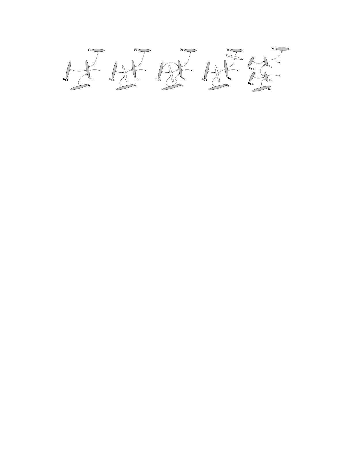
How to Construct Deep Recurrent Neural Networks Razvan P ascanu 1 , Caglar Gulcehre 1 , Kyungh yun Cho 2 , and Y oshua Bengio 1 1 D ´ epartement d’Informatique et de Recherche Op ´ erationelle, Univ ersit ´ e de Montr ´ eal, { pascanur, gulcehrc } @iro.umontreal.ca, yoshua.bengio@umontreal.ca 2 Department of Information and Computer Science, Aalto Univ ersity School of Science, kyunghyun.cho@aalto.fi Abstract In this paper , we explore different ways to extend a recurrent neural network (RNN) to a deep RNN. W e start by arguing that the concept of depth in an RNN is not as clear as it is in feedforward neural networks. By carefully analyzing and understanding the architecture of an RNN, howe ver , we find three points of an RNN which may be made deeper; (1) input-to-hidden function, (2) hidden-to- hidden transition and (3) hidden-to-output function. Based on this observ ation, we propose tw o nov el architectures of a deep RNN which are orthogonal to an earlier attempt of stacking multiple recurrent layers to b uild a deep RNN (Schmidhu- ber, 1992; El Hihi and Bengio, 1996). W e provide an alternative interpretation of these deep RNNs using a nov el frame work based on neural operators. The proposed deep RNNs are empirically ev aluated on the tasks of polyphonic music prediction and language modeling. The experimental result supports our claim that the proposed deep RNNs benefit from the depth and outperform the con ven- tional, shallow RNNs. 1 Introduction Recurrent neural networks (RNN, see, e.g., Rumelhart et al. , 1986) ha ve recently become a popular choice for modeling v ariable-length sequences. RNNs ha ve been successfully used for various task such as language modeling (see, e.g., Gra ves, 2013; Pascanu et al. , 2013a; Mikolov, 2012; Sutske ver et al. , 2011), learning word embeddings (see, e.g., Mikolov et al. , 2013a), online handwritten recog- nition (Grav es et al. , 2009) and speech recognition (Grav es et al. , 2013). In this work, we e xplore deep extensions of the basic RNN. Depth for feedforward models can lead to more expressi ve models (Pascanu et al. , 2013b), and we believ e the same should hold for recurrent models. W e claim that, unlike in the case of feedforward neural networks, the depth of an RNN is ambiguous. In one sense, if we consider the e xistence of a composition of sev eral nonlinear computational layers in a neural network being deep, RNNs are already deep, since any RNN can be expressed as a composition of multiple nonlinear layers when unfolded in time. Schmidhuber (1992); El Hihi and Bengio (1996) earlier proposed another way of building a deep RNN by stacking multiple recurrent hidden states on top of each other . This approach poten- tially allows the hidden state at each level to operate at different timescale (see, e.g., Hermans and Schrauwen, 2013). Nonetheless, we notice that there are some other aspects of the model that may still be considered shallow . For instance, the transition between two consecuti ve hidden states at a single lev el is shallow , when vie wed separately .This has implications on what kind of transitions this model can represent as discussed in Section 3.2.3. Based on this observation, in this paper, we inv estigate possible approaches to extending an RNN into a deep RNN. W e begin by studying which parts of an RNN may be considered shallow . Then, 1 for each shallo w part, we propose an alternative deeper design, which leads to a number of deeper variants of an RNN. The proposed deeper variants are then empirically e valuated on two sequence modeling tasks. The layout of the paper is as follows. In Section 2 we briefly introduce the concept of an RNN. In Section 3 we explore dif ferent concepts of depth in RNNs. In particular, in Section 3.3.1–3.3.2 we propose two novel variants of deep RNNs and ev aluate them empirically in Section 5 on two tasks: polyphonic music prediction (Boulanger-Le wando wski et al. , 2012) and language modeling. Finally we discuss the shortcomings and advantages of the proposed models in Section 6. 2 Recurrent Neural Networks A recurrent neural network (RNN) is a neural network that simulates a discrete-time dynamical system that has an input x t , an output y t and a hidden state h t . In our notation the subscript t represents time. The dynamical system is defined by h t = f h ( x t , h t − 1 ) (1) y t = f o ( h t ) , (2) where f h and f o are a state transition function and an output function, respecti vely . Each function is parameterized by a set of parameters; θ h and θ o . Giv en a set of N training sequences D = n ( x ( n ) 1 , y ( n ) 1 ) , . . . , ( x ( n ) T n , y ( n ) T n ) o N n =1 , the parameters of an RNN can be estimated by minimizing the following cost function: J ( θ ) = 1 N N X n =1 T n X t =1 d ( y ( n ) t , f o ( h ( n ) t )) , (3) where h ( n ) t = f h ( x ( n ) t , h ( n ) t − 1 ) and h ( n ) 0 = 0 . d ( a , b ) is a predefined diver gence measure between a and b , such as Euclidean distance or cross-entropy . 2.1 Con ventional Recurr ent Neural Networks A con ventional RNN is constructed by defining the transition function and the output function as h t = f h ( x t , h t − 1 ) = φ h  W > h t − 1 + U > x t  (4) y t = f o ( h t , x t ) = φ o  V > h t  , (5) where W , U and V are respectively the transition, input and output matrices, and φ h and φ o are element-wise nonlinear functions. It is usual to use a saturating nonlinear function such as a logistic sigmoid function or a hyperbolic tangent function for φ h . An illustration of this RNN is in Fig. 2 (a). The parameters of the con ventional RNN can be estimated by , for instance, stochastic gradient de- scent (SGD) algorithm with the gradient of the cost function in Eq. (3) computed by backpropagation through time (Rumelhart et al. , 1986). 3 Deep Recurrent Neural Networks 3.1 Why Deep Recurrent Neural Networks? Deep learning is built around a hypothesis that a deep, hierarchical model can be exponentially more ef ficient at representing some functions than a shallo w one (Bengio, 2009). A number of recent theoretical results support this hypothesis (see, e.g., Le Roux and Bengio, 2010; Delalleau and Bengio, 2011; Pascanu et al. , 2013b). For instance, it has been shown by Delalleau and Bengio (2011) that a deep sum-product network may require exponentially less units to represent the same function compared to a shallow sum-product network. Furthermore, there is a wealth of empirical evidences supporting this hypothesis (see, e.g., Goodfellow et al. , 2013; Hinton et al. , 2012b,a). These findings make us suspect that the same ar gument should apply to recurrent neural networks. 2 3.2 Depth of a Recurr ent Neural Network y t- 1 x t- 1 h t- 1 x t h t y t x t+1 h t+1 y t+1 Figure 1: A con ventional recurrent neural netw ork unfolded in time. The depth is defined in the case of feedforward neural netw orks as having multiple nonlinear layers between input and output. Unfortunately this definition does not apply tri vially to a recurrent neural network (RNN) because of its temporal structure. For instance, any RNN when unfolded in time as in Fig. 1 is deep, because a computational path between the input at time k < t to the output at time t crosses se veral nonlinear layers. A close analysis of the computation carried out by an RNN (see Fig. 2 (a)) at each time step indi vid- ually , howe ver , sho ws that certain transitions are not deep, but are only results of a linear projection followed by an element-wise nonlinearity . It is clear that the hidden-to-hidden ( h t − 1 → h t ), hidden- to-output ( h t → y t ) and input-to-hidden ( x t → h t ) functions are all shallow in the sense that there exists no intermediate, nonlinear hidden layer . W e can no w consider dif ferent types of depth of an RNN by considering those transitions separately . W e may make the hidden-to-hidden transition deeper by having one or more intermediate nonlinear layers between two consecuti ve hidden states ( h t − 1 and h t ). At the same time, the hidden-to- output function can be made deeper , as described previously , by plugging, multiple intermediate nonlinear layers between the hidden state h t and the output y t . Each of these choices has a dif ferent implication. 3.2.1 Deep Input-to-Hidden Function A model can exploit more non-temporal structure from the input by making the input-to-hidden function deep. Previous work has shown that higher-lev el representations of deep networks tend to better disentangle the underlying factors of v ariation than the original input (Goodfellow et al. , 2009; Glorot et al. , 2011b) and flatten the manifolds near which the data concentrate (Bengio et al. , 2013). W e hypothesize that such higher-le vel representations should make it easier to learn the temporal structure between successiv e time steps because the relationship between abstract features can gen- erally be expressed more easily . This has been, for instance, illustrated by the recent w ork (Mikolo v et al. , 2013b) sho wing that word embeddings from neural language models tend to be related to their temporal neighbors by simple algebraic relationships, with the same type of relationship (adding a vector) holding o ver very dif ferent regions of the space, allo wing a form of analogical reasoning. This approach of making the input-to-hidden function deeper is in the line with the standard practice of replacing input with e xtracted features in order to improv e the performance of a machine learning model (see, e.g., Bengio, 2009). Recently , Chen and Deng (2013) reported that a better speech recognition performance could be achieved by emplo ying this strate gy , although the y did not jointly train the deep input-to-hidden function together with other parameters of an RNN. 3.2.2 Deep Hidden-to-Output Function A deep hidden-to-output function can be useful to disentangle the factors of variations in the hidden state, making it easier to predict the output. This allows the hidden state of the model to be more compact and may result in the model being able to summarize the history of previous inputs more efficiently . Let us denote an RNN with this deep hidden-to-output function a deep output RNN (DO-RNN). Instead of having feedforward, intermediate layers between the hidden state and the output, Boulanger-Le wando wski et al. (2012) proposed to replace the output layer with a conditional gen- 3 x t h t- 1 h t y t x t h t- 1 h t y t x t h t- 1 h t y t x t h t- 1 h t y t x t h t- 1 h t y t z t- 1 z t (a) RNN (b) DT -RNN (b*) DT(S)-RNN (c) DO T -RNN (d) Stacked RNN Figure 2: Illustrations of four different recurrent neural networks (RNN). (a) A con ventional RNN. (b) Deep T ransition (DT) RNN. (b*) DT -RNN with shortcut connections (c) Deep Transition, Deep Output (DO T) RNN. (d) Stacked RNN erativ e model such as restricted Boltzmann machines or neural autoregressiv e distribution estima- tor (Larochelle and Murray, 2011). In this paper we only consider feedforward intermediate layers. 3.2.3 Deep Hidden-to-Hidden T ransition The third knob we can play with is the depth of the hidden-to-hidden transition. The state transition between the consecutive hidden states effecti vely adds a new input to the summary of the previous inputs represented by the fixed-length hidden state. Previous w ork with RNNs has generally limited the architecture to a shallow operation; af fine transformation followed by an element-wise nonlin- earity . Instead, we argue that this procedure of constructing a ne w summary , or a hidden state, from the combination of the previous one and the new input should be highly nonlinear . This nonlinear transition could allow , for instance, the hidden state of an RNN to rapidly adapt to quickly changing modes of the input, while still preserving a useful summary of the past. This may be impossible to be modeled by a function from the family of generalized linear models. Howe ver , this highly non- linear transition can be modeled by an MLP with one or more hidden layers which has an universal approximator property (see, e.g., Hornik et al. , 1989). An RNN with this deep transition will be called a deep transition RNN (DT -RNN) throughout re- mainder of this paper . This model is shown in Fig. 2 (b). This approach of having a deep transition, howe ver , introduces a potential problem. As the in- troduction of deep transition increases the number of nonlinear steps the gradient has to tra verse when propagated back in time, it might become more difficult to train the model to capture long- term dependencies (Bengio et al. , 1994). One possible way to address this difficulty is to introduce shortcut connections (see, e.g., Raiko et al. , 2012) in the deep transition, where the added shortcut connections provide shorter paths, skipping the intermediate layers, through which the gradient is propagated back in time. W e refer to an RNN having deep transition with shortcut connections by DT(S)-RNN (See Fig. 2 (b*)). Furthermore, we will call an RNN having both a deep hidden-to-output function and a deep transi- tion a deep output, deep transition RNN (DOT -RNN). See Fig. 2 (c) for the illustration of DO T -RNN. If we consider shortcut connections as well in the hidden to hidden transition, we call the resulting model DO T(S)-RNN. An approach similar to the deep hidden-to-hidden transition has been proposed recently by Pinheiro and Collobert (2014) in the context of parsing a static scene. They introduced a recurrent con volu- tional neural netw ork (RCNN) which can be understood as a recurrent netw ork whose the transition between consecutive hidden states (and input to hidden state) is modeled by a con volutional neural network. The RCNN was shown to speed up scene parsing and obtained the state-of-the-art result in Stanford Background and SIFT Flow datasets. Ko and Dieter (2009) proposed deep transitions for Gaussian Process models. Earlier , V alpola and Karhunen (2002) used a deep neural network to model the state transition in a nonlinear , dynamical state-space model. 3.2.4 Stack of Hidden States An RNN may be extended deeper in yet another way by stacking multiple recurrent hidden layers on top of each other (Schmidhuber, 1992; El Hihi and Bengio, 1996; Jaeger, 2007; Graves, 2013). 4 W e call this model a stacked RNN (sRNN) to distinguish it from the other proposed variants. The goal of a such model is to encourage each recurrent lev el to operate at a different timescale. It should be noticed that the DT -RNN and the sRNN extend the con ventional, shallow RNN in different aspects. If we look at each recurrent le vel of the sRNN separately , it is easy to see that the transition between the consecutiv e hidden states is still shallow . As we hav e argued above, this limits the family of functions it can represent. For e xample, if the structure of the data is sufficiently complex, incorporating a ne w input frame into the summary of what had been seen up to no w might be an arbitrarily complex function. In such a case we would like to model this function by something that has universal approximator properties, as an MLP . The model can not rely on the higher layers to do so, because the higher layers do not feed back into the lower layer . On the other hand, the sRNN can deal with multiple time scales in the input sequence, which is not an obvious feature of the DT -RNN. The DT -RNN and the sRNN are, howe ver , orthogonal in the sense that it is possible to hav e both features of the DT -RNN and the sRNN by stacking multiple levels of DT -RNNs to build a stacked DT -RNN which we do not explore more in this paper . 3.3 Formal descriptions of deep RNNs Here we giv e a more formal description on how the deep transition recurrent neural network (DT - RNN) and the deep output RNN (DO-RNN) as well as the stacked RNN are implemented. 3.3.1 Deep T ransition RNN W e noticed from the state transition equation of the dynamical system simulated by RNNs in Eq. (1) that there is no restriction on the form of f h . Hence, we propose here to use a multilayer perceptron to approximate f h instead. In this case, we can implement f h by L intermediate layers such that h t = f h ( x t , h t − 1 ) = φ h  W > L φ L − 1  W > L − 1 φ L − 2  · · · φ 1  W > 1 h t − 1 + U > x t  , where φ l and W l are the element-wise nonlinear function and the weight matrix for the l -th layer . This RNN with a multilayered transition function is a deep transition RNN (DT -RNN). An illustration of building an RNN with the deep state transition function is sho wn in Fig. 2 (b). In the illustration the state transition function is implemented with a neural network with a single intermediate layer . This formulation allows the RNN to learn a non-tri vial, highly nonlinear transition between the consecutiv e hidden states. 3.3.2 Deep Output RNN Similarly , we can use a multilayer perceptron with L intermediate layers to model the output function f o in Eq. (2) such that y t = f o ( h t ) = φ o  V > L φ L − 1  V > L − 1 φ L − 2  · · · φ 1  V > 1 h t  , where φ l and V l are the element-wise nonlinear function and the weight matrix for the l -th layer . An RNN implementing this kind of multilayered output function is a deep output recurrent neural network (DO-RNN). Fig. 2 (c) draws a deep output, deep transition RNN (DOT -RNN) implemented using both the deep transition and the deep output with a single intermediate layer each. 3.3.3 Stacked RNN The stacked RNN (Schmidhuber, 1992; El Hihi and Bengio, 1996) has multiple levels of transition functions defined by h ( l ) t = f ( l ) h ( h ( l − 1) t , h ( l ) t − 1 ) = φ h  W > l h ( l ) t − 1 + U > l h ( l − 1) t  , 5 where h ( l ) t is the hidden state of the l -th level at time t . When l = 1 , the state is computed using x t instead of h ( l − 1) t . The hidden states of all the lev els are recursi vely computed from the bottom le vel l = 1 . Once the top-le vel hidden state is computed, the output can be obtained using the usual formula- tion in Eq. (5). Alternatively , one may use all the hidden states to compute the output (Hermans and Schrauwen, 2013). Each hidden state at each lev el may also be made to depend on the input as well (Grav es, 2013). Both of them can be considered approaches using shortcut connections discussed earlier . The illustration of this stacked RNN is in Fig. 2 (d). 4 Another Perspectiv e: Neural Operators In this section, we briefly introduce a nov el approach with which the already discussed deep tran- sition (DT) and/or deep output (DO) recurrent neural networks (RNN) may be built. W e call this approach which is based on building an RNN with a set of predefined neural operators, an operator - based framew ork. In the operator-based framework, one first defines a set of operators of which each is implemented by a multilayer perceptron (MLP). For instance, a plus operator ⊕ may be defined as a function receiving tw o vectors x and h and returning the summary h 0 of them: h 0 = x ⊕ h , where we may constrain that the dimensionality of h and h 0 are identical. Additionally , we can define another operator B which pr edicts the most likely output symbol x 0 giv en a summary h , such that x 0 = B h It is possible to define man y other operators, but in this paper , we stick to these tw o operators which are sufficient to e xpress all the proposed types of RNNs. x t h t- 1 h t y t + Figure 3: A view of an RNN under the operator-based framework: ⊕ and B are the plus and pr edict operators, respec- tiv ely . It is clear to see that the plus operator ⊕ and the predict operator B correspond to the transition function and the output function in Eqs. (1)–(2). Thus, at each step, an RNN can be thought as performing the plus operator to update the hidden state gi ven an input ( h t = x t ⊕ h t − 1 ) and then the predict operator to compute the output ( y t = B h t = B ( x t ⊕ h t − 1 ) ). See Fig. 3 for the illustration of how an RNN can be understood from the operator-based framew ork. Each operator can be parameterized as an MLP with one or more hidden layers, hence a neural operator, since we cannot simply expect the operation will be linear with respect to the input vector(s). By using an MLP to im- plement the operators, the proposed deep transition, deep output RNN (DO T -RNN) naturally arises. This framework provides us an insight on how the con- structed RNN be regularized. For instance, one may regularize the model such that the plus operator ⊕ is commutati ve. Howe ver , in this paper , we do not explore further on this approach. Note that this is different from (Mikolo v et al. , 2013a) where the learned embeddings of words happened to be suitable for algebraic operators. The operator-based framework proposed here is rather geared tow ard learning these operators directly . 5 Experiments W e train four types of RNNs described in this paper on a number of benchmark datasets to ev aluate their performance. For each benchmark dataset, we try the task of predicting the ne xt symbol. 6 The task of predicting the next symbol is equivalent to the task of modeling the distribution over a sequence. For each sequence ( x 1 , . . . , x T ) , we decompose it into p ( x 1 , . . . , x T ) = p ( x 1 ) T Y t =2 p ( x t | x 1 , . . . , x t − 1 ) , and each term on the right-hand side will be replaced with a single timestep of an RNN. In this setting, the RNN predicts the probability of the next symbol x t in the sequence giv en the all previous symbols x 1 , . . . x t − 1 . Then, we train the RNN by maximizing the log-likelihood. W e try this task of modeling the joint distribution on three dif ferent tasks; polyphonic music predic- tion, character-le vel and w ord-lev el language modeling. W e test the RNNs on the task of polyphonic music prediction using three datasets which are Notting- ham, JSB Chorales and MuseData (Boulanger -Le wandowski et al. , 2012). On the task of character- lev el and word-le vel language modeling, we use Penn T reebank Corpus (Marcus et al. , 1993). 5.1 Model Descriptions W e compare the conv entional recurrent neural network (RNN), deep transition RNN with shortcut connections in the transition MLP (DT(S)-RNN), deep output/transition RNN with shortcut connec- tions in the hidden to hidden transition MLP (DOT(S)-RNN) and stacked RNN (sRNN). See Fig. 2 (a)–(d) for the illustrations of these models. RNN DT(S)-RNN DO T(S)-RNN sRNN 2 layers Music Notthingam # units # parameters 600 465K 400,400 585K 400,400,400 745K 400 550K JSB Chorales # units # parameters 200 75K 400,400 585K 400,400,400 745K 400 550K MuseData # units # parameters 600 465K 400,400 585K 400,400,400 745K 600 1185K Language Char-le vel # units # parameters 600 420K 400,400 540K 400,400,600 790K 400 520K W ord-le vel # units # parameters 200 4.04M 200,200 6.12M 200,200,200 6.16M 400 8.48M T able 1: The sizes of the trained models. W e provide the number of hidden units as well as the total number of parameters. For DT(S)-RNN, the two numbers provided for the number of units mean the size of the hidden state and that of the intermediate layer , respecti vely . For DOT(S)-RNN, the three numbers are the size of the hidden state, that of the intermediate layer between the consecuti ve hidden states and that of the intermediate layer between the hidden state and the output layer . For sRNN, the number corresponds to the size of the hidden state at each lev el The size of each model is chosen from a limited set { 100 , 200 , 400 , 600 , 800 } to minimize the val- idation error for each polyphonic music task (See T able. 1 for the final models). In the case of language modeling tasks, we chose the size of the models from { 200 , 400 } and { 400 , 600 } for word-le vel and character-le vel tasks, respecti vely . In all cases, we use a logistic sigmoid function as an element-wise nonlinearity of each hidden unit. Only for the character-le vel language modeling we used rectified linear units (Glorot et al. , 2011a) for the intermediate layers of the output function, which gav e lower v alidation error . 5.2 T raining W e use stochastic gradient descent (SGD) and emplo y the strategy of clipping the gradient proposed by Pascanu et al. (2013a). Training stops when the v alidation cost stops decreasing. Polyphonic Music Prediction : For Nottingham and MuseData datasets we compute each gradient step on subsequences of at most 200 steps, while we use subsequences of 50 steps for JSB Chorales. 7 W e do not reset the hidden state for each subsequence, unless the subsequence belongs to a dif ferent song than the previous subsequence. The cutof f threshold for the gradients is set to 1. The hyperparameter for the learning rate schedule 1 is tuned manually for each dataset. W e set the hyperparameter β to 2330 for Nottingham, 1475 for MuseData and 100 for JSB Chroales. They correspond to two epochs, a single epoch and a third of an epoch, respectiv ely . The weights of the connections between any pair of hidden layers are sparse, having only 20 non- zero incoming connections per unit (see, e.g., Sutsk ev er et al. , 2013). Each weight matrix is rescaled to have a unit lar gest singular v alue (P ascanu et al. , 2013a). The weights of the connections between the input layer and the hidden state as well as between the hidden state and the output layer are initialized randomly from the white Gaussian distribution with its standard de viation fixed to 0 . 1 and 0 . 01 , respectiv ely . In the case of deep output functions (DOT(S)-RNN), the weights of the connections between the hidden state and the intermediate layer are sampled initially from the white Gaussian distribution of standard de viation 0 . 01 . In all cases, the biases are initialized to 0 . T o regularize the models, we add white Gaussian noise of standard deviation 0 . 075 to each weight parameter ev ery time the gradient is computed (Grav es, 2011). Language Modeling : W e used the same strategy for initializing the parameters in the case of lan- guage modeling. For character-le vel modeling, the standard deviations of the white Gaussian distri- butions for the input-to-hidden weights and the hidden-to-output weights, we used 0 . 01 and 0 . 001 , respectiv ely , while those hyperparameters were both 0 . 1 for word-le vel modeling. In the case of DO T(S)-RNN, we sample the weights of between the hidden state and the rectifier intermediate layer of the output function from the white Gaussian distribution of standard deviation 0 . 01 . When using rectifier units (character-based language modeling) we fix the biases to 0 . 1 . In language modeling, the learning rate starts from an initial value and is halved each time the vali- dation cost does not decrease significantly (Mikolov et al. , 2010). W e do not use any regularization for the character -le vel modeling, b ut for the w ord-lev el modeling we use the same strate gy of adding weight noise as we do with the polyphonic music prediction. For all the tasks (polyphonic music prediction, character-le vel and word-lev el language modeling), the stacked RNN and the DO T(S)-RNN were initialized with the weights of the con ventional RNN and the DT(S)-RNN, which is similar to layer-wise pretraining of a feedforward neural network (see, e.g., Hinton and Salakhutdinov, 2006). W e use a ten times smaller learning rate for each parameter that was pretrained as either RNN or DT(S)-RNN. RNN DT(S)-RNN DO T(S)-RNN sRNN DO T(S)-RNN* Notthingam 3 . 225 3 . 206 3 . 215 3 . 258 2 . 95 JSB Chorales 8 . 338 8 . 278 8 . 437 8 . 367 7 . 92 MuseData 6 . 990 6 . 988 6 . 973 6 . 954 6 . 59 T able 2: The performances of the four types of RNNs on the polyphonic music prediction. The numbers represent negativ e log-probabilities on test sequences. (*) W e obtained these results using DO T(S)-RNN with L p units in the deep transition, maxout units in the deep output function and dropout (Gulcehre et al. , 2013). 5.3 Result and Analysis 5.3.1 Polyphonic Music Prediction The log-probabilities on the test set of each data are presented in the first four columns of T ab . 2. W e were able to observe that in all cases one of the proposed deep RNNs outperformed the con ventional, shallow RNN. Though, the suitability of each deep RNN depended on the data it was trained on. The best results obtained by the DT(S)-RNNs on Notthingam and JSB Chorales are close to, but 1 W e use at each update τ , the follo wing learning rate η τ = 1 1+ max(0 ,τ − τ 0 ) β , where τ 0 and β indicate respec- tiv ely when the learning rate starts decreasing and how quickly the learning rate decreases. In the experiment, we set τ 0 to coincide with the time when the validation error starts increasing for the first time. 8 worse than the result obtained by RNNs trained with the technique of fast dropout (FD) which are 3 . 09 and 8 . 01 , respecti vely (Bayer et al. , 2013). In order to quickly in vestigate whether the proposed deeper v ariants of RNNs may also benefit from the recent advances in feedforward neural networks, such as the use of non-saturating acti vation functions 2 and the method of dropout. W e hav e built another set of DO T(S)-RNNs that hav e the recently proposed L p units (Gulcehre et al. , 2013) in deep transition and maxout units (Goodfellow et al. , 2013) in deep output function. Furthermore, we used the method of dropout (Hinton et al. , 2012b) instead of weight noise during training. Similarly to the pre viously trained models, we searched for the size of the models as well as other learning hyperparameters that minimize the validation performance. W e, howe ver , did not pretrain these models. The results obtained by the DO T(S)-RNNs having L p and maxout units trained with dropout are shown in the last column of T ab. 2. On every music dataset the performance by this model is sig- nificantly better than those achie ved by all the other models as well as the best results reported with recurrent neural netw orks in (Bayer et al. , 2013). This suggests us that the proposed v ariants of deep RNNs also benefit from having non-saturating activ ations and using dropout, just like feedforward neural networks. W e reported these results and more details on the experiment in (Gulcehre et al. , 2013). W e, howe ver , acknowledge that the model-free state-of-the-art results for the both datasets were obtained using an RNN combined with a conditional generativ e model, such as restricted Boltz- mann machines or neural autoregressiv e distrib ution estimator (Larochelle and Murray, 2011), in the output (Boulanger-Le wando wski et al. , 2012). RNN DT(S)-RNN DO T(S)-RNN sRNN ∗ ? Character-Le vel 1 . 414 1 . 409 1 . 386 1 . 412 1 . 41 1 1 . 24 3 W ord-Le vel 117 . 7 112 . 0 107 . 5 110 . 0 123 2 117 3 T able 3: The performances of the four types of RNNs on the tasks of language modeling. The numbers represent bit-per-character and perplexity computed on test sequence, respectiv ely , for the character-le vel and word-lev el modeling tasks. ∗ The previous/current state-of-the-art results obtained with shallo w RNNs. ? The previous/current state-of-the-art results obtained with RNNs having long-short term memory units. 5.3.2 Language Modeling On T ab . 3, we can see the perple xities on the test set achiev ed by the all four models. W e can clearly see that the deep RNNs (DT(S)-RNN, DO T(S)-RNN and sRNN) outperform the con ventional, shal- low RNN significantly . On these tasks DO T(S)-RNN outperformed all the other models, which suggests that it is important to ha ve highly nonlinear mapping from the hidden state to the output in the case of language modeling. The results by both the DOT(S)-RNN and the sRNN for word-le vel modeling surpassed the previous best performance achieved by an RNN with 1000 long short-term memory (LSTM) units (Grav es, 2013) as well as that by a shallow RNN with a larger hidden state (Mik olov et al. , 2011), ev en when both of them used dynamic ev aluation 3 . The results we report here are without dynamic e valuation. For character -lev el modeling the state-of-the-art results were obtained using an optimization method Hessian-free with a specific type of RNN architecture called mRNN (Mikolo v et al. , 2012a) or a regularization technique called adaptive weight noise (Graves, 2013). Our result, howe ver , is better than the performance achie ved by con ventional, shallow RNNs without any of those adv anced 2 Note that it is not tri vial to use non-saturating activ ation functions in conv entional RNNs, as this may cause the explosion of the activ ations of hidden states. Ho wev er, it is perfectly safe to use non-saturating activ ation functions at the intermediate layers of a deep RNN with deep transition. 1 Reported by Mikolov et al. (2012a) using mRNN with Hessian-free optimization technique. 2 Reported by Mikolov et al. (2011) using the dynamic e v aluation. 3 Reported by Grav es (2013) using the dynamic ev aluation and weight noise. 3 Dynamic ev aluation refers to an approach where the parameters of a model are updated as the valida- tion/test data is predicted. 9 regularization methods (Mikolov et al. , 2012b), where they reported the best performance of 1 . 41 using an RNN trained with the Hessian-free learning algorithm (Martens and Sutske ver, 2011). 6 Discussion In this paper , we have explored a no vel approach to building a deep recurrent neural network (RNN). W e considered the structure of an RNN at each timestep, which rev ealed that the relationship be- tween the consecuti ve hidden states and that between the hidden state and output are shallow . Based on this observation, we proposed two alternativ e designs of deep RNN that make those shallow re- lationships be modeled by deep neural netw orks. Furthermore, we proposed to make use of shortcut connections in these deep RNNs to alleviate a problem of difficult learning potentially introduced by the increasing depth. W e empirically ev aluated the proposed designs against the con ventional RNN which has only a single hidden layer and against another approach of building a deep RNN (stacked RNN, Grav es, 2013), on the task of polyphonic music prediction and language modeling. The experiments re vealed that the RNN with the proposed deep transition and deep output (DO T(S)- RNN) outperformed both the conv entional RNN and the stacked RNN on the task of language modeling, achie ving the state-of-the-art result on the task of word-lev el language modeling. F or polyphonic music prediction, a different deeper variant of an RNN achieved the best performance for each dataset. Importantly , howe ver , in all the cases, the con ventional, shallo w RNN was not able to outperform the deeper v ariants. These results strongly support our claim that an RNN benefits from having a deeper architecture, just lik e feedforward neural networks. The observation that there is no clear winner in the task of polyphonic music prediction suggests us that each of the proposed deep RNNs has a distinct characteristic that makes it more, or less, suitable for certain types of datasets. W e suspect that in the future it will be possible to design and train yet another deeper variant of an RNN that combines the proposed models together to be more robust to the characteristics of datasets. For instance, a stacked DT(S)-RNN may be constructed by combining the DT(S)-RNN and the sRNN. In a quick additional experiment where we hav e trained DO T(S)-RNN constructed using non- saturating nonlinear activ ation functions and trained with the method of dropout, we were able to improv e the performance of the deep recurrent neural networks on the polyphonic music prediction tasks significantly . This suggests us that it is important to in v estigate the possibility of applying recent adv ances in feedforward neural networks, such as novel, non-saturating activ ation functions and the method of dropout, to recurrent neural networks as well. Howe ver , we leave this as future research. One practical issue we ran into during the e xperiments w as the dif ficulty of training deep RNNs. W e were able to train the con ventional RNN as well as the DT(S)-RNN easily , but it was not tri vial to train the DO T(S)-RNN and the stacked RNN. In this paper , we proposed to use shortcut connections as well as to pretrain them either with the con ventional RNN or with the DT(S)-RNN. W e, howe ver , believ e that learning may become ev en more problematic as the size and the depth of a model increase. In the future, it will be important to in vestigate the root causes of this difficulty and to explore potential solutions. W e find some of the recently introduced approaches, such as advanced regularization methods (Pascanu et al. , 2013a) and advanced optimization algorithms (see, e.g., Pascanu and Bengio, 2013; Martens, 2010), to be promising candidates. Acknowledgments W e would like to thank the developers of Theano (Bergstra et al. , 2010; Bastien et al. , 2012). W e also thank Justin Bayer for his insightful comments on the paper . W e would like to thank NSERC, Compute Canada, and Calcul Qu ´ ebec for providing computational resources. Razvan Pascanu is supported by a DeepMind Fellowship. Kyunghyun Cho is supported by FICS (Finnish Doctoral Programme in Computational Sciences) and “the Academy of Finland (Finnish Centre of Excellence in Computational Inference Research COIN, 251170)”. 10 References Bastien, F ., Lamblin, P ., Pascanu, R., Ber gstra, J., Goodfellow , I. J., Ber geron, A., Bouchard, N., and Bengio, Y . (2012). Theano: new features and speed improvements. Deep Learning and Unsupervised Feature Learning NIPS 2012 W orkshop. Bayer , J., Osendorfer , C., Korhammer , D., Chen, N., Urban, S., and van der Smagt, P . (2013). On fast dropout and its applicability to recurrent networks. arXiv: 1311.0701 [cs.NE] . Bengio, Y . (2009). Learning deep architectures for AI. F ound. T r ends Mach. Learn. , 2 (1), 1–127. Bengio, Y ., Simard, P ., and Frasconi, P . (1994). Learning long-term dependencies with gradient descent is difficult. IEEE T ransactions on Neural Networks , 5 (2), 157–166. Bengio, Y ., Mesnil, G., Dauphin, Y ., and Rifai, S. (2013). Better mixing via deep representations. In ICML ’13 . Bergstra, J., Breuleux, O., Bastien, F ., Lamblin, P ., Pascanu, R., Desjardins, G., T urian, J., W arde- Farle y , D., and Bengio, Y . (2010). Theano: a CPU and GPU math e xpression compiler . In Pr oceedings of the Python for Scientific Computing Confer ence (SciPy) . Oral Presentation. Boulanger-Le wando wski, N., Bengio, Y ., and V incent, P . (2012). Modeling temporal dependencies in high-dimensional sequences: Application to polyphonic music generation and transcription. In ICML ’2012 . Chen, J. and Deng, L. (2013). A new method for learning deep recurrent neural networks. arXiv: 1311.6091 [cs.LG] . Delalleau, O. and Bengio, Y . (2011). Shallow vs. deep sum-product networks. In NIPS . El Hihi, S. and Bengio, Y . (1996). Hierarchical recurrent neural networks for long-term dependen- cies. In NIPS 8 . MIT Press. Glorot, X., Bordes, A., and Bengio, Y . (2011a). Deep sparse rectifier neural networks. In AIST ATS . Glorot, X., Bordes, A., and Bengio, Y . (2011b). Domain adaptation for large-scale sentiment classi- fication: A deep learning approach. In ICML ’2011 . Goodfellow , I., Le, Q., Saxe, A., and Ng, A. (2009). Measuring in v ariances in deep networks. In NIPS’09 , pages 646–654. Goodfellow , I. J., W arde-Farley , D., Mirza, M., Courville, A., and Bengio, Y . (2013). Maxout networks. In ICML ’2013 . Grav es, A. (2011). Practical variational inference for neural networks. In J. Shawe-T aylor , R. Zemel, P . Bartlett, F . Pereira, and K. W einberger , editors, Advances in Neural Information Pr ocessing Systems 24 , pages 2348–2356. Grav es, A. (2013). Generating sequences with recurrent neural networks. arXiv: 1308.0850 [cs.NE] . Grav es, A., Liwicki, M., Fernandez, S., Bertolami, R., Bunke, H., and Schmidhuber , J. (2009). A nov el connectionist system for improv ed unconstrained handwriting recognition. IEEE T ransac- tions on P attern Analysis and Machine Intellig ence . Grav es, A., Mohamed, A., and Hinton, G. (2013). Speech recognition with deep recurrent neural networks. ICASSP . Gulcehre, C., Cho, K., Pascanu, R., and Bengio, Y . (2013). Learned-norm pooling for deep feedfor- ward and recurrent neural networks. arXiv: 1311.1780 [cs.NE] . Hermans, M. and Schrauwen, B. (2013). T raining and analysing deep recurrent neural networks. In Advances in Neural Information Pr ocessing Systems 26 , pages 190–198. Hinton, G., Deng, L., Dahl, G. E., Mohamed, A., Jaitly , N., Senior , A., V anhoucke, V ., Nguyen, P ., Sainath, T ., and Kingsbury , B. (2012a). Deep neural networks for acoustic modeling in speech recognition. IEEE Signal Pr ocessing Magazine , 29 (6), 82–97. Hinton, G. E. and Salakhutdinov , R. (2006). Reducing the dimensionality of data with neural net- works. Science , 313 (5786), 504–507. Hinton, G. E., Sri vasta va, N., Krizhevsky , A., Sutskev er , I., and Salakhutdinov , R. (2012b). Im- proving neural networks by prev enting co-adaptation of feature detectors. T echnical report, 11 Hornik, K., Stinchcombe, M., and White, H. (1989). Multilayer feedforward networks are uni versal approximators. Neural Networks , 2 , 359–366. Jaeger , H. (2007). Discovering multiscale dynamical features with hierarchical echo state networks. T echnical report, Jacobs Univ ersity . K o, J. and Dieter, F . (2009). Gp-bayesfilters: Bayesian filtering using gaussian process prediction and observation models. Autonomous Robots . Larochelle, H. and Murray , I. (2011). The Neural Autoregressiv e Distribution Estimator . In Pr o- ceedings of the F ourteenth International Confer ence on Artificial Intelligence and Statistics (AIS- T A TS’2011) , v olume 15 of JMLR: W&CP . Le Roux, N. and Bengio, Y . (2010). Deep belief networks are compact univ ersal approximators. Neural Computation , 22 (8), 2192–2207. Marcus, M. P ., Marcinkiewicz, M. A., and Santorini, B. (1993). Building a large annotated corpus of english: The Penn Treebank. Computational Linguistics , 19 (2), 313–330. Martens, J. (2010). Deep learning via Hessian-free optimization. In L. Bottou and M. Littman, ed- itors, Pr oceedings of the T wenty-se venth International Conference on Machine Learning (ICML- 10) , pages 735–742. A CM. Martens, J. and Sutske ver , I. (2011). Learning recurrent neural networks with Hessian-free opti- mization. In Pr oc. ICML ’2011 . A CM. Mikolov , T . (2012). Statistical Language Models based on Neural Networks . Ph.D. thesis, Brno Univ ersity of T echnology . Mikolov , T ., Karafi ´ at, M., Burget, L., Cernocky , J., and Khudanpur , S. (2010). Recurrent neural network based language model. In Pr oceedings of the 11th Annual Confer ence of the International Speech Communication Association (INTERSPEECH 2010) , volume 2010, pages 1045–1048. International Speech Communication Association. Mikolov , T ., K ombrink, S., Bur get, L., Cernocky , J., and Khudanpur , S. (2011). Extensions of recur - rent neural network language model. In Proc. 2011 IEEE international conference on acoustics, speech and signal pr ocessing (ICASSP 2011) . Mikolov , T ., Sutske ver , I., Deoras, A., Le, H., K ombrink, S., and Cernocky , J. (2012a). Subword language modeling with neural networks. unpublished . Mikolov , T ., Sutske ver , I., Deoras, A., Le, H.-S., Kombrink, S., and Cernocky , J. (2012b). Subword language modeling with neural networks. preprint (http://www .fit.vutbr .cz/ imikolo v/rnnlm/char .pdf). Mikolov , T ., Sutskev er , I., Chen, K., Corrado, G., and Dean, J. (2013a). Distributed representations of words and phrases and their compositionality . In Advances in Neural Information Processing Systems 26 , pages 3111–3119. Mikolov , T ., Chen, K., Corrado, G., and Dean, J. (2013b). Efficient estimation of word represen- tations in vector space. In International Confer ence on Learning Representations: W orkshops T rack . Pascanu, R. and Bengio, Y . (2013). Revisiting natural gradient for deep netw orks. T echnical report, Pascanu, R., Mikolov , T ., and Bengio, Y . (2013a). On the dif ficulty of training recurrent neural networks. In ICML ’2013 . Pascanu, R., Montufar , G., and Bengio, Y . (2013b). On the number of response regions of deep feed forward networks with piece-wise linear acti v ations. arXiv: 1312.6098[cs.LG] . Pinheiro, P . and Collobert, R. (2014). Recurrent con volutional neural networks for scene labeling. In Pr oceedings of The 31st International Confer ence on Machine Learning , pages 82–90. Raiko, T ., V alpola, H., and LeCun, Y . (2012). Deep learning made easier by linear transformations in perceptrons. In Pr oceedings of the F ifteenth Internation Confer ence on Artificial Intelligence and Statistics (AIST A TS 2012) , volume 22 of JMLR W orkshop and Confer ence Pr oceedings , pages 924–932. JMLR W&CP . Rumelhart, D. E., Hinton, G. E., and W illiams, R. J. (1986). Learning representations by back- propagating errors. Natur e , 323 , 533–536. 12 Schmidhuber , J. (1992). Learning complex, extended sequences using the principle of history com- pression. Neural Computation , (4), 234–242. Sutske ver , I., Martens, J., and Hinton, G. (2011). Generating text with recurrent neural networks. In L. Getoor and T . Scheffer , editors, Pr oceedings of the 28th International Conference on Mac hine Learning (ICML 2011) , pages 1017–1024, Ne w Y ork, NY , USA. A CM. Sutske ver , I., Martens, J., Dahl, G., and Hinton, G. (2013). On the importance of initialization and momentum in deep learning. In ICML . V alpola, H. and Karhunen, J. (2002). An unsupervised ensemble learning method for nonlinear dynamic state-space models. Neural Comput. , 14 (11), 2647–2692. 13