GP-Localize: Persistent Mobile Robot Localization using Online Sparse Gaussian Process Observation Model

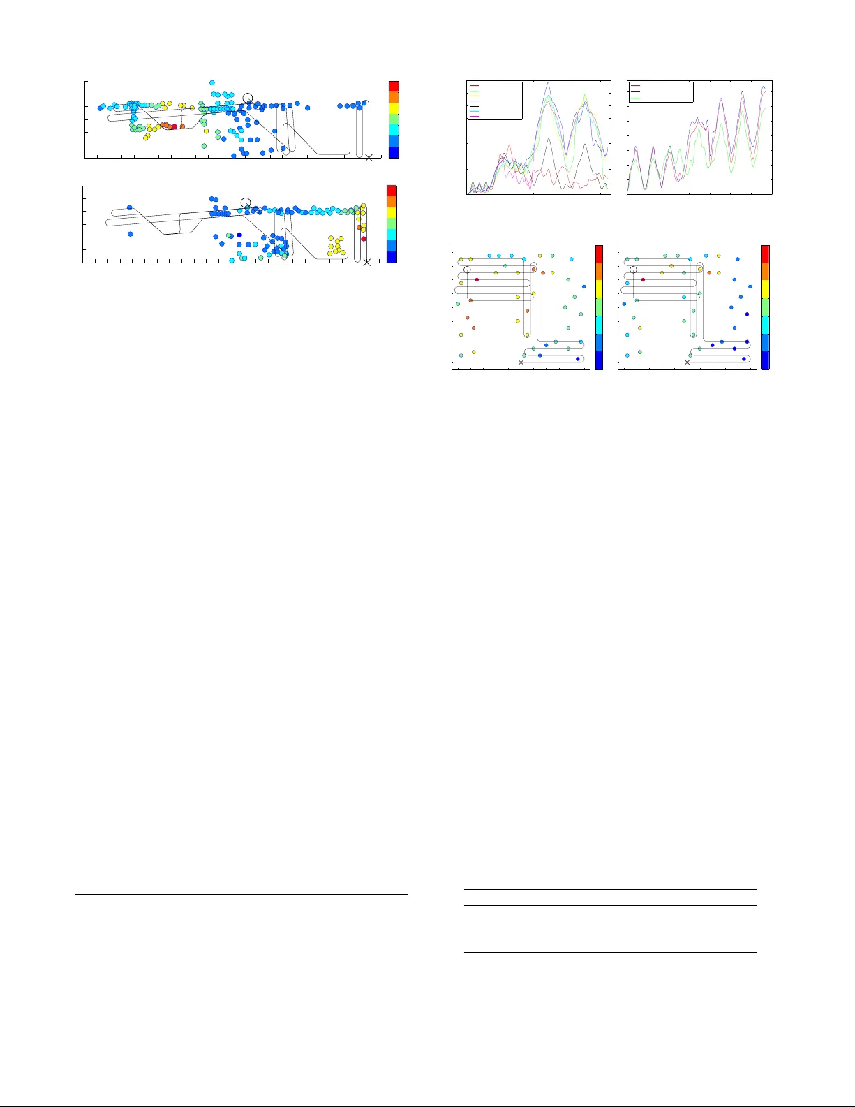
GP-Localize: P ersistent Mobile Robot Localization using Online Sparse Gaussian Pr ocess Observ ation Model Nuo Xu † and Kian Hsiang Low † and Jie Chen § and K eng Kiat Lim † and Etkin Baris ¸ ¨ Ozg ¨ ul † Department of Computer Science, National Univ ersity of Singapore, Republic of Singapore † Singapore-MIT Alliance for Research and T echnology , Republic of Singapore § { xunuo, lowkh, k engkiat, ebozgul } @comp.nus.edu.sg † , chenjie@smart.mit.edu § Abstract Central to robot exploration and mapping is the task of persistent localization in en vironmental fields character- ized by spatially correlated measurements. This paper presents a Gaussian pr ocess localization (GP-Localize) algorithm that, in contrast to e xisting w orks, can exploit the spatially correlated field measurements taken during a robot’ s exploration (instead of relying on prior train- ing data) for efficiently and scalably learning the GP observation model online through our proposed novel online sparse GP . As a result, GP-Localize is capable of achieving constant time and memory (i.e., independent of the size of the data) per filtering step, which demon- strates the practical feasibility of using GPs for persis- tent robot localization and autonomy . Empirical e v alua- tion via simulated experiments with real-world datasets and a real robot experiment shows that GP-Localize out- performs existing GP localization algorithms. 1 Introduction Recent research in robot exploration and mapping has fo- cused on developing adaptiv e sampling and active sensing algorithms (Cao, Low , and Dolan 2013; Chen, Lo w , and T an 2013; Chen et al. 2012; Hoang et al. 2014; Low , Dolan, and Khosla 2008; 2009; 2011; Lo w et al. 2007; 2012; Ouyang et al. 2014) to g ather the most informati ve data/observations for modeling and predicting spatially v arying environmen- tal fields that are characterized by continuous-valued , spa- tially corr elated measurements. Application domains (e.g., en vironmental sensing and monitoring) requiring such al- gorithms often contain multiple fields of interest: (a) Au- tonomous underwater and surface v ehicles are tasked to sample ocean and freshwater phenomena including temper- ature, salinity , and oxygen concentration fields (Dolan et al. 2009; Podnar et al. 2010), (b) indoor en vironments are spanned by temperature, light, and carbon dioxide concen- tration fields that af fect the occupants’ comfort and satis- faction to wards the en vironmental quality across dif ferent areas, and (c) WiFi access points/hotspots situated at neigh- boring locations produce dif ferent but overlapping wireless signal strength fields ov er the same en vironment. These al- gorithms operate with an assumption that the locations of ev- ery robot and its gathered observations are kno wn and pro- vided by its onboard sensors such as the widely-used GPS Copyright c  2014, Association for the Advancement of Artificial Intelligence (www .aaai.org). All rights reserved. device. Howe ver , GPS signals may be noisy (e.g., due to urban canyon effect between tall b uildings) or unav ailable (e.g., in underwater or indoor en vironments). So, it is desir- able to alternativ ely consider exploiting the spatially corre- lated measurements taken by each robot for localizing itself within the environmental fields during its exploration; this will significantly extend the range of en vironments and ap- plication domains in which a robot can localize itself. T o achiev e this, our robotics community will usually make use of a probabilistic state estimation frame work known as the Bayes filter : It repeatedly updates the belief of a robot’ s location/state by assimilating the field measure- ments taken during the robot’ s exploration through its ob- servation model . T o preserv e time efficienc y , the Bayes fil- ter imposes a Markov property on the observation model: Giv en the robot’ s current location, its current measurement is conditionally independent of the past measurements. Such a Markov property is severely violated by the spatial corre- lation structure of the environmental fields, thus strongly de- grading the robot’ s localization performance. T o resolve this issue, the works of Ko and Fox (2009a; 2009b) have inte- grated a rich class of Bayesian nonparametric models called the Gaussian pr ocess (GP) into the Bayes filter, which al- lows the spatial correlation structure between measurements to be formally characterized (i.e., by modeling each field as a GP) and the observation model to be represented by fully probabilistic predicti v e distributions (i.e., one per field/GP) with formal measures of the uncertainty of the predictions. Unfortunately , such expressi v e po wer of a GP comes at a high computational cost, which hinders its practical use in the Bayes filter for persistent robot localization: It incurs cubic time and quadratic memory in the size of the data/observations. Existing works (Brooks, Makarenko, and Upcroft 2008; Ferris, H ¨ ahnel, and F ox 2006; Fer - ris, Fox, and Lawrence 2007; K o and Fox 2009a; 2009b) hav e sidestepped this computational difficulty by assum- ing the av ailability of data/observations prior to exploration and localization for training the GP observ ation model of- fline; some (Brooks, Makarenk o, and Upcroft 2008; Ferris, H ¨ ahnel, and Fox 2006; Ko and Fox 2009a) hav e assumed these giv en prior measurements to be labeled with known locations while others (Ferris, Fox, and Lawrence 2007; K o and Fox 2009b) hav e inferred their location labels. The Markov assumption on the observ ation model can then be “relaxed” to conditional independence between the robot’ s current measurement and past measurements (i.e., taken during its exploration) given its current location and the trained GPs using prior data/observations, thus improving the efficienc y at each filtering step during its exploration to quadratic time in the size of the prior training data. Any mea- surement taken during the robot’ s actual exploration and lo- calization is thus not used to train the GP observ ation model. Such a “relaxed” Marko v assumption may hold in certain static environments. Howe v er , it becomes highly restricti ve and is easily violated in general, practical environmental set- tings where, for e xample, (a) limited sampling budget (i.e., in terms of energy consumption, mission time, etc.) for- bids the collection of prior training data or only permits ex- tremely sparse prior data to be gathered relative to a large en vironment, thus resulting in an inaccurately trained GP observation model, (b) en vironmental changes in v alidate the prior training data, and (c) the robot’ s actual exploration path is spatially distant from the prior observations, hence mak- ing the trained GP observation model uninformati ve to its lo- calization. All these practical considerations motiv ate us to tackle a fundamental research question: W ithout prior train- ing data, how can GPs be restructured to be used by a Bayes filter for per sistent robot localization in en vironmental fields characterized by spatially correlated measurements? This paper presents a Gaussian pr ocess localization (GP- Localize) algorithm that, in contrast to existing works men- tioned above, can e xploit the spatially correlated field mea- surements taken during a robot’ s exploration (instead of relying on prior training data) for ef ficiently and scalably learning the GP observ ation model online through our pro- posed no vel online sparse GP (Section 3). As a result, GP- Localize is capable of achieving constant time and memory (i.e., independent of the size of the data/observations) per filtering step, which we believe is an important first step to- wards demonstrating the practical feasibility of employing GPs for persistent robot localization and autonomy . W e em- pirically demonstrate through simulated experiments with three real-world datasets as well as a real robot e xperiment that GP-Localize outperforms existing GP localization algo- rithms (Section 4). 2 Background 2.1 Modeling En vir onmental Field with GP The Gaussian process (GP) can be used to model an envi- ronmental field as follows 1 : The en vironmental field is de- fined to vary as a realization of a GP . Let X be a set of lo- cations representing the domain of the en vironmental field such that each location x ∈ X is associated with a real- ized (random) field measurement z x ( Z x ) if x is observed (unobserved). Let { Z x } x ∈X denote a GP , that is, every fi- nite subset of { Z x } x ∈X has a multiv ariate Gaussian dis- tribution (Rasmussen and W illiams 2006). The GP is fully specified by its prior mean µ x , E [ Z x ] and cov ariance σ xx 0 , cov[ Z x , Z x 0 ] for all x, x 0 ∈ X , the latter of which characterizes the spatial correlation structure of the field 1 T o simplify exposition, we only describe the GP for a single field; for multiple fields, we assume independence between them to ease computations. and can be defined using a covariance function. A com- mon choice is the squared exponential co v ariance function σ xx 0 , σ 2 s exp {− 0 . 5( x − x 0 ) > M − 2 ( x − x 0 )+ σ 2 n δ xx 0 } where σ 2 s and σ 2 n are, respectiv ely , the signal and noise variance controlling the intensity and the noise of the measurements, M is a diagonal matrix with length-scale components ` 1 and ` 2 controlling, respectiv ely , the degree of spatial correlation or “similarity” between measurements in the horizontal and vertical directions of the field, and δ xx 0 is a Kronecker delta of value 1 if x = x 0 , and 0 otherwise. A chief advantage of using the full GP to model the en vi- ronmental field is its capability of performing probabilistic regression: Supposing a robot has visited and observ ed a set D of locations and taken a column v ector z D of correspond- ing realized measurements, the full GP can exploit these ob- servations to predict the measurement at any unobserv ed lo- cation x ∈ X \ D as well as pro vide its corresponding pre- dictiv e uncertainty using a Gaussian predictiv e distrib ution p ( z x | x, D , z D ) = N ( µ x |D , σ xx |D ) with the following pos- terior mean and variance, respecti vely: µ x |D , µ x + Σ x D Σ − 1 DD ( z D − µ D ) (1) σ xx |D , σ xx − Σ x D Σ − 1 DD Σ D x (2) where µ D is a column v ector with mean components µ x 0 for all x 0 ∈ D , Σ x D is a row vector with cov ariance components σ xx 0 for all x 0 ∈ D , Σ D x is the transpose of Σ x D , and Σ DD is a matrix with components σ x 0 x 00 for all x 0 , x 00 ∈ D . 2.2 Sparse Gaussian Process A ppr oximation The key limitation hindering the practical use of the full GP in the Bayes filter for persistent robot localization is its poor scalability in the size |D | of the data/observations: Comput- ing the Gaussian predicti v e distrib ution (i.e., (1) and (2)) re- quires inv erting the covariance matrix Σ DD , which incurs O ( |D | 3 ) time and O ( |D | 2 ) memory . T o improve its scala- bility , GP approximation methods (Chen et al. 2012; 2013; Qui ˜ nonero-Candela and Rasmussen 2005) hav e been pro- posed, two of which will be described belo w . The simple sparse subset of data (SoD) approximation method uses only a subset S of the set D of locations (i.e., S ⊂ D ) observed and the realized measurements z S taken by the robot to produce a Gaussian predictiv e distrib ution of the measurement at any unobserved location x ∈ X \ D with the following posterior mean and v ariance, which are simi- lar to that of full GP (i.e., by replacing D in (1) and (2) with S ): µ x |S = µ x + Σ x S Σ − 1 S S ( z S − µ S ) (3) σ xx |S = σ xx − Σ x S Σ − 1 S S Σ S x . (4) The cov ariance matrix Σ S S is in v erted using O ( |S | 3 ) time and O ( |S | 2 ) memory , which are independent of |D | . The main criticism of SoD is that it does not exploit all the data for computing the Gaussian predicti ve distribution, thus yielding an unrealistic o verestimate (4) of the predictiv e un- certainty (ev en with fairly redundant data and informati ve subset S ) (Qui ˜ nonero-Candela and Rasmussen 2005) and in turn an inaccurately trained observation model. The sparse partially independent training conditional (PITC) approximation method is the most general form of a class of reduced-rank cov ariance matrix approximation methods reported in (Qui ˜ nonero-Candela and Rasmussen 2005) exploiting the notion of a support set S ⊂ X . Un- like SoD, PITC can utilize all data (i.e., D and z D ) to deri ve a Gaussian predictiv e distribution of the measurement at any x ∈ X \ D with the following posterior mean and v ariance: µ PITC x |D , µ x + Γ x D (Γ DD + Λ) − 1 ( z D − µ D ) (5) σ PITC xx |D , σ xx − Γ x D (Γ DD + Λ) − 1 Γ D x (6) where Γ AA 0 = Σ AS Σ − 1 S S Σ S A 0 for all A , A 0 ⊂ X and Λ is a block-diagonal matrix constructed from the N diagonal blocks of Σ DD |S , each of which is a matrix Σ D n D n |S for n = 1 , · · · , N where D = S N n =1 D n . Also, unlike SoD, the support set S does not ha ve to be observed. The covariance matrix Σ DD in (1) and (2) is approximated by a reduced- rank matrix Γ DD summed with the resulting sparsified resid- ual matrix Λ in (5) and (6). So, computing either µ PITC x |D (5) or σ PITC xx |D (6), which requires inv erting the approximated covari- ance matrix Γ DD + Λ , incurs O ( |D | ( |S | 2 + ( |D | / N ) 2 )) time and O ( |S | 2 + ( |D| / N ) 2 ) memory . The sparse fully indepen- dent training conditional (FITC) approximation method is a special case of PITC where Λ is a diagonal matrix con- structed from σ x 0 x 0 |S for all x 0 ∈ D (i.e., N = |D | ). FITC is previously employed by Ko and Fox (2009a) to speed up the learning of observation model with prior training data. But, the time incurred by PITC or FITC gro ws with increas- ing size of data. So, it is computationally impractical to use them directly to repeatedly train the observation model at each filtering step for persistent localization. 2.3 Bayes Filters A Bayes filter is a probabilistic state estimation frame work that repeatedly updates the belief of a robot’ s location/state by conditioning on its control actions performed and field measurements taken so far . Formally , let the robot’ s con- trol action performed, its location visited and observed, and the corresponding realized field measurement taken at time/filtering step t be denoted by u t , x t , and z t 2 , respec- tiv ely . T o estimate the robot’ s location, a belief b ( x t ) , p ( x t | u 1: t , z 1: t ) is maintained ov er all its possible locations x t where u 1: t , ( u 1 , . . . , u t ) > and z 1: t , ( z 1 , . . . , z t ) > denote, respectively , column v ectors of past control actions performed and realized field measurements taken by the robot up until time step t . T o track such a belief, after the robot has performed an action u t and taken a realized mea- surement z t at each time step t , the Bayes filter updates the prior belief b ( x t − 1 ) of the robot’ s location to the poste- rior belief b ( x t ) = β p ( z t | x t ) R p ( x t | u t , x t − 1 ) b ( x t − 1 ) d x t − 1 where 1 /β is a normalizing constant, p ( x t | u t , x t − 1 ) is a mo- tion model representing the probability of the robot moving from locations x t − 1 to x t after performing action u t , and p ( z t | x t ) is an observation model describing the likelihood of taking realized measurement z t at location x t . T o preserve ef ficiency , the Bayes filter imposes a Markov property on the observation model: Giv en the robot’ s cur - rent location x t , its current measurement z t is conditionally 2 The field measurement z t is index ed by time step t instead of the corresponding location x t since x t is not known to the robot. independent of past actions u 1: t and measurements z 1: t − 1 : p ( z t | x t , u 1: t , z 1: t − 1 ) = p ( z t | x t ) . (7) In other words, the robot’ s past actions performed and mea- surements taken during its e xploration and localization are not exploited for learning the observation model. This is con v entionally assumed by existing works either represent- ing the observ ation model using a parametric model with known parameters (Thrun, Bur gard, and F ox 2005) or train- ing it offline using prior training data. The disadvantages of the former are extensi vely discussed by K o and Fox (2009a) while that of the latter are already detailed in Section 1. In the case of multiple fields (say , M of them), let z m t de- note the realized measurement taken from field m at location x t for m = 1 , . . . , M . Then, the observation model becomes p ( z 1 t , . . . , z M t | x t ) = Q M m =1 p ( z m t | x t ) such that the equality follows from an assumption of independence of measure- ments between fields to ease computations. 3 Online Sparse GP Observation Model In contrast to existing works discussed in Section 1, our GP- Localize algorithm does not need to impose the restrictiv e Markov property (7) on the observation model, which can then be deriv ed by marginalizing out the random locations visited and observed by the robot up until time step t − 1 : p ( z t | x t , u 1: t , z 1: t − 1 ) = η Z b ( x 0 ) t Y i =1 p ( x i | u i , x i − 1 ) p ( z t | x t , x 1: t − 1 , z 1: t − 1 ) d x 0: t − 1 (8) where 1 /η = p ( x t | u 1: t , z 1: t − 1 ) is a normalizing constant, b ( x 0 ) = p ( x 0 ) is the belief of the robot’ s initial location at time step 0 , x 1: t − 1 , { x 1 , . . . , x t − 1 } denotes a set of loca- tions visited and observed by the robot up until time step t − 1 , and p ( z t | x t , x 1: t − 1 , z 1: t − 1 ) = N ( µ x t | x 1: t − 1 , σ x t x t | x 1: t − 1 ) is a Gaussian predicti ve distribution provided by the GP (Section 2.1). The deriv ation of (8) is in Appendix A. T o make computations tractable but not constrain the type of motion model that can be specified, the observation model (8) is approximated using Monte Carlo integration: p ( z t | x t , u 1: t , z 1: t − 1 ) ≈ 1 C C X c =1 p ( z t | x t , x c 1: t − 1 , z 1: t − 1 ) (9) where x c 1: t − 1 denotes a c -th sample path simulated by first drawing the robot’ s initial location x c 0 from b ( x 0 ) and then sampling x c i from motion model p ( x i | u i , x c i − 1 ) for i = 1 , . . . , t − 1 gi ven its past actions u 1: t − 1 while ensuring p ( x t | u t , x c t − 1 ) > 0 , as observed in (8). For a practical imple- mentation, instead of re-simulating the entire sample paths (hence, incurring linear time in t ) at each time step, each c -th sample path is incrementally updated from x c 1: t − 2 (i.e., ob- tained in previous time step) to x c 1: t − 1 (i.e., needed in current time step) by including x c t − 1 sampled from motion model p ( x t − 1 | u t , x c t − 2 ) without accounting for motion constraint p ( x t | u t , x c t − 1 ) > 0 . As a result, the time spent in incremen- tally updating the C sample paths at each time step is inde- pendent of t . T o mitigate the effect of ignoring the constraint, we introduce a strategy in Remark 3 after Theorem 1 that exploits a structural property of our proposed online sparse GP . In practice, such an implementation yields considerable time sa vings (i.e., time independent of t ) and does not result in poor localization performance empirically (Section 4). The scalability of our GP-Localize algorithm therefore depends on whether the Gaussian predictive probability p ( z t | x t , x c 1: t − 1 , z 1: t − 1 ) in (9) can be deriv ed efficiently . Computing it with full GP , PITC, or FITC (Section 2) di- rectly incurs, respectiv ely , O ( t 3 ) , O ( t ( |S | 2 + ( t/ N ) 2 )) , and O ( t |S | 2 ) time. Since t is expected to be large for persis- tent localization, it is computationally impractical to use these offline full GP and sparse GP approximation methods to repeatedly train the observation model at each filtering step. Even when the online GP proposed by Csat ´ o and Op- per (2002) is used, it still incurs quadratic time in t per fil- tering step. In the following subsection, we will propose an online sparse GP that can achie ve constant time (i.e., inde- pendent of t ) at each filtering step t . 3.1 Online Sparse GP A pproximation The key idea underlying our proposed online sparse GP is to summarize the ne wly gathered data/observations at re g- ular time interv als/slices, assimilate the summary informa- tion of the new data with that of all the previously gathered data/observations, and then exploit the resulting assimilated summary information to compute the Gaussian predictiv e probability p ( z t | x t , x c 1: t − 1 , z 1: t − 1 ) in (9). The details of our proposed online sparse GP will be described next. Let each time slice n span time/filtering steps ( n − 1) τ + 1 to nτ for some user-defined slice size τ ∈ Z + and the number of time slices av ailable thus far up until time step t be denoted by N (i.e., N τ < t ). Definition 1 (Slice Summary) Given a support set S ⊂ X common to all C sample paths, the subset D n , x c ( n − 1) τ +1: nτ of the c -th sample path x c 1: t − 1 simulated during the time slice n , and the column vector z D n = z ( n − 1) τ +1: nτ of corr esponding realized measurements taken by the r obot, the slice summary of time slice n is defined as a tuple ( µ n s , Σ n s ) for n = 1 , . . . , N where µ n s , Σ S D n Σ − 1 D n D n |S ( z D n − µ D n ) Σ n s , Σ S D n Σ − 1 D n D n |S Σ D n S such that µ D n is defined in a similar manner as µ D in (1) and Σ D n D n |S is a posterior covariance matrix with compo- nents σ xx 0 |S for all x, x 0 ∈ D n , each of which is defined in a similar way as (4) . Remark . The support set S ⊂ X of locations does not have to be observed because the slice summary is independent of z S . So, the support set S can be selected prior to exploration and localization from X using an offline greedy acti ve learn- ing algorithm such as (Krause, Singh, and Guestrin 2008). Definition 2 (Assimilated Summary) Given ( µ n s , Σ n s ) , the assimilated summary ( µ n a , Σ n a ) of time slices 1 to n is up- dated fr om the assimilated summary ( µ n − 1 a , Σ n − 1 a ) of time slices 1 to n − 1 using µ n a , µ n − 1 a + µ n s and Σ n a , Σ n − 1 a +Σ n s for n = 1 , . . . , N where µ 0 a , 0 and Σ 0 a , Σ S S . Remark 1 . After constructing and assimilating ( µ n s , Σ n s ) with ( µ n − 1 a , Σ n − 1 a ) to form ( µ n a , Σ n a ) , D n = x c ( n − 1) τ +1: nτ , z D n = z ( n − 1) τ +1: nτ , and ( µ n s , Σ n s ) (Definition 1) are no longer needed and can be remov ed from memory . As a re- sult, at time step t where N τ + 1 ≤ t ≤ ( N + 1) τ , only ( µ N a , Σ N a ) , x c N τ +1: t − 1 , and z N τ +1: t − 1 hav e to be kept in memory , thus requiring only constant memory (i.e., inde- pendent of t ). Remark 2 . The slice summaries are constructed and assimi- lated at a regular time interv al of τ , specifically , at time steps N τ + 1 for N ∈ Z + . Theorem 1 Given S ⊂ X and ( µ N a , Σ N a ) , our online sparse GP computes a Gaussian predictive distribution p ( z t | x t , µ N a , Σ N a ) = N ( e µ x t , e σ x t x t ) of the measurement at any location x t ∈ X at time step t (i.e., N τ + 1 ≤ t ≤ ( N + 1) τ ) with the following posterior mean and variance: e µ x t , µ x t + Σ x t S  Σ N a  − 1 µ N a (10) e σ x t x t , σ x t x t − Σ x t S  Σ − 1 S S −  Σ N a  − 1  Σ S x t . (11) If t = N τ + 1 , e µ x t = µ PITC x t | x c 1: t − 1 and e σ x t x t = σ PITC x t x t | x c 1: t − 1 . Its proof is giv en in Appendix B. Remark 1 . Theorem 1 implies that our proposed online sparse GP is in fact equiv alent to an online learning formu- lation/variant of the offline PITC (Section 2.2). Supposing τ < |S | , the O ( t |S | 2 ) time incurred by offline PITC to com- pute p ( z t | x t , x c 1: t − 1 , z 1: t − 1 ) in (9) can then be reduced to O ( τ |S | 2 ) time (i.e., time independent of t ) incurred by our online sparse GP at time steps t = N τ + 1 for N ∈ Z + when slice summaries are constructed and assimilated. Otherwise, our online sparse GP only incurs O ( |S | 2 ) time per time step. Remark 2 . The abov e equiv alence result allows the struc- tural property of our online sparse GP to be elucidated using that of of fline PITC: The measurements Z D 1 , . . . , Z D N , Z x t between different time slices are assumed to be condition- ally independent giv en Z S . Such an assumption enables the data gathered during each time slice to be summarized inde- pendently of that in other time slices. Increasing slice size τ (i.e., less frequent assimilations of larger slice summaries) relaxes this conditional independence assumption (hence, potentially improving the fidelity of the resulting observ a- tion model), but incurs more time at time steps when slice summaries are constructed and assimilated (see Remark 1 ). Remark 3 . Recall (see paragraph after (9)) that the motion constraint p ( x t | u t , x c t − 1 ) > 0 is not accounted for when sampling x c t − 1 from motion model p ( x t − 1 | u t , x c t − 2 ) at each time step t . T o mitigate the effect of ignoring the constraint, at time steps t = N τ + 2 for N ∈ Z + , we draw x 0 N τ from the particle-based belief b ( x N τ ) maintained in our experiments (Section 4) and use it (instead of x c N τ ) for sampling x c N τ +1 from motion model p ( x N τ +1 | u i , x 0 N τ ) . Doing this at a reg- ular time interv al of τ reduces the deviation of the simulated sample paths from the particle-based beliefs updated at each time step and consequently allo ws the sample paths to sat- isfy the motion constraint more often, especially when τ is small. Such a strategy may cause the sampled x c N τ +1 not to be located close to x c N τ (hence, their corresponding realized measurements are less spatially correlated) since x c N τ +1 is not sampled from motion model p ( x N τ +1 | u i , x c N τ ) . But, this occurs at a lower frequency of 1 /τ , as compared to not considering the motion constraint at e very time step. Fur- thermore, this fits well with the structural property of our online sparse GP that assumes Z N τ and Z N τ +1 (or , more generally , Z D N and Z x t ) to be conditionally independent. Remark 4 . Since of fline PITC generalizes offline FITC (Sec- tion 2.2), our online sparse GP generalizes the online learn- ing variant of FITC (i.e., τ = 1 ) (Csat ´ o and Opper 2002) 3 . When N τ + 1 < t ≤ ( N + 1) τ (i.e., before the next slice summary of time slice N + 1 is constructed and assim- ilated), the most recent observ ations (i.e., D 0 , x c N τ +1: t − 1 and z D 0 = z N τ +1: t − 1 ), which are often highly informa- tiv e, are not used to update e µ x t (10) and e σ x t x t (11). This will hurt the localization performance, especially when τ is large and the robot is localizing in an unexplored area with little/no observations; the field within this area thus cannot be predicted well with the current assimilated sum- mary . T o resolve this, we exploit incremental update formu- las of Gaussian posterior mean and variance (Appendix C) to update e µ x t and e σ x t x t with the most recent observa- tions, thereby yielding a Gaussian predictiv e distribution p ( z t | x t , µ N a , Σ N a , D 0 , z D 0 ) = N ( e µ x t |D 0 , e σ x t x t |D 0 ) where e µ x t |D 0 , e µ x t + e Σ x t D 0 e Σ − 1 D 0 D 0 ( z D 0 − e µ D 0 ) (12) e σ x t x t |D 0 , e σ x t x t − e Σ x t D 0 e Σ − 1 D 0 D 0 e Σ D 0 x t (13) such that e µ D 0 is a column vector with mean components e µ x (i.e., defined similarly to (10)) for all x ∈ D 0 , e Σ x t D 0 is a row vector with cov ariance components e σ x t x (i.e., defined similarly to (11)) for all x ∈ D 0 , e Σ D 0 x t is the transpose of e Σ x t D 0 , and e Σ D 0 D 0 is a matrix with cov ariance components e σ xx 0 (i.e., defined similarly to (11)) for all x, x 0 ∈ D 0 . Theorem 2 Computing p ( z t | x t , µ N a , Σ N a , D 0 , z D 0 ) (i.e ., (12) and (13) ) incurs O ( τ |S | 2 ) time at time steps t = N τ + 1 for N ∈ Z + and O ( |S | 2 ) time otherwise. It r equir es O ( |S | 2 ) memory at each time step. Its proof is giv en in Appendix D. Theorem 2 indicates that our online sparse GP incurs constant time and memory (i.e., independent of t ) per time step. 4 Experiments and Discussion This section ev aluates the localization performance, time ef- ficiency , and scalability of our GP-Localize algorithm em- pirically through simulated experiments with three real- world datasets: (a) W ireless signal strength (WSS) (signal- to-noise ratio) data (Chen and Guestrin 2007) produced by 6 WiFi access points (APs) and measured at over 200 lo- cations throughout the fifth floor of W ean Hall in Carnegie Mellon Univ ersity (Fig. 1, Section 4.1), (b) indoor envir on- mental quality (IEQ) (i.e., temperature ( ◦ F ) and light (Lux)) data (Bodik et al. 2004) measured by 54 sensors deployed in the Intel Berkele y Research lab (Fig. 3, Section 4.2), (c) urban traf fic speeds (UTS) (km/h) data (Chen et al. 2012; 2013) measured at 775 road segments (including high- ways, arterials, slip roads, etc.) of an urban road network 3 Snelson (2007) pointed out that the sparse online GP of Csat ´ o and Opper (2002) is an online learning variant of of fline FITC. in T ampines area, Singapore during e vening peak hours on April 20 , 2011 with a mean speed of 47 . 6 km/h and a stan- dard deviation of 20 . 5 km/h (Fig. 4a, Section 4.3), and (d) a real Pioneer 3 -DX mobile robot (i.e., mounted with a weather board) experiment on a trajectory of about 280 m in the Singapor e-MIT Alliance for Resear c h and T echnology Futur e Urban Mobility (SMAR T FM) IRG office/lab gather- ing 561 relativ e light ( % ) observ ations/data for GP localiza- tion (Fig. 5, Section 4.4). Different from the 2 -dimensional spatial domains of the WSS, IEQ, and light fields, each road segment of the urban road network is specified by a 5 -dimensional vector of features: length, number of lanes, speed limit, direction, and time. The UTS field is modeled using a relational GP (pre viously de v eloped in (Chen et al. 2012)) whose correlation structure can e xploit both the road segment features and road network topology information. The hyperparameters of each GP modeling a different field are learned using the data via maximum likelihood estima- tion (Rasmussen and W illiams 2006). Our GP-Localize al- gorithm is implemented using an odometry motion model 4 , our online sparse GP (i.e., setting τ = 10 and |S | = 40 ) for representing the observation model (Section 3), and a particle filter 4 of 400 particles for representing the belief of the robot’ s location. The number C of sample paths in (9) is set to 400 for all e xperiments. For the simulated ex- periments with the WSS and IEQ data, the control actions (i.e., odometry information) are generated using the real- istic Pioneer mobile robot module in Player/Stage simula- tor (Gerkey , V aughan, and Howard 2003) and the measure- ments taken along the generated trajectory of 421 ( 336 ) time steps from the WSS (IEQ) fields shown in Fig. 1 (Fig. 2 ) are the Gaussian predictive/posterior means (1) of each full GP modeling a separate field trained using the data. For the simulated experiment with the UTS data, the control ac- tions of the mobile probe vehicle are assumed not to be known; its transition probability of moving from one road segment to another can be learned from vehicle route data using the hierarchical Bayesian nonparametric approach of Y u et al. (2012). The measurements taken along its generated trajectory of 370 time steps from the UTS field are shown in Fig. 4. The localization performance/error (i.e., distance between the robot’ s estimated and true locations) and scalability of our GP-Localize algorithm is compared to that of two sparse GP localization algorithms: (a) The SoD-T runcate method uses |S | = 10 most recent observations (i.e., compared to |D 0 | < τ = 10 most recent observations considered by our online sparse GP besides the assimilated summary) as train- ing data at each filtering step while (b) the SoD-Even method uses |S | = 40 observ ations (i.e., compared to the support set of |S | = 40 possibly unobserved locations selected prior to localization and exploited by our online sparse GP) e v enly distributed ov er the time of localization. The scalability of GP-Localize is further compared to that of GP localization algorithms employing full GP and of fline PITC (Section 2). 4 Due to lack of space, an interested reader is referred to (Thrun, Burgard, and Fox 2005) for the technical details of the odometry motion model and particle filter . −24 −22 −20 −18 −16 −14 −12 −10 −8 −6 −4 −2 0 2 4 6 8 10 12 14 16 18 20 22 24 −6 −4 −2 0 2 4 6 16 28 40 52 64 76 (a) Access point 3 −24 −22 −20 −18 −16 −14 −12 −10 −8 −6 −4 −2 0 2 4 6 8 10 12 14 16 18 20 22 24 −6 −4 −2 0 2 4 6 15.2 25.2 35.2 45.2 55.2 65.2 (b) Access point 4 Figure 1: WSS (signal-to-noise ratio) data produced by W iFi APs 3 and 4 and measured at locations denoted by small colored circles. Robot trajectory starts at ‘ × ’ and ends at ‘  ’. WSS data produced by WiFi APs 1 , 2 , 5 , 6 are shown in Appendix E. 4.1 Wir eless Signal Str ength (WSS) Fields T able 1 sho ws the localization errors (no units gi ven in WSS data) of GP-localize, SoD-Truncate, and SoD-Even av er - aged ov er all 421 time steps and 5 simulation runs. It can be observed that GP-Localize outperforms the other two methods in e v ery single field and in multiple fields (i.e., all 6 ): The observation model (i.e., represented by our online sparse GP) of GP-Localize can exploit the assimilated sum- mary and the most recent observations to predict, respec- tiv ely , the fields in explored and une xplored areas better . In contrast, SoD-T runcate performs poorly in e xplored areas since its predicti ve capability is limited by using only the most recent observations. The limited observations of SoD- Even can only cover the entire area sparsely , thus producing an inaccurate observation model. It can also be observed from T able 1 that GP-Localize achiev es its largest (smallest) localization error in field 3 ( 4 ): Fig. 1a shows that the robot does not explore the area on the left with highly varying measurements well enough, thus yielding an assimilated summary that is less informativ e to localization in this area. Though it explores the area on the right densely , the field in this area is relativ ely constant, hence making localization difficult. As a result, localization error is high in field 3 . On the other hand, Fig. 1b sho ws that the robot explores the area on the right with highly varying measurements densely , thus achieving lo w error in field 4 . Fig. 2a shows the localization error of GP-Localize at each time step in ev ery single field and in multiple fields (i.e., all 6 ) a veraged over 5 runs. It can be observed that al- though the error in multiple fields is not alw ays smallest at each time step, it often tends to be close to (if not, lo wer than) the lowest error among all single fields and, more im- portantly , is not so high lik e those in single fields 1 , 2 , 3 , 5 , 6 Field 1 2 3 4 5 6 Multiple GP-Localize 17.0 17.1 19.4 8.2 17.6 17.0 6.7 SoD-T runcate 25.0 23.1 23.4 21.4 21.0 22.4 20.1 SoD-Even 21.2 20.5 22.9 21.9 21.5 21.5 21.8 T able 1: Localization errors in single WSS fields 1 , 2 , 3 , 4 , 5 , 6 corresponding to APs 1 , 2 , 3 , 4 , 5 , 6 and in multiple fields. 0 100 200 300 400 0 5 10 15 20 25 30 35 40 45 Filtering/time step Localization error Multiple fields Field 1 Field 2 Field 3 Field 4 Field 5 Field 6 0 50 100 150 200 250 300 350 0 1 2 3 4 5 6 7 Filtering/time step Localization error (m) Multiple fields T emperature field Light field (a) WSS fields (b) IEQ fields Figure 2: Graphs of localization error vs. no. of time steps. −10 −8 −6 −4 −2 0 2 4 6 8 10 −8 −6 −4 −2 0 2 4 6 8 66.7 67.7 68.7 69.7 70.7 71.7 −10 −8 −6 −4 −2 0 2 4 6 8 10 −8 −6 −4 −2 0 2 4 6 8 0.5 47.5 94.5 141.5 188.5 235.5 (a) T emperature ( ◦ F ) (b) Light (Lux) Figure 3: T emperature ( ◦ F ) and light (Lux) data measured at sensor locations denoted by small colored circles. Robot trajectory starts at ‘ × ’ and ends at ‘  ’. Each unit along the vertical and horizontal ax es is 1 m. after 200 time steps. In practice, since it is usually not kno wn which single field yields a low or high error at each time step, a more rob ust GP-Localize algorithm (i.e., achie v ed by exploiting multiple fields) is preferred. 4.2 Indoor En vir onmental Quality (IEQ) Fields T able 2 shows the localization errors (m) of the tested meth- ods av eraged over all 336 time steps and 5 simulation runs. Similar to the observ ations for WSS fields (Section 4.1), GP- Localize outperforms the other two methods in ev ery single field and in multiple fields, as explained in the pre vious sec- tion. It can also be observed that GP-Localize achieves a smaller error in the light field than in the temperature field because the measurements of the light field vary slightly more than that of the temperature field, as shown in Fig. 3. Fig. 2b shows the error of GP-Localize at each time step in ev ery single field and in multiple fields av eraged over 5 runs. It can again be observed that although the error in multiple fields is not always smallest at each time step, it is often close to (if not, lo wer than) the lo west error among all sin- gle fields and not as high as that in the single temperature field. Our GP-Localize algorithm exploiting multiple fields is therefore more robust in this e xperiment. 4.3 Urban T raffic Speeds (UTS) Field For the UTS field, the localization error is defined as the geodesic (i.e., shortest path) distance between the vehicle’ s Field T emperature Light Multiple GP-Localize 3.5 2.7 3.2 SoD-T runcate 4.0 6.6 3.8 SoD-Even 5.3 3.3 4.4 T able 2: Localization errors (m) in single and multiple IEQ fields. 25 37 49 61 73 85 97 0 100 200 300 400 500 600 10 −2 10 −1 10 0 10 1 10 2 Filtering/time steps Incurred time (s) per filtering step SoD-T runcate SoD-Even F ull GP Offline PITC GP-Lo calize (a) (b) Figure 4: (a) UTS (km/h) data taken along the vehicle tra- jectory denoted by colored road segments of the urban road network in T ampines area, Singapore, and (b) graphs of in- curred time (s) per filtering step vs. no. of filtering/time steps comparing different GP localization algorithms in the real Pioneer 3 -DX mobile robot experiment. 50 100 150 200 250 300 350 400 450 500 50 100 150 200 250 300 350 0 3 6 9 12 15 (a) (b) Figure 5: (a) Pioneer 3 -DX mobile robot trajectory of about 280 m in the SMAR T FM IRG office/lab generated by AMCL package in R OS, along which (b) 561 relative light ( % ) observations/data are gathered at locations denoted by small colored circles. estimated and true residing road segments with respect to the road network topology (Fig. 4). GP-Localize, SoD-T runcate, and SoD-Even achie ve, respecti vely , localization errors of 2 . 8 , 7 . 3 , and 6 . 2 road se gments a veraged over all 370 time steps and 3 simulation runs. 4.4 Real Pioneer 3-DX Mobile Robot Experiment The adaptive Monte Carlo localization (AMCL) package in the Robot Operating System (R OS) is run on a Pioneer 3 -DX mobile robot mounted with a SICK LMS200 laser rangefinder to determine its trajectory (Fig. 5a) and the 561 locations at which the relative light measurements are taken (Fig. 5b); these locations are assumed to be the ground truth. GP-Localize, SoD-Truncate, and SoD-Even achiev e, respec- tiv ely , localization errors of 2 . 1 m, 5 . 4 m, and 4 . 6 m aver - aged ov er all 561 time steps and 3 runs. Fig. 4b sho ws the time incurred by GP-Localize, SoD- T runcate, SoD-Even, full GP , and offline PITC at each time step using 100 particles averaged over 5 runs. It can be seen that, with more time steps, the time incurred by full GP , offline PITC, and SoD-Even increase while that of GP- Localize and SoD-T runcate remain constant. GP-Localize is clearly much more scalable (i.e., constant time) in t than full GP and offline PITC. Though it incurs slightly more time than SoD-Truncate and SoD-Even, it can localize signifi- cantly better (Sections 4.1 and 4.2). 5 Conclusion This paper describes the GP-Localize algorithm for persis- tent robot localization whose observation model is repre- sented by our novel online sparse GP , thus achieving con- stant time and memory (i.e., independent of the size of the data) per filtering step. W e theoretically analyze the equiv- alence of our online sparse GP to the online learning v ari- ant of offline PITC. W e empirically demonstrate that GP- Localize outperforms existing GP localization algorithms in terms of localization performance and scalability and achiev es robustness by exploiting multiple fields. Besides using our online sparse GP for persistent robot localization, note that it can in fact be applied to a wide variety of ap- plications and are especially desirable (i.e., due to runtime and memory being independent of the size of data) for tasks with data streaming in over time or real-time requirements. Some robotic tasks include adapti ve sampling, information gathering, learning of robot arm control (Lo w , Leow , and Ang, Jr . 2002a; 2002b; 2005), visual tracking and head pose estimation for human-robot interaction. For non-robotic ap- plications, they include traffic and weather prediction, online action recognition, online recommendation systems, online classification, among others. A limitation of GP-Localize, as observed in our experi- ments, is that it does not localize well in near-constant fields, which is expected. So, in our future w ork, we plan to gener - alize our algorithm to handle richer , high-dimensional sens- ing data like laser scans and camera images (Natarajan et al. 2012a; 2012b; Natarajan, Lo w , and Kankanhalli 2014). W e also like to in vestigate the ef fect of varying the slice size τ on the localization error of GP-Localize empirically and remov e the assumption of independence between fields by exploiting techniques like multi-output GPs and co-kriging for modeling their correlation. Lastly , as mentioned in Sec- tion 4, the hyperparameters of each GP are learned using the data by maximizing the log marginal likelihood. The sparse approximation method employed by offline PITC to improve the scalability of the full GP can be similarly applied to com- puting such a log marginal likelihood scalably , as explained in (Qui ˜ nonero-Candela and Rasmussen 2005) (i.e., equation 30 in Section 9 ). Since our online sparse GP is the online variant of the offline PITC, the log mar ginal likelihood can be computed and maximized in an online manner as well. The exact details will be specified in the future extension of this work. Acknowledgments This work was supported by Singapore-MIT Alliance for Research and T echnology Subaward Agreement No. 41 R- 252 - 000 - 527 - 592 . References Bodik, P .; Guestrin, C.; Hong, W .; Mad- den, S.; Paskin, M.; and Thibaux, R. 2004. http://www .select.cs.cmu.edu/data/labapp3/index.html. Brooks, A.; Makarenko, A.; and Upcroft, B. 2008. Gaussian process models for indoor and outdoor sensor-centric robot localization. IEEE T rans. Robotics 24(6):1341–1351. Cao, N.; Low , K. H.; and Dolan, J. M. 2013. Multi-robot informativ e path planning for acti v e sensing of en vironmen- tal phenomena: A tale of two algorithms. In Proc. AAMAS , 7–14. Chen, K., and Guestrin, C. 2007. http://www .select.cs.cmu.edu/data/index.html. Chen, J.; Low , K. H.; T an, C. K.-Y .; Oran, A.; Jaillet, P .; Dolan, J. M.; and Sukhatme, G. S. 2012. Decentralized data fusion and acti v e sensing with mobile sensors for modeling and predicting spatiotemporal traffic phenomena. In Pr oc. U AI , 163–173. Chen, J.; Cao, N.; Low , K. H.; Ouyang, R.; T an, C. K.-Y .; and Jaillet, P . 2013. Parallel Gaussian process regression with low-rank co v ariance matrix approximations. In Pr oc. U AI , 152–161. Chen, J.; Low , K. H.; and T an, C. K.-Y . 2013. Gaussian process-based decentralized data fusion and acti ve sensing for mobility-on-demand system. In Pr oc. RSS . Csat ´ o, L., and Opper, M. 2002. Sparse online Gaussian processes. Neural Computation 14(2):641–669. Dolan, J. M.; Podnar , G.; Stancliff, S.; Lo w , K. H.; Elfes, A.; Higinbotham, J.; Hosler , J. C.; Moisan, T . A.; and Moisan, J. 2009. Cooperative aquatic sensing using the telesuper- vised adapti ve ocean sensor fleet. In Pr oc. SPIE Confer ence on Remote Sensing of the Ocean, Sea Ice, and Lar g e W ater Re gions , v olume 7473. Ferris, B.; Fox, D.; and Lawrence, N. 2007. WiFi-SLAM using Gaussian process latent variable models. In Proc. IJ- CAI , 2480–2485. Ferris, B.; H ¨ ahnel, D.; and Fox, D. 2006. Gaussian processes for signal strength-based location estimation. In Pr oc. RSS . Gerkey , B. P .; V aughan, R. T .; and How ard, A. 2003. The Player/Stage project: T ools for multi-robot and distributed sensor systems. In Pr oc. ICAR , 317–323. Hoang, T . N.; Lo w , K. H.; Jaillet, P .; and Kankanhalli, M. 2014. Nonmyopic  -Bayes-optimal activ e learning of Gaus- sian processes. In Pr oc. ICML . K o, J., and Fox, D. 2009a. GP-BayesFilters: Bayesian filter- ing using Gaussian process prediction and observation mod- els. Autonomous Robots 27(1):75–90. K o, J., and Fox, D. 2009b. Learning GP-BayesFilters via Gaussian process latent variable models. In Pr oc. RSS . Krause, A.; Singh, A.; and Guestrin, C. 2008. Near-optimal sensor placements in Gaussian processes: Theory , efficient algorithms and empirical studies. JMLR 9:235–284. Low , K. H.; Gordon, G. J.; Dolan, J. M.; and Khosla, P . 2007. Adaptive sampling for multi-robot wide-area e xplo- ration. In Pr oc. IEEE ICRA , 755–760. Low , K. H.; Chen, J.; Dolan, J. M.; Chien, S.; and Thomp- son, D. R. 2012. Decentralized acti ve robotic exploration and mapping for probabilistic field classification in en viron- mental sensing. In Pr oc. AAMAS , 105–112. Low , K. H.; Dolan, J. M.; and Khosla, P . 2008. Adapti ve multi-robot wide-area exploration and mapping. In Pr oc. AAMAS , 23–30. Low , K. H.; Dolan, J. M.; and Khosla, P . 2009. Information- theoretic approach to efficient adaptive path planning for mobile robotic en vironmental sensing. In Pr oc. ICAPS , 233– 240. Low , K. H.; Dolan, J. M.; and Khosla, P . 2011. Active Markov information-theoretic path planning for robotic en- vironmental sensing. In Pr oc. AAMAS , 753–760. Low , K. H.; Leo w , W . K.; and Ang, Jr ., M. H. 2002a. A hy- brid mobile robot architecture with integrated planning and control. In Pr oc. AAMAS , 219–226. Low , K. H.; Leow , W . K.; and Ang, Jr ., M. H. 2002b. Integrated planning and control of mobile robot with self- organizing neural network. In Proc. IEEE ICRA , 3870– 3875. Low , K. H.; Leo w , W . K.; and Ang, Jr ., M. H. 2005. An en- semble of cooperati ve extended K ohonen maps for complex robot motion tasks. Neural Comput. 17(6):1411–1445. Natarajan, P .; Hoang, T . N.; Low , K. H.; and Kankanhalli, M. 2012a. Decision-theoretic approach to maximizing ob- servation of multiple targets in multi-camera surveillance. In Pr oc. AAMAS , 155–162. Natarajan, P .; Hoang, T . N.; Low , K. H.; and Kankanhalli, M. 2012b . Decision-theoretic coordination and control for activ e multi-camera surv eillance in uncertain, partially ob- servable en vironments. In Pr oc. ICDSC . Natarajan, P .; Low , K. H.; and Kankanhalli, M. 2014. Decision-theoretic approach to maximizing fairness in multi-target observation in multi-camera surveillance. In Pr oc. AAMAS . Ouyang, R.; Low , K. H.; Chen, J.; and Jaillet, P . 2014. Multi- robot active sensing of non-stationary Gaussian process- based en vironmental phenomena. In Pr oc. AAMAS . Podnar , G.; Dolan, J. M.; Low , K. H.; and Elfes, A. 2010. T elesupervised remote surface water quality sensing. In Pr oc. IEEE Aer ospace Conference . Qui ˜ nonero-Candela, J., and Rasmussen, C. E. 2005. A uni- fying vie w of sparse approximate Gaussian process regres- sion. JMLR 6:1939–1959. Rasmussen, C. E., and W illiams, C. K. I. 2006. Gaussian Pr ocesses for Machine Learning . Cambridge, MA: MIT Press. Snelson, E. L. 2007. Flexible and efficient Gaussian pr o- cess models for machine learning . Ph.D. Thesis, University College London, London, UK. Thrun, S.; Burgard, W .; and Fox, D. 2005. Pr obabilistic Robotics . Cambridge, MA: MIT Press. Y u, J.; Lo w , K. H.; Oran, A.; and Jaillet, P . 2012. Hier- archical Bayesian nonparametric approach to modeling and learning the wisdom of crowds of urban traf fic route plan- ning agents. In Pr oc. IA T , 478–485. A Derivation of Equation 8 p ( z t | x t , u 1: t , z 1: t − 1 ) = Z p ( x 0: t − 1 , z t | x t , u 1: t , z 1: t − 1 ) d x 0: t − 1 = Z p ( x 0: t − 1 | x t , u 1: t , z 1: t − 1 ) p ( z t | x t , x 1: t − 1 , z 1: t − 1 ) d x 0: t − 1 = Z t Y i =1 p ( x i − 1 | x i , u 1: t , z 1: t − 1 ) p ( z t | x t , x 1: t − 1 , z 1: t − 1 ) d x 0: t − 1 = Z t Y i =1 p ( x i − 1 | u 1: t , z 1: t − 1 ) p ( x i | u i , x i − 1 ) p ( x i | u 1: t , z 1: t − 1 ) p ( z t | x t , x 1: t − 1 , z 1: t − 1 ) d x 0: t − 1 = η Z p ( x 0 ) t Y i =1 p ( x i | u i , x i − 1 ) p ( z t | x t , x 1: t − 1 , z 1: t − 1 ) d x 0: t − 1 where η = 1 /p ( x t | u 1: t , z 1: t − 1 ) . The third equal- ity follows from the chain rule for probability fol- lowed by an assumption of conditional independence: p ( x i − 1 | x i : t , u 1: t , z 1: t − 1 ) = p ( x i − 1 | x i , u 1: t , z 1: t − 1 ) for i = 1 , . . . , t . The fourth equality is due to the Bayes rule. B Proof of Theor em 1 Since D n = x c ( n − 1) τ +1: nτ (Definition 1) and t = N τ + 1 , D = S N n =1 D n = S N n =1 x c ( n − 1) τ +1: nτ = x c 1: N τ = x c 1: t − 1 . Let us first simplify the Γ x t D (Γ DD + Λ) − 1 term on the right-hand side expressions of µ PITC x t |D = µ PITC x t | x c 1: t − 1 (5) and σ PITC x t x t |D = σ PITC x t x t | x c 1: t − 1 (6). (Γ DD + Λ) − 1 =  Σ DS Σ − 1 S S Σ S D + Λ  − 1 = Λ − 1 − Λ − 1 Σ DS  Σ S S + Σ S D Λ − 1 Σ DS  − 1 Σ S D Λ − 1 = Λ − 1 − Λ − 1 Σ DS  Σ N a  − 1 Σ S D Λ − 1 . (14) The second equality is due to the matrix inv ersion lemma. The last equality follows from Σ S S + Σ S D Λ − 1 Σ DS = Σ S S + N X n =1 Σ S D n Σ − 1 D n D n |S Σ D n S = Σ S S + N X n =1 Σ n s = Σ N a . (15) From (14), Γ x t D (Γ DD + Λ) − 1 = Σ x t S Σ − 1 S S Σ S D  Λ − 1 − Λ − 1 Σ DS  Σ N a  − 1 Σ S D Λ − 1  = Σ x t S Σ − 1 S S  Σ N a − Σ S D Λ − 1 Σ DS   Σ N a  − 1 Σ S D Λ − 1 = Σ x t S  Σ N a  − 1 Σ S D Λ − 1 . (16) The third equality is due to (15). From (5), µ PITC x t | x c 1: t − 1 = µ PITC x t |D = µ x t + Γ x t D (Γ DD + Λ) − 1 ( z D − µ D ) = µ x t + Σ x t S  Σ N a  − 1 Σ S D Λ − 1 ( z D − µ D ) = µ x t + Σ x t S  Σ N a  − 1 µ N a = e µ x t . The third equality is due to (16). The fourth equality follows from Σ S D Λ − 1 ( z D − µ D ) = P N n =1 Σ S D n Σ − 1 D n D n |S ( z D n − µ D n ) = P N n =1 µ n s = µ N a . From (6), σ PITC x t x t | x c 1: t − 1 = σ PITC x t x t |D = σ x t x t − Γ x t D (Γ DD + Λ) − 1 Γ D x t = σ x t x t − Σ x t S  Σ N a  − 1 Σ S D Λ − 1 Σ DS Σ − 1 S S Σ S x t = σ x t x t − Σ x t S  Σ N a  − 1  Σ N a − Σ S S  Σ − 1 S S Σ S x t = σ x t x t − Σ x t S  Σ − 1 S S −  Σ N a  − 1  Σ S x t = e σ x t x t . The third and fourth equalities follo w from (16) and (15), respectiv ely . C Incremental Update F ormulas of Gaussian Posterior Mean and V ariance Using the matrix in version lemma, the following incremen- tal update formulas of the Gaussian posterior mean and v ari- ance can be obtained: µ x |D∪D 0 , µ x |D + Σ x D 0 |D Σ − 1 D 0 D 0 |D  z D 0 − µ D 0 |D  σ xx |D∪D 0 , σ xx |D − Σ x D 0 |D Σ − 1 D 0 D 0 |D Σ D 0 x |D for all D , D 0 ⊂ X such that D ∩ D 0 = ∅ and x ∈ X \ ( D ∪ D 0 ) . D Proof Sk etch of Theor em 2 Firstly , (Σ N a ) − 1 in (10) and (11) has to be ev aluated at time steps t = N τ + 1 for N ∈ Z + . T o av oid incurring O ( |S | 3 ) time to in vert Σ N a , the matrix in version lemma can be used to obtain (Σ N a ) − 1 from (Σ N − 1 a ) − 1 (i.e., previously derived at time step ( N − 1) τ + 1 ) in O ( τ |S | 2 ) time (i.e., assuming τ < |S | ) and O ( |S | 2 ) memory , as observed in the follo wing deriv ation:  Σ N a  − 1 =  Σ N − 1 a + Σ S D N Σ − 1 D N D N |S Σ D N S  − 1 =  Σ N − 1 a  − 1 +  Σ N − 1 a  − 1 Σ S D N  Σ D N D N |S + Σ D N S  Σ N − 1 a  − 1 Σ S D N  − 1 Σ D N S  Σ N − 1 a  − 1 . Since e valuating µ N a in (10) also incurs O ( τ |S | 2 ) time, Σ − 1 S S can be ev aluated prior to exploration and localization while incurring O ( |S | 2 ) memory , and D 0 = ∅ at time steps t = N τ + 1 , computing e µ x t |D 0 = e µ x t (10) and e σ x t x t |D 0 = e σ x t x t (11) incur O ( τ |S | 2 ) time and O ( |S | 2 ) memory at time steps t = N τ + 1 for N ∈ Z + . On the other hand, when N τ + 1 < t ≤ ( N + 1) τ , e Σ − 1 D 0 D 0 in (12) and (13) has to be ev aluated. Let D 0 − , x c N τ +1: t − 2 . Then, D 0 = D 0 − ∪ x c t − 1 . T o av oid incurring O ( |D 0 | 3 ) time to in vert e Σ D 0 D 0 , the matrix in v ersion lemma can again be used to obtain e Σ − 1 D 0 D 0 from e Σ − 1 D 0 − D 0 − (i.e., previously deriv ed at time step t − 1 ) in O ( |S | 2 ) time and O ( |S | 2 ) memory (i.e., |D 0 | < τ < |S | ), as observed in the follo wing deri vation: e Σ − 1 D 0 D 0 = e Σ − 1 ( D 0 − ∪ x c t − 1 )( D 0 − ∪ x c t − 1 ) = e Σ D 0 − D 0 − e Σ D 0 − x c t − 1 e Σ x c t − 1 D 0 − e σ x c t − 1 x c t − 1 ! − 1 = e Σ − 1 D 0 − D 0 − + e Σ − 1 D 0 − D 0 − e Σ D 0 − x c t − 1 Ψ − Ψ > − Ψ e σ x c t − 1 x c t − 1 |D 0 − ! where e σ x c t − 1 x c t − 1 |D 0 − = e σ x c t − 1 x c t − 1 − e Σ x c t − 1 D 0 − e Σ − 1 D 0 − D 0 − e Σ D 0 − x c t − 1 and Ψ = e σ x c t − 1 x c t − 1 |D 0 − e Σ x c t − 1 D 0 − e Σ − 1 D 0 − D 0 − . Note that comput- ing e Σ x c t − 1 D 0 − only incurs O ( |S | 2 ) time instead of O ( D 0 |S | 2 ) time because e Σ x c t − 1 D 0 − = Σ x c t − 1 D 0 − − Σ x c t − 1 S  Σ − 1 S S −  Σ N a  − 1  Σ S D 0 − = Σ x c t − 1 D 0 − − Σ x c t − 1 S h Σ − 1 S S −  Σ N a  − 1  Σ S x c N τ +1: t − 3 ,  Σ − 1 S S −  Σ N a  − 1  Σ S x c t − 2 i and (Σ − 1 S S − (Σ N a ) − 1 )Σ S x c N τ +1: t − 3 is previously e v aluated at time step t − 1 . Similarly , e v aluating e µ D 0 in (12) only in- curs O ( |S | 2 ) time instead of O ( D 0 |S | 2 ) time because e µ D 0 = ( e µ > D 0 − , e µ x c t − 1 ) > and e µ D 0 − is previously ev aluated at time step t − 1 . Therefore, computing e µ x t |D 0 (12) and e σ x t x t |D 0 (13) incur only O ( |S | 2 ) time and O ( |S | 2 ) memory at time steps t where N τ + 1 < t ≤ ( N + 1) τ . E Additional figures f or Section 4.1 −24 −22 −20 −18 −16 −14 −12 −10 −8 −6 −4 −2 0 2 4 6 8 10 12 14 16 18 20 22 24 −6 −4 −2 0 2 4 6 16 28 40 52 64 76 Access point 1 −24 −22 −20 −18 −16 −14 −12 −10 −8 −6 −4 −2 0 2 4 6 8 10 12 14 16 18 20 22 24 −6 −4 −2 0 2 4 6 17.1 26.1 35.1 44.1 53.1 62.1 Access point 2 −24 −22 −20 −18 −16 −14 −12 −10 −8 −6 −4 −2 0 2 4 6 8 10 12 14 16 18 20 22 24 −6 −4 −2 0 2 4 6 18 26 34 42 50 58 Access point 5 −24 −22 −20 −18 −16 −14 −12 −10 −8 −6 −4 −2 0 2 4 6 8 10 12 14 16 18 20 22 24 −6 −4 −2 0 2 4 6 16 26 36 46 56 66 Access point 6 Figure 6: WSS data produced by W iFi APs 1 , 2 , 5 , and 6 and measured at locations denoted by small colored circles with robot trajectory starting at ‘ × ’ and ending at ‘  ’.