Bias Correction and Modified Profile Likelihood under the Wishart Complex Distribution

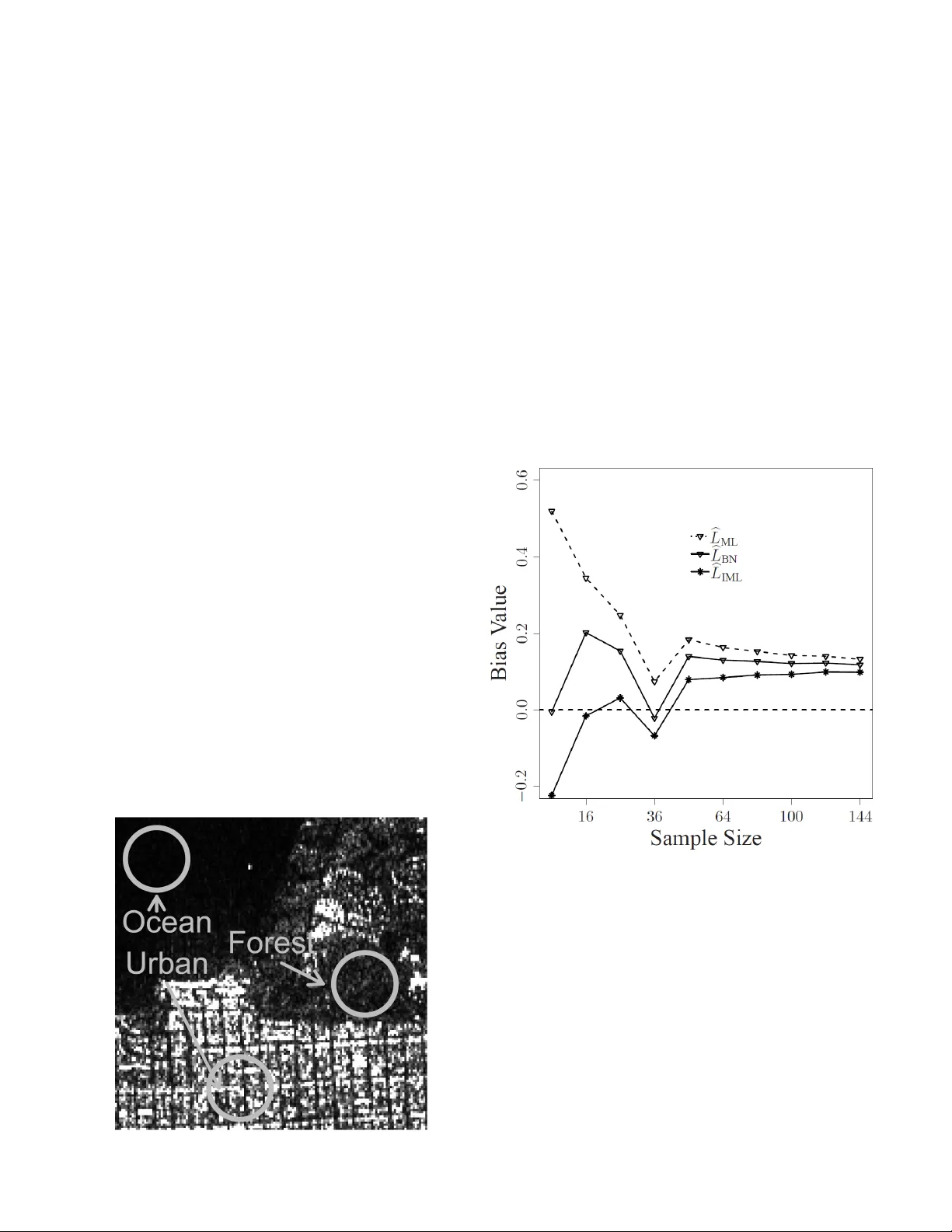
1 Bias Correction and Modified Profile Likelihood under the W ishart Comple x Distrib ution Abra ˜ ao D. C. Nascimento, Alejandro C. Frery , Senior Member , and Renato J. Cintra, Senior Member Abstract —This paper proposes impr oved methods f or the maximum likelihood (ML) estimation of the equiv alent number of looks L . This parameter has a meaningful interpr etation in the context of polarimetric synthetic aperture radar (PolSAR) images. Due to the presence of coherent illumination in their processing, PolSAR systems generate images which present a granular noise called speckle. As a potential solution for reducing such interference, the parameter L contr ols the signal-noise ratio. Thus, the proposal of efficient estimation methodologies for L has been sought. T o that end, we consider firstly that a PolSAR image is well described by the scaled complex Wishart distrib ution. In recent years, Anfinsen et al. derived and analyzed estimation methods based on the ML and on trace statistical moments for obtaining the parameter L of the unscaled version of such probability law . This paper generalizes that appr oach. W e present the second-order bias expr ession proposed by Cox and Snell for the ML estimator of this parameter . Moreover , the formula of the profile likelihood modified by Barndorff-Nielsen in terms of L is discussed. Such derivations yield two new ML estimators for the parameter L , which are compared to the estimators proposed by Anfinsen et al. . The perf ormance of these estimators is assessed by means of Monte Carlo experiments, adopting three statistical measures as comparison criterion: the mean square error , the bias, and the coefficient of variation. Equivalently to the simulation study , an application to actual PolSAR data concludes that the proposed estimators outperf orm all the others in homogeneous scenarios. I . I N T R O D U C T I O N Multilook polarimetric synthetic aperture radar (PolSAR) is a technology which has proven to be an effecti ve tool for geophysical remote sensing [1]. This particular system operates by sending electromagnetic pulses of several polar- izations tow ards a remote target; then the returning echoes are captured and registered. This process is characterized by the use of coherent illumination, which affects the obtained images with a granular noise called ‘speckle’. Therefore, a specialized modeling is required for processing and analyzing such images. In this context, the scaled complex Wishart distribution has been suggested as a successful approach for modeling the backscattered PolSAR signal. This distribution is equipped This work was supported by CNPq, Fapeal and F A CEPE, Brazil. A. D. C. Nascimento is with the Departamento de Estat ´ ıstica, Universidade Federal de Pernambuco, Cidade Universit ´ aria, 50740-540, Recife, PE, Brazil, e-mail: abraao.susej@gmail.com This work was partially funded by Conicet, CNPq, Fapeal and Capes. A. C. Frery is with the LaCCAN – Laborat ´ orio de Computac ¸ ˜ ao Cient ´ ıfica e An ´ alise Num ´ erica, Universidade Federal de Alagoas, BR 104 Norte km 97, 57072-970, Macei ´ o, AL, Brazil, e-mail: acfrery@gmail.com R. J. Cintra is with the Signal Processing Group, Departamento de Es- tat ´ ıstica, Univ ersidade Federal de Pernambuco, Cidade Universit ´ aria, 50740- 540, Recife, PE, Brazil, e-mail: rjdsc@ieee.org with two parameters: a cov ariance matrix and the number of looks ( L ). The former quantity is directly related to the data structure and is defined over the set of positiv e-definite Hermitian matrices [2]. On the other hand, parameter L is defined as the mean number of statistically independent samples represented by each pixel. Indeed, parameter L is related to the signal-to-noise ratio and the speckle noise is less se vere for large values of L [3], [4]. Sev eral studies hav e addressed the issue of estimating L [5], [6]. Despite the various existing approaches, the maximum likelihood (ML) method is often selected as the method of choice. This is mainly due to its good asymptotic properties, such as consistency and con ver gence in distribution to the Gaussian law [7]. Howe ver , the ML estimator in finite samples is usually biased with respect to the true parameter value. Indeed, the ML estimator bias has order O ( N − 1 ) , where N is the sample size and O ( · ) is Landau notation to represent order . In practice, this quantity is not commonly considered because its value is negligible when compared to the standard error , which has order O ( N − 1 / 2 ) . Howe ver , such biases can be substantial in situations where small or moderate sample sizes are used. Thus, analytic e xpressions for the ML estimator bias hav e been sought in order to derive a more accurate, corrected estimator for finite sample sizes [8], [9]. In [10], Cox and Snell proposed a general formula for the second-order bias of the ML estimator . Sev eral works hav e considered this formula as a mean to obtain improved estimators for parameters of several distributions [9]. V ascon- cellos et al. [8] applied it to the univ ariate G 0 distribution, which is often used for modeling synthetic aperture radar (SAR) images with one polarization channel [11]. Pianto and Cribari-Neto [12] proposed a bias correction approach for the roughness parameter of the G 0 distribution. More accurate ML estimators can also be deriv ed by means of the modified profile likelihood [13, chapter 9]. In this approach, an improved parameter estimation can be achieved by maximizing an adjusted profiled likelihood function [14]. Barndorff-Nielsen proposed a successful adjustment for the profile likelihood in [15]. This methodology could offer para- metric inference techniques suitable for se veral distributions. The Birnbaum-Saunders distribution [16] and elliptical struc- tural models [17] are illustrative examples. This approach has also been employed in SAR data models. Silva et al. [18] proposed point estimation and hypothesis test methods for the roughness parameter of the G 0 distribution based on modified profile likelihood. Anfinsen et al. [5] proposed three methods for estimating 2 the number of looks. Their methods were fav orably compared with classic methods based on fractional moment and the coefficient of variation. Assuming that PolSAR images are well modeled by the complex Wishart distribution, the ML estimator was found to excel when compared to other classic techniques. Additionally , such estimators were submitted to bias analysis by means of jackknife and bootstrap tech- niques [5]. Howe ver , these techniques are computationally intensiv e and are prone to inaccuracies when small sample sizes are considered [19]. The aim of this paper is three-fold. First, we derive a second-order bias expression for the ML estimator of param- eter L and propose corrected estimator for L following Cox- Snell approach [10]. Second, considering the scaled complex W ishart law , we propose a new estimator for L according Barndorff-Nielsen correction [15]. Third, the performance of the proposed corrected ML estimators is quantified and compared to the estimators listed in literature. This assessment is performed according to Monte Carlo experiments at sev eral different simulation scenarios. Actual PolSAR data are also considered and analyzed. The remainder of this paper is structured as follows. In Section II, we revie w the scaled complex Wishart distribution, which is the probability model considered in this work. Sec- tion III discusses Cox-Snell and Barndorff-Nielsen methodolo- gies for obtaining corrected ML estimators. In Section IV, the new corrected estimators are introduced and mathematically described. Subsequently , the deriv ed estimators are analyzed and compared with existing literature techniques in Section IV. Finally , conclusions are summarized in Section VI. I I . S C A L E D C O M P L E X W I S H A RT D I S T R I B U T I O N A N D M L E S T I M A T I O N A. Scaled Complex W ishart distribution The polarimetric coherent information associates to each image pixel a 2 × 2 comple x matrix. The entries of such matrix are S VV , S VH , S HV , and S HH , where S ij represents the backscattered signal for the i th transmission and j th reception linear polarization, for i, j = H , V. Under the reciprocity the- orem conditions [20], the scattering matrix is often simplified into a three-component vector , because S HV = S VH . Thus, we hav e the following scattering vector  S VV √ 2 S VH S HH  > , where the superscript > denotes vector transposition. This three-component representation is detailed in [21]. In general, we may consider a system with m polarizations. Thus the associated complex random vector is denoted by: s =  S 1 S 2 · · · S m  > , where S j , j = 1 , 2 , . . . , m , represents the random variables associated with each polarization channel. This particular ran- dom vector has been successfully modeled by the multi variate complex Gaussian distribution with zero-mean, as discussed in [22]. Thus, the single-look PolSAR data representation is essentially gi ven by s . Multilook polarimetric speckled data obtained from scat- tered signal is commonly defined by the estimated sample cov ariance matrix [5], which is giv en by Z = 1 L L X i =1 s i s H i , where the superscript H represents the complex conjugate transpose of a vector , s i , i = 1 , 2 , . . . , L , are scattering vectors, and L is the number of looks. Matrix Z is Hermitian positiv e definite and follo ws a scaled complex W ishart distri- bution [5]. Having Σ and L as parameters, the scaled complex W ishart distribution is associated to the following probability density function [2]: f Z ( Z 0 ; Σ , L ) = L mL | Z 0 | L − m | Σ | L Γ m ( L ) exp  − L tr( Σ − 1 Z 0 )  , where Γ m ( L ) = π m ( m − 1) / 2 Q m − 1 i =0 Γ( L − i ) for L ≥ m , Γ( · ) is the gamma function, tr( · ) represents the trace operator , | · | denotes the determinant operator , Σ is the cov ariance matrix associated to s , Σ = E  ss ∗  =      E( S 1 S ∗ 1 ) E( S 1 S ∗ 2 ) · · · E( S 1 S ∗ m ) E( S 2 S ∗ 1 ) E( S 2 S ∗ 2 ) · · · E( S 2 S ∗ m ) . . . . . . . . . . . . E( S m S ∗ 1 ) E( S m S ∗ 2 ) · · · E( S m S ∗ m )      , and superscript ∗ means the conjugate of a complex number . The first moment of Z satisfies E( Z ) = Σ [5], where E( · ) is the statistical expectation operator . W e denote Z ∼ W ( Σ , L ) to indicate that Z follows the scaled complex W ishart distri- bution. B. Estimation of Scaled Complex W ishart Distrib ution P aram- eters Let { Z 1 , Z 2 , . . . , Z N } be a random sample from Z ∼ W ( Σ , L ) . The ML estimators for Σ and L , namely b Σ ML and b L ML , respectiv ely , are quantities that maximize the log- likelihood function associated to the Wishart distribution, which is given by [5], [23]: ` ( θ ) = mN L log L + ( L − m ) N X k =1 log | Z k | − LN log | Σ | − N m ( m − 1) 2 log π − N m − 1 X k =0 log Γ( L − k ) − N L tr( Σ − 1 ¯ Z ) , (1) where ¯ Z = N − 1 P N k =1 Z k , θ =  σ > L  > , σ = v ec( Σ ) , and v ec( · ) is the column stacking vectorization operator . In a pre vious work [23], we have showed that b Σ ML is gi ven by the sample mean, b Σ ML = ¯ Z , 3 and b L ML satisfies the following non-linear equation: m log b L ML + 1 N N X k =1 log | Z k | − log | ¯ Z | − ψ (0) m ( b L ML ) = 0 , (2) where ψ (0) m ( · ) is the zeroth order term of the v th-order multi- variate polygamma function given by ψ ( v ) m ( L ) = m − 1 X i =0 ψ ( v ) ( L − i ) , ψ ( v ) ( · ) is the ordinary polygamma function expressed by ψ ( v ) ( L ) = ∂ v +1 log Γ( L ) ∂ L v +1 , for v ≥ 0 . Function ψ (0) ( · ) is kno wn as the digamma function. In abov e expression (2) a closed-form analytical solution for b L ML [5], [23] could not be identified. Ne vertheless, b L ML can be obtained via the Newton-Raphson numerical optimization method [24]. A detailed account on the performance of b L ML is provided in [5]. Howe ver , estimator b L ML is not adequate for applications based on small sample sizes, such as filtering methods for image restoration [25], [26]. This is due to the fact that the ML estimator is only guaranteed to be asymptotically unbiased; therefore, techniques which depend on ML estimates under small samples may suffer from pronounced bias. A con venient estimator based on the method of moments for the equi valent number of looks (ENL) was proposed in [27] and suggested for both single-polarization and PolSAR data [5]. Howe ver , for that particular method, in the PolSAR case, the cross-terms of the estimated sample covariance matrix are not considered [5], which means that potentially useful information is simply being discarded. T o address this issue, Anfinsen et al. [5] proposed two estimators based on trace moment, whose expressions are giv en by: b L MM1 = tr( ¯ Z ¯ Z ) N − 1 P N i =1 tr( Z i ) 2 − tr( ¯ Z ) 2 and b L MM2 = tr( ¯ Z ) 2 N − 1 P N i =1 tr( Z i Z i ) − tr( ¯ Z ¯ Z ) . These estimators are based on the deriv ations proposed by Maiwald and Kraus [28]. I I I . C O R R E C T E D M L E S T I M A T I O N M E T H O D S Sev eral works hav e addressed the ML estimator properties in finite sample for SAR data modeling [8], [12], [18]. ML estimation for other statistical models has also been proposed [9], [16], [17]. In this section, we describe two methodologies for obtaining improved ML estimators. The first one is based on the ML estimator second-order bias according to the Cox and Snell general formula [10]. The second method is based on the modified profile likelihood and was proposed by Barndorff-Nielsen [15]. A. Mathematical F ramework In this subsection, we present the mathematical framework required for both methods above referred to. Let { Z 1 , Z 2 , . . . , Z N } be a random sample from a random positiv e-definite Hermitian matrix Z equipped with a given density f Z ( Z 0 ; θ ) , where Z 0 represents possible outcomes and θ =  θ 1 θ 2 · · · θ p  > is the parameter vector with length p . The associated log-likelihood function based on above ob- servations is gi ven by ` ( θ ) = N X k =1 log f Z ( Z k ; θ ) . The deriv ativ es of the log-likelihood play an important role in ML estimation. For the sake of compactness, we adopt the following notation: U θ i = ∂ ∂ θ i ` ( θ ) , U θ i θ j = ∂ 2 ∂ θ i ∂ θ j ` ( θ ) , U θ i θ j θ k = ∂ 3 ∂ θ i ∂ θ j ∂ θ k ` ( θ ) , for i, j, k = 1 , 2 , . . . , p . Accordingly , we denote the cumulants for the log-likelihood deriv atives as [9]: κ θ i θ j = E( U θ i θ j ) , κ θ i ,θ j = E( U θ i U θ j ) , κ θ i θ j θ k = E( U θ i θ j θ k ) , κ θ i ,θ j θ k = E( U θ i U θ j θ k ) . As a direct consequence, the elements of the Fisher informa- tion matrix associated to θ are κ θ i ,θ j . Additionally , we denote the elements of the in verse of the Fisher information matrix as κ θ i ,θ j . Moreov er , the first deriv ati ve of the cumulants with respect to the parameters is denoted by: κ ( θ k ) θ i θ j = ∂ ∂ θ k κ θ i θ j , for i, j, k = 1 , 2 , . . . , p . B. Cox-Snell Corrected ML Estimator Let ˆ θ i , i = 1 , 2 , . . . , p , be the ML estimator for θ i . Considering the mathematical expressions described in the previous subsection, the Cox-Snell expression for the bias of ˆ θ i is described here. Such bias correction was given an alternativ e form in terms of the cumulants of the log-likelihood deriv ativ es [9]. It was established that the bias of ˆ θ i possesses the follo wing formulation [9]: B ( b θ i ) = E( b θ i ) − θ i = X r,s,t κ θ i ,θ r κ θ s ,θ t  κ ( θ t ) θ r θ s − 1 2 κ θ r θ s θ t  , (3) Therefore, the corrected ML estimator e θ i is defined by e θ i = b θ i − b B ( b θ i ) , (4) where b B ( b θ i ) represents the bias B ( b θ i ) ev aluated not at θ i but at b θ i . Additionally , it was pre viously sho wn that (i) E[ b B ( b θ i )] = 4 O  N − 2  , (ii) E( b θ i ) = θ i + O  N − 1  , and (iii) E( e θ i ) = θ i + O  N − 2  [10]. Therefore the bias of e θ i has order of N − 2 . In contrast, we hav e that B ( b θ i ) = O  N − 1  [8]. Thus, e θ i is expected to possess better asymptotic properties when compared to b θ i . C. Barndorff-Nielsen ML Estimator In [15] Barndorff-Nielsen introduced an improved ML esti- mation based on the modified profile likelihood. This method was previously employed in [16]–[18]. Below we furnish a brief outline of the technique. Let the parameter vector θ be split into two vectors such that θ =  ψ > λ >  > , where ψ and λ have q and p − q elements, respectiv ely . V ector ψ is the interest parameter vector , whereas vector λ is the nuisance parameter vector . In [29], [30], the statistical inference of ψ , for a known λ , was addressed. Howe ver , such calculation requires the marginal or condi- tional likelihood functions, which are often mathematically intractable [18]. A common solution to this conundrum is to approximate these functions by the profile log-likelihood [14], which is denoted by e ` ( ψ ) = `  ψ b λ ψ  , where b λ ψ is the maximum likelihood estimator of λ expressed in terms of the elements of ψ . Howe ver , such approximation may be problematic. In fact, the profile log-likelihood is not a bona fide log-likelihood function [15]. Moreov er , the associated profile score and the information biases are only guaranteed to be O (1) [31]. Therefore ML estimators based on profile log-likelihood are prone to bias issues, specially for small sample sizes [18]. T o address this issue, se veral modifications for the profile log-likelihood function have been proposed [15], [29], [30], [32]. In the current work, we adopted the Barndorff-Nielsen modification [15], which is analytically tractable when the scaled complex W ishart distribution is considered. Barndorff-Nielsen approximation for the mar ginal log- likelihood function is expressed according to [33]: e ` BN ( ψ ) = e ` ( ψ ) − log      ∂ b λ ψ ∂ b λ      − 1 2 log     J λλ  ψ b λ ψ      , (5) where b λ is the unrestricted maximum likelihood estimators for the nuisance parameter λ , and J λλ ( · ) is the observed information matrix for λ given by: J λλ  ψ b λ ψ  = − ∂ 2 ∂ λ ∂ λ H ` ( θ ) . The associated bias for e ` BN ( ψ ) is O ( N − 1 ) [33]. If b λ ψ = b λ for all ψ (i.e., ∂ b λ ψ /∂ b λ = I p − q , where I a represents a identity matrix with order a ), (5) collapses into: e ` BN ( ψ ) = e ` ( ψ ) − 1 2 log     J λλ  ψ b λ ψ      . (6) Abov e expression is known as the Cox-Reid modified profile log-likelihood [29]. The vector b ψ BN that maximizes (5) is the Barndorff-Nielsen ML estimator for ψ [18]. It is shown in [33] that the bias of b ψ BN is O ( N − 3 / 2 ) . Therefore, for this particular log-likelihood function, the ML estimator bias is also O ( N − 3 / 2 ) . This is an impro vement over the standard ML estimator, whose bias is O ( N − 1 ) . I V . I M P RO V E D M L E S T I M A T I O N F O R T H E S C A L E D C O M P L E X W I S H A RT D I S T R I B U T I O N In this section we propose improv ements to ML estimators for the parameters of the scaled complex Wishart distrib ution. W e consider the methodologies described in the pre vious section, namely the Cox-Snell corrected ML estimation and the Barndorff-Nielsen ML estimation based on the modified profile log-likelihood function. Mainly , our goal is to deriv e corrected ML estimators for Σ and L . Howe ver , as established in [23], we notice that E( b Σ ML ) = Σ . Therefore, b Σ ML is already unbiased, requiring no correction. Thus, we focus our ef forts on obtaining a corrected ML estimator for L . A. Cox-Snell Corrected ML estimators for Σ and L According to (4), the Cox-Snell method yields an improv ed ML estimator for L , termed by b L IML , gi ven by b L IML = b L ML − b B ( b L ML ) . (7) Now we aim at computing b B ( b L ML ) . For such firstly we need to derive B ( b L ML ) . In voking (3), we have that B ( b L ML ) = κ L,L κ L,L  κ ( L ) LL − 1 2 κ LLL  + m 2 X i =1 m 2 X j =1 κ L,L κ σ i ,σ j  κ ( σ i ) Lσ i − 1 2 κ Lσ i σ j  . (8) Follo wing algebraic manipulations, as detailed in Appendix A, we could simplify (8) and re-cast it as B ( L ) = m 2 2 N L h ψ (1) m ( L ) − m L i − m 2 L + ψ (2) m ( L ) 2 N h ψ (1) m ( L ) − m L i 2 . Now replacing L by b L ML , we obtain b B ( b L ML ) . This quan- tity must be inserted back into (7) to furnish the proposed improv ed ML estimator for L . B. Modified pr ofile log-likelihood for number of looks Follo wing the discussed Barndorff-Nielsen technique, we deriv e the profile log-likelihood function associated to the scaled complex Wishart distribution. This quantity can be obtained by replacing the cov ariance matrix Σ by its ML estimator b Σ ML in (1). This particular manipulation yields e ` ( · ) 5 as a function of the sought parameter L : e ` ( L ) = mN L (log L − 1) + ( L − m ) N X k =1 log | Z k | − N L log | ¯ Z | − N m ( m − 1) 2 log π − N m − 1 X k =0 log Γ( L − k ) . (9) Thus, the profile score function is giv en by e U ( L ) = ∂ e ` ( L ) ∂ L = mN log L − N ψ (0) m ( L ) − N log | ¯ Z | + N X k =1 log | Z k | . From (1), we could express the profile score function in terms of σ = vec( Σ ) , yielding: U ( σ ) = N v ec( Σ − 1 ¯ Z Σ − 1 − Σ − 1 ) . By imposing U ( σ ) = 0 , where 0 is a column vector of zeros, and solving the resulting system of equations, one obtains that the unrestricted and restricted ML estimators for σ are giv en by v ec( ¯ Z ) . Moreover , we hav e that ∂ b σ L ∂ b σ = I m 2 , where b σ L represents the restricted ML estimator . As a conse- quence, we are now in a position to use (6). Howe ver , the following quantity is necessary: − 1 2 log     J σ σ  L b σ      , where b σ = vec( b Σ ML ) . Due to its length, the mathematical deriv ation for this quantity is detailed in Appendix B. Thus, from (6), the modified profile log-likelihood according to the Barndorff-Nielsen technique is furnished by e ` BN ( L ) = e ` ( L ) − m 2 2 (log N + log L ) − m log | ¯ Z − 1 | . (10) As a consequence, the associated relativ e score function is expressed by e U BN ( L ) = ∂ ∂ L e ` BN ( L ) = e U ( L ) − m 2 2 L . As required, the sought estimator b L BN must satisfy e U BN ( b L BN ) = 0 . In other words, it is the solution of the following non-linear equation: mN log b L BN − N ψ (0) m ( b L BN ) − N log | ¯ Z | + N X k =1 log | Z k | − m 2 2 b L BN = 0 . (11) A closed-form e xpression for b L BN could not be gi ven. Then we resort to numerical techniques, such as the Ne wton-Raphson method, as a means for solving (11). V . P E R F O R M A N C E A N D A S S E S S M E N T T o assess the performance of the proposed estimators for the equiv alent number of looks, we considered a simulation study on synthetic data based on Monte Carlo experiments. Such simulation included the following estimators: 1) the standard ML estimator ( b L ML ) [5]; 2) the first and second trace moment estimators ( b L MM1 and b L MM2 , respecti vely) [5]; 3) the proposed ML estimator based on the Cox and Snell methodology ( b L IML ); and 4) the proposed ML estimator according to the Barndorff- Nielsen adjustment ( b L BN ). The first three above-mentioned estimators were derived by Anfinsen et al. [5]. Simulation results, were assessed in terms of three statistical measures: (i) the mean squared error (MSE); (ii) the coef ficient of variation (CV); and (iii) the mean estimated values; and (iv) the bias curves ( B ). Subsequently we separate the best estimator among those proposed by Anfinsen et al. as indicated by the simulation study . Then such selected estimator as well as the proposed estimators are submitted to actual data analysis aiming at performance assessment. A. Simulation study The suggested Monte Carlo simulation employed 5500 replications as discussed in [34]. Additionally , the following simulation parameters were considered: (i) sample sizes N ∈ { 9 , 49 , 121 } ; (ii) number of looks L ∈ { 4 , 6 , 8 , 12 } ; and (iii) a covariance matrix giv en by Σ 0 =   962892 19171 − 3579 i − 154638 + 191388 i 56707 − 5798 + 16812 i 472251   , where the omitted elements can be obtained from the conju- gation of their respectiv e symmetric elements. The adopted sample sizes are associated to square windows of { 3 , 7 , 11 } pixels, respectiv ely . It is worth mentioning that higher v alues of L represent images less af fected by speckle noise. This particular estimated cov ariance matrix Σ 0 was obtained by the E-SAR sensor ov er W eßling, Germany . In particular , it was employed in [35] for the characterization of urban areas. The results for MSE, CV , and mean estimated values are shown in T able I. Initially we notice that the proposed estimators b L BN and b L IML could of fer more accurate av erage ML estimates for the ENL when compared to the results deriv ed from the other considered methods. In general terms, the increasing of sample size reduces the MSE and CV . This behavior is expected, because the estimators are asymptot- ically unbiased. Results also show that the estimator b L IML presented the best performance in terms of MSE and CV in all considered cases. This last result provides even stronger evidence in fav or of the accuracy of b L IML . This is because bias corrected estimators do not al ways yield better procedures than ML estimators. Indeed, bias corrected estimators can offer 6 larger v ariance values, leading to increased MSE values when compared to uncorrected methods [9]. Fig. 1 presents the values of bias for sev eral sample sizes. The follo wing inequality is verified: b B ( b L MM1 ) ≥ b B ( b L MM2 ) ≥ b B ( b L ML ) ≥ b B ( b L BN ) ≥ b B ( b L IML ) . It is noteworth y that, with the exception of b L IML , all the pro- cedures o verestimate the equiv alent number of looks, i.e., they lead to decisions that assume that there is more information in the data than the true content. The only estimator with a different behavior is b L IML . It consistently exhibits the smallest bias, which is reduced with increasing number of looks. For large L and small samples, its bias becomes negati ve. The other estimators hav e their biases increased with the number of looks. The estimator b L IML was also less affected by the increasing of number of looks. Thus, this estimator performed well endur- ing both variations of the sample size as well as the number of looks. W e also emphasize that the better performance of estimator b L ML in comparison with b L MM1 and b L MM2 is in agreement with the findings of Anfisen et al. [5]. Ho wev er , when considering the proposed estimators, we identify that b L ML , b L IML , and b L BN as the more accurate estimators among the considered techniques. B. Analysis with actual data Now we aim at submitting actual PolSAR data to the three best estimators separated in the previous subsection. W e adopted the San Francisco AIRSAR image as a source of actual data. This classical multilook PolSAR image was obtained by the AIRSAR sensor operating at L band with four nominal looks [36]. Fig. 2 presents the HH channel intensity data of the 150 × 150 San Francisco image. Sub- areas were selected from the main image. By means of visual inspection, three categories were sought: (i) ocean; (ii) forest; and (iii) urban area. Fig. 2. San Francisco image with selected regions. For each selected subregion, we considered 5500 subsam- ples without replacement with size N ∈ { 9 , 36 , 121 , 144 } . These subsamples are then submitted to parameter estimation. T able II displays the obtained results. For the selected ocean subregion, the corrected estimator b L IML presented the smallest v alues of MSE and CV . Thus, the furnished estimates were more accurate. As discussed by Anfinsen et al. [5], tex- tured re gions yield to underestimation effects. Then correction schemes tend to become less efficient when compared to usual ML estimation b L ML . Indeed, as reported in [2], heavily textured images, such as forest and urban, are less adequately described by the com- plex W ishart distribution. This phenomenon was also verified in [37]–[39]. Therefore, the proposed tools are expected to excel at low textured samples. Fig. 3 shows the bias curves for the ocean region in which case the proposed tools were superior . These curves indicate that the estimator b L IML could outperform the usual ML estimator when homogeneous targets are considered. Fig. 3. Bias curves in terms of sample sizes for actual data. Finally , we notice that both T able II and Figure 3 indi- cate that the discussed estimators possess similar asymptotic properties. This behavior is expected and can deriv ed from theoretical results as shown in [7], [40]. V I . C O N C L U S I O N In this paper, we proposed two new improved corrected ML estimators for the scaled complex W ishart distribution. Emphasis was put on the estimation of the number of looks. In particular , we introduced closed-form expressions for the bias and for the modified profile likelihood according to methodologies advanced by Cox and Snell [10] and Barndorff- Nielsen [15]. 7 (a) L = 4 (b) L = 6 (c) L = 8 (d) L = 12 Fig. 1. Bias curves in terms of sample sizes for synthetic data. 8 T ABLE I M E AS U R E S O F T H E E S T IM ATO R S P E RF O R M AN C E W I T H S Y N T HE T I C DAT A L = 4 L = 6 L = 8 L = 12 b L N mean( b L ) MSE CV mean( b L ) MSE CV mean( b L ) MSE CV mean( b L ) MSE CV b L ML 9 4.339 0.414 0.126 6.663 1.373 0.145 8.967 2.810 0.153 13.538 6.963 0.158 b L MM1 6.278 23.174 0.676 9.344 52.605 0.689 12.478 95.978 0.698 18.119 190.432 0.683 b L MM2 4.957 2.993 0.291 7.401 6.399 0.285 9.849 11.800 0.294 14.606 24.977 0.292 b L IML 3.998 0.221 0.118 6.000 0.695 0.139 7.989 1.398 0.148 11.937 3.435 0.155 b L BN 4.090 0.243 0.118 6.150 0.760 0.140 8.197 1.518 0.148 12.259 3.700 0.155 49 4.055 0.042 0.049 6.110 0.133 0.057 8.157 0.258 0.059 12.269 0.661 0.063 4.333 1.045 0.223 6.452 2.201 0.219 8.601 3.809 0.216 12.847 8.363 0.215 4.165 0.294 0.124 6.235 0.633 0.122 8.313 1.093 0.120 12.435 2.388 0.119 4.000 0.037 0.048 6.002 0.115 0.056 7.998 0.222 0.059 12.007 0.559 0.062 4.014 0.037 0.048 6.026 0.117 0.057 8.031 0.225 0.059 12.059 0.568 0.062 121 4.023 0.016 0.031 6.041 0.048 0.036 8.064 0.096 0.038 12.100 0.237 0.039 4.131 0.350 0.140 6.182 0.738 0.136 8.212 1.261 0.134 12.310 2.820 0.134 4.063 0.108 0.080 6.097 0.233 0.077 8.113 0.403 0.077 12.164 0.871 0.076 4.001 0.015 0.031 5.998 0.045 0.035 8.001 0.090 0.038 11.995 0.222 0.039 4.006 0.015 0.031 6.008 0.045 0.035 8.014 0.091 0.038 12.016 0.223 0.039 T ABLE II M E AS U R E S O F T H E E S T IM ATO R S P E RF O R M AN C E W I T H A C TU AL DAT A b L ML b L IML b L BN Regions N mean( b L ) MSE CV mean( b L ) MSE CV mean( b L ) MSE CV Ocean 9 4.520 0.747 0.153 3.776 0.350 0.145 3.995 1.376 0.294 36 4.074 0.623 0.193 3.932 0.582 0.193 3.979 0.739 0.216 121 4.140 0.034 0.029 4.099 0.024 0.029 4.123 0.029 0.029 144 4.133 0.029 0.026 4.099 0.021 0.025 4.118 0.025 0.026 Forest 3.293 0.599 0.095 3.069 0.938 0.087 3.159 0.792 0.092 3.119 0.794 0.043 3.075 0.872 0.042 3.089 0.852 0.049 2.809 2.041 0.281 2.798 2.065 0.281 2.818 1.987 0.273 3.082 0.845 0.017 3.072 0.864 0.017 3.075 0.858 0.017 Urban 2.738 2.439 0.336 2.492 3.239 0.394 2.678 2.451 0.313 2.567 2.486 0.256 2.529 2.594 0.260 2.454 2.989 0.316 2.218 3.959 0.399 2.209 3.990 0.401 2.177 4.146 0.417 2.447 2.833 0.265 2.439 2.857 0.265 2.426 2.923 0.275 By means of Monte Carlo simulations, the proposed tech- niques were assessed and compared with estimators presented by Anfinsen et al. [5]. Adopted figures of merit include MSE, coefficient of v ariation, mean of estimated v alues, and the bias curves. Results showed that the proposed corrected estimators outperform all considered estimators. Actual data were also analyzed rev ealing that the proposed estimators are superior when homogeneous scenes are considered. A P P E N D I X A C U M U L A N T S F O R T H E C OX - S N E L L C O R R E C T I O N In this appendix, we present closed-form expressions for (i) some cumulants from the scaled complex Wishart distri- bution as well as (ii) the second-order bias according to the Cox-Snell approach. From (1), the second and third-order deriv atives are gi ven by U LL = N m L − N ψ (1) m ( L ) , (12) U Lσ i = N [v ec( Σ − 1 ¯ Z Σ − 1 − Σ − 1 )] i , (13) U σ i σ j = LN [( Σ − 1 ⊗ Σ − 1 ) − ( Σ − 1 ⊗ Σ − 1 ) ¯ Z Σ − 1 − ( Σ − 1 ⊗ Σ − 1 ) Σ − 1 ¯ Z ] i, j , (14) U Lσ i σ j = L − 1 U σ i σ j , U σ i σ j σ k = LN [3( Σ − 1 ⊗ Σ − 1 ) ⊗ ( Σ − 1 ¯ Z Σ − 1 ) + 3( Σ − 1 ⊗ Σ − 1 ) ⊗ ( Σ − 1 Σ − 1 ¯ Z ) − 2( Σ − 1 ⊗ Σ − 1 ) ⊗ Σ − 1 ] k +( i − 1) m 2 , k +( j − 1) m 2 , for i, k , j = 1 , 2 , . . . , m 2 , where ⊗ is the Kronecker product and σ i is the i th element of vector σ . Based on the abov e results, we deriv e the following expres- sion for the cumulants: 9 κ L,L = 1 N  ψ (1) m ( L ) − m L  − 1 , κ L,σ i = 0 , κ σ i ,σ j = 1 N L ( Σ ⊗ Σ ) i, j , κ LLL = κ ( L ) LL = − N h m L 2 + ψ (2) m ( L ) i , κ LLσ i = κ ( σ i ) LL = κ ( σ j ) Lσ i = 0 , (15) κ σ i σ j L = − N ( Σ − 1 ⊗ Σ − 1 ) i, j , κ ( σ k ) σ i σ j = 2 LN [( Σ − 1 ⊗ Σ − 1 ) ⊗ Σ − 1 ] k +( i − 1) m 2 , k +( j − 1) m 2 , κ σ i σ j σ k = 4 LN [( Σ − 1 ⊗ Σ − 1 ) ⊗ Σ − 1 ] k +( i − 1) m 2 , k +( j − 1) m 2 . Since κ Lσ i = 0 , parameters L and σ i , for i = 1 , 2 , . . . , m 2 , are orthogonal [41]. Therefore, expression (3) yields: B ( b L ML ) = κ L,L κ L,L  κ ( L ) LL − 1 2 κ LLL  + m 2 X i =1 m 2 X j =1 κ L,L κ σ i ,σ j  κ ( σ i ) Lσ i − 1 2 κ Lσ i σ j  . Abov e formula can be gi ven a closed form expression. Indeed, from (15), we have that κ σ i ,σ j  κ ( σ i ) Lσ i − 1 2 κ Lσ i σ j  = 1 N L ( Σ ⊗ Σ ) i, j  0 + N 2 { Σ − 1 ⊗ Σ − 1 } i, j  = 1 2 L ( Σ ⊗ Σ ) i, j { ( Σ ⊗ Σ ) − 1 } i, j . Considering the general expression of the elements of the in verse matrix [42, pp. 82], we have: m 2 X i =1 m 2 X j =1 { Σ ⊗ Σ } i, j { ( Σ ⊗ Σ ) − 1 } i, j = m 2 . Therefore, we obtain: B ( b L ML ) = m 2 2 N L  ψ (1) m ( L ) − m L  − m 2 L + ψ (2) m ( L ) 2 N  ψ (1) m ( L ) − m L  2 . A P P E N D I X B D E R I V A T I O N F O R B A R N D O R FF - N I E L S E N A P P R OX I M A T I O N In the subsequent discussion, we aim to detail the deriv ation of the Barndorf f-Nielsen approximation for the marginal log- likelihood function of the scaled complex Wishart distribution. In particular, this appendix addresses the deri vation for the quantity − 1 2 log     J σ σ  L b σ      discussed in Subsection IV -B. Based on results (12)-(14), one can re write the observed in- formation matrix from the scaled complex W ishart distribution by the following matrix equation: " U LL U > L vec( Σ ) U vec( Σ ) ∗ L U vec( Σ ) v ec( Σ ) ∗ # = " mN L − N ψ (1) m ( L ) N vec( Σ − 1 ¯ Z Σ − 1 − Σ − 1 ) > N vec( Σ − 1 ¯ Z Σ − 1 − Σ − 1 ) ∗ U vec( Σ ) v ec( Σ ) ∗ # , where U > L vec( Σ ) , defined by U > L vec( Σ ) = ∂ 2 ∂ L∂ v ec( Σ ) > ` ( θ ) , is a vector whose the i th-element is given in (13) and [5] U vec( Σ ) v ec( Σ ) ∗ = ∂ 2 ∂ vec( Σ ) ∗ ∂ vec( Σ ) > ` ( θ ) = LN [( Σ − 1 ⊗ Σ − 1 ) − ( Σ − 1 ⊗ Σ − 1 ) ¯ Z Σ − 1 − ( Σ − 1 ⊗ Σ − 1 ) Σ − 1 ¯ Z ] . Thus, the quantity J σ σ  L b σ  can be defined by J σ σ  L b σ  = − U vec( Σ ) v ec( Σ ) ∗    Σ = ¯ Z = N L ¯ Z − 1 ⊗ ¯ Z − 1 . and, therefore, the following quantity combined with profile log-likelihood (9) at (6) yields the Barndorff-Nielsen approx- imation for the marginal log-likelihood function: − 1 2 log     J σ σ  L b σ      = − m 2 2 (log N + log L ) − 1 2 log   ¯ Z − 1 ⊗ ¯ Z − 1   . (16) From [43, result 11.1 (l), page 235], we hav e that log   ¯ Z − 1 ⊗ ¯ Z − 1   = 2 m log | ¯ Z − 1 | . Thus, (16) can be simplified according to: − 1 2 log     J σ σ  L b σ      = − m 2 2 (log N + log L ) − m log | ¯ Z − 1 | . Thus, we have that (10) holds true. R E F E R E N C E S [1] J. S. Lee and E. Pottier, P olarimetric Radar Imaging: Fr om Basics to Applications . Boca Raton: CRC, 2009. [2] C. C. Freitas, A. C. Frery , and A. H. Correia, “The polarimetric G distribution for SAR data analysis, ” Envir onmetrics , vol. 16, no. 1, pp. 13–31, 2005. [3] A. C. Frery , A. D. C. Nascimento, and R. J. Cintra, “ Analytic expressions for stochastic distances between relaxed complex Wishart distributions, ” IEEE Tr ansactions on Geoscience and Remote Sensing , in press-. [Online]. A v ailable: http://tiny .tw/3aIN [4] A. D. C. Nascimento, M. M. Horta, A. C. Frery , and R. J. Cintra, “Comparing edge detection methods based on stochastic entropies and distances for polsar imagery , ” IEEE Journal of Selected T opics in Applied Earth Observations and Remote Sensing , in press. [Online]. A vailable: http://tiny .tw/3aIP [5] S. N. Anfinsen, A. P . Doulgeris, and T . Eltoft, “Estimation of the equiv- alent number of looks in polarimetric synthetic aperture radar imagery , ” IEEE T ransactions on Geoscience and Remote Sensing , vol. 47, pp. 3795–3809, Nov . 2009. [6] C. H. Gierull and I. C. Sikaneta, “Estimating the effecti ve number of looks in interferometric SAR data, ” IEEE T ransactions on Geoscience and Remote Sensing , v ol. 40, pp. 1733–1742, Aug. 2002. [7] G. Casella and R. L. Berger , Statistical Infer ence . Duxbury Press, 2002. [8] K. L. P . V asconcellos, A. C. Frery , and L. B. Silva, “Improving estimation in speckled imagery , ” Computational Statistics , vol. 20, no. 3, pp. 503–519, 2005. 10 [9] G. M. Cordeiro, “Bias correction, ” in International Encyclopedia of Statistical Science , M. Lovric, Ed. Springer Berlin Heidelberg, 2011, pp. 148–152. [10] D. R. Cox and E. J. Snell, “A general definition of residuals, ” Journal of the Royal Statistical Society . Series B (Methodological) , v ol. 30, no. 2, pp. 248–275, 1968. [11] A. C. Frery , H. J. Muller , C. C. F . Y anasse, and S. J. S. Sant’Anna, “ A model for extremely heterogeneous clutter, ” IEEE Tr ansactions on Geoscience and Remote Sensing , vol. 35, pp. 648–659, May 1997. [12] D. M. Pianto and F . Cribari-Neto, “Dealing with monotone likelihood in a model for speckled data, ” Computational Statistics & Data Analysis , vol. 55, no. 3, pp. 1394 –1409, 2011. [13] T . A. Sev erini, Likelihood Methods in Statistics . Oxford Univ ersity Press, 2000. [14] D. A. S. Fraser and N. Reid, “ Adjustments to profile likelihood, ” Biometrika , vol. 76, no. 3, pp. 477–488, 1989. [15] O. E. Barndorff-Nielsen, “ Adjusted versions of profile likelihood and directed likelihood, and extended likelihood, ” Journal of the Royal Statistical Society . Series B (Methodological) , vol. 56, no. 1, pp. 125– 140, 1994. [16] A. H. M. A. Cysneiros, F . Cribari-Neto, and C. A. G. Ara ´ ujo Jr ., “On Birnbaum-Saunders inference, ” Computational Statistics & Data Analysis , vol. 52, no. 11, pp. 4939–4950, 2008. [17] T . Melo and S. Ferrari, “ A modified signed likelihood ratio test in elliptical structural models, ” AStA Advances in Statistical Analysis , vol. 94, pp. 75–87, 2010. [18] M. Silva, F . Cribari-Neto, and A. C. Frery , “Improved likelihood inference for the roughness parameter of the GA0 distribution, ” En- vir onmetrics , vol. 19, no. 4, pp. 347–368, 2008. [19] A. C. Frery , F . Cribari-Neto, and M. O. Souza, “ Analysis of minute features in speckled imagery with maximum likelihood estimation, ” EURASIP Journal on Advances in Signal Processing , vol. 2004, no. 16, pp. 2476–2491, 2004. [20] F . T . Ulaby and C. Elachi, Radar P olarimetriy for Geoscience Applica- tions . Norwood: Artech House, 1990. [21] A. Freeman and S. L. Durden, “ A three-component scattering model for polarimetric SAR data, ” IEEE Tr ansactions on Geoscience and Remote Sensing , vol. 36, pp. 963–973, May 1998. [22] N. R. Goodman, “Statistical analysis based on a certain complex Gaussian distribution (an introduction), ” The Annals of Mathematical Statistics , vol. 34, pp. 152–177, 1963. [23] A. C. Frery , R. J. Cintra, and A. D. C. Nascimento, “Entropy-based statistical analysis of PolSAR data, ” IEEE T ransactions on Geoscience and Remote Sensing , v ol. 51, pp. 3733–3743, Jun. 2013. [24] J. E. Gentle, Elements of Computational Statistics , ser . Statistics and computing. Springer , 2002. [25] A. Restrepo and A. C. Bovik, “ Adaptive trimmed mean filters for image restoration, ” IEEE T ransactions on Acoustics, Speech and Signal Pr ocessing , vol. 36, pp. 1326 –1337, Aug. 1988. [26] L. T orres, S. J. S. Sant’Anna, C. C. Freitas, and A. C. Frery , “Speckle reduction in polarimetric SAR imagery with stochastic distances and nonlocal means, ” P attern Recognition , in press. [Online]. A vailable: http://tiny .tw/3aIE [27] C. Oliver and S. Quegan, Understanding Synthetic Aperture Radar Images , ser . The SciT ech Radar and Defense series. SciT ech Publishing, 1998. [28] D. Maiwald and D. Kraus, “Calculation of moments of complex Wishart and complex inv erse Wishart distributed matrices, ” IEE Proceedings - Radar , Sonar and Navigation , vol. 147, pp. 162–168, Aug. 2000. [29] D. R. Cox and N. Reid, “ A note on the dif ference between profile and modified profile likelihood, ” Biometrika , vol. 79, no. 2, pp. 408–411, 1992. [30] S. E. Stern, “ A second-order adjustment to the profile likelihood in the case of a multidimensional parameter of interest, ” J ournal of the Royal Statistical Society . Series B (Statistical Methodology) , vol. 59, no. 3, pp. 653–665, 1997. [31] T . A. Severini, “Likelihood functions for inference in the presence of a nuisance parameter, ” Biometrika , vol. 85, no. 3, pp. 507–522, 1998. [32] P . McCullagh and R. T ibshirani, “A simple method for the adjustment of profile likelihoods, ” Journal of the Royal Statistical Society . Series B (Methodological) , vol. 52, no. 2, pp. 325–344, 1990. [33] O. E. Barndorff-Nielsen, “On a formula for the distribution of the maximum likelihood estimator, ” Biometrika , vol. 70, no. 2, pp. 343– 365, 1983. [34] A. D. C. Nascimento, R. J. Cintra, and A. C. Frery , “Hypothesis testing in speckled data with stochastic distances, ” IEEE T ransactions on Geoscience and Remote Sensing , vol. 48, pp. 373–385, Jan. 2010. [35] A. C. Frery , J. Jacobo-Berlles, J. Gambini, and M. Mejail, “Polarimetric SAR image segmentation with B-splines and a new statistical model, ” Multidimensional Systems and Signal Processing , vol. 21, pp. 319–342, 2010. [36] European Space Agency, P olarimetric SAR Data Processing and Educational T ool (P olSARpr o) , 4th ed. European Space Agency , 2009. [Online]. A vailable: http://earth.esa.int/polsarpro/ [37] A. C. Frery , A. H. Correia, and C. C. Freitas, “Classifying multifre- quency fully polarimetric imagery with multiple sources of statistical evidence and contextual information, ” IEEE T ransactions on Geoscience and Remote Sensing , v ol. 45, pp. 3098–3109, Oct. 2007. [38] L. Bombrun and J. M. Beaulieu, “Fisher distrib ution for texture modeling of polarimetric SAR data, ” IEEE Geoscience and Remote Sensing Letters , vol. 5, pp. 512–516, Jul. 2008. [39] L. Bombrun, G. V asile, M. Gay , and F . T otir , “Hierarchical segmentation of polarimetric SAR images using heterogeneous clutter models, ” IEEE T ransactions on Geoscience and Remote Sensing , vol. 49, pp. 726 –737, Feb . 2011. [40] S. M. Kay , Fundamentals of Statistical Signal Pr ocessing, V olume 1: Estimation Theory . Pearson Education, 1998. [41] D. R. Cox and N. Reid, “Parameter orthogonality and approximate conditional inference, ” Journal of the Royal Statistical Society . Series B (Methodological) , vol. 49, no. 1, pp. 1–39, 1987. [42] R. A. Johnson and D. W . W ichern, Applied Multivariate Statistical Analysis , ser. Prentice-Hall series in statistics. Prentice-Hall, 1988. [43] G. A. F . Seber , A Matrix Handbook for Statisticians , 1st ed. New Y ork, NY , USA: W iley-Interscience, 2007. Abra ˜ ao D. C. Nascimento holds B.Sc. M.Sc. and D.Sc. degrees in Statistics from Univ ersidade Federal de Pernambuco (UFPE), Brazil, in 2005, 2007, and 2012, respectiv ely . In 2013, he joined the Department of Statistics at UFPB as Adjoint Professor . His research interests are statistical infor- mation theory , inference on random matrices, and asymptotic theory . Alejandro C. Frery (S’92–SM’03) receiv ed the B.Sc. degree in Electronic and Electrical Engineer- ing from the Universidad de Mendoza, Mendoza, Argentina. His M.Sc. degree was in Applied Mathe- matics (Statistics) from the Instituto de Matem ´ atica Pura e Aplicada (IMP A, Rio de Janeiro) and his Ph.D. degree was in Applied Computing from the Instituto Nacional de Pesquisas Espaciais (INPE, S ˜ ao Jos ´ e dos Campos, Brazil). He is currently the leader of LaCCAN – Laborat ´ orio de Computac ¸ ˜ ao Cient ´ ıfica e An ´ alise Num ´ erica , Universidade Federal de Alagoas, Macei ´ o, Brazil. His research interests are statistical computing and stochastic modelling. Renato J. Cintra (SM’10) earned his B.Sc., M.Sc., and D.Sc. degrees in Electrical Engineering from Univ ersidade Federal de Pernambuco, Brazil, in 1999, 2001, and 2005, respectiv ely . In 2005, he joined the Department of Statistics at UFPE. During 2008-2009, he worked at the University of Calgary , Canada, as a visiting research fello w . He is also a graduate faculty member of the Department of Electrical and Computer Engineering, Uni versity of Akron, OH. His long term topics of research include theory and methods for digital signal processing, communications systems, and applied mathematics.