Random Binary Mappings for Kernel Learning and Efficient SVM

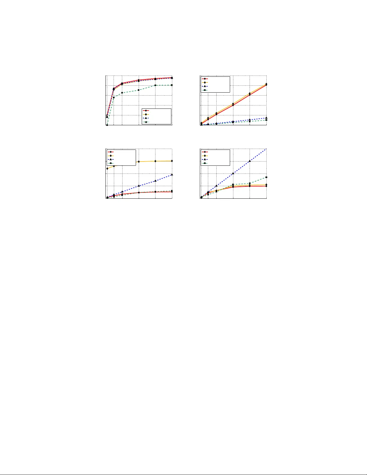
Random Decision Stumps f or K ernel Lear ning and Efficient SVM Gemma Roig * Xavier Boix * Luc V an Gool Computer V ision Lab, ETH Zurich, Switzerland { boxavier,gemmar,vangool } @vision.ee.ethz.ch * Both first authors contrib uted equally . Abstract. W e propose to learn the kernel of an SVM as the weighted sum of a large number of simple, randomized binary stumps. Each stump takes one of the extracted features as input. This leads to an efficient and very fast SVM, while also alleviating the task of kernel selection. W e demonstrate the capabilities of our kernel on 6 standard vision benchmarks, in which we combine sev eral com- mon image descriptors, namely histograms (Flowers17 and Daimler), attribute- like descriptors (UCI, OSR, and a-V OC08), and Sparse Quantization (ImageNet). Results sho w that our kernel learning adapts well to these different feature types, achieving the performance of kernels specifically tuned for each, and with an ev aluation cost similar to that of ef ficient SVM methods. 1 Introduction The success of Support V ector Machines (SVMs), e.g . in object recognition, stems from their well-studied optimization and their use of k ernels to solv e non-linear classification problems.Designing the right kernel in combination with appropriate image descriptors is crucial. Their joint design leads to a chic ken-and-e gg problem in that the right kernel depends on the image descriptors, while the image descriptors are designed for familiar kernels. Multiple K ernel Learning (MKL) [1] eases kernel selection by automatically learn- ing it as a combination of giv en base kernels. Although MKL has been successful in var - ious vision tasks ( e .g. [2,3]), it might lead to comple x and inefficient kernels. Recently , Bazav an et al. [4] introduced an approach to MKL that a v oids the explicit computation of the kernel. It efficiently approximates the non-linear mapping of the hand-selected kernels [5,6,7], thus deli vering impressi ve speed-ups. W e propose another way around kernel learning that also allows for efficient SVMs. Instead of combining fixed base kernels, we inv estigate the use of random binary map- pings (BMs). W e coin our approach Multiple Binary Kernel Learning (MBKL). Given that other methods based on binary decisions such as Random Forests [8] and Boosting decision stumps [9] hav e not performed equally well on image classification bench- marks as kernel SVMs, it is all the more important that we will show MBKL does. Not only does MBKL alleviate the task of selecting the right k ernel, b ut the resulting kernel is very ef ficient to compute and can scale to large datasets. At the end of the paper , we report on MBKL results for 6 computer vision bench- marks, in which we combine sev eral common image descriptors. These descriptors 2 Gemma Roig, Xavier Boix, Luc V an Gool are histogram-based (Flowers17 [10] and Daimler [11]), attribute-based (OSR [12], a-P ASCAL V OC08 detection [13], and UCI [14]), and Sparse Quantization [15] (Ima- geNet [16]). W e demonstrate for the first time that a classifier based on BMs can achie ve performances comparable to those of the hand-selected kernels for each specific de- scriptor . Moreover , it is as fast as the fastest kernel approximations, but without the need of interactiv ely selecting the kernel. 2 Efficient SVM and K ernel Lear ning In this section, we revisit the SVM literature, with special emphasis on efficient and scalable kernel learning for object recognition. Efficient SVM. W e use ( w , b ) to denote the parameters of the SVM model, and φ ( x ) for the non-linear mapping to a higher-dimensional space. The classification score for a feature vector x then is w T φ ( x ) + b . The SVM aims at minimizing the hinge loss. For the SVM implementation, one typically applies the kernel trick: with Lagrange multipliers { α i } the classification score becomes w T φ ( x ) + b = P i α i y i  φ ( x ) T φ ( x i )  + b = P i α i y i K ( x , x i ) + b (1) where K ( x , x i ) : R n × R n → R . The optimal multipliers α i tend to be sparse and select relati vely few ‘support vectors’ from the many training samples. The kernel trick bypasses the computation of the non-linear mapping by directly computing the inner products K ( x , x i ) . The strength of SVMs is that they yield max-margin classifiers. At test time, the computational cost is the number of support vectors times the cost of computing the kernel. The problem is that the latter may be quite expensi ve. Also, during training, the complexity of computing the kernel matrix grows quadratically with the number of training images, which renders it intractable for large datasets. Sev eral authors hav e tried to speed up kernel-based classification. Ideas include lim- iting the number of support vectors [17,18] or creating low-rank approximations of the kernel matrix [19]. These methods are ef fectiv e, but do not scale well to large datasets because they require the kernel distances to the training set. Rahimi and Recht intro- duced Random Fourier Features [6], thereby circumventing the approximation of the explicit feature map, φ ( x ) . Such techniques have been explored further for kernels used with common image descriptors, such as χ 2 and RB- χ 2 kernels [5,7] or the intersection kernel [20,21]. Other approaches use k ernel PCA to linearize the image descriptors [22] or sparse feature embeddings [23]. Recently , W u [24] introduced the po wer mean ker - nel, which generalizes the intersection and χ 2 kernels, among others, and achie ves a remarkably efficient, scalable SVM optimization. These methods approximate specific families of kernels. Our aim is to learn a fast kernel, which eases kernel selection, rather than approximating predefined k ernels. Random Decision Stumps for Kernel Learning and Ef ficient SVM 3 Multiple Kernel Learning (MKL). MKL [1] aims at jointly learning the SVM and a linear combination of giv en base kernels. The hope is that such committee of base kernels is a more powerful kernel. Denoting the base kernels as ˆ K , the final kernel K takes the form K ( x , x i ) = X k θ k ˆ K k ( x , x i ) , (2) where the weights θ k ∈ R + can be discriminativ ely learned. There have also been some approaches to find non-linear combinations of kernels, e.g . . [25,26], that we do not further consider here. In recent years, many advances ha ve been made to improv e the efficiency of MKL, and various optimization techniques have been introduced, e.g. semi-definite program- ming [27], SMO [1,28], semi-infinite linear programming [29] and gradient-based meth- ods [30,26]. Y et, scalability to lar ge datasets remains an issue, as these methods explic- itly compute the base kernel matrices. Therefore, Baza van et al. [4] exploit Random Fourier Features, which approximate the non-linear mapping of the kernel, and allow to scale to large datasets. Our approach is related to the latter in that it also aims at ef ficient and scalable kernel learning. Y et, MBKL ’ s base kernels are not hand-selected. Instead of approx- imating a distance coming with a pre-selected kernel, we explore the use of random BMs to learn a distance for classification. Indeed, in large-scale image retriev al, there is an increasing body of evidence that suggests that BMs are ef fectiv e to ev aluate dis- tances, e.g . [31,32,33]. In the next section, we introduce our formulation for kernel learning built from BMs. This, in turn, will yield a kernel very efficient to learn and to e valuate (Section 3). Moreov er , the kernel will adapt to most image descriptors, since it is learned from the input data (Section 5). 3 Multiple Binary K ernel Lear ning In this section, we introduce a kernel that is a linear combination of binary kernels, defined from a set of simple decision stumps. MKL with Binary Base Ker nels. BMs ha ve been used to speed-up distance computa- tions in large-scale image retrie v al, e.g. [31,32,33]. In these methods, the input feature is transformed into a binary vector that preserves the locality of the original feature space. In the context of classification, we can further enforce that the kernel in an SVM separates the image classes well. W e adopt the MKL formulation (see eq. (2)) as starting point of our kernel, since it aims at jointly learning the classifier and the kernel distance, yet incorporate BMs and restrict the base kernels to only take on binary v alues. The binary base kernels are defined as: ˆ K k ( x , x i ) = I [ σ k ( x ) = σ k ( x i )] , (3) 4 Gemma Roig, Xavier Boix, Luc V an Gool where I [ · ] is the indicator function, which returns 1 if the input is true and 0 otherwise, and σ k ( x ) is a BM of the input feature, σ k ( x ) : R n → { 0 , 1 } . Each base kernel is built upon one single BM. The BMs need not be linear and can be adapted to each problem if desired. In the sequel, we e xplore dif ferent possibilities, b ut our kernel is not restricted to any of them. In all cases, σ k ( x ) divides the feature space into tw o sets and the indicator function returns whether the two input samples fall in the same part of the feature space or not. The final kernel, K , is a linear combination of the binary kernels: K ( x , x i ) = P k θ k I [ σ k ( x ) = σ k ( x i )] . Note that K is not restricted to be binary , though the base kernels are. In the supplementary material we show that such ‘Multiple Binary K ernel’ (MBK) is a v alid Mercer kernel. An appropriate choice of the σ k ( x ) will be important to arrive at good classifications. For instance, in a two class problem, the better the set of σ k ( x ) separate the two classes, the better the kernel might be. Explicit Non-linear Mapping. W e analyze the form of the non-linear mapping of MBKL. In the Supplementary Material, we derive the non-linear mapping φ ( x ) that induces the MBKL kernel, and it is [ p θ 1 σ 1 ( x ) , p θ 1 ¯ σ 1 ( x ) , p θ 2 σ 2 ( x ) , p θ 2 ¯ σ 2 ( x ) , . . . ] T , (4) where ¯ σ k ( x ) is σ k ( x ) plus the not operation, and the SVM parameters are w T = [ p θ 1 c 1 1 , p θ 1 c 0 1 , p θ 2 c 1 2 , p θ 2 c 0 2 , . . . ] , (5) where c 1 k , c 0 k ∈ R are two learned constants, which correspond to the underlying pa- rameters of the classifier . W e can see that this mapping recov ers the MBKL kernel in the form φ ( x ) T φ ( x i ) . Thus, to e v aluate MBKL at test time, we do not need to e valuate the kernel because we ha ve access to the non-linear mapping φ . Benefits of kernel learning . MBKL generalizes a SVM with BMs as input features. This can be easily seen by fixing θ = 1 in eq. (4) and (5). But learning θ rather than fixing it to 1 has sev eral adv antages. Recall that the k ernel distance does not depend on the image class we are ev aluating. A BM with θ k equal to 0 does not contrib ute to the final kernel distance, and hence, can be discarded for all image classes. This is crucial to arri ve at a competiti ve computational comple xity . Moreov er , MBKL aims at learning a kernel distance adapted to the image descriptors, that can be used for tasks other than classification. MBKL is not a particular instance of any of the kernels in the literature. Rather the opposite may be true, since most kernels can be approximated with a collection of BMs [31]. 4 BMs as Random Decision Stumps W e found that defining the σ k ( x ) as simple random decision stumps achiev es excellent results with the image descriptors commonly used in the literature. Decision stumps select a component in a feature vector and threshold it. W e randomly select a component Random Decision Stumps for Kernel Learning and Ef ficient SVM 5 0 0.2 0.4 0.6 0.8 1 0 0.2 0.4 0.6 0.8 1 Normalized χ 2 dist. Normalized MBKL dist. Flowers 17 − MBKL ( θ =1) vs χ 2 dist. Flowers 17 − MBKL Kernel ( θ =1) training samples training samples 100 200 300 400 500 600 680 100 200 300 400 500 600 680 0.92 0.94 0.96 0.98 1 Flowers 17 − MBKL Kernel training samples training samples 100 200 300 400 500 600 680 100 200 300 400 500 600 680 0.65 0.7 0.75 0.8 0.85 0.9 0.95 1 (a) (b) (c) Fig. 1. BMs for K ernel Learning . On Flowers 17 training set: (a) Comparison between χ 2 dis- tance and a MBKL distance with θ = 1 (MKBL kernel is normalized with the amount of BMs). Each point represents the distance between two images in the training set (we indicate in orange color that the χ 2 distance is lower than 0 . 2 ). (b) MBKL kernel with θ = 1 , and (c) MBKL ker- nel with the learned θ . For (b) and (c) images are sorted with their class label, this is why some semantic clusters can be seen around the diagonal. i ∈ N of the input feature v ector , using a uniform probability distribution between 1 and the feature length. Then, the BM is calculated applying a threshold, σ k ( x ) = I [ x i > t ] , where t ∈ R is the threshold v alue. Again, this threshold is generated from a uniform probability distribution, here over the interval of values observed during training for component i . Note that we generate σ k ( x ) randomly , without using labeled data. In contrast, the supervised learning of the kernel and the SVM will use labeled data to appropriately combine the BMs (Section 5). W e may need thousands of random BMs to arriv e at the desired level of perfor- mance. Since the decision stumps have cost O (1) , the computational complexity of ev aluating MBKL at test time grows linearly with the number of BMs. In the exper - iments we show that this is of the same order of magnitude as the feature length, or one order higher . This allows to achie ve a competitiv e computational cost compared to other methods, as we report in the experimental section. Intuitiv ely , random decision stumps may seem to quantize the image descriptor too crudely . That might then affect the structure of the feature space and deteriorate perfor- mance. Y et, in classification, decision stumps are known to allo w for good generaliza- tion [34,35,36]. As an illustration, Fig. 1a compares the χ 2 distance and MBKL with decision stumps. W e use the e xperimental setup of Flo wers17 (see Section 6), for which χ 2 is the best performing kernel, b ut the other kernel distances and datasets in the paper yield the same conclusions. MBKL uses 30 , 000 random decision stumps and for the time being we simply put θ = 1 , i.e. all θ k = 1 . W e can see that the distances produced by both methods are highly correlated. The decision stumps do change the structure of the feature space, but keep it largely intact. Since the kernel distance is parametrized through θ , that modulates the contribution of each BM, MBKL can further adjust the kernel distance to the SVM objecti ve. Fig. 1b sho ws the final MBKL kernel, and Fig. 1c the MBKL θ -adjusted kernel, as learned in Section 5. Observe that the high kernel v al- ues between images of different classes in the non-learned kernel, are smoothed out in the learned kernel. Also, note that using decision stumps with MBKL differs substantially from boost- ing decision stumps. Apart from the dif ferences in the loss function, boosting optimizes 6 Gemma Roig, Xavier Boix, Luc V an Gool Algorithm 1: Multiple Binary K ernel Learning Input : ( x i , y i ) , ∀ i Output : σ ( x ) , θ , w { σ k } = Generate Random T ests; Step 0: { c 1 k , c 0 k } = Initial Guess ( { σ k ( x ) } , y ) ; Step 1: θ = SVM l 1  { c 1 k , c 0 k } , y  ; σ = Select { θ k } > 0; Step 2: { c 1 k , c 0 k } = SVM ( φ ( x ) , y ) ; the parameters of the BMs individually , using labeled data, and progressiv ely adds them to the final classifier . MBKL generates all the BMs all at once, with random parameters and without using labeled data. 5 Efficient T wo-stage Learning In this section, we introduce the formulation for learning the kernel and the classifier parameters, once the random BM hav e already been generated. MBKL pursues mini- mizing the SVM objective. Rather than jointly optimizing the kernel and the classifier – which may be not feasible in practice for thousands of binary kernels – we decom- pose the learning in two stages to make it tractable. All stages optimize the same SVM objectiv e, but either θ or the classifier parameters are kept fixed. Firstly , we fix the clas- sifier parameters to an initial guess, and we learn the kernel, θ . Secondly , the classifier is trained with the learned kernel. W e could extend this algorithm to iteratively re-learn θ and the classifier parameters, but this would obviously raise the computational cost while we did not observe any increase in performance. Also, note that we do not re- sample new BMs after discarding some. Next we describe the two steps of the learning in more detail. Before the actual optimization starts, we hav e to initialize the classifier , which we describe as the prior Step 0 . Step 1 then learns the kernel parameters, after which Step 2 learns the actual classifier . W e show that the most complex optimizations can be solved with off-the-shelf SVM solvers in the primal form. W e summarize all steps of the learning in Algorithm 1. Step 0 : Efficient Initial Guess of the Classifier . Recall that each binary kernel has two parameters associated: c 1 k , c 0 k (eq. (4), (5)). In order to efficiently get an initial guess of these parameters, we learn each pair of parameters indi vidually , without taking into ac- count the other kernels. The downside is that this form of learning is rather myopic, blind as it is to the information coming from the other kernels. Howe ver , this is allevi- ated by the global learning of the kernel weights θ and the SVM classifier in Steps 1 and 2 of the algorithm. For the initial guess of ( c 1 k , c 0 k ) we also use the SVM objective, b ut we formulate it for each kernel indi vidually . The classifier and the non-linear mapping of a single kernel becomes φ k ( x ) T = p θ k ( σ k ( x ) , ¯ σ k ( x )) , w T k = p θ k ( c 1 k , c 0 k ) , (6) Random Decision Stumps for Kernel Learning and Ef ficient SVM 7 p / t p ≥ 0 . 5 p / t p < 0 . 5 n / t n ≥ 0 . 5 a = 0 sign ( a ) = +1 n / t n < 0 . 5 sig n ( a ) = − 1 a = 0 T able 1. Learning of w T k = [ c 1 k , c 0 k ] thr ough parameter a . t p and t n are the number of positive and negati ve samples, respectively , and p and n how many samples of each class have test value σ k ( x ) = 1 . and we place them in an SVM objective function. W e can ignore the dependence on √ θ k because it only scales the classification score, and can be compensated by w k . Thus, φ k ( x ) T = ( σ k ( x ) , ¯ σ k ( x )) , w T k = ( c 1 k , c 0 k ) . (7) Interestingly , because when σ k ( x ) is 1 then ¯ σ k ( x ) is 0 , and v .v ., w T k φ k ( x ) can only take two values, i.e. , either [1 , 0][ c 1 k , c 0 k ] T = c 1 k or [0 , 1][ c 1 k , c 0 k ] T = c 0 k . As a conse- quence, we can sho w that when we optimize w T k with a linear SVM with input features ( σ k ( x ) , ¯ σ k ( x )) , then, w T = ( a, − a ) , where a ∈ R (see Supplementary Material). This shows that the SVM classifier for one binary kernel only requires learning a single parameter , a . Further , introducing this result into w T k φ k ( x ) yields w T k φ k ( x ) = ( a I [ σ k ( x ) = 1] − a I [ σ k ( x ) = 0]) . (8) If we let a = sig n ( a ) | a | , and discard | a | because it is only a scale factor that can be later absorbed by θ k (if a 6 = 0 ), we obtain that [ c 1 k , c 0 k ] is determined by sig n ( a ) when a 6 = 0 . Thus, w T k φ k ( x ) = sig n ( a ) I [ σ k ( x ) = 1] − sig n ( a ) I [ σ k ( x ) = 0] , (9) when a 6 = 0 . Using the proportion of samples that responded σ k ( x ) = 1 , we can determine the sign of a , and when a is 0 . Let t p be the number of samples of the class we are learning the classifier (positi ve sample), and t n the number of samples for the rest of classes (negati ve). Let p and n be how many samples of each class have test value σ k ( x ) = 1 . T able 1 shows in which cases a = 0 or , otherwise sig n ( a ) . In case a = 0 we discard it, since in Eq. (8) a = 0 can not contribute in any way to the final classification score. These rules can be deduced by fulfilling the max-margin of the SVM objectiv e. For of multi-class problem, we do the one-vs-rest strategy , and initialize the parameters ( c 1 k , c 0 k ) independently for each classifier . Step 1 : Learning the Ker nel Parameters. W e fix ( c 1 k , c 0 k ) using the initial guess pre- viously learned and we learn the θ that minimizes the SVM loss. In order to write the SVM loss directly depending on θ , we reorder w T φ ( x ) . From eq. (4) and (5), we obtain w T φ ( x ) = θ T s ( x ) , where s ( x ) = [ s 1 ( x ) , . . . , s k ( x ) , . . . ] , and s k ( x ) = c 1 k σ k ( x ) + c 0 k ¯ σ k ( x ) . Note that s k ( x ) is known because it only depends on the already guessed c 1 k , c 0 k , and σ k ( x ) . W ith some algebra, the SVM objective that we are pursuing becomes min θ , ξ k θ k 1 + C k ξ k 1 , s.t. ∀ i : y i θ T s ( x ) + b ≥ 1 − ξ i . (10) 8 Gemma Roig, Xavier Boix, Luc V an Gool Observe that the regularizer becomes k w k 2 2 = k θ k 1 since { c 1 k , c 0 k } is either 1 or − 1 , and can be discarded because of the square. Thus, we learn θ with a 2-class linear ` 1 - SVM where the input features are s ( x ) . Since the off-the-shelf SVM optimizers do not constrain θ k ≥ 0 , it might happen that for some kernels this is not fulfilled. In that case, we directly set the θ k that are not positiv e to 0 . Note that this is necessary to yield a valid Mercer k ernel. For a multi-class problem, the kernel parameters, i.e. { σ k ( x ) } and θ , are the same for all classes, whereas there is a specific set { ( c 0 k , c 1 k ) } for each class, denoted as { ( c 0 k,y , c 1 k,y ) } . W e follo w the same learning strategy , ( i.e. we optimize c 0 k,y , c 1 k,y ac- cording to T able 1), but using the multi-class heuristic of one-vs-all. Let s y ( x i ) be the responses corresponding to class y . Because θ is the same for all classes (the kernel does not change with the class we are ev aluating), the SVM in eq. (10) is still a two- class SVM in which we take as positive samples the s y ( x i ) e valuated for the true class, ( i.e. when y = y i ), and the others as negati ve. This may yield a large negati ve train- ing set, but we found that in practice it suffices to use a reduced subset of examples. In practice, we generate the subset of negati ve samples by randomly extracting exam- ples whose object class is different from the target class, and taking into account that the amount of examples per object class is balanced. The number of samples for each dataset is detailed in the experiments section. Step 2 : Learning the Classifier . Finally , we use the learned kernel to train a standard SVM classifier , thus replacing the initial guess of the classifier . W e discard the BMs with θ k = 0 before learning the SVM, because the y do not contrib ute to the final kernel. From eq. (4) and (5), we can deduce that optimizing the SVM objecti ve with { c 1 k , c 0 k } as the only remaining parameters can be done with an SVM in the primal form with φ ( x ) = [ θ 1 σ 1 ( x ) , θ 1 ¯ σ 1 ( x ) , θ 2 σ 2 ( x ) , θ 2 ¯ σ 2 ( x ) , . . . ] and w T = [ c 1 1 , c 0 1 , c 1 2 , c 0 2 , . . . ] . Computational Cost and Scalability . W e can see by analyzing all the steps of the al- gorithm that it scales linearly to the number of training data. Step 0 only requires ev al- uating σ k ( x ) for the training set, and use the simple rules in T able 1. Besides, since the { c 1 k , c 0 k } are learned independently , this can be parallelized. Step 1 and 2 are optimized with SVMs in the primal form. Note that for most practical cases, the computational cost of Step 1 may be the bottleneck of the algorithm. The feature length of Step 1 is equal to the initial number of BMs, which is larger than the number of BM with θ k 6 = 0 , used in Step 2 . Moreov er , all steps of the learning algorithm also scale linearly to the number of classes. Note that Step 0 and 2 can be solved with the one-vs-all strategy , and Step 1 is always a tw o-class SVM. 6 Experiments In this section we report the experimental results on 6 benchmarks, in order to e v aluate MBKL in the context of a v ariety of vision tasks and image descriptors. After introduc- ing the most relev ant implementation details, we discuss the results. Random Decision Stumps for Kernel Learning and Ef ficient SVM 9 Dataset Daimler Liver Sonar Flowers17 OSR a-V OC08 ImgNet # Classes 2 2 2 17 8 20 909 # Im. T rain 19 , 600 276 166 1 , 020 240 6 , 340 1 e 6 # Im. T est 340 2 , 448 69 32 9 , 800 6 , 355 5 e 4 Descr . HoG Attr Attr BoWs HoG+Attr HoG+Attr S.Quant. F eat. Len. 558 6 60 31 e 3 518 9 , 752 21 e 3 T able 2. Summary of the Datasets. The number of images for training and testing are reported for 1 split. 6.1 Experimental Setup All the experiments are run on 4 CPUs Intel i7@ 3 . 06 GHz. W e chose the C parameter of the SVM among { 0 . 01 , 0 . 1 , 1 , 10 , 100 , 1000 } by cross-v alidation on the training set, and we fix it for computing the times. W e use liblinear [37] library when using linear SVM, and libsvm [38] library when using a kernel. T able 2 summarizes the datasets used, as well as their characteristics and the features used. In case the features are attributes, we normalize them with a logistic function to lie in the interval [0 , 1] . W e use this normalization for all methods. For each dataset, the standard e valuation procedures described in the literature are used. Further details are provided in the Supplementary Material. W e ev aluate MBKL ’ s ef ficiency for all the datasets except UCI, for which the computational cost is v ery little for all methods. − Daimler [11] (P edestrian detection). This is a two-class benchmark, consisting of 5 disjoints sets, each of them containing 4 , 800 pedestrian samples and 5 , 000 non- pedestrian examples. W e use 3 splits for training and 2 for testing. T esting is done on the two other sets separately , yielding a total of 6 testing results. The HoG descriptor is used. − UCI [14] (Object Recognition). W e report results on two-class problems, namely Liv er and Sonar, using 5 cross-validations. W e use the attrib ute-based descriptors that are provided, which are of length 6 and 60 , respecti vely . − Flowers17 [10] (Image classification). It consists of 17 dif ferent kinds of flowers with 80 images per class, divided in 3 splits. W e describe the images using the features provided by [39]: SIFT , opponent SIFT , WSIFT and color attention (CA), building a Bag-of-W ords histogram, computed using spatial pyramids. − OSR [12] (Scene r ecognition). It contains 2 , 688 images from 8 cate gories, of which 240 are used for training and the rest for testing. W e use the 512 -dimensional GIST descriptor and the 6 relativ e attributes pro vided by the authors of [12]. − a-P ASCAL V OC08 [13] (Object detection). It consists of 12 , 000 images of objects divided in train and v alidation sets. The objects were cropped from the original images of V OC08. There are 20 different categories, with 150 to 1 , 000 examples per class, except for people with 5 , 000 . The features provided with the dataset are local texture, HOG and color descriptors. For each image also 64 attributes are given. In [13] it is reported that those attributes were obtained by asking users in Mechanical T urk for semantic attributes for each object class in the dataset. They can be used to improve classification accuracy . W e use both the features and the attributes. 10 Gemma Roig, Xavier Boix, Luc V an Gool 1e3 5e3 10e3 20e3 30e3 40e3 65 70 75 80 85 90 Flowers 17 − Accuracy # Generated Random BM accuracy (%) MBKL (stumps) MBKL proj. MBKL θ =1 BM l1−SVM 1e3 5e3 10e3 20e3 30e3 40e3 0 20 40 60 80 100 Flowers 17 − Training Time # Generated Random BM time (s) MBKL (stumps) MBKL proj. MBKL θ =1 BM l1−SVM (a) (b) 1e3 5e3 10e3 20e3 30e3 40e3 0 0.1 0.2 0.3 0.4 Flowers 17 − Testing Time # Generated Random BM time (s) MBKL (stumps) MBKL proj. MBKL θ =1 BM l1−SVM 1e3 5e3 10e3 20e3 30e3 40e3 0 1 2 3 4 x 10 4 Flowers 17 − # Selected BM # Generated Random BM # Selected BM ( θ≠ 0) MBKL (stumps) MBKL proj. MBKL θ =1 BM l1−SVM (c) (d) Fig. 2. Analysis of MBKL in Flowers17. (a) Accuracy , (b) training time, (c) testing time, and (d) amount of selected BMs, when varying the amount of initially randomly generated BMs. − ImageNet [16]. W e create a new dataset taking a subset of 1 , 065 , 687 images. This subset contains images of 909 different classes that do not overlap with the synset. W e randomly split this subset into a set of 50 , 000 images for testing and the rest for training, maintaining the proportion of images per class. For ev aluation, we report the av erage classification accuracy across all classes. W e use the Nested Sparse Quantiza- tion descriptors, provided by [15], using their setup. W e use 1024 codebook entries with max-pooling in spatial pyramids of 21 regions ( 1 × 1 , 2 × 2 and 4 × 4 ). As for many state-of-the-art (s-o-a) descriptors for image classification, better accuracy is achiev ed with a linear SVM than with kernel SVM. Additionally , we test a second descriptor in ImageNet. W e use the same setup as [15] to create a standard Bag-of-W ords by replac- ing the max-pooling by av erage pooling. This descriptor performs better with kernel SVM, but it achie ves lo wer performance than max-pooling in a linear SVM. 6.2 Analysis of MBKL W e inv estigate the impact of the different MBKL parameters. Results are given for Flowers17. W e conducted the same analysis over the rest of the tested datasets (except ImageNet for computational reasons), and we could extract similar conclusions for all of them. T o conduct our analysis we use the following baselines: − MBKL with binarized χ 2 pr ojections (MBKL pr oj.): T o test other BMs in MBKL, we replace the decision stumps by random projections. W e generate the random projections Random Decision Stumps for Kernel Learning and Ef ficient SVM 11 using the explicit feature map for the approximate χ 2 by [7]. T o obtain the BMs, we threshold them using decision stumps. W e use the χ 2 random projections because they achiev e high performance on Flowers17, and the computational cost is of the same order as any other random projection. − MBKL with θ = 1 : In order to analyze the impact of θ , we do not learn it and directly set it to 1 . This is equiv alent to using BMs as the input features to a linear SVM. − BMs as input features for ` 1 -SVM : W e use the BMs as the input features to SVM with a ` 1 regularizer , which allo ws for discarding more BMs. Note that in contrast to MBKL, the selection of BMs is different for each class. Impact of the BMs. In Fig. 2, for MBKL and the dif ferent baselines, we report the accuracy , training time, testing time, and the final amount of BMs with θ k 6 = 0 , when varying the amount of initial BMs. Comparing random projections and decision stumps, we observe that both obtain similar performance. Also, note that each random projection has a computational complexity in the order of the feature length, O ( n ) , and decision stumps of O (1) . This is noticeable at test time, and not in training, since the learning algorithm is much more expensi ve than computing the BMs. W e can observe that when increasing the number of BMs, the accuracy saturates and does not degrade. MBKL does not suf fer from over -fitting when including a large amount of BMs. W e believ e that this is because the BMs are generated without labeled data, and then are used in a kernel SVM that is properly regularized. Impact of θ . In Fig. 2 we also show the results of fixing θ = 1 . This yields a perfor- mance close to that of MBKL, because the SVM parameters compensate for the lack of learning θ . Note that fixing θ = 1 lowers the training time since the kernel need not be learned. Y et, learning the kernel is justified because it allo ws to discard BMs for all classes together (recall that the kernel does not vary depending on the image class), which yields a faster testing time. The number of BMs diminishes after learning the kernel. W e can see that this is also the case for the BMs in an ` 1 framew ork, which is efficient to e valuate, but de grades the performance. Interestingly , observe that the original feature length is 31 , 300 , and when using an initial amount of 5 , 000 BMs, the performance is already very competitive. Also, note that the number of BMs with θ k 6 = 0 saturates at around 10 , 000 (Fig. 2d). This is because there are redundant feature descriptors, or non-informativ e feature pooling regions, and MBKL learns that they are not relev ant for the classification. W e only ob- served this drastic reduction of the feature length on Flo wers17, where we use multiple descriptors. Computational Cost of Ker nel Learning. T able 3 shows the impact of the parameters on the computational cost of the learning algorithm. W e also report for all datasets the MBKL parameters that we use in the rest of the experiments. Recall that the parameters of Step 1 are the initial number of BMs and the number of training samples we use to learn the two-class SVM. W e set these parameters to strike a good balance between accuracy and efficiency . The proportion of negati ve vs. positive training samples is set 12 Gemma Roig, Xavier Boix, Luc V an Gool Datasets Daimler Flowers17 OSR a-V OC08 ImgNet ImgNet Descr . HoG BoW HoG+Attr HoG+Attr BoW S.Quant. Descr . Length 558 31 e 3 518 9 , 752 21 e 3 21 e 3 # Initial BMs 1 e 4 3 e 4 3 e 4 1 e 5 2 e 5 21 e 3 # θ k 6 = 0 3 , 832 9 , 740 2 , 906 6 e 4 9 e 4 18 , 341 Step 1 : Ne g/P os 1 10 7 2 2 2 Step 1 : Samples 19 , 600 11 , 220 1 , 920 19 , 020 5 e 4 5 e 4 Step 1 T ime 20 s 56 s 5 s 480 s 5 e 3 s 2 e 3 s T otal T ime 24 s 60 s 5 . 5 s 690 s 2 e 5 s 5 e 4 s T able 3. Learning P arameters of MBKL. W e report the amount of BMs randomly generated (# Initial BMs), the number of BMs selected (# θ k 6 = 0 ), the proportion of Positiv e vs Negati ve training samples (Neg/Pos), the amount of samples (Samples), and the training times for one split. to 2 , except in cases where this yields insufficient training data. W e observe that the initial number of BMs is usually 10 to 100 times the length of the image descriptor . As a consequence, learning θ may become a computational bottleneck. Fortunately , the accuracy of Step 1 flattens out after a small number of selected training samples. After learning the kernel, the number of BMs with θ k 6 = 0 is about 10 times the length of the image descriptor . Thus, learning the final one-vs-all SVM (Step 2) usually is computationally cheaper then learning θ , though the cost increases with the number of classes. 6.3 Comparison to state-of-the-art W e compare MBKL with other learning methods based on binary decisions, and also with the state-of-the-art (s-o-a) efficient SVM methods. In all cases we use the code provided by the authors. Methods based on binary decision: W e compare to Random Forest (RF) [8] using 100 trees of depth 50, except for UCI where we use 50 trees of depth 10. W e also compare to the AdaBoost implementation of [9], using 500 iterations. These parameters were the best found. Predefined kernels: W e use χ 2 , RB- χ 2 kernels, and Intersection kernel (IK) [20]. F or RB- χ 2 we set the hyper-parameter of the k ernel to the mean of the data. Fast k ernel appr oximations: W e use some of the state-of-the-art methods: - Appr ox. χ 2 by V edaldi and Zisserman [7]: we use an expansion of 3 times the feature length, which is reported in [7] to work best. W e also use an expansion of 9 times, which giv es a feature length similar to MBKL (we indicate this with: x 3 ). - Appr ox. Intersection Kernel (IK) by Maji et al. [20]: following the suggestion by the authors, we use 100 bins for the quantization. W e did not observe any significativ e change in the accurac y when further increasing the number of bins for the quantization. - P ower mean SVM (PmSVM) by W u [24]: W e use the χ 2 approximation and the intersection approximation of [24], with the def ault parameters. The features are scaled following the author’ s recommendation. Random Decision Stumps for Kernel Learning and Ef ficient SVM 13 Dataset Daimler Liver Sonar Flower OSR aV OC08 ImNet ImNet Descriptor HoG Attr . Attr . BoW HoG+At HoG+At BoW SQ. Length 558 6 60 31 e 3 518 9752 21 e 3 21 e 3 MBKL 96 . 3 75 . 0 86 . 3 88 . 5 77 . 1 62 . 1 22 . 3 26 . 1 Linear SVM 94 . 1 67 . 5 77 . 1 64 . 6 73 . 4 57 . 9 17 . 6 26 . 3 R. Forest 93 . 9 73 . 0 79 . 5 77 . 2 73 . 6 46 . 6 − − AdaBoost 93 . 7 72 . 2 83 . 9 61 . 1 57 . 7 35 . 6 − − χ 2 96 . 2 68 . 1 82 . 4 87 . 4 76 . 6 61 . 4 − − RB- χ 2 96 . 6 70 . 7 82 . 4 85 . 9 76 . 0 64 . 0 − − Appr χ 2 x 3 96 . 2 72 . 7 82 . 4 87 . 2 76 . 0 62 . 3 − − Appr χ 2 96 . 1 72 . 5 81 . 9 87 . 2 75 . 9 62 . 0 22 . 0 23 . 5 PmSVM χ 2 93 . 2 50 . 0 73 . 8 90 . 8 71 . 9 63 . 5 22 . 6 23 . 7 IK 95 . 9 73 . 3 84 . 9 86 . 6 72 . 2 53 . 3 − − Appr IK 95 . 6 59 . 1 81 . 0 86 . 8 77 . 1 62 . 5 − − PmSVM IK 91 . 2 50 . 0 65 . 5 90 . 6 71 . 5 63 . 5 22 . 6 23 . 9 T able 4. Evaluation of the performance on all datasets. W e report the accuracy using the standard ev aluation setup for each dataset. W e also analyzed the use of BMs for kernel approximation by Raginsk y and Lazeb- nik [31] (using the av ailable code). This approach combines BMs and the random pro- jections by Rahimi and Recht [6]. In contrast to MBKL, that method learns the kernel distance to preserve the locality of the original descriptor space. W e use the resulting kernel in a linear SVM, and we found that it performs poorly (we do not report it in the tables). Note that this method was designed to preserve the locality , which is a useful criterion for image retriev al but may be less so for image classification. Moreover , it is based on the random projections of [6] that approximate the RBF kernel, which might not be adequate for the image descriptors we use. W e do not report the accuracy performance of the MKL method for large-scale data by Bazav an et al. [4] (for which the code is not av ailable). This is because [4] uses the approximations of the predefined kernels that we already report, and the accuracy very probably is comparable to those approximations with the parameters set by cross- validation. Perf ormance accuracy . The results are reported in T able 4. W e can observ e that MBKL is the only method that for each benchmark achiev es an accuracy similar to the best performing method for that benchmark. Note that the kernels and their approx- imations do not perform equally well for all descriptor types. Their performance may degrade when the descriptors are attribute-based features, and also, when descriptors are already linearly separable, such as s-o-a descriptors in large scale datasets. In most cases, the approximations to a predefined kernel perform similarly to the actual kernel. W e observ ed that the performance of PmSVM is lower when the feature length is small. W e can conclude MBKL outperforms the other methods based on binary decisions, in- cluding Random Forest and Boosting. For all tested datasets the accuracy of MBKL is comparable to the s-o-a, which is normally only achiev ed by using different methods for different datasets. W e ev en out- perform the s-o-a for UCI [40], as well as for the Daimler [20] benchmark since we 14 Gemma Roig, Xavier Boix, Luc V an Gool Daimler Flowers OSR VOC08 ImgNet (BoW) ImgNet 0 1 2 3 −4 −2 0 2 Linear SVM vs. MBKL Testing time wrt MBKL Accuracy wrt MBKL 0 1 2 3 −4 −2 0 2 Approx. χ 2 vs. MBKL Testing time wrt MBKL Accuracy wrt MBKL 0 1 2 3 −4 −2 0 2 PmSVM χ 2 vs. MBKL Testing time wrt MBKL Accuracy wrt MBKL (a) (b) (c) Fig. 3. T esting T ime and Accuracy in all Datasets. The computational cost is normalized with respect to MBKL. A score of 2 means that is two times slower than MBKL. The accuracy with respect to MBKL is the difference between the accuracy of the competing method and MBKL. A score of 2 means the other method performs 2 % better than MBKL. Points in the red area indicate that the other method perform better than MBKL for both speed and accuracy . found better parameters for the HoG features. For ImageNet, MBKL outperforms [15] using the same descriptors, achieving a good compromise between accuracy and effi- ciency (computing the descriptors for the whole dataset in less than 24h using 4 CPUs). T est Time. Fig. 3 compares the testing time of MBKL to that of the efficient SVM methods. W e report the testing times relative to the test time of MBKL, as well as the accuracy relative to MBKL. MBKL achie ves very competitiv e le vels of efficienc y . MBKL ’ s computation speed depends on the number of BMs with θ k 6 = 0 . For Flo w- ers17, MBKL is f aster than linear SVM because there are fe wer final BMs than original feature components. Note also that if the final length of the feature map is the same for MBKL and approximate χ 2 , MBKL can be faster because decision stumps are faster to calculate than the projections to approximate χ 2 . PmSVM achiev es better accuracy and speed than MBKL in two cases, but note that for the rest of the cases this is opposite. Note that in UCI datasets, which are not Fig. 3 but in T able 4, PmSVM performs poorly compared to MBKL, since the descriptors are attribute-based. T raining Time. When learning MBKL, any of the optimizations can be done with an of f-the-shelf linear SVM. Thus, the computational complexity depends mainly on the optimizer . W e use liblinear , but we could use any other more efficient optimizer . Comparing the different SVM optimizers is out of the scope of the paper . W e do not compare the training time of MBKL to that of the methods that use predefined kernels, because these methods do not hav e the computational ov erhead of learning the kernel. 7 Conclusions This paper introduced a new kernel that is learned by combining a large amount of simple, randomized BMs. W e derived the form of the non-linear mapping of the kernel that allows similar levels of efficienc y to be reached as the fast kernel SVM approxi- mations. Experiments show that our learned kernel can adapt to most common image descriptors, achie ving a performance comparable to that of kernels specifically selected for each image descriptor . W e expect that the generalization capabilities of our kernel can be exploited to design ne w , unexplored, image descriptors. Random Decision Stumps for Kernel Learning and Ef ficient SVM 15 References 1. Bach, F ., Lanckriet, G., Jordan, M.: Multiple kernel learning, conic duality , and the SMO algorithm. In: ICML. (2004) 2. Orabona, F ., Jie, L., Caputo, B.: Multi kernel learning with online-batch optimization. JMLR (2012) 3. V edaldi, A., Gulshan, V ., V arma, M., Zisserman, A.: Multiple kernels for object detection. In: ICCV . (2009) 4. Bazav an, E.G., Li, F ., Sminchisescu, C.: Fourier kernel learning. In: ECCV . (2012) 5. Li, F ., Lebanon, G., Sminchisescu, C.: Chebyshev approximations to the histogram chi- square kernel. In: CVPR. (2012) 6. Rahimi, A., Recht, B.: Random features for large-scale kernel machines. In: NIPS. (2007) 7. V edaldi, A., Zisserman, A.: Efficient additiv e k ernels via e xplicit feature maps. P AMI (2011) 8. Breiman, L.: Random forests. Machine Learning (2001) 9. V ezhnev ets, A., V ezhnev ets, V .: Modest adaboost - teaching adaboost to generalize better . In: Graphicon. (2005) 10. Nilsback, M.E., Zisserman, A.: A visual v ocabulary for flower classification. In: CVPR. (2006) 11. Munder , S., Ga vrila, D.M.: An e xperimental study on pedestrian classification. P AMI (2006) 12. Parikh, D., Grauman, K.: Relativ e attributes. In: ICCV . (2011) 13. Farhadi, A., Endres, I., Hoiem, D., Forsyth, D.: Describing objects by their attributes. In: CVPR. (2009) 14. Frank, A., Asuncion, A.: UCI machine learning repository (2010) 15. Boix, X., Roig, G., V an Gool, L.: Nested sparse quantization for efficient feature coding. In: ECCV . (2012) 16. Deng, J., Dong, W ., Socher , R., Li, L.J., Li, K., Fei-Fei, L.: ImageNet: A Large-Scale Hier- archical Image Database. In: CVPR. (2009) 17. Burges, C.J., Sch ¨ olkopf, B.: Improving the accuracy and speed of support vector machines. In: NIPS. (1997) 18. Keerthi, S.S., Chapelle, O., DeCoste, D.: Building support vector machines with reduced classifier complexity . Journal of Machine Learning Research (2006) 19. Fine, S., Scheinberg, K.: Efficient SVM training using low-rank kernel representations. IJML (2001) 20. Maji, S., Berg, A.C., Malik, J.: Ef ficient classification for additi ve kernel SVMs. P AMI (2012) 21. W u, J.: Efficient HIK SVM learning for image classification. TIP (2012) 22. Perronin, F ., Sanchez, J., Liu, Y .: Large-scale image categorization with explicit data em- bedding. In: CVPR. (2010) 23. V edaldi, A., Zisserman, A.: Sparse kernel approximations for ef ficient classification and detection. In: CVPR. (2012) 24. W u, J.: Power mean SVM for lar ge scale visual classification. In: CVPR. (2012) 25. Cortes, C., Mohri, M., Rostamizadeh, A.: Learning non-linear combinations of kernel. In: NIPS. (2009) 26. V arma, M., Bab u, B.: More generality in efficient multiple kernel learning. In: ICML. (2009) 27. Lanckriet, G., Cristianini, N., Bartlett, P ., El Ghaoui, L., Jordan, M.: Learning the kernel matrix with semi-definite programming. JMLR (2004) 28. V ishwanathan, S.V .N., Sun, Z., Theera-Ampornpunt, N.: Multiple kernel learning and the SMO algorithm. In: NIPS. (2010) 29. Sonnenbur g, S., R ¨ atsch, G., Sch ¨ afer , C., Sch ¨ olkopf, B.: Large scale multiple kernel learning. JMLR (2006) 16 Gemma Roig, Xavier Boix, Luc V an Gool 30. Rakotomamonjy , A., Bach, F ., Canu, S., Grandvalet, Y .: SimpleMKL. JMLR (2008) 31. Raginsky , M., Lazebnik, S.: Locality-sensitive binary codes from shift-in variant k ernels. In: NIPS. (2009) 32. T orralba, A., Fergus, R., W eiss, Y .: Small codes and large databases for recognition. In: CVPR. (2007) 33. W ang, J., Kumar , S., Chang, S.: Sequential projection learning for hashing with compact codes. In: ICML. (2010) 34. Amit, Y ., Geman, D.: Shape quantization and recognition with randomized trees. (1997) 35. Rahimi, A., Recht, B.: W eighted sums of random kitchen sinks: Replacing minimization with randomization in learning. In: NIPS. (2008) 36. Rahimi, A., Recht, B.: Uniform approximation of functions with random bases. In: Proc. of the 46th Annual Allerton Conference. (2008) 37. Fan, R.E., Chang, K.W ., Hsieh, C.J., W ang, X.R., Lin, C.J.: LIBLINEAR: A library for large linear classification. JMLR (2008) 38. Chang, C.C., Lin, C.J.: LIBSVM: A library for support vector machines. A CM Trans. on Intell. Systems and T echnology (2011) 39. Khan, F ., van de W eijer, J., V anrell, M.: T op-down color attention for object recognition. In: ICCV . (2009) 40. Gai, K., Chen, G., Zhang, C.: Learning kernels with radiuses of minimum enclosing balls. In: NIPS. (2010)