Interacting Multiple Try Algorithms with Different Proposal Distributions

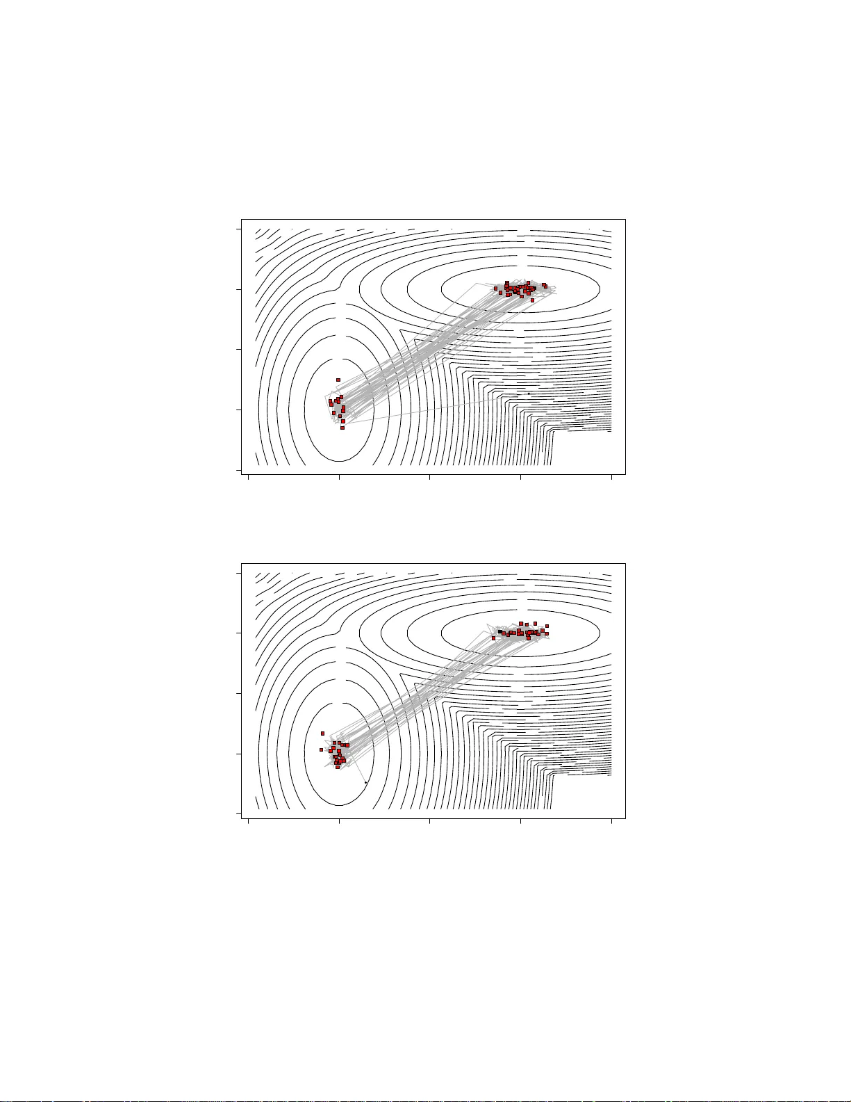
In teracting Multiple T ry Algorithms with Differen t Prop osal Distributio ns Rob erto Casarin †¶ Radu V. Craiu ‡ F abrizio Leisen § ¶ Adv anced School of Economics, V enice † Univ e r sit y of Brescia § Univ e r sidad Carlos II I de Madrid ‡ Univ e r sit y of T or on to Marc h 21, 2022 Abstract W e prop ose a new class of in teracting Markov chain Mo n te Carlo (MCMC) algorithms desig ned for increasing the efficiency of a mo dified m ultiple-tr y Metropo lis (MTM) algorithm. The extension with res pect to the ex is t ing MCMC literature is tw ofold. The s ampler prop osed ex- tends the basic MTM algorithm by allo wing differen t prop osal distri- butions in the mult iple- t r y generation step. W e exploit the structur e of the MTM algo r ithm with differe nt prop osal distributions to natura lly int r oduce an int er acting MTM mechanism (IMTM) that expands the class of p opulation Mon te Ca rlo metho ds. W e show the v alidit y o f the algorithm a nd discuss the choice o f the selectio n weigh ts a nd of the different prop osals. W e provide numerical studies which show that the new algo rithm can p erform better than the ba sic MTM algorithm and that the in tera c tio n mechanism a llo ws the IMTM to efficien tly explor e the state space. 1 In tro duction Mark o v c hain Mon te Carlo (MCMC) algorithms are no w essen tial for the analysis of complex statistical mo dels. In the MC MC univ ers e , one of the most widely used class of algorithms is defi n ed b y the Metrop olis-H astings (MH) (Metrop oli s et al., 1953; Hastings, 1970) and its v arian ts. An imp or- tan t generaliza tion of the standard MH form ulation is rep rese nted by the 1 m ultiple-try Metrop o lis (MTM) (Liu et al., 200 0 ). While in the MH form u- lation one accepts or rejects a single prop osed mo v e, the MTM is designed so that th e next state of the c hain is select ed among multiple p roposals. The m ultiple-prop osal setup can b e used effectiv ely to explore the sample space of the target d istribution and sub sequen t d evelo p men ts made u se of this added flexibilit y . F or instance, Craiu and Lemieux (2007) prop ose to u se antit h e tic and quasi-Mon te Carlo samples to generate the prop osals an d to improv e the efficiency of the algorithm while P and o lfi et al. (2010 b ) and P andolfi et al. (2010 a ) apply the m ultiple-prop osal idea to a trans-dimensional setup and com bine Rev ersib l e J ump MCMC with MTM. This wo rk f u rther generalizes the MTM algorithm presente d in Liu et al. (2000) in t wo d i r e ctions. First, we sho w that th e original MTM transition k ernel can b e modifi ed to allo w for differen t pr o p osal d istributions in th e m ultiple-try generation step while preserving the ergo dicit y of the c h a in. The use of different prop osal d i str i b utio n s giv es more freedom in d e signin g MTM algorithms f o r target distrib utio n s that require d iffe r e nt prop osals across the sample space. An imp ortan t c h a llenge remains the choic e of the distributions used to generate the prop osals and we prop ose to add ress it b y expanding up on methods u sed within the p opulation Mon te C a r l o class of algo r it h ms. The class of p opulation Monte Carlo pro cedures (Capp ´ e et al. , 2004 ; Del Moral a n d Miclo, 2000; Del Moral, 2004; J a sr a et al., 2007 ) h a s b een designed to address the inefficiency of classical MCMC samp le r s in complex applications inv olving multimod al and high dimensional target distributions (Pritc hard et al., 2000; Heard et al ., 2006 ) . Its formulatio n relies on a n um- b er of MCMC pro cesses that are run in parallel wh i le learning from one another ab out the geograph y of the target distrib utio n . A second contribution of the pap er is fi nding reliable generic metho ds for constructing the p roposal distribu ti ons for the MTM algorithm.W e pr o p ose an in teracting MCMC samp l in g design f o r the MTM that preserves the Mark o vian prop ert y . More sp eci fi c ally , in the prop osed interac ting MTM (IMTM) algorithm, we allo w the distinct prop osal distrib utio n s to use in- formation pro duced b y a p opulation of auxiliary c hains. W e infer th at the resulting p erformance of the MTM is tigh tly connected to the p erformance of the chai n s’ p opulation. In order to maximize the latter, w e prop ose a n u mb er of strategies that can b e used to tun e the auxiliary c hains. W e also adapt p revio u s extensions of the MTM and link the use of s to c hastic o v err e laxation, r a n dom-ra y Mon te Carlo metho d (see Liu et al., 2000) and sim ulated annealing to IMTM. In the next s ection we discuss the IMTM algorithm, pr o p ose a num b er 2 of alternativ e implement ations and prov e their ergo dicit y . In Section 3 we fo cus on some sp ecial cases of the IMTM alg orithm and in Section 4 the p erformance of the metho ds prop osed is d emo n strat ed with sim ulations and real examp les. W e end the pap er with a d iscu ssio n of f u ture directions for researc h. 2 In teracting Mon te Carlo Chains for MTM W e b egin by describing the MTM and it s extension for using differen t pro- p osal d i s tr i b utio n s. 2.1 Multiple-T r y Metropolis With Differen t Prop osal Dis- tributions Supp ose that of inte r e st is sampling from a distribution π that has su pp ort in Y ⊂ R d and is kn o wn up to a n o r ma lizing constan t. Assu ming that the current state of the c hain is x , the up date d e fi ned by the MTM algorithm of Liu et al. (2000) is d escrib ed in Algo rith m 1. Algorithm 1. Multiple-try M etr op olis Algorithm (MTM) 1. Dr aw M trial pr op osals y 1 , . . . , y M fr om the pr op osa l distribu- tion T ( ·| x ) . Compute w ( y j , x ) for e ach j ∈ { 1 , . . . , M } , wh er e w ( y , x ) = π ( y ) T ( x | y ) λ ( y, x ) , and λ ( y , x ) is a symmetric func- tion of x, y . 2. Sele ct y among the M pr op osals with pr ob ability pr op ortional to w ( y j , x ) , j = 1 , . . . , M . 3. Dr aw x ∗ 1 , . . . , x ∗ M − 1 variates fr om the distribution T ( ·| y ) and let x ∗ M = x . 4. A c c ept y with gener alize d ac c eptanc e pr ob ability ρ = min  1 , w ( y 1 , x ) + . . . + w ( y M , x ) w ( x ∗ 1 , y ) + . . . + w ( x ∗ M , y )  . Note that while th e MTM uses the same distr ib utio n to generate all the prop osals, it is possib l e to extend this formulation to different prop osal distributions without alte r in g the ergo dicit y of the asso ciated Mark o v c hain. 3 Let T j ( x, · ), w it h j = 1 , . . . , M , b e a set of prop osal d i s tr i b utio n s for whic h T j ( x, y ) > 0 if and only if T j ( y , x ) > 0. Define w j ( x, y ) = π ( x ) T j ( x, y ) λ j ( x, y ) j = 1 , . . . , M where λ j ( x, y ) is a nonn egativ e symm e tric function in x and y that can b e c hosen by the user. The only requirement is that λ j ( x, y ) > 0 whenev er T ( x, y ) > 0. T hen the MTM algo rith m with d iffe r e nt p roposal distributions is giv en in Algo rith m 2 . Algorithm 2. MTM with Differ ent Pr op osal Distributions 1. Dr aw indep e n dently M pr op osals y 1 , . . . , y M such that y j ∼ T j ( x, · ) . Compute w j ( y j , x ) for j = 1 , . . . , M . 2. Sele ct Y = y among the trial set { y 1 , . . . , y M } with pr ob ability pr op ortional to w j ( y j , x ) , j = 1 , . . . , M . L et J b e the index of the sele cte d pr op osa l. Then dr aw x ∗ j ∼ T j ( y , · ) , j 6 = J , j = 1 , . . . , M and let x ∗ J = x . 3. A c c ept y with pr ob ability ρ = min  1 , w 1 ( y 1 , x ) + · · · + w M ( y M , x ) w 1 ( x ∗ 1 , y ) + · · · + w M ( x ∗ M , y )  and r eje ct with pr ob ability 1 − ρ . It sh o u ld b e noted that Algorithm 2 is a sp ecial case of the interact in g MTM present ed in the next section and that the pro of of ergo dicit y for the asso ciate d chain follo ws closely the pr oof given in App endix A for the in teracting MTM and is n o t giv en here. In Section 4 w e will show, through sim ulation exp erimen ts, that this algorithm is more efficie nt then a MTM a lgorithm with a single prop osa l distribution. 2.2 General Construction Undoubtedly , Algorithm 2 offers additional flexibilit y in organizing the MT M sampler. This sectio n in tr o duces generic method s for using a p o p ulat ion of MCMC c hains to define th e pr o p osal distributions. 4 Algorithm 3. Inter acting Multiple T ry Algorithm (IMTM) • F or i = 1 , . . . , N 1. L et x = x ( i ) n , for j = 1 , . . . , M i dr aw y j ∼ T ( i ) j ( ·| x (1: i − 1) n , x, x ( i +1: N ) n ) indep endently and c omp u t e w ( i ) j ( y j , x ) = π ( y j ) T ( i ) j ( y j | x (1: i − 1) n , x, x ( i +1: N ) n ) λ ( i ) j ( y j , x ) . 2. Sele ct J ∈ { 1 , . . . , M i } with pr ob ability pr op ortional to w ( i ) j ( y j , x ) , j = 1 , . . . , M i and set y = y J . 3. F or j = 1 , . . . , M i and j 6 = J dr aw x ∗ j ∼ T ( i ) j ( ·| x (1: i − 1) n , y , x ( i +1: N ) n ) , let x ∗ J = x ( i ) n and c ompute w ( i ) j ( x ∗ j , y ) = π ( x ∗ j ) T ( i ) j ( x ∗ j | x (1: i − 1) n , y , x ( i +1: N ) n ) λ ( i ) j ( x ∗ j , y ) . 4. Set x ( i ) n +1 = y with pr ob ability ρ i = min ( 1 , w ( i ) 1 ( y 1 , x ) + . . . + w ( i ) M i ( y M i , x ) w ( i ) 1 ( x ∗ 1 , y ) + . . . + w ( i ) M i ( x ∗ M i , y ) ) and x ( i ) n +1 = x ( i ) n with pr ob ability 1 − ρ i . Consider a p opulation of N chains, X ( i ) = { x ( i ) n } n ∈ N and i = 1 , . . . , N . F or fu ll generalit y we assume that the i th c h a in has MTM transition k ernel with M i differen t prop osals { T ( i ) j } 1 ≤ j ≤ M i (if we set M i = 1 w e imply that the c hain h as a MH transition k ern e l). The inte r acting mechanism allo ws eac h prop osal d i str i b utio n to p o ssib l y dep e n d on th e v alues o f the c hains at the pr e vious step. F ormally , if Ξ n = { x ( i ) n } N i =1 is the v ector of v alues tak en at iteration n ∈ N b y the p opulation of c hains, then we allo w eac h p roposal distribution used in up dating the p opulation at iteration n + 1 to d e p end on Ξ n . The m a thematical formalization is used in th e description of Algorithm 3. One exp ects that the c hains in the p opulation are spr e ad thr o u gh ou t the sample sp ace and th us the prop osals generated are a go od represen tation of the samp l e space Y u lt imately resulting in b etter mixing f o r the c hain of 5 in terest. In order to give a r e p rese ntatio n of the IMTM transition d e n sit y let us in tro duce the follo wing notation. Let T ( i ) j ( x, y ) = T ( i ) j ( y | x (1: i − 1) n , x, x ( i +1: N ) n ), T ( i ) ( x, y 1: M i ) = Q M i k =1 T ( i ) k ( x, y k ) and T ( i ) − j ( x, y 1: M i ) = Q M i k 6 = j T ( i ) k ( x, y k ) and define dy 1: M i = Q M i k =1 dy k and dy − j = Q M i k 6 = j dy k . The transition densit y asso c iated to the p o p ulat ion of c hains is then K (Ξ n , Ξ n +1 ) = N Y i =1 K i ( x ( i ) n , x ( i ) n +1 ) (1) where K i ( x, y ) = M i X j =1 A ( i ) j ( x, y ) T ( i ) j ( x, y ) +   1 − M i X j =1 B ( i ) j ( x )   δ x ( y ) (2) is the tran s i tion ke r nel asso ciated to th e i -th c hain of algorithm with A ( i ) j ( x, y ) = Z Y 2( M i − 1) ˜ w ( i ) j ( y , x ) ρ ( i ) j ( x, y ) T ( i ) − j ( y , x ∗ 1: M i ) T ( i ) − j ( x, y 1: M i ) dx ∗ − j dy − j and B ( i ) j ( x ) = Z Y 2( M i − 1)+1 ρ ( i ) j ( x, y ) T ( i ) − j ( y , dx ∗ 1: M i ) T ( i ) ( x, dy 1: M i ) dx ∗ − j dy 1: M i . In the ab o v e equations ˜ w ( i ) j ( y j , x ) = w ( i ) j ( y j , x ) / ( w ( i ) j ( y , x ) + ¯ w ( i ) − k ( y 1: M i | x )), with j = 1 , . . . , M i and ¯ w ( i ) − j ( y 1: M i | x ) = P M i k 6 = j w ( i ) k ( y k , x ), are the normalized w eight s used in the selection step of th e IMTM algorithm and ρ ( i ) j ( x, y ) = min ( 1 , w ( i ) j ( y , x ) + ¯ w ( i ) − j ( y 1: M i | x ) w ( i ) j ( x, y ) + ¯ w ( i ) − j ( x ∗ 1: M i | y ) ) is the generalized MH ratio associated to a MTM a lgorithm. The v alidity of Algorithm 3 relies up on the detaile d b al ance condition. Theorem 1. The tr ansitio n density K i ( x ( i ) n , x ( i ) n +1 ) asso ciate d to the i -th chain of the IMTM algo rithm satisfies th e c onditional detaile d b alanc e d c on- dition. 6 Pro o f Se e App endix A. Since the transition K i ( x ( i ) n , x ( i ) n +1 ), i = 1 , . . . , N has π ( x ) as s t ationary distribution an d satisfies the conditional detailed b a lance condition th e n the join t transition K (Ξ n , Ξ n +1 ) has π ( x ) N as a sta tionary distrib utio n . An imp ortan t issue directly conn ected to the p rac tical implemen tation of the IMTM is th e c hoice of pr o p osal d istributions and the choice of λ ( i ) j ( x, y ). First it s h o u ld b e n o ted that at eac h iteration of the interact in g chains the compu t ational complexit y of th e algorithm is O ( N P N i =1 M i ). When considering the n umber of chains and the n umb er of prop osals, there are t wo possib le strategies in d e signin g the in teraction mec h a n i sm . The first strategy is to use a sm all num b er of c hains, say 2 ≤ N ≤ 5, in ord er to improv e the mixing of eac h c hain and to allo w for large jumps b et w een d i fferent regions of the state sp a ce. When applying this strategy to our IMTM algorithms it is p ossible to set the num b er of prop osals to b e equal to the n u m b er of c hains, i.e. M i = N , for a ll 1 ≤ i ≤ N . In this w ay all the chains can in teract at eac h iteration of the algorithm and many searc h directions can b e included among the p roposals. A second strateg y is to use a higher num b er of c h a in s, e.g. N = 100, in order to p ossibly hav e, at eac h iteration, a go od appro ximation of the target or a muc h higher n u mb er of searc h d i r e ctions for a go od exploration of the sample space. This algorithm design strategy is co mm o n in P opu la tion Mon te Carlo or Interact in g MCMC metho ds. Clearly when a h ig h num b er of chains is used within IMTM, it is necessary to set M i < N . In the next section w e discuss a f e w strategies to built the M i prop osals. 2.3 P arsing t he P opulation of Auxiliary Chains One of the strateg ies th a t reve aled to b e successful in our applicatio n s con- sists in the r a n dom selectio n of a certain num b er of c hains of the p opula- tion in order to build the prop osals. More sp ecifically , we let M i = M , for all i , and when up dating the i -th c hain of the p opulation w e sample I 1 , . . . , I M random in dexes from the u niform distr i b utio n U { 1 ,...,N } , with N > M , and then set the pr o p osals: T ( i ) j ( y , x ) = T ( i ) j ( ·| x, x ( I 1 ) n , . . . , x ( I M ) n ), for all j = 1 , . . . , M . On the basis of our sim u lation exp erimen ts we found that th e follo win g c hoice T ( i ) j ( · · · | x ( I 1 ) n , . . . , x ( I M ) n ) = T j ( ·| x ( I j ) n ) is works we ll in impro ving the mixing o f the c hains. Previously suggested f orm s for the fun c tion λ ( i ) j ( x, y ) (Liu et al., 2000) are: 7 a) λ ( i ) j ( x, y ) = 1 b) λ ( i ) j ( x, y ) = 2 { T ( i ) j ( x, y ) + T ( i ) j ( y , x ) } − 1 c) λ ( i ) j ( x, y ) = { T ( i ) j ( x, y ) T ( i ) j ( y , x ) } − α , α > 0. Here w e pr o p ose to include in the c hoice of λ the information pro vid ed by the p opulation of c hains. Therefore w e suggest to mo dify the ab o v e functions as follo ws a ′ ) λ ( i ) j ( x, y ) = ν j b ′ ) λ ( i ) j ( x, y ) = 2 ν j { T ( i ) j ( x, y ) + T ( i ) j ( y , x ) } − 1 c ′ ) λ ( i ) j ( x, y ) = ν j { T ( i ) j ( x, y ) T ( i ) j ( y , x ) } − α , α > 0 where the fac tor ν j captures the b eha viour of the auxiliary c h a in s at the previous iteratio n ν j = 1 N N X i =1 I { j } ( J ( i ) n − 1 ) , j = 1 , . . . , M where J ( i ) n − 1 is the random ind e x of the selection step at the iteration n − 1 for the i -th c hain. Th e mo difications prop osed for λ ( · , · ) wo u ld increase the use of those prop osal d i s tr i b utio n s fa v our e d by the pop u la tion of c hains a t pre- vious iteration. Since ν j dep ends only on s a mp le s generated at the p revio u s step by the p opulation of c hains, the ergo dicit y of the I M T M c hain is p re- serv ed. An alternativ e strategy is to samp le the random indexes I 1 , . . . , I M with probabilities prop ortio n al to ν j . 2.4 Annealed IMTM Our b e lief in IMTM’s impro ved p erformance is underpinn ed by the assump- tion that the p o p ula tion of Mon te Carlo c h a ins is spread throughout the sample space. T his can b e partly ac h i eved by initializing the c hains usin g dra ws f r o m a distrib utio n o verdisp ersed with resp ect to π (see also Jennison, 1993; Gelman and Rubin, 1992) and partly b y m o difying the stationary d is- tribution for s ome of the chains in the p o p ulat ion. Sp ecifically , we consider the sequ e n c e of annealed distribu t ions π t = π t with t ∈ { ξ 1 , ξ 2 , . . . , ξ N } , where 1 = ξ 1 > ξ 2 > . . . > ξ n , for instance ξ t = 1 /t . When t, s are close temp eratures, π t is similar to π s , b ut π = π 1 ma y b e m uc h h a r d er 8 to sample f rom than π ξ N as has b een long recognized in th e simulated an- nealing and sim ulated temp ering literature (see Marin ari and P arisi, 1992; Gey er and Thompson, 199 4 ; Neal, 1994 ) . Th e r e fore, it is lik ely that some of the c hains designed to sample from π 1 , . . . , π N ha ve go od mixing prop erties, making them go od candidates for th e p opulation of MCMC samp le r s needed for the IMTM. W e th us consider the Mont e Carlo p opulation made of the N − 1 c h a in s ha ving { π 2 , . . . , π N } as stationary distributions. An example of annealed in teracting MTM is giv en in Algo r i th m 4. Note that we let the i -th chain to in teract only with the N − i + 1 c h a in s at higher temperatur e by sampling I 1 , . . . , I M from U { 1 ,...,N − i +1 } . An astute reader ma y ha ve noticed that the use of MTM for e ach auxil- iary c hain ma y b e redund a nt since for smaller ξ i ’s the distrib u ti on π i is easy to sample fr o m. In Algorithm 5 we presen t an alternativ e implemen tation of the annealed IMTM in whic h eac h auxiliary c hain is MH with target π i , 1 ≤ i ≤ N − 1. Algorithm 4. Anne ale d IM TM A lgorithm (A IMTM1) • F or i = 1 , . . . , N 1. L et x = x ( i ) n and sample I 1 , . . . , I M fr om U { 1 ,...,N − i +1 } . 2. F or j = 1 , . . . , M dr aw y j ∼ T ( i ) j ( ·| x ( I j ) n ) indep endently and c ompute w ( i ) j ( y j , x ) = π ( y j ) T ( i ) j ( y j | x ( I j ) n ) λ ( i ) j ( y j , x ) . 3. Sele ct J ∈ { 1 , . . . , M } with pr ob ability pr op ortional to w ( i ) j ( y j , x ) , j = 1 , . . . , M and set y = y J . 4. F or j = 1 , . . . , M and j 6 = J dr aw x ∗ j ∼ T ( i ) j ( ·| x (1: i − 1) n , y , x ( i +1: N ) n ) , let x ∗ J = x ( i ) n and c ompute w ( i ) j ( x ∗ j , y ) = π ( x ∗ j ) T ( i ) j ( x ∗ j | y ) λ ( i ) j ( x ∗ j , y ) . 5. Set x ( i ) n +1 = y with pr ob ability ρ i , wher e ρ i is the gener alize d M.H. r atio of the IMT algorithm and x ( i ) n +1 = x ( i ) n with pr ob ability 1 − ρ i . 9 Algorithm 5. Anne ale d IM TM A lgorithm (A IMTM2) • F or i = 1 1. L et x = x ( i ) n and sample I 1 , . . . , I M fr om U { 1 ,...,N } . 2. F or j = 1 , . . . , M dr aw y j ∼ T ( i ) j ( ·| x ( I j ) n ) indep endently and c ompute w ( i ) j ( y j , x ) = π ( y j ) T ( i ) j ( y j | x ( I j ) n ) λ ( i ) j ( y j , x ) . 3. Sele ct J ∈ { 1 , . . . , M } with pr ob ability pr op ortional to w ( i ) j ( y j , x ) , j = 1 , . . . , M and set y = y J . 4. F or j = 1 , . . . , M and j 6 = J dr aw x ∗ j ∼ T ( i ) j ( ·| x (1: i − 1) n , y , x ( i +1: N ) n ) , let x ∗ J = x ( i ) n and c ompute w ( i ) j ( x ∗ j , y ) = π ( x ∗ j ) T ( i ) j ( x ∗ j | y ) λ ( i ) j ( x ∗ j , y ) . 5. Set x ( i ) n +1 = y with pr ob ability ρ i , wher e ρ i is the gener alize d M.H. r atio of the IMT algorithm and x ( i ) n +1 = x ( i ) n with pr ob ability 1 − ρ i . • F or i = 2 , . . . , N 1. L et x = x ( i ) n and up date the pr op osal f u nctio n T ( i ) ( ·| x ) . 2. Dr aw y ∼ T ( i ) ( ·| x ) and c ompute ρ i = min ( 1 , π ( y ) ξ i T ( i ) ( x | y ) π ( x ) ξ i T ( i ) ( y | x ) ) . 3. Set x ( i ) n +1 = y with pr ob ability ρ i and x ( i ) n +1 = x ( i ) n with pr ob- ability 1 − ρ i . The chain of int erest, corresp o n ding to ξ = 1, h a s an MT M transition k ernel w i th M = N − 1 p roposal distributions. A t time n the j th prop osal distribution used for the c hain ergodic to π is T (1) j = T ( j ) , is the same as the prop osal used b y the j th auxiliary c hain, for all 2 ≤ j ≤ N . 10 An add it ional gain could b e obtained if the auxiliary chains’ transition k ernels are mo dified using adaptive MCMC strategies (see also Chauve au and V andekerkho v e , 2002, for another example of adaption for int eracting c hains). Ho w eve r , it should b e noted that letting the auxiliary c hains adapt indefin it ely results in complex th e oretical justifications for the IMTM which go b ey ond the scop e of this pap er and will b e presen ted e lsewh ere. Ou r current recommendation is to use finite adaptation for the auxiliary chains prior to th e start of the IMTM. O ne could tak e adv an tage of multi-processor computing units and use parallel pr o grammin g to increase the computational efficiency of this approac h. The adap tation of λ ( i ) j ( · , · ), through the w eigh ts ν j defined in the previous section, should b e u sed cautiously in this case. Th e aim of th e annealing pro cedure is to allo w the higher temp eratures chains to explore widely the sample space and to improv e the mixing of th e MTM c hain. Using ν j the con text of ann e aled IMT M could arbitrarily p enalize some of the higher temp erature pr o p osals and reduce the effectiv eness of the annealing str a tegy . It is p ossible to hav e a Mont e Carlo appr o ximatio n of a quantit y of in terest by using the outpu t pro duced b y all the c h a ins in the p opulation. F or example let I = Z Y h ( x ) π ( x ) dx b e the qu antit y of interest where h is a test function. It is p ossible to appro ximate this quant ity as follo ws I N T = 1 T T X n =1 1 ¯ ζ N X j =1 h ( x ( j ) n ) ζ j ( x ( j ) n ) where x ( i ) n , with n = 1 , . . . , T and i = 1 , . . . , N is the output of a IMTM c hains with target π ξ i and ζ j ( x ) = π ( x ) /π ξ j ( x ) is a set of imp ortance w eights with normalizing constan t ¯ ζ = P N j =1 ζ j ( x ( j ) n ). 2.5 Gibbs within IMTM up date It sh o u l d b e noticed th at in the prop osed algorithm at the n -th iterat ion the N c hains are up dated sim u lt aneously . In the interact in g MCMC literature a sequen tial up dating sc heme (Gibbs-lik e u pd a ting) has b een pr o p osed for example in Mengersen and Ro b ert (2003) and Campillo et al. (2009). In the follo wing w e sho w that the Gibbs-lik e up dating also apply to our IMTM con text. In th e Gibbs-lik e inte r a cting MTM (GIMTM) algorithm giv en in 11 Algorithm 6 the d i fferent prop osa ls fu nctio n s of the i -th c hain, w i th i = 1 , . . . , N , ma y dep end on the current v alues of th e up date d chains x ( j ) n +1 , with j = 1 , . . . , ( i − 1) and on the last v alues x ( j ) n , with j = ( i + 1) , . . . , N , of the chains whic h ha v e n o t y et b een up date d . Algorithm 6. Gibbs-like IMTM Algorith m (GIMTM ) • F or i = 1 , . . . , N 1. F or j = 1 , . . . , M i dr aw y j ∼ T ( i ) j ( ·| x (1: i − 1) n +1 , x ( i ) n , x ( i +1: N ) n ) i n- dep e ndently and c ompute w ( i ) j ( y j , x ) = π ( y j ) T ( i ) j ( y j | x (1: i − 1) n +1 , x ( i ) n , x ( i +1: N ) n ) λ ( i ) j ( y j , x ( i ) n ) . 2. Sele ct J ∈ { 1 , . . . , M i } with p r ob ability pr op ortion al to w ( i ) j ( y j , x ) , j = 1 , . . . , M i and set y = y J . 3. F or j = 1 , . . . , M i and j 6 = J dr aw x ∗ j ∼ T ( i ) j ( ·| x (1: i − 1) n +1 , y , x ( i +1: N ) n ) , let x ∗ J = x ( i ) n and c ompute w ( i ) j ( x ∗ j , y ) = π ( x ∗ j ) T ( i ) j ( x ∗ j | x (1: i − 1) n +1 , y , x ( i +1: N ) n ) λ ( i ) j ( x ∗ j , y ) . 4. Set x ( i ) n +1 = y with pr ob ability ρ i = min ( 1 , w ( i ) 1 ( y 1 , x ) + . . . + w ( i ) M i ( y M i , x ) w ( i ) 1 ( x ∗ 1 , y ) + . . . + w ( i ) M i ( x ∗ M i , y ) ) and x ( i ) n +1 = x ( i ) n with pr ob ability 1 − ρ i . In the GIMTM algorithm th e iteration mec hanism b et w een the c hains is not the same as in the IMT M a lgorithm. The c hains are n o longer ind e p en- den t since the p r o p osals ma y dep end on the current v alues for some of the c hains in the p opulatio n . Th e transition k ernel for the whole p opulation is K (Ξ n , Ξ n +1 ) = N Y i =1 K i ( x ( i ) n , x ( i ) n +1 | x (1: i − 1) n +1 , x ( i +1: N ) n ) and in this case the v alidit y of the algorithm still relies u pon the conditional detail balance co n ditio n give n f o r the IMTM algorithm. 12 Finally w e remark that th e GIMTM algorithm allo ws us to introdu c e further p ossible c hoices f o r the λ ( i ) j ( x, y ) functions. In particular a repu lsiv e factor (see Mengersen and Robert (2003)) can b e introd uce d in the selection w eight s in order to indu c e negativ e dep endence betw een the chains. W e let the study of the GIMTM algorithm and the use of repulsive factors for futur e researc h and fo cus instead on the p roperties of the IMTM algorithm. 3 Some generalizations In the f o llo w i n g we will discuss some p ossible generalizati on of the IMTM algorithm. Firs t w e sho w how to use the sto c hastic o verrela xation metho d to p ossibly h a v e a further gain in the efficiency . Secondly w e sugge s t t w o p ossible str ategies to built the differen t prop osal fu n ct ions of the IMTM. The first strategy consists in prop osing v alues along different searc h direc- tions and represen ts an extension of the random-ra y Mont e Carlo algorithm present ed in Liu et al. (2000). T he second strategy relies up on a suitable com bination of target temperin g and adaptiv e MCMC c hains. 3.1 Sto c hastic Ov errelaxation Sto c hastic o v err e laxation (SOR) is a Mark ov c hain Mont e Carlo tec h n ique dev elop ed by Adler (1981) for normal d e n sit ies and s ubsequen tly extended b y Green and Han (1992 ) for non-normal targets. The idea b ehind this approac h is to induce n e gativ e correlati on b e tw een consecutiv e dr a ws of a single MCMC pro c ess. Within the MTM algorithm w e can implement SOR by indu c in g negativ e correlation b et w een the prop osals and b et wee n the prop osals and the cur ren t state of the c hain, x . A n a tu r a l an d easy to implemen t p rocedure ma y b e based on the assumption that ( y 1 , . . . , y M − 1 , x ) T ∼ N d × M ( 0 , V ) where V ’s structure is dictat ed by th e desired n eg ativ e dep endence b et w een the prop osals y 1 , . . . , y n ’s and x , sp ecifically V =     Σ 1 Ψ 12 . . . Ψ 1 M Ψ 12 Σ 2 . . . Ψ 2 M . . . . . . . . . . . . Ψ 1 M Ψ 2 M . . . Σ M     . F or instance, w e can set Ψ ij = 0 w henev er i, j 6 = M and Ψ iM = Σ 1 / 2 i R iM Σ 1 / 2 M where R iM is a correlation matrix whic h corresp onds to ex- treme negativ e correlation (see Cr a iu and Meng, 200 5 , for a discus sio n of 13 extreme dep endence) b et we en any t wo comp o n ents (with same index) of y i and x , for an y 1 ≤ i ≤ M − 1. The general construction falls within the con text of d e p endent pr o p osals as discussed by Craiu and Lemieux (2007) with the additional b onus of ”pulling” the prop osals a wa y f rom the cur- ren t state due to the imp osed n egativ e correlation. This essen tially ensur e s that n o prop osals are exceedingly close to the cu rren t lo catio n of the c hain. Also note that the constru ction is general enough a n d can b e applied for Algorithms 2 and 3 as long as the prop osal distribu ti ons are Gaussian. 3.2 Multiple Random-ra y Mon te Carlo W e show h e r e that the u se of different prop osals for the MTM alg orithm allo ws also to extend the random-ra y Monte Carlo metho d give n in Liu et al. (2000). In particular the p roposed algorithm allo ws to deal with multiple searc h dir e ctions at eac h iteration of th e c hains. At the n -th iteration of the c hain, in order to up date the set of chains Ξ n , the algorithm p erforms for eac h c h a in x ( r ) n ∈ Ξ n , with r = 1 , . . . , N , the follo wing steps: 1. Ev aluate the gradien t log π ( x ) at x ( r ) n and find th e mo de a n along x ( r ) n + r u n where u n = x ( r ) n − x ( r ) n − 1 . 2. Samp le I 1 , . . . , I M from the uniform U { 1 ,...,r − 1 ,r +1 ,...,N } . 3. Let e n,j = ( a n − x ( I j ) n ) / || a n − x ( I j ) n || and sample r j from N (0 , σ 2 ). and then use the set of prop osa ls T j whic h dep ends on e n,j to p erform a MTM trans ition with different prop osals as in the IMTM algorithm (see Alg. 1). 4 Sim ulation Results 4.1 Single-c hain r esults In this section we carr y out, through some examples, a comparison b et wee n the single-c hain multiple try algorithms MT M-DP with differen t p roposals and the algorithm in Liu et al. (2000 ). In the MTM-DP algorithm we consider four Gaussian random-wal k prop osal s y j ∼ N n ( x , Λ j ) w i th Λ 1 = 0 . 1 I d n , Λ 2 = 5 I d n , Λ 3 = 50 I d n and Λ 4 = 100 I d n , wh e r e I d n denotes th e n -order identit y matrix. In the MTM sele ction w eight s w e set λ j ( x , y ) = 2 α j / ( T j ( x , y ) + T j ( y , x )), where α j = 0 . 25, for j = 1 , . . . , 4. 14 In order to compare the MTM algorithm with different prop osals and the Multiple T r y algorithm of Liu et al. (2000) we consider 20,000 iterations and use f o u r trials y j generated b y the follo wing prop osal T j ( x , y j ) = 4 X j =1 α j N n ( x , Λ j ) (3) where Λ j , j = 1 , . . . , 4, hav e b een defined ab o v e. In the weig h s of the selection step w e set λ ( x , y ) = 2 / ( T j ( x , y ) + T j ( y , x )). 4.1.1 Biv a riate Mixture with tw o comp onen t s W e consider the follo wing biv ariate mixture of t wo normals 1 3 N 2 ( µ 1 , Σ 1 ) + 2 3 N 2 ( µ 2 , Σ 2 ) (4) with µ 1 = (0 , 0) ′ , µ 2 = (10 , 10) ′ , Σ 1 = diag(0 . 1 , 0 . 5) and Σ 2 = diag(0 . 5 , 0 . 1). In Fig. 1 the A CF with 30 lags for the first comp onent of the biv ari- ate MH c h ain. Th e au to correlation is lo wer for the MTM a lgorithm with differen t prop osals. 4.1.2 Multiv ariate Normal Mixture W e compare the algorithms for high-d im en sional targets. W e consider the follo wing m u ltiv ariate mixtu re of tw o normals with a sparse v ariance-co v ariance structure 1 3 N 20 ( µ 1 , Σ 1 ) + 2 3 N 20 ( µ 2 , Σ 2 ) (5) with µ 1 = (3 , . . . , 3) ′ , µ 2 = (10 , . . . , 10) ′ and Σ j , with j = 1 , 2, generate d indep en d en tly from a Wishart distribution Σ j ∼ W 20 ( ν, I d 20 ) wh ere ν is the degrees of f reedom parameter of the Wishart. In the exp erimen ts w e set ν = 21. The auto correlation function of the chain for one of the experiment is giv en in Fig. 2. The ACF has b een ev aluated for eac h comp onen ts of the 20-dimensional c hain. The v alues of the ACF of the MTM-DP (blac k lines in Fig. 2) are less than th ose of the original MTM (gra y lines of the same figure) in all the dir ections of the su p p ort space. W e conclude that the MTM algorithm with differen t prop osals (Algorithm 3) outp erforms the Liu et al. (2000) MTM alg orithm. 15 0 5 10 15 20 25 30 0.88 0.90 0.92 0.94 0.96 0.98 1.00 MTM MTM−DP Figure 1: Auto correlation f unction of the Liu’s MTM (gra y line) a n d MTM with differen t prop osals (blac k line). 0 5 10 15 20 25 30 0.90 0.92 0.94 0.96 0.98 1.00 MTM MTM−DP Figure 2: Autocorrelation fun ction (A CF) of the 20 comp onen ts of the m u l- tiv ariat e MH c hain for the Liu’s MT M (g r ay lines) and MTM with different prop osals (blac k lines). 16 4.2 Multiple-c hains results In this section we show real and sim ulated data results of the g en er al in ter- acting m ultiple try algo rith m in Alg. 1. 4.2.1 Biv a riate Mixture with tw o comp onen t s The target distribution is the follo wing biv ariate mixture of t wo normals 1 3 N 2 ( µ 1 , Σ 1 ) + 2 3 N 2 ( µ 2 , Σ 2 ) (6) with µ 1 = (0 , 0) ′ , µ 2 = (10 , 10) ′ , Σ 1 = diag(0 . 1 , 0 . 5) and Σ 2 = diag(0 . 5 , 0 . 1). W e consider a p op u lation of N = 50 c hains with M = 50 prop osals and 1,000 iterations of the IMTM algorithm. F or eac h c hain we consid er the case T ( i ) j ( y | x (1: i − 1) n +1 , x ( i ) n , x ( i +1: N ) n ) = T ( j ) ( y , x ( j ) n ) and dr a w y j ∼ N 2 ( x ( j ) n , Λ j ) (7) where Λ j = (0 . 1 + 5 j ) I d 2 . In this sp ecification of the IMTM algorithm eac h c hain has M ind ep endent p rop osals with co n ditional mean giv en by the previous v alues of the c hains in the p opulation. In this exp eriment we consider tw o kind of weig hts. First we set λ ( i ) j ( x, y ) = ( T ( i ) j ( x, y ) T ( i ) j ( y , x )) − 1 , that corresp ond s to use imp ortance sampling selec- tion weig hts, secondly w e consider λ ( i ) j ( x, y ) = 2( T ( i ) j ( x, y ) + T ( i ) j ( y , x )) − 1 , whic h implies a symmetric MTM algorithm. W e denote with I MT M-IS and IMTM-T A resp ectiv ely the resulting algo r ithms. Fig. 3 sho w the r esults of the IMTM-IS and IMTM-T A al gorithms at the last iteration o f the p opulation of c h ains (bla ck dots). In b oth of the algorithms the p opulation is visiti n g the tw o mo des of the d istr ibution in the right p rop ortion. Moreo v er eac h c hain is able to j ump from one mo d e to the other. (the light- gray line repr esen ts the sample path of one of the c hain). 4.2.2 Beta-Binomial Mo del W e consider here the pr oblem of the genetic instabilit y of esophageal can- cers. During a neoplastic pr ogression the cancer cells un dergo a num b er of genetic changes and p ossibly lose entire c hr omosome sections. Th e loss of a c hromosome section con taining one allel e b y abnormal cell s is cal led L oss of Heter ozygosity (LOH). The L OH can b e detected us in g lab oratory assa ys 17 −700 −680 −660 −640 −620 −600 −580 −560 −540 −520 −500 −480 −460 −440 −420 −400 −380 −360 −340 −320 −300 −280 −280 −260 −260 −240 −240 −220 −220 −200 −200 −180 −180 −160 −160 −140 −140 −140 −120 −120 −100 −100 −80 −80 −60 −60 −40 −40 −20 −20 −5 0 5 10 15 −5 0 5 10 15 −700 −680 −660 −640 −620 −600 −580 −560 −540 −520 −500 −480 −460 −440 −420 −400 −380 −360 −340 −320 −300 −280 −280 −260 −260 −240 −240 −220 −220 −200 −200 −180 −180 −160 −160 −140 −140 −140 −120 −120 −100 −100 −80 −80 −60 −60 −40 −40 −20 −20 −5 0 5 10 15 −5 0 5 10 15 Figure 3: Log-ta r get lev el sets (solid lines), the MH chains (red dots) at the last iteration of the IMTM algorithms and th e p ath of one of the chain of the set (gra y line). Up: output of the IMTM-IS with imp ortance sampling selection w eight s. Bottom: ouput of the IMTM-T A with symmetric lam b da as in (c). 18 on patients with tw o different allele s for a particular gene. Chromosome re- gions con taining genes whic h r egulate cell b ehavi or, are hyp othesized to ha ve a high rates of LOH. Consequen tly the loss of these c h romosome sections disables imp ortant cellular con trols. Chromosome regions with h igh rates of LOH are hyp othesized to conta in T umor Suppr essor Genes (TSGs), whose d eactiv ation contributes to th e dev elopment of esophageal cancer. Moreo ver the neoplasti c progression is though t to pro d uce a high level of b ac kground LOH in all c hromosome regions. In ord er to discriminate b etw een ”bac kground ” and TS Gs LO H, the Seattle Barrett’s Esophagus researc h pro j ect (Barrett et al. (1996)) has col- lected LOH rates from esophageal ca n cers for 40 regions, eac h on a distinct c hromosome arm. The lab eling of the t wo groups is unkn o wn so Desai (2000) suggest to consider a m ixture m o del for the frequency of LOH in b oth the ”bac kground” and TSG groups. W e consider the hierarc hical Beta-Binomial m ixtu re mo del p rop osed in W arnes (2001) f ( x, n | η , π 1 , π 2 , γ ) = η  n x  π x 1 (1 − π 1 ) n − x + (8) (1 − η )  n x  Γ(1 /ω 2 ) Γ( π 2 /ω 2 )Γ((1 − π 2 ) /ω 2 ) Γ( x + π 2 /ω 2 )Γ( n − x + (1 − π 2 ) /ω 2 ) Γ( n + 1 /ω 2 ) with x num b er of LOH sections, n th e num b er of examined sections, ω 2 = exp { γ } / (2(1 + exp { γ } )). Let x = ( x 1 , . . . , x m ) and n = ( n 1 , . . . , n m ) b e a set of observ ations from f ( x, n | η , π 1 , π 2 , γ ) and let us assume the follo wing priors η ∼ U [0 , 1] , π 1 ∼ U [0 , 1] , π 2 ∼ U [0 , 1] and γ ∼ U [ − 30 , 30] (9) with U the uniform distribution on [ a, b ]. Then the p osterior distribu tion is π ( η , π 1 , π 2 , γ | x , n ) ∝ m Y j =1 f ( x j , n j | η , π 1 , π 2 , γ ) (10) The p arametric sp ace is of dimension four: ( η, π 1 , π 2 , γ ) ∈ [0 , 1] 3 × [ − 30 , 30] and the p osterior distribution has t wo we ll-separated mo des making it d if- ficult to sample usin g generic m etho ds. W e apply the I MTM algorithm with 100 iterations, M = 4 p rop osal functions rand omly selected b et we en a p opu lation of N = 100 chains. F or eac h c h ain w e consider imp ortance sampling w eights in the selection step, 19 0.0 0.2 0.4 0.6 0.8 1.0 0.0 0.2 0.4 0.6 0.8 1.0 π 1 π 2 Figure 4: V alues of the p opulation of c hains (dots) at the last iteration on the sub space ( π 1 , π 2 ). The in teraction is giv en by M = 4 prop osal functions randomly selecte d b etw een the p op u lation of N = 100 c hains. i.e. we set λ ( i ) j ( x, y ) = ( T ( i ) j ( x, y ) T ( i ) j ( y , x )) − 1 with j = 1 , . . . , 4 and i = 1 , . . . , 100. The v alues of the p opulation of chains (dots) at the last iteration on the sub space ( π 1 , π 2 ) is giv en in Fig. 4.2.2. The IMTM is able to visit b oth r egions of the parameter sp ace confirmin g the analysis of Craiu et al. (2009) and W arn es (2001). 4.2.3 Stochastic V olatility The estimation of the sto c hastic v olatilit y (SV) mo del due to T aylo r (1994) still represen ts a c hallenging issue in b oth off-li n e (Celeux et al. (2006)) and sequen tial (Casarin and Marin (2009)) inference co ntexts. One of the main difficulties is due to the high dimension of the sampling space wh ich hind ers the u se of the data-augmen tation and prev en ts a r eliable join t estima tion of the parameters and the laten t v ariables. As highligh ted in Casarin et al. (2009) u sing multiple c hains with a chai n inte r action mechanism could lead to a substan tial impro v ement in the MCMC metho d for this kin d of mo del. 20 W e consider the SV mod el given in Celeux et al. (2 006 ) y t | h t ∼ N  0 , e h t  h t | h t − 1 , θ ∼ N  α + φh t − 1 , σ 2  h 0 | θ ∼ N  0 , σ 2 / (1 − φ 2 )  with t = 1 , . . . , T an d θ = ( α , φ , σ 2 ). F or the parameters we assume the noninformativ e prior (see Celeux et al., 2006) π ( θ ) ∝ 1 / ( σ β ) I ( − 1 , 1) ( φ ) where β 2 = exp( α ). In order to sim ulate from the p osterior w e consider the full co n ditional distributions and apply a Gibbs alg orithm . If w e define y = ( y 1 , . . . , y T ) and h = ( h 0 , . . . , h T ) then th e full cond itionals for β and φ are the in v erse gamma distributions β 2 | h , y ∼ I G T X t =1 y 2 t exp( − h t ) / 2 , ( T − 1) / 2 ! σ 2 | φ, h , y ∼ I G T X t =2 ( h t − φh t − 1 ) 2 / 2 + h 2 1 (1 − φ 2 ) , ( T − 1) / 2 ! and φ and the laten t v ariables ha v e n on-standard full conditionals π ( φ | σ 2 , h , y ) ∝ (1 − φ 2 ) 1 / 2 exp − φ 2 2 σ 2 T − 1 X t =2 h 2 t − φ σ 2 T X t =2 h t h t − 1 ! I ( − 1 , +1) ( φ ) π ( h t | α, φ, σ 2 , h , y ) ∝ exp  − 1 2 σ 2  ( h t − α − φh t − 1 ) 2 − ( h t +1 − α − φh t ) 2  − 1 2  h t + y 2 t exp( − h t )   . In order to sample f r om the p osterior we use an IMTM within Gibbs algo- rithm. A d etailed descrip tion of the prop osal distr ib utions for φ and h t can b e found in Celeux et al. (20 06 ). W e consider the t w o parameter settings ( α , φ , σ 2 ) = (0 , 0 . 99 , 0 . 01) and ( α , φ , σ 2 ) = (0 , 0 . 9 , 0 . 1) which corresp ond, in a fi n ancial s to c k m ark et con- text, to daily and w eekly frequency data resp ectiv ely . Note that as rep orted in Casarin and Marin (2009) inference in the daily example is more d ifficult. W e co m p are the p erformance of MH within Gibbs and IMTM within Gibb s algorithms in te r ms of Mean Square Err or (MSE) for the parameters and 21 of cum ulativ e RMSE for the lat ent v ariables. W e carry out the compari- son in statistical terms and estimate the MSE and RMS E b y ru nning the algorithms on 20 indep endent sim u lated datasets of 200 observ ations. In the comparison we tak e in to account the computational cost and for the IMTM within Gibbs w e use N = 20 inte r acting c hains, 1,00 0 iterations and M = 5 p rop osal f u nctions. Th is setting corresp onds to 100,00 0 ran d om dra ws and is equ iv alen t to the 100,0 00 iterations of the MH within Gibbs algorithm used in the comparison. Note that th e p rop osal step of the IMTM selects at random the p rop osal fu n ctions b etw een the other c hains and the selection step u ses λ ( i ) j ( x, y ) = ( T ( i ) j ( x, y ) T ( i ) j ( y , x )) − 1 , with h = 1 , . . . , 5 and i = 1 , . . . , 20. The r esults for the parameter estimation when applying IMTM are pre- sen ted in T able 1 and sho w an effectiv e impro v ement in the estimat es, b oth for we ekly and daily data, when compared to the results of a MH algorithm with an equiv alent computational load. Daily Da ta W eekly Data θ V alue MSE θ V alue MSE IMTM MH IMTM MH α 0 0.04698 0.0951 7 α 0 0.00146 0.00849 (0.006 12) (0.0019 4) (0.001 39) (0.0010 5) φ 0.99 0.20109 0.34825 φ 0.9 0.0132 8 0.107 46 (0.024 14) (0.0518 7) (0.040 14) (0.0362 9) σ 2 0.01 0.00718 0.0238 0 σ 2 0.1 0.0013 6 0.091 75 (0.001 73) (0.0020 2) (0.001 41) (0.0035 8) T able 1: Mean square error (MSE ) and its standard d eviation (in paren- thesis) for the parameter estimation with IMTM and MH within Gibbs algorithms. Left panel: daily datasets. Righ t panel: weekly dataset . A t ypical outpu t of the IMTM for some c hains of the popu lation and for the laten t v ariables h is giv en in Fig. 4.2.3. Eac h chart sho ws for a giv en c h ain the estimated latent v ariables (dotted blac k line), the p osterior quan tiles (gra y lines) and the true v alue of h (solid blac k line). Figures 4.2.3 and 4.2.3 exhibit the HPD regio n at the 90% (gra y areas) and the m ean (blac k lines) of the cumulativ e RMS E of eac h algorithm for the w eekly and daily data, resp ectiv ely . The statisti cs hav e b een estimate d from 20 indep endent exp eriments. The a ve r age RMSE sho ws that, in b oth parameter settings consid ered h ere, the IMTM (dashed blac k line) is more 22 efficien t than the standard MH algorithm (solid blac k line). 5 Conclusions In this pap er we prop ose a new class of interacting Metrop olis alg orithm, with Mu ltiple T ry transition. These algorithms extend the existing literature in tw o directions. First we show a natural and n ot straightforw ard wa y to include the c hains inte r action in a multiple try transition. Secondly the m ultiple try transitio n has been extended in order to acco u n t for the use of differen t prop osal fu nctions. W e giv e a pro of of v alidit y of the algorithm and show on real and sim u lated examples the effectiv e impro vemen t in th e mixing prop erty and exploratio n abilit y of the resulting in teracting c hains. App endix A Pro of Without loss of gener ality, we dr op the chain index i and the iter ation i ndex n , set M i = N , ∀ i and x ( i ) n = x and denote with T j ( y , x ) = T j ( y | x (1: i − 1) n +1 , x ( i ) n , x ( i +1: N ) n ) λ ( i ) j ( y j , x ( i ) n ) th e j pr op osal of the i -th chain at the iter ation n c onditional on the p ast and curr ent val u es, x (1: i − 1) n +1 and x ( i +1: N ) n r esp e ctively, of th e other chains. L et us define the fol lowing quantities ¯ w ( y 1: N | x ) = N X j =1 w j ( y j , x ) , ¯ w − k ( y 1: N | x ) = N X j 6 = k w j ( y j , x ) and S N ( J ) = 1 ¯ w ( y 1: N | x ) N X j =1 δ j ( J ) w j ( y j , x ) with J ∈ J = { 1 , . . . , N } the empiric al me asur e g e ner ate d by differ ent pr o- p osa ls and by the normalize d sele ction weights. L et T ( x, dy 1: N ) = N N j =1 T j ( x, dy j ) : ( Y × B ( Y N )) 7→ [0 , 1] the j oint pr o- p osa l for the multiple try and define T − k ( x, dy 1: N ) = N N j 6 = k T j ( x, dy j ) . L et A ( x, y ) b e the actual tr ansition pr ob ability for moving fr om x to y in the IMT2 algor ithm. Sup p ose that x 6 = y , then the tr ansition is a r esults two steps. Th e first step is a sele ction step which c an b e written as y = y J 23 0 50 100 150 200 −3 −1 1 2 3 0 50 100 150 200 −3 −1 1 2 3 0 50 100 150 200 −3 −1 1 2 3 0 50 100 150 200 −3 −1 1 2 3 0 50 100 150 200 −3 −1 1 2 3 0 50 100 150 200 −3 −1 1 2 3 0 50 100 150 200 −3 −1 1 2 3 0 50 100 150 200 −3 −1 1 2 3 Figure 5: T yp ical output of the p opu lation of chains for a weekly dataset. F or ea ch c hain the estimated laten t v ariable (dotted black line), th e 2.5% and 97.5 % quant iles (gra y lines) and the true v alue of h (solid blac k line). 24 0 50 100 150 200 0.0 0.2 0.4 0.6 0.8 0 50 100 150 200 0.0 0.5 1.0 1.5 Figure 6: Cumulat ive RMSE for the IMTM (dashed line) and MH (solid line) and the 90% HPD r egions for the IMTM (ligh t gray) and MH (dark gra y) estimate d on 20 indep end en t exp er im ents for b oth the d aily (up) and w eekly (b ottom) data sets. 25 and x ∗ J = x with the r andom i ndex J sample d fr om th e empiric al me asur e S N ( J ) . The se c ond step is a ac c ept/r eje ct step b ase d on the gener alize d MH r atio which involves the gener ation of the auxiliary values x ∗ j for j 6 = J . Then π ( x ) A ( x, y ) = = π ( x ) Z Y N T ( x, dy 1: N ) Z J S N ( dJ ) Z Y N − 1 ×Y 2 T − J ( y , dx ∗ 1: N ) × × δ x ( dx ∗ J ) δ y J ( dy ) min  1 , ¯ w ( y 1: N | x ) ¯ w ( x ∗ 1: N | y )  = π ( x ) N X j =1 Z Y N − 1 T − j ( x, dy 1: N ) T j ( x, y ) Z Y N − 1 T − j ( y , dx ∗ 1: N ) × × w j ( y , x ) w j ( y , x ) + ¯ w − j ( y 1: N | x ) min  1 , w j ( y , x ) + ¯ w − j ( y 1: N | x ) w j ( x, y ) + ¯ w − j ( x ∗ 1: N | y )  = N X j =1 w j ( x, y ) w j ( y , x ) λ j ( y , x ) Z Y 2( N − 1) T − j ( x, dy 1: N ) × × T − j ( y , dx ∗ 1: N ) min  1 w j ( y , x ) + ¯ w − j ( y 1: N | x ) , 1 w j ( x, y ) + ¯ w − j ( x ∗ 1: N | y )  which is symmetric in x and y. References Barrett, M. , Gal ipeau, P. , Sanchez, C. , Emond , M . and Reid, B. (1996). Determination of the fr equency of loss of heterozygosit y in esophageal adeno-carcinoma nu cell sorting, whole genome amplification and microsatel lite p olymorph isms. Onc o gene 12 . Campillo, F. , Rakotozafy, R. and Rossi, V. (2009). Paral lel and inter- acting Mark ov c hain Mon te Carlo algorithm. Mathematics and Computers in Simulation 79 3424–343 3. Capp ´ e, O. , Gullin, A. , Marin, J. and Rober t, C. P. (2004). P opulation Mon te Carlo. J. Comput. Gr aph. Statist. 13 907–927. Casarin, R. and M a rin, J.-M. (2009). Online data p ro cessing: Compari- son of Ba yesian regularized particle filters. Ele ctr onic Journal of Statistics 3 239– 258. 26 Casarin, R. , Marin, J.-M. and R ob er t, C. (2009). A discussion on: Appro xim ate Ba y esian inference f or laten t Gaussian mo dels by us in g inte- grated nested Laplace approxi m ations b y Rue, H. Martino, S. and Chopin, N. Journal of the R oyal Statistic al So ciety Ser. B 71 360–36 2. Celeux, G. , Mar in, J .-M. and R ober t, C. (200 6). Iterated imp ortance sampling in missing data problems. Co mputational Statistics and Data Ana lysis 50 33 86–3404. Chauvea u, D. and V andeker khove, P. (2002). Improving con v ergence of the hastings-metrop olis algorithm with an adaptiv e pr op osal. Sc andi- navian J ournal of Statistics 29 13 . Craiu, R. V. and Le mieux, C. (2007). Acceleration of the m u ltiple-try Metrop olis algorithm using ant ithetic and stratified sampling. Statistics and Computing 17 10 9–120. Craiu, R. V. and Me ng, X. L. (2005 ). Multi-pro cess parallel antit h etic coupling for forw ard and bac kw ard MCMC. Ann. Statist. 33 661–697. Craiu, R. V. , Rosenthal, J. S. and Y ang, C. (2009) . Learn fr om thy neigh b or: Parallel-c hain adaptiv e and r egional MCMC. Journal of the Americ an Statistic al Asso ciation 104 1454 –1466. Del Mora l , P. (2004 ). F eynman-Kac F ormulae. Gene alo gic al and Inter- acting Particle Systems with Applic ations . Sp ringer. Del Moral, P. and Miclo, L. (2000). Branc hing and in teracting particle systems appro ximations of f eynmanc-k ac formulae with app lications to non linear filtering. In S´ eminair e de Pr ob abilit´ es XXXIV. L e ctur e Notes in M athematics, No. 1729. Spr inger, 1–145. Desai, M. (2000). Mixtur e M o dels for Genetic changes in c anc er c el ls . Ph.D. thesis, Univ ersit y of W ashin gton. Gelman, A. a n d R ub in, D. B. (1992). Inf erence from iterativ e sim ulation using m ultiple sequences (with discussion). Statist. Sci. 457– 511. Geyer, C. J. and Thompson, E. A. (1994). An n ealing Marko v chain Mon te Carlo with ap p lications to ancestral inference. T ec h. Rep. 589, Univ ersity of Minnesota. Hastings, W. K. (1970). Monte Carlo s ampling metho d s using Marko v c hains and their applicati ons . Biometrika 57 97–109. 27 Heard, N. A. , Holmes, C. and Step hens, D. (2006). A quan titativ e study of gene regulation in volv ed in the immune resp onse o d anophe- linemosquito es: an application of Ba yesian h ierarc hical clustering of curv es. J. Amer. Statist. Asso c. 101 18– 29. Jasra, A. , Ste phens, D. and Holmes, C. (2007). On p opu lation-based sim ulation for static inference. Statist. Comput. 17 263–2 79. Jennison, C. (1993). Discussion of ”Ba y esian computation via the Gibbs sampler and related Mark o v c hain Monte Carlo metho d s,” by A.F.M. Smith and G.O. Rob erts. J. R oy. Statist. So c. Ser. B 55 54 –56. Liu, J. , Liang, F. and W ong, W. (2000). The multiple- try metho d and lo cal optimizatio n in Metrop olis sampling. Journal of the Americ an Sta- tistic al Asso ciation 95 121–134. Marinari, E. and P arisi, G. (19 92). Sim u lated temp er in g: A new Monte Carlo sc heme. Eur ophysics L etters 19 451–4 58. Mengersen , K. and R obe r t, C. (2003). The pinball sampler. In Bayesian Statistics 7 (J. Bernardo, A. Da w id , J . Berger and M. W est, eds.). Springer-V erlag. Metropolis, N. , R ose nbluth, A. , R os enbluth , M. , Teller, A. and Teller, E. (1953 ). Equations of state calculations by fast computing mac hines. J . Chem. Ph. 21 10 87–1092. Neal, R. M . (1994 ). Sampling from multimod al distribu tions u sing tem- p ered transitions. T ec h. Rep. 9421, Univ ersit y of T oront o. P and olfi, S. , Ba r tolucci, F. and F riel, N. (2010a). A generalizati on of the m u ltiple-try metrop olis algorithm for ba ye sian estimation and mo del selection. In 13th International Confer enc e on Artificial Intel ligenc e and Statistics (A IS-T A TS), Chia L aguna R esort, Sar dinia, Italy . ??? P and olfi, S. , Bar tolucci, F. and Friel, N. (2010b). A generalize d Multiple-try Metrop olis v ers ion of the Rev ersible Jump algorithm. T ec h. rep., h ttp://arxiv.org/p df/1006.062 1 . Pritchard, J. K. , Ste phens, M. and Donnell y, P. (2000). I nference of p opulation structure usin g m ultilo cus genot yp e d ata. Genetics 155 945–9 59. 28 R obe r t s, G. O. and R o senthal , J. S. (2007). Coupling and ergo dicit y of ad ap tive Mark ov c h ain Monte Carlo algorithms. J. A ppl. Pr ob ab. 44 458–4 75. T a ylor, S. (1994). Mo d elling s to c hastic vol atilit y . M athematic al Financ e 4 183– 204. W ar n es, G. (2001). The Normal kernel coupler: An adaptiv e Marko v c hain Mon te Carlo metho d for efficien tly sampling from multi-mod al d istribu- tions. T ec hnical rep ort, Geo r ge W ashington Un iv ersity . 29