Markovian stochastic approximation with expanding projections

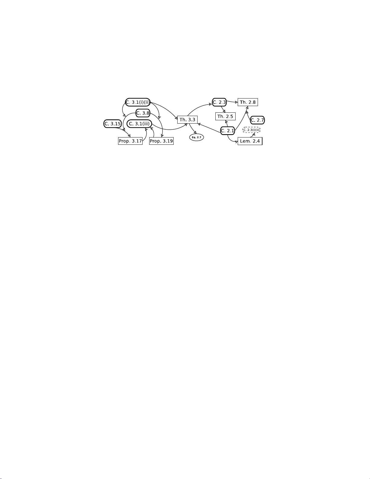
Bernoul li 20 (2), 2014, 545–585 DOI: 10.315 0/12-BEJ 497 Mark o vian sto c hastic appro ximation with expanding pro jections CHRISTOPHE ANDRIEU 1 and MA TTI VIHOLA 2 1 Scho ol of Mathematics, University of Bristol, BS8 1TW, Unite d Kingdom. E-mail: C.Andrieu@brist ol.ac.uk 2 Dep artment of Mathematics and Statistics, University of Jyv¨ askyl¨ a, P. O. Box 35, FI-40014, Finland. E-mail: matti.vihola@iki.ﬁ Sto c hastic approximation is a framew ork unifying many random iterativ e algorithms occurring in a diverse range of app lications. The stabilit y of the pro cess is often diﬃcult to verify in practical app lic ations an d the p rocess may even b e unstable without additional stabilisation techniques. W e study a stochastic appro x imatio n procedu re w ith expanding pro jectio ns simi- lar to Andrad´ ottir [ Op er. R es. 43 (1995) 1037–1048]. W e fo cus o n Marko v ian noise a nd show the stabilit y and conv ergence u nder general conditions. Our framew ork also incorp orates the p oss ibilit y to use a ra ndom step size sequence, w hich allo ws us to consider settings with a non- smooth family of Mark ov k ernels. W e apply the theory to stochastic approximati on exp ectatio n maximisation with particle indep endent Metropolis–Hastings sampling. Keywor ds: exp ectation maximisation; indep enden t Metrop olis–Hastings; particle Marko v chain Mon te Carlo; stability; sto c hastic app ro ximation 1. In tro duction Sto c hastic approximation (SA) is c o ncerned with ﬁnding the z e ros of a function deﬁned on the space Θ ⊂ R d as h ( θ ) := Z X H ( θ, x ) π θ (d x ) , (1.1) where { π θ } θ ∈ Θ is a fa mily of probability distributions on a gener ic measurable space ( X , B ( X )) and H : Θ × X → Θ is a measurable function. In numerous s ituations h b e - hav es like a gradient, suggesting that a recur sion of the type θ i +1 = θ i + γ i +1 h ( θ i ) where ( γ i ) i ≥ 1 is a sequence of nonnega tiv e step sizes decaying to zer o, ca n b e used to ﬁnd the aforementioned r oots. Often in applications, the int egral ( 1.1 ) needs to b e approximated numerically . W e fo cus her e on metho ds relying o n Monte Carlo simulation where sampling exa ctly from This is an electronic reprint of the original article p ublished by the ISI /BS in Bernoul li , 2014, V ol. 20, No. 2, 545–585 . This reprint diﬀers from the original in pagination and typographic detail. 1350-7265 c  2014 ISI/BS 2 C. Andrieu and M. Vihola π θ for any θ ∈ Θ is not p ossible dire ctly and instead Ma rk ov chain Mon te Carlo metho ds are used. Let { P θ } θ ∈ Θ be a family o f Markov trans ition probabilities with statio nary distributions { π θ } θ ∈ Θ , resp ectiv ely . Then, the s ta ndard SA recursio n with Ma rk ovian dynamic is a s follows X i +1 | θ 0 , X 0 , . . . , θ i , X i ∼ P θ i ( X i , · ) , θ i +1 = θ i + γ i +1 H ( θ i , X i +1 ) . Stabilit y of this pro cess is far from o b vious and a signiﬁcant eﬀor t has b een dedicated to its s tudy (e.g., [ 7 ], Section 7.3). Pro blems o ccur in particular when er godicity , a term to b e made more precis e later, of P θ v anishes as θ a pproaches a set of critical v alues denoted ∂ Θ he r eafter. Y ounes [ 30 ], Section 6.3, g iv es an example of a situa tion where the Robbins–Monro algo rithm fails for this reaso n. Cures include pro jection on a ﬁxed set R 0 ⊂ Θ, that is , given a pr o jection mapping Π R 0 : Θ \ R 0 → R 0 , one can deﬁne [ 20 , 21 ] θ ∗ i +1 = θ i + γ i +1 H ( θ i , X i +1 ) , θ i +1 = θ ∗ i +1 I { θ ∗ i +1 ∈ R 0 } + Π R 0 ( θ ∗ i +1 ) I { θ ∗ i +1 / ∈ R 0 } . Pro jection on a ﬁxed s et R 0 might not b e sa tisfactory when for example the lo cation of the zeros of h ( θ ) is not known a priori. It is also p ossible that the pro jection induces spurious a ttr a ctors on the b oundary of R 0 . Adaptive pro jectio ns o vercome these diﬃculties by considering an increasing s e quence of pro jection s ets {R i } i ≥ 0 which forms a covering of Θ. The pr ocess is deﬁned through [ 4 , 1 1 – 13 , 2 8 ] θ ∗ i +1 = θ i + γ i +1 H ( θ i , X i +1 ) , θ i +1 = θ ∗ i +1 I { θ ∗ i +1 ∈ R r i } + Π R 0 ( θ ∗ i +1 ) I { θ ∗ i +1 / ∈ R r i } , r i +1 = r i + I { θ ∗ i +1 / ∈ R r i } , where r i is the indicator of the curre n t repr o jection set and r 0 ≡ 0 . Adaptive pro jections can b e shown to le ad to s table rec ur sions under r ather general conditions. In the case o f a Ma rk ovian noise, one usually mo diﬁes a lso X i +1 so tha t [ 4 ] X i +1 | θ 0 , X 0 , . . . , θ i , X i ∼ P θ i ( X ∗ i , · ) with X ∗ i := I { θ ∗ i ∈ R i − 1 } X i + I { θ ∗ i / ∈ R i − 1 } ˆ Π K 0 ( X i ) , where ˆ Π K 0 : X → K 0 maps X i to a suitable (usually compact) set K 0 ⊂ X . This corre sponds eﬀectively to ‘r estarting’ the pr ocess, with a sma ller step size se q uence and a bigg er feasible set R r i +1 . One ca n sho w that the pro jections o ccur ﬁnitely often under fair ly general conditions, whence the pro cess is ev entually stable [ 4 ]. In practice, this algorithm may be wasteful if {R i } i ≥ 0 or K 0 are ill-deﬁned, and the pro jections o ccur frequently . Markovia n sto chastic appr oximation with exp anding pr oje ctions 3 W e fo cus her e on the study of a diﬀerent stabilising approa ch where pro jection o ccurs on an expanding (with time) sequence of pro jection sets {R i } . Our approa c h is similar to Andrad´ ottir’s [ 1 ]; see also [ 2 6 , 27 ], but we consider a more genera l fra mew or k with t wo ma jor diﬀerences. First, w e fo cus on a Marko v ian noise setting, and second, we allo w the step s iz e sequence, now denoted (Γ i ) i ≥ 1 , to be ra ndo m. 1 Our analysis is inspire d by earlier re la ted work in ada ptiv e Marko v chain Monte Carlo [ 25 ]. The generic algorithm can b e given a s follows. Algorithm 1.1. L et {R i } i ≥ 0 b e subsets of Θ and let the weights (Γ i ) i ≥ 1 b e nonne ga- tive r andom variables. The s t o chastic appr oximation pr o c ess ( θ i , X i ) i ≥ 0 with exp anding pr oje ction s et s {R i } i ≥ 0 is deﬁne d for any starting p oint ( θ 0 , X 0 ) ≡ ( θ , x ) ∈ R 0 × X and r e cursively for i ≥ 0 as fol lows X i +1 |F i ∼ P θ i ( X i , · ) , θ ∗ i +1 = θ i + Γ i +1 H ( θ i , X i +1 ) , θ i +1 = θ ∗ i +1 I { θ ∗ i +1 ∈ R i +1 } + θ pro j i +1 I { θ ∗ i +1 / ∈ R i +1 } , wher e F i stands for t he σ -algebr a gener ate d by θ 0 , X 0 , θ 1 , X 1 , Γ 1 , . . . , θ i , X i , Γ i , and wher e θ pro j i +1 is a σ ( F i , X i +1 , θ ∗ i +1 ) -me asur able r andom va riable taking values in R i +1 . Most common practica l pro jection mec hanisms include θ pro j i +1 := θ i ‘rejecting’ an up date outside the current feasible set, and θ pro j i +1 := Π R i +1 ( θ ∗ i +1 ), where Π R i +1 : Θ \ R i +1 → R i +1 is a measura ble mapping. In words, the ex panding pro jections approa c h only ensur es that θ i is in a feasible set R i but does not in volve potentially ha rmful ‘res tarts’ as is the case with the adap- tive repro jection strategy . Note par ticularly that unlik e with the adaptiv e r epro jections strategy , we need not pro ject X i +1 at all. W e b eliev e that these adv antages c an provide signiﬁcantly b etter r esults in c ertain settings, but this is at the exp ense of req uir ing more when proving the stability and the convergence o f the pro cess. In short, we must be able to co n trol cer tain q ua n titative cr iteria within each feasible s et R i . The random step size s e quence allows one to consider situations where the family of Marko v kernels { P θ } θ ∈ Θ is not necessa rily smo oth in a ma nner that is usually considered in the sto c hastic approximation liter a ture (e.g., [ 8 ]). Other stabilisation techniques in the literature rela ted to our appro ac h include the state-dep enden t av era ging fra mew or k of Y ounes [ 30 ] and a state-dep endent step s iz e sequence of Ka mal [ 19 ]. Particularly the former shar es s imila rities with the pr esen t work, as it als o relie s on quantifying the er godicity rates of Ma rk ov kernels explicitly . O ur stabilisation a pproach diﬀers, how ever, crucia lly from these metho ds, adding only the pro jections to the basic Robbins–Monro algor ithm. W e remark also that our present approach may be used in some situations to prov e the stability and con vergence of an 1 The recen t work of Sharia [ 27 ] includes random step sizes as w ell, but our assumptions on Γ i are completely diﬀerent . 4 C. Andrieu and M. Vihola Figure 1. Road map of the main results and assumptions. unmo diﬁe d Robbins–Monro sto chastic approximation. This is p ossible, lo osely sp eaking, if one can show that pro jections do not o ccur at all with a p ositive proba bilit y; see [ 25 ] for an example o f suc h a situation. W e point out also the w or k [ 6 ] sugg e sting a generic metho d to establis h the stability of unmo diﬁed Markovian Robbins–Monro s to chastic approximation a t the exp ense of more stringent assumptions. Our main results show that the SA pro cess ( θ i ) i ≥ 0 pro duced by our e x panding pr o jec- tions algorithm ‘stays aw ay from ∂ Θ ’ almost surely for a n y starting p oint ( θ , x ) ∈ R 0 × X under conditions on H ( · , · ), { P θ } θ ∈ Θ , ( R i ) i ≥ 0 and (Γ i ) i ≥ 1 . Fig ure 1 summar ises the inter- depe ndency b et ween our v ar io us main conditions and r esults and in order to help the reader we provide a nomenclatur e of some of the c o nstan ts involv ed in App endix D . Section 2 contains tw o fundamental results, Theorems 2.5 and 2 .8 , which b oth establish stability of Alg o rithm 1.1 under abstract noise conditions and the existence of a Lya- punov function satisfying tw o distinct sets of ass umptions which, r oughly sp eaking, a llo w us to tackle ins tabilit y at inﬁnit y or at a ﬁnite p oin t. Section 3 focuses on es tablishing the required nois e conditions with v er iﬁable assumptions on the Mark ov kernels. First, Theorem 3 .3 establishes the a fo remen tioned noise conditio ns under Condition 3.1 , which essentially involv es a tra de-oﬀ b et ween the sequences (Γ i ) i ≥ 0 and ( ξ i ) i ≥ 0 and pro perties of the solution of the Poisson equation related to { P θ } θ ∈ Θ and H ( · , · ). Sec o nd, esse n- tially ass uming geometric ergo dicity , Propo sitions 3.17 and 3 .19 establish the required conditions in the scenar ios where { P θ } θ ∈ Θ depe nds smo othly on θ and wher e it do es not resp ectiv e ly —the latter ca se re q uires the in tro duction of ra ndom step-sizes (Γ i ) i ≥ 0 (see also the comments in the in tr oduction of Section 3.3 ). W e complement our stability results in Section 4 with a discussion on how one c a n use existing r esults in the literature to obtain convergence of ( θ i ) i ≥ 0 to a zero of h . Finally , we apply our theory to a new sto chastic a ppro ximation exp ectation maximisation algo rithm inv olving pa rticle indep enden t Metrop olis–Hastings sampling in Section 5 . 2. General stabilit y results W e deno te throughout the article the probability distribution asso ciated to the pro cess ( θ i , X i ) i ≥ 0 deﬁned in Algorithm 1.1 and starting at ( θ 0 , X 0 ) ≡ ( θ, x ) ∈ Θ × X as P θ ,x ( · ) and the asso ciated exp ectation as E θ ,x [ · ]. F or any subset A ⊂ E of so me space E , we Markovia n sto chastic appr oximation with exp anding pr oje ctions 5 denote A c its complement in E . W e also denote h· , ·i the s tandard inner pro duct and | · | the asso ciated norm on Θ ⊂ R d . W e als o use the notation a ∨ b := max { a , b } and a ∧ b := min { a, b } . The a pproach we develop relies o n the existence o f a Lyapunov function w : Θ → [0 , ∞ ) for the recurs ion o n θ a nd the subs equen t pro of that { w ( θ i ) } is P θ ,x -a.s. under some adequate level. F or any M > 0, we deﬁne the level sets W M := { θ ∈ Θ: w ( θ ) ≤ M } . Our general stability res ults are inspir ed by a pro of due to Benveniste, Me tivie r a nd Pr iouret [ 8 ], Theo rem 17, page 23 9 , but diﬀer in many resp ects as we shall see. W e consider tw o diﬀerent settings co ncerning the wa y w behav es on the b oundary ∂ Θ of Θ . Section 2.1 assumes that lim θ → ∂ Θ w ( θ ) = ∞ , whic h is well suited for example to the case Θ = R a nd ∂ Θ = {−∞ , ∞} . Section 2.2 considers the cas e where w may no t be unbounded, which req uires strong er assumptions on the behaviour o f w . This setting subsumes for example the cas e where Θ ⊂ R and ∂ Θ contains some points on the real line. Both of the scenario s share the following set of assumptions. Condition 2.1. Ther e exists a twic e c ontinuously diﬀer ent iable f unction w : Θ → [0 , ∞ ) such that (i) the Hessian matrix Hess w : Θ → R d × d of w is b ounde d so that C w := sup θ ∈ Θ sup | θ 0 | =1 | Hess w ( θ ) θ 0 | < ∞ , (ii) the pr oje ction sets ar e incr e asing su bsets of Θ , that is, R i ⊂ R i +1 for al l i ≥ 0 , and ˆ Θ := S ∞ i =0 R i ⊂ Θ , (iii) ther e ex ists a c onst ant M 0 > 0 such that for any θ ∈ W c M 0 ∩ ˆ Θ h∇ w ( θ ) , h ( θ ) i ≤ 0 , (iv) the family of r andom variables { θ pro j i } i ≥ 1 satisﬁes for all i ≥ 1 whenever θ ∗ i / ∈ R i θ pro j i ∈ R i and w ( θ pro j i ) ≤ w ( θ ∗ i ) P θ ,x -a.s. , (v) ther e exists c onstants α w , c ∈ [0 , ∞ ) and a non-de cr e asing se qu en c e of c onstants ξ i ∈ [1 , ∞ ) satisfying sup θ ∈R i |∇ w ( θ ) | ≤ cξ α w i for al l i ≥ 0 . R emark 2.2. Co ndition 2.1 (i) Can often b e e stablished by intro ducing a L yapunov function deﬁned through w := ψ ◦ ˜ w , where ψ : [0 , ∞ ) → [0 , ∞ ) is a suitable concave function modifying the v alues of a nother Lyapunov function ˜ w which satisﬁes the drift c o ndition (iii) but do es not hav e ﬁnite second deriv atives; see [ 8 ], Remark o n pag e 23 9. (ii) Is often sa tis ﬁed with ˆ Θ = Θ, but accomo dates a lso pro jections sets which do not cov er Θ, but only certain admiss ible v alues ˆ Θ ( Θ . As an extr eme c a se, this allows to use the present framework to chec k that a ﬁxed pro jection do es no t induce spurious a ttr actors on the b oundary of ˆ Θ. Notice a lso that the function 6 C. Andrieu and M. Vihola H ( θ, x ) a nd the cor r esponding mean ﬁeld h ( θ ) need only b e deﬁned for v a lues θ ∈ ˆ Θ. (iii) Will b e replac ed with a stricter drift in Theor e m 2 .8 , where w is not required to diverge o n the b oundary ∂ ˆ Θ. (iv) Is satisﬁed triv ially by the choices θ pro j i := θ i − 1 and θ pro j i := Π R i ( θ ∗ i ), if the pro jec- tion sets are deﬁned a s the level s ets of the Lyapunov function, tha t is R i := W M i for some M i > 0. In the Mar k ovian cas e , the pro jections are assumed to satisfy an a dditio nal contin uity condition; see Theorem 3.3 . (v) Inv olves in pr actice a se quence that g ro ws a t mo st at a r ate ξ i := i ∨ 1 , with some power α w ∈ [0 , 1). The sequence ξ i plays a central ro le a lso in controlling the ergo dicit y rate of the Ma rk ov chain in R i ; see Remar k 3.2 . Hereafter, w e denote the ‘centred’ v er sion of H as ¯ H ( θ, x ) := H ( θ, x ) − h ( θ ) . F or the stability res ults, we shall introduce the following general conditio n on the no ise s e quence. In general terms, it is related to the rate at which { θ i } may appro ac h ∂ ˆ Θ in relation to the growth of | H ( θ , x ) | and the loss of ergo dicity of { P θ } . Establishing prac tica l and realistic co nditions under which this a s sumption holds will be the topic of Section 3 . Condition 2. 3. F or any ( θ, x ) ∈ R 0 × X it holds that (i) P θ ,x  lim i →∞ Γ i +1 |∇ w ( θ i ) | · | H ( θ i , X i +1 ) | = 0  = 1 , (ii) E θ ,x " ∞ X i =0 Γ 2 i +1 | H ( θ i , X i +1 ) | 2 # < ∞ , (iii) E θ ,x " sup k ≥ 0      k X i =0 Γ i +1 h∇ w ( θ i ) , ¯ H ( θ i , X i +1 ) i      # < ∞ . In what follows, we sha ll fo cus o n a single condition implying Condition 2.3(i) and (ii) . It is slightly more stringent, but more c on venien t to ch eck in prac tice . Lemma 2.4. Supp ose Condition 2.1 holds and E θ ,x " ∞ X i =0 Γ 2 i +1 ξ 2 α w i | H ( θ i , X i +1 ) | 2 # < ∞ . (2.1) Then, Condition 2.3 (i) and (ii) ho ld. Pro of. Note ﬁrst that Co ndition 2.3(ii) holds trivially , b ecause ξ 2 α w i ≥ 1 . F or Condition 2.3(i) , co nsider E θ ,x " ∞ X i =0 (Γ i +1 |∇ w ( θ i ) | · | H ( θ i , X i +1 ) | ) 2 # ≤ c 2 E θ ,x " ∞ X i =0 Γ 2 i +1 ξ 2 α w i | H ( θ i , X i +1 ) | 2 # .  Markovia n sto chastic appr oximation with exp anding pr oje ctions 7 2.1. Un b ounded Ly apuno v function When lim θ → ∂ ˆ Θ w ( θ ) = ∞ , it is enough to show that the s e quence w ( θ i ) is b ounded in order to ensure the stability of θ i . Theorem 2.5. Assume Conditions 2.1 and 2. 3 hold . Then, for any ( θ , x ) ∈ R 0 × X P θ ,x  lim sup i →∞ w ( θ i ) < ∞  = 1 . Pro of. T o show the P θ ,x -a.s. b oundedness of { w ( θ i ) } we ﬁx ( θ , x ) ∈ R 0 × X and introduce the following quantities. Let M 0 < M 1 < · · · < M n → ∞ be an increa sing sequence tending to inﬁnity and cons ide r the level sets W M i ⊂ Θ . W e assume tha t M 0 is chosen lar ge enough so that θ 0 = θ ∈ W M 0 . F o r any n ≥ 0 , we deﬁne the ﬁrst exit time of θ i from the level set W M n as σ n := inf { i ≥ 0 : θ i / ∈ W M n } , with the usual conv ention that inf { ∅ } = ∞ . F or any n ≥ 0 , we deﬁne the time following the last exit of θ i from W M 0 befo re σ n as τ n := 1 + sup { i ≤ σ n : θ i ∈ W M 0 } , which is ﬁnite at least whenever σ n is ﬁnite by our a s sumption that θ 0 ∈ W M 0 . With these deﬁnitions, the claim holds once we show that lim n →∞ P θ ,x ( σ n < ∞ ) = 0. T o b egin with, deﬁne for n ≥ 1 the following sets characterising the jumps o ut o f W M 0 D n :=  I { τ n < ∞} [ w ( θ τ n ) − w ( θ τ n − 1 )] ≤ M n − M 0 2  . W e ﬁrst show that lim n →∞ P θ ,x ( D n ) = 1 . Clearly ˜ D n :=  sup i ≥ 0 [ w ( θ i +1 ) − w ( θ i )] ≤ M n − M 0 2  ⊂ D n (2.2) and since M n → ∞ , one has { sup i ≥ 0 [ w ( θ i +1 ) − w ( θ i )] < ∞} = S ∞ n =1 ˜ D n . Lemma 2.6 shows that 1 = P θ ,x ( S ∞ n =1 ˜ D n ) = lim n →∞ P θ ,x ( ˜ D n ) ≤ lim n →∞ P θ ,x ( D n ) b ecause ˜ D n is a n increasing sequence a nd by ( 2.2 ), r espectively . Now, it rema ins to focus o n pr o ving that lim n →∞ P θ ,x ( D n ∩ { σ n < ∞} ) = 0 . In or der to achiev e this observe ﬁrst that w ( θ σ n ) − w ( θ τ n − 1 ) ≥ M n − M 0 on { σ n < ∞} , implying that on D n ∩ { σ n < ∞} , w ( θ σ n ) − w ( θ τ n ) = w ( θ σ n ) − w ( θ τ n − 1 ) − [ w ( θ τ n ) − w ( θ τ n − 1 )] ≥ M n − M 0 2 . 8 C. Andrieu and M. Vihola This allows us to deduce the following b ound P θ ,x ( D n ∩ { σ n < ∞} ) = E θ ,x [ I { D n ∩ { σ n < ∞}} ] ≤ E θ ,x  I { D n ∩ { σ n < ∞}} w ( θ σ n ) − w ( θ τ n ) (1 / 2)( M n − M 0 )  ≤ 2 M n − M 0 E θ ,x [ I { σ n < ∞} [ w ( θ σ n ) − w ( θ τ n )]] . Since M n → ∞ , the pr oof will be ﬁnished once we s ho w that sup n ≥ 0 E θ ,x [ I { σ n < ∞} [ w ( θ σ n ) − w ( θ τ n )]] < ∞ . (2.3) Thanks to Co ndition 2.1(iv) , we have for a n y i ≥ 0 that w ( θ i +1 ) ≤ w ( θ ∗ i +1 ) and conse- quently w ( θ i +1 ) − w ( θ i ) ≤ Γ i +1 h∇ w ( θ i ) , h ( θ i ) i + Γ i +1 h∇ w ( θ i ) , ¯ H ( θ i , X i +1 ) i + Γ 2 i +1 C w 2 | H ( θ i , X i +1 ) | 2 . So in par ticula r, since h∇ w ( θ i ) , h ( θ i ) i ≤ 0 whenev er θ i ∈ W c M 0 , I { σ n < ∞} [ w ( θ σ n ) − w ( θ τ n )] = I { σ n < ∞} σ n − 1 X i = τ n [ w ( θ i +1 ) − w ( θ i )] ≤ I { σ n < ∞} σ n − 1 X i = τ n Γ i +1 h∇ w ( θ i ) , ¯ H ( θ i , X i +1 ) i + Γ 2 i +1 C w 2 | H ( θ i , X i +1 ) | 2 ! . Recall the following estimate for partial sums      k X i = j a i      =      k X i =0 a i − j − 1 X i =0 a i      ≤      k X i =0 a i      +      j − 1 X i =0 a i      ≤ 2 sup k ≥ 0      k X i =0 a i      , (2.4) implying in our case that 1 2 I { σ n < ∞} [ w ( θ σ n ) − w ( θ τ n )] ≤ I { σ n < ∞} sup k ≥ 0      k X i =0 Γ i +1 h∇ w ( θ i ) , ¯ H ( θ i , X i +1 ) i      + ∞ X i =0 Γ 2 i +1 C w 2 | H ( θ i , X i +1 ) | 2 ! . Now, Co ndition 2.3(ii) and (iii) imply ( 2.3 ) allowing us to co nclude.  Markovia n sto chastic appr oximation with exp anding pr oje ctions 9 Lemma 2.6. Under Condition 2.3 we ha ve, P θ ,x -almost su r ely lim sup i →∞ [ w ( θ i +1 ) − w ( θ i )] ≤ 0 , (2.5) sup i ≥ 0 [ w ( θ i +1 ) − w ( θ i )] < ∞ . (2.6) Pro of. W e ﬁrst prov e that lim i →∞ | w ( θ ∗ i +1 ) − w ( θ i ) | = 0, P θ ,x -a.s. By a T aylor expansion, we g et | w ( θ ∗ i +1 ) − w ( θ i ) | ≤ |∇ w ( θ i ) | · | Γ i +1 H ( θ i , X i +1 ) | + Γ 2 i +1 C w | H ( θ i , X i +1 ) | 2 . The terms on the right conv er ge to zero P θ ,x -a.s. by Condition 2.3(i) and (ii) , resp ectively . Now, ( 2.5 ) follows since by Condition 2.1(iv) w ( θ i +1 ) − w ( θ i ) ≤ w ( θ ∗ i +1 ) − w ( θ i ). W e conclude by noting that ( 2.6 ) follows dir ectly from ( 2.5 ).  2.2. Bounded Ly apuno v function In the previous section, the Lyapunov function satisﬁed lim θ → ∂ ˆ Θ w ( θ ) = ∞ . If this is no t the case, we need to replace Co ndition 2.1(iii) with a more stringent condition quantifying the drift outside W M 0 , while not requir ing lim θ → ∂ ˆ Θ w ( θ ) = ∞ . Condition 2. 7. The Lyapunov fun ction and the step size se quen c e satisfy δ i := inf θ ∈R i \W M 0 −h∇ w ( θ ) , h ( θ ) i > 0 and ∞ X i =1 Γ i δ i = ∞ P θ ,x -almost su r ely . Theorem 2.8. Assum e Conditions 2.1 , 2.3 and 2.7 hold, and in addition that the fol- lowing c ondition on the noise ho lds lim m →∞ sup k>m      k X i = m Γ i +1 h∇ w ( θ i ) , ¯ H ( θ i , X i +1 ) i      = 0 . (2.7) Then for any M > M 0 , the tails of t he tra je ctories of { θ i } ar e eventual ly c ontaine d within W M P θ ,x -a.s., that is, P θ ,x  [ m ≥ 0 \ n ≥ m { θ n ∈ W M }  = 1 . Pro of. W e ﬁr s t s how that θ n m ust visit W M 0 inﬁnitely often P θ ,x -a.s., in o ther words P θ ,x  [ m ≥ 1 \ n ≥ m { θ n / ∈ W M 0 }  = 0 . (2.8) 10 C. Andrieu and M. Vihola F or any m ≥ 0 , we deﬁne the hitting times κ m := inf { i > m : θ i ∈ W M 0 } and notice that [ m ≥ 1 \ n ≥ m { θ n / ∈ W M 0 } = [ m ≥ 1 { θ m / ∈ W M 0 } ∩ { κ m = ∞} . Recall tha t for any i ≥ 0 w ( θ i +1 ) − w ( θ i ) ≤ Γ i +1 h∇ w ( θ i ) , h ( θ i ) i + Γ i +1 h∇ w ( θ i ) , ¯ H ( θ i , X i +1 ) i + Γ 2 i +1 C w 2 | H ( θ i , X i +1 ) | 2 . So in par ticula r, a nd thanks to Condition 2.7 , for n > m I { θ m / ∈ W M 0 } [ w ( θ n ∧ κ m ) − w ( θ m )] = I { θ m / ∈ W M 0 } ( n ∧ κ m ) − 1 X i = m I { θ i / ∈ W M 0 } [ w ( θ i +1 ) − w ( θ i )] ≤ I { θ m / ∈ W M 0 } ( n ∧ κ m ) − 1 X i = m Γ i +1  − δ i + h∇ w ( θ i ) , ¯ H ( θ i , X i +1 ) i + Γ i +1 C w 2 | H ( θ i , X i +1 ) | 2  . F rom this, w e obtain the follo wing inequality ho lding P θ ,x -a.s. on { θ m / ∈ W M 0 } for an y n > m E θ ,x " I { κ m = ∞} n − 1 X i = m Γ i +1 δ i    F m # − w ( θ m ) ≤ E θ ,x " I { κ m = ∞} n − 1 X i = m Γ i +1 h∇ w ( θ i ) , ¯ H ( θ i , X i +1 ) i (2.9) + Γ 2 i +1 C w 2 | H ( θ i , X i +1 ) | 2    F m # . Using this inequality , we shall see that for a n y m > 0 P θ ,x ( { θ m / ∈ W M 0 } ∩ { κ m = ∞} ) = 0 . (2.10) Suppo se the co n trar y , P θ ,x ( { θ m / ∈ W M 0 } ∩ { κ m = ∞} ) > 0 . Then, b ecause of Condition 2.7 , we observe that the conditiona l exp ectation on the le ft hand side of ( 2 .9 ) necess a rily tends to inﬁnity almost surely a s n → ∞ . Denote then the conditional exp ectation on the right hand side o f ( 2.9 ) by E ( m,n ) θ ,x . As in the pro of of Theo rem 2 .5 , we hav e the following upper b ound E θ ,x [ E ( m,n ) θ ,x ] ≤ E θ ,x " sup k ≥ 0      k X i =0 Γ i +1 h∇ w ( θ i ) , ¯ H ( θ i , X i +1 ) i      + ∞ X i =0 Γ 2 i +1 C w 2 | H ( θ i , X i +1 ) | 2 # , Markovia n sto chastic appr oximation with exp anding pr oje ctions 11 which is ﬁnite by Condition 2.3 and indep enden t of m and n . By letting n → ∞ w e end up with a contradiction, unless ( 2.10 ) holds . Co ns equen tly , the even t [ m ≥ 1 { θ m / ∈ W M 0 } ∩ { κ m = ∞} has null proba bilit y and we o btain ( 2.8 ). W e now s how that for any ﬁxed M > M 0 P θ ,x  [ m ≥ 0 \ n ≥ m { θ n ∈ W M }  = 1 . W e are go ing to a pply Lemma 2.9 below with δ = M − M 0 > 0 to the even ts A m = { θ m ∈ W M 0 } ∩ [ k>m { θ k / ∈ W M } , and denote B m := { θ m ∈ W M 0 } \ A m = { θ m ∈ W M 0 } ∩ \ k>m { θ k ∈ W M } . W e may wr ite \ n ≥ 1 [ m ≥ n { θ m ∈ W M 0 } = \ n ≥ 1 [ m ≥ n A m ∪ B m = \ n ≥ 1  [ m ≥ n A m  ∪  [ m ≥ n B m  . Now, since S m ≥ n A m and S m ≥ n B m are bo th decreasing events with resp ect to n → ∞ , we have 1 = lim n →∞ P θ ,x  [ m ≥ n { θ m ∈ W M 0 }  = lim n →∞  P θ ,x  [ m ≥ n A m  + P θ ,x  [ m ≥ n B m  − P θ ,x  [ m ≥ n A m ∩ [ m ≥ n B m  . By L e mma 2.9 , lim n →∞ P θ ,x ( S m ≥ n A m ) = 0 , so we end up with lim n →∞ P θ ,x ( S m ≥ n B m ) = 1, implying the claim.  Lemma 2.9. Assume t he c onditions of The or em 2.8 , let δ > 0 and denote A m := { θ m ∈ W M 0 } ∩ [ k>m { θ k / ∈ W M 0 + δ } . Then, lim n →∞ P θ ,x ( S m ≥ n A m ) = 0 . 12 C. Andrieu and M. Vihola Pro of. Deﬁne the random times σ m := inf { i > m : θ i / ∈ W M 0 + δ } a nd τ m := s up { i ∈ [ m, σ m ): θ i ∈ W M 0 } + 1 , b oth ﬁnite on A m . Recall that on { θ i ∈ W c M 0 } we have w ( θ i +1 ) − w ( θ i ) ≤ Γ i +1 h∇ w ( θ i ) , ¯ H ( θ i , X i +1 ) i + Γ 2 i +1 C w 2 | H ( θ i , X i +1 ) | 2 , so o n A m we may b ound w ( θ σ m ) − w ( θ τ m ) ≤ σ m − 1 X i = τ m Γ i +1 h∇ w ( θ i ) , ¯ H ( θ i , X i +1 ) i + Γ 2 i +1 C w 2 | H ( θ i , X i +1 ) | 2 ≤ 2 sup k>m      k X i = m Γ i +1 h∇ w ( θ i ) , ¯ H ( θ i , X i +1 ) i      + ∞ X i = m Γ 2 i +1 C w 2 | H ( θ i , X i +1 ) | 2 =: C m by a similar ar g umen t as in ( 2.4 ). On A m one clearly has w ( θ σ m ) − w ( θ τ m − 1 ) > δ , implying that C m + w ( θ τ m ) − w ( θ τ m − 1 ) > δ . W e deduce that ˜ A m := n C m + sup i ≥ m [ w ( θ i +1 ) − w ( θ i )] > δ o ⊃ A m . The sets ˜ A m are clear ly decrea sing with res pect to m and lim m →∞ P θ ,x ( ˜ A m ) = 0 by Lemma 2.6 and b ecause Co ndition 2.3(ii) and ( 2.7 ) imply lim m →∞ C m = 0. This con- cludes the pro of, b ecause S m ≥ n A m ⊂ S m ≥ n ˜ A m = ˜ A n .  3. V erifying noise conditions The aim of this section is to provide veriﬁable co nditions which will imply the co nditions of the stability theor ems in Section 2 . W e pr oceed progressively and start by a general result in Theorem 3.3 which ensures bo th Condition 2.3 and that in ( 2.7 ) ho ld given a set of abstract conditions inv olving some exp ectations as well as pro perties of the solutio ns of the Poisson equatio n. Condition 3.1 , required in Theorem 3.3 , shall b e v er iﬁe d in detail b elo w for a family of geometr ically er godic Marko v k er nels. In Section 3.1 , we ﬁrst g ather general known results related to Condition 3.1(ii) and (iii) . In Se c tion 3.2 , w e co nsider the case where the mapping θ → P θ is H¨ older contin uo us, which allows us to es tablish Condition 3.1(iv) . In Section 3.3 , we co nsider the cas e wher e the a foremen tioned H¨ older contin uity may not hold, and a contin uity is enforce d b y using a random step size seq uence, a llo wing us to recov e r Condition 3.1(iv) in such situa tions. Condition 3.1. Condition 2.1 holds with c onst ants ( ξ i ) i ≥ 0 and α w ∈ (0 , ∞ ) . F or al l θ ∈ ˆ Θ , the solut io n g θ : X → Θ to the Poisson e quation g θ ( x ) − P θ g θ ( x ) ≡ ¯ H ( θ, x ) ex ists and for al l i ≥ 0 the step size Γ i +1 is indep endent of F i and X i +1 . Mor e over, t her e Markovia n sto chastic appr oximation with exp anding pr oje ctions 13 exist a me asur able function V : X → [1 , ∞ ) and c onstant s c < ∞ , β H , β g ∈ [0 , 1 / 2] and α g , α H , α V ∈ [0 , ∞ ) such that for al l ( θ , x ) ∈ R 0 × X (i) sup θ ∈R i | H ( θ, x ) | ≤ cξ α H i V β H ( x ) , (ii) E θ ,x [ V ( X i )] ≤ cξ α V i V ( x ) , (iii) sup θ ∈R i [ | g θ ( x ) | + | P θ g θ ( x ) | ] ≤ cξ α g i V β g ( x ) , (iv) ∞ X i =1 E [Γ i +1 ] ξ α w i E θ ,x [ | P θ i g θ i ( X i ) − P θ i − 1 g θ i − 1 ( X i ) | ] < ∞ , (v) ∞ X i =1 E [Γ 2 i ] ξ 2 α w +2(( α H + β H α V ) ∨ ( α g + β g α V )) i < ∞ , (vi) ∞ X i =1 E [Γ i +1 Γ i ] ξ α H + α g +( β H + β g ) α V i < ∞ , (vii) ∞ X i =1 | E [Γ i +1 − Γ i ] | ξ α w + α g + β g α V i < ∞ , wher e we write E := E θ ,x whenever the ex p e ct atio n do es not dep end on θ and x . R emark 3.2. These a ssumptions call for v arious comments of prac tical relev ance to the actual implemen tation of the alg o rithm with expanding pro jections. Once H ( · , · ) a nd { P θ } θ ∈ Θ are ch osen the user is left with the choice of ( ξ i ) i ≥ 0 and (Γ i ) i ≥ 0 , whic h must in par ticular s a tisfy the summabilit y co nditions a bov e . F o r the purp ose of eﬃciency we would like ( ξ i ) i ≥ 0 to gr o w as fast a s po ssible, as we may o therwise slow co n vergence down. A common choice for the step-size sequence is Γ i = ci − η for so me co nstan ts c ∈ (0 , ∞ ) and η ∈ (1 / 2 , 1 ] – this implies a req uired condition to establish co n vergence. The sequence ( ξ i ) i ≥ 0 is determined b y the use r through the choice of the sequence of repr o jection sets ( R i ) i ≥ 0 and we po in t out that the co nstan ts α H , α V and α g t ypically dep end on that choice (whereas β H and β g t ypically do not). W e show how these constants c a n b e obtained from the pr operties of { P θ } θ ∈ Θ in Sections 3.1 – 3.3 . Now if ( ξ i ) i ≥ 0 is increasing at a rate slower than an y pow er sequence, for example of the order log i or i (log i ) − p for some p ∈ (0 , 1), then it is ea s y to see that the summability conditions (v) – (vii) are alwa y s satisﬁed. In the situation where ξ i = i p for p ∈ (0 , 1], then the conditions (v) – (vii) r equire stricter a ssumptions on η and the co nstan ts α H , α V , α g , β H and β g which may not be satisﬁable. W e howev er point out a p ossible sub-optimalit y o f the results s ta ted ab ov e. Indeed, in or der to simplify presen tation we hav e decided to q ua n tify the g ro wth o f the v arious quantities inv o lv ed in the algo rithm in terms of pow er s of ( ξ i ) i ≥ 0 only , wher eas other scales may b e p ossible, such a s lo g ( ξ i ), in which case so me of the constants α H , α V or α g may be taken a rbitrarily small in the statement a bov e . It is also p ossible to revisit our pro ofs with such mor e precis e estimates and o btain a se t of weak er as sumptions. In practice, the conditions (iii) and (iv) add more req uiremen ts which a re inter-related with (v) – (vii) ; Pr opositio ns 3.17 and 3 .19 summar ise the co nditions when θ 7→ P θ ad- 14 C. Andrieu and M. Vihola mits a H¨ older-contin uit y , and when a random step size sequence is used to satisfy (iv) , resp ectiv e ly . App endix D contains a summary of the related constants. Theorem 3.3. Supp ose Conditions 2.1 and 3.1 hold and for al l i ≥ 0 the pr oje ctions satisfy | θ i +1 − θ i | ≤ | θ ∗ i +1 − θ i | . T hen, for al l ( θ , x ) ∈ R 0 × X , E θ ,x " ∞ X i =0 Γ 2 i +1 ξ 2 α w i | H ( θ i , X i +1 ) | 2 # < ∞ , (3.1) lim m →∞ E θ ,x " sup n ≥ m      n X i = m Γ i +1 h∇ w ( θ i ) , ¯ H ( θ i , X i +1 ) i      # = 0 . (3.2) Pro of. Throughout the proo f, C denotes a constant w hich may have a diﬀerent v a lue upo n each app earance. F or ( 3.1 ), we may use Condition 3.1(i) and (ii) with Jensen’s inequality to obta in E θ ,x " ∞ X i =0 Γ 2 i +1 ξ 2 α w i | H ( θ i , X i +1 ) | 2 # ≤ C ∞ X i =0 E [Γ 2 i +1 ] ξ 2 α w +2 α H i E θ ,x [ V 2 β H ( X i +1 )] ≤ C V 2 β H ( x ) ∞ X i =0 E [Γ 2 i +1 ] ξ 2 α w +2 α H +2 β H α V i , where the sum conv erg es by Condition 3.1(v) . Consider then ( 3.2 ), and deno te the partial sums for n ≥ m ≥ 1 as A m,n := n X i = m Γ i +1 h∇ w ( θ i ) , ¯ H ( θ i , X i +1 ) i . Since ¯ H ( θ i , X i +1 ) = g θ i ( X i +1 ) − P θ i g θ i ( X i +1 ), we may wr ite Γ i +1 h∇ w ( θ i ) , ¯ H ( θ i , X i +1 ) i = Γ i +1 h∇ w ( θ i ) , g θ i ( X i +1 ) − P θ i g θ i ( X i ) i + Γ i +1 h∇ w ( θ i ) , P θ i g θ i ( X i ) − P θ i − 1 g θ i − 1 ( X i ) i + Γ i +1 h∇ w ( θ i ) , P θ i − 1 g θ i − 1 ( X i ) − P θ i g θ i ( X i +1 ) i , where the las t ter m can be written as Γ i +1 h∇ w ( θ i ) , P θ i − 1 g θ i − 1 ( X i ) − P θ i g θ i ( X i +1 ) i = Γ i +1 h∇ w ( θ i ) − ∇ w ( θ i − 1 ) , P θ i − 1 g θ i − 1 ( X i ) i + Γ i h∇ w ( θ i − 1 ) , P θ i − 1 g θ i − 1 ( X i ) i − Γ i +1 h∇ w ( θ i ) , P θ i g θ i ( X i +1 ) i + (Γ i +1 − Γ i ) h∇ w ( θ i − 1 ) , P θ i − 1 g θ i − 1 ( X i ) i . Markovia n sto chastic appr oximation with exp anding pr oje ctions 15 When summing up, the middle term o n the rig h t is telescoping , so in total we may write A m,n = P 5 k =1 R k m,n where R 1 m,n := n X i = m Γ i +1 h∇ w ( θ i ) , g θ i ( X i +1 ) − P θ i g θ i ( X i ) i , R 2 m,n := n X i = m Γ i +1 h∇ w ( θ i ) , P θ i g θ i ( X i ) − P θ i − 1 g θ i − 1 ( X i ) i , R 3 m,n := n X i = m Γ i +1 h∇ w ( θ i ) − ∇ w ( θ i − 1 ) , P θ i − 1 g θ i − 1 ( X i ) i , R 4 m,n := Γ m h∇ w ( θ m − 1 ) , P θ m − 1 g θ m − 1 ( X m ) i − Γ n +1 h∇ w ( θ n ) , P θ n g θ n ( X n +1 ) i , R 5 m,n := n X i = m (Γ i +1 − Γ i ) h∇ w ( θ i − 1 ) , P θ i − 1 g θ i − 1 ( X i ) i . W e sha ll show tha t ( 3.2 ) ho lds for e ac h o f these ﬁve terms in turn, which is suﬃcient to yield the claim. Notice that { R 1 m,i } n i = m is a martingale with resp ect to the ﬁltra tion {F i } n i = m , whence E θ ,x [ | R 1 m,n | 2 ] = n X i = m E θ ,x [Γ 2 i +1 |h∇ w ( θ i ) , g θ i ( X i +1 ) − P θ i g θ i ( X i ) i| 2 ] ≤ C n X i = m ξ 2 α w i E [Γ 2 i +1 ] E θ ,x [ | g θ i ( X i +1 ) | 2 + | P θ i g θ i ( X i ) | 2 ] ≤ C n X i = m ξ 2 α w +2 α g i E [Γ 2 i +1 ] E θ ,x [ V 2 β g ( X i +1 ) + V 2 β g ( X i )] ≤ C V 2 β g ( x ) n X i = m ξ 2 α w +2 α g +2 β g α V i +1 E [Γ 2 i +1 ] , by the fact that Γ i +1 is indep enden t of F i and X i +1 , Condition 2.1(v) , Condition 3.1(ii) and (iii) . Now, Jensen’s and Doo b’s inequality imply  E θ ,x h sup n ≥ m | R 1 m,n | i 2 ≤ E θ ,x h sup n ≥ m | R 1 m,n | 2 i ≤ C V 2 β g ( x ) ∞ X i = m ξ 2 α w +2 α g +2 β g α V i +1 E [Γ 2 i +1 ] . This y ie lds lim m →∞ E θ ,x [sup n ≥ m | R 1 m,n | ] = 0, b ecause the term o n the r igh t tends to zer o as m → ∞ by Conditio n 3.1(v) . 16 C. Andrieu and M. Vihola F or the s econd term R 2 m,n , we may simply write E θ ,x h sup n ≥ m | R 2 m,n | i ≤ E θ ,x " ∞ X i = m | Γ i +1 h∇ w ( θ i ) , P θ i g θ i ( X i ) − P θ i − 1 g θ i − 1 ( X i ) i| # ≤ C ∞ X i = m ξ α w i E [Γ i +1 ] E θ ,x [ | P θ i g θ i ( X i ) − P θ i − 1 g θ i − 1 ( X i ) | ] , which co n verges to zero as m → ∞ by Condition 3.1(iv) . Now w e inspect R 3 m,n . First, since the Hessian is b ounded as in Condition 2.1(i) , w e hav e |∇ w ( θ i ) − ∇ w ( θ i − 1 ) | ≤ C w | θ i − θ i − 1 | ≤ C w | θ ∗ i − θ i − 1 | = C w Γ i | H ( θ i − 1 , X i ) | ≤ C w ξ α H i Γ i V β H ( X i ) , and co nsequen tly E θ ,x h sup n ≥ m | R 3 m,n | i ≤ C ∞ X i = m E [Γ i +1 Γ i ] ξ α g + α H i E θ ,x [ V β g + β H ( X i )] ≤ C V β g + β H ( x ) ∞ X i = m E [Γ i +1 Γ i ] ξ α g + α H +( β g + β H ) α V i , by Co ndition 3.1(i) , (ii) a nd (iii) . The claim follows for R 3 m,n by Co ndition 3.1(vi) . Let us then fo cus on R 4 m,n . W e hav e for any i ≥ m | Γ i h∇ w ( θ i − 1 ) , P θ i − 1 g θ i − 1 ( X i ) i| ≤ C Γ i ξ α w + α g i V β g ( X i ) . Now we hav e E θ ,x h sup n ≥ m | R 4 m,n | 2 i ≤ C ∞ X i = m ξ 2 α w +2 α g i E [Γ 2 i ] E θ ,x [ V 2 β g ( X i )] ≤ C V 2 β g ( x ) ∞ X i = m ξ 2 α w +2 α g +2 β g α V i E [Γ 2 i ] , so ( 3.2 ) ho lds for R 4 m,n by Condition 3.1(v) . W e shall a pply Lemma 3.4 b elow for the la st ter m R 5 m,n , with Z i := Γ i and B i − 1 := h∇ w ( θ i − 1 ) , P θ i − 1 g θ i − 1 ( X i ) i with | B i − 1 | ≤ C ξ α w + α g i − 1 V β g ( X i ) . Markovia n sto chastic appr oximation with exp anding pr oje ctions 17 By the indep endence of Γ i +1 and Γ i , and b ecause ξ i +1 ≥ ξ i ≥ ξ i − 1 , we easily establish the required b ounds ∞ X i =1 V ar(Γ i +1 − Γ i ) E θ ,x [ B 2 i − 1 ] ≤ C V 2 β g ( x ) ∞ X i =1 E [Γ 2 i ] ξ 2 α w +2 α g +2 β g α V i < ∞ , ∞ X i =1 | E [Γ i +1 − Γ i ] | E [ | B i − 1 | ] ≤ C V β g ( x ) ∞ X i =1 | E [Γ i +1 − Γ i ] | ξ α w + α g + β g α V i < ∞ , by Co ndition 3.1(v) and (vii) , resp ectiv ely .  Lemma 3. 4. L et {G i } i ≥ 0 b e a ﬁltr ation and for al l i ≥ 0 let B i and Z i b e G i -adapte d r andom variables so that Z i is indep endent of G i − 1 and ∞ X i =1 V ar( Z i +1 − Z i ) E [ B 2 i − 1 ] < ∞ and ∞ X i =1 | E [ Z i +1 − Z i ] | E [ | B i − 1 | ] < ∞ . Then, lim m →∞ E " sup n ≥ m      n X i = m ( Z i +1 − Z i ) B i − 1      # = 0 . Pro of. Suppose for now that m is even and n o dd and deno te m = 2 ¯ m and n = 2 ¯ n + 1. W rite the sum n X i = m ( Z i +1 − Z i ) B i − 1 = ¯ n X j = ¯ m ( Z 2 j +1 − Z 2 j ) B 2 j − 1 + ¯ n X k = ¯ m ( Z 2 k +2 − Z 2 k +1 ) B 2 k . (3.3) W e shall ﬁrst show that the claim holds for the ﬁr st term on the right. Denote ¯ G j = G 2 j +1 , ¯ Z j = Z 2 j +1 − Z 2 j and ¯ B j − 1 = B 2 j − 1 . Obser v e tha t E [ ¯ Z j | ¯ G j − 1 ] = E [ ¯ Z j ] and write ¯ n X j = ¯ m ( Z 2 j +1 − Z 2 j ) B 2 j − 1 = ¯ n X j = ¯ m ( ¯ Z j − E [ ¯ Z j ]) ¯ B j − 1 + ¯ n X j = ¯ m E [ ¯ Z j ] ¯ B j − 1 . Now, the ﬁrst term on the rig h t-hand side is a martingale with resp ect to ¯ G j , and so by Do o b’s inequality and by a ssumption E " sup ¯ n ≥ ¯ m ¯ n X j = ¯ m ( ¯ Z j − E [ ¯ Z j ]) ¯ B j − 1 ! 2 # ≤ 4 ∞ X j = ¯ m V ar( ¯ Z j ) E [ ¯ B 2 j − 1 ] ¯ m →∞ − − − − → 0 . F or the s econd term, by assumption E " sup ¯ n ≥ ¯ m      ¯ n X j = ¯ m E [ ¯ Z j ] ¯ B j − 1      # ≤ ∞ X j = ¯ m | E [ ¯ Z j ] | E [ | ¯ B j − 1 | ] ¯ m →∞ − − − − → 0 . 18 C. Andrieu and M. Vihola The sa me arguments apply also for the sec o nd term on the rig h t-hand side of ( 3.3 ), a nd for a n y in tegers m ≥ n ≥ 1 , by a change of the indices.  3.1. Geometrically ergo dic Mark ov kernels In this section, we foc us on the scenario where for any θ ∈ Θ the kernel P θ is geometrically ergo dic. This condition is satisﬁed by numerous Markov chains of pra ctical interest, see for example, [ 17 , 18 , 22 ] and r eferences therein. This s ection gathers together s ta ndard results abo ut the reg ularit y of the solutions to the Poisson equatio n (s e e , e.g., [ 3 , 4 ]). Throughout this s e ction, suppo se V : X → [1 , ∞ ) is a ﬁxed meas urable function. W e shall denote the V -norm of a measura ble function f : X → R d by k f k V := sup x | f ( x ) | /V ( x ). W e a lso as sume that for ea c h θ ∈ ˆ Θ, the Mar kov kernel P θ admits a unique inv a rian t probability measure π θ . Condition 3.5. F or any r ∈ (0 , 1] and any θ ∈ ˆ Θ , ther e exist c onst ant s M θ ,r ∈ [0 , ∞ ) and ρ θ ,r ∈ (0 , 1 ) , such that for any function k f k V r < ∞ | P k θ ( x, f ) − π θ ( f ) | ≤ V r ( x ) k f k V r M θ ,r ρ k θ ,r for al l k ≥ 0 and al l x ∈ X . Having Condition 3.5 one can b ound the V r -norm o f the solutions of the Poisson equa- tion, making the dependence o n θ explicit. This r esult is a restatemen t of [ 3 ], Prop osi- tion 3, in quantitativ e form; we pr o vide it here for the r eader’s conv enie nc e . Prop osition 3.6. Assume Condition 3.5 holds. Then, for any fun ct io n k f k V r < ∞ , the functions g θ : X → R d deﬁne d for all θ ∈ ˆ Θ by g θ ( x ) := ∞ X k =0 [ P k θ f ( x ) − π θ ( f )] exist, solve the Poisson e qu ation g θ ( x ) − P θ g θ ( x ) ≡ f ( x ) − π θ ( f ) , and satisfy the b ound k g θ k V r ∨ k P θ g θ k V r ≤ M θ ,r (1 − ρ θ ,r ) − 1 k f k V r . (3.4) Pro of. It is evident that g θ solves the Poisson equation whenever the sum co n verges. By the deﬁnition of g θ and Co nditio n 3.5 , w e hav e k g θ k V r ≤ ∞ X k =0 k P k θ f − π θ ( f ) k V r ≤ M θ ,r k f k V r ∞ X k =0 ρ k θ ,r = M θ ,r (1 − ρ θ ,r ) − 1 k f k V r . The sa me b ound applies clea rly a lso fo r P θ g θ , establishing ( 3.4 ).  W e also need the following simple lemma in o r der to establish Condition 3.1(ii) . Markovia n sto chastic appr oximation with exp anding pr oje ctions 19 Lemma 3. 7. Supp ose that for al l i ≥ 0 ther e exist c onst ants λ i ∈ [0 , 1) and b i ∈ [0 , ∞ ) such that sup θ ∈R i P θ V ( x ) ≤ λ i V ( x ) + b i for al l x ∈ X , (3.5) and that b oth ( λ i ) i ≥ 0 and ( b i ) i ≥ 0 ar e non- de cr e asing. Then, for any ( θ, x ) ∈ R 0 × X a nd i ≥ 0 , the b ound E θ ,x [ V ( X i +1 )] ≤ (1 − λ i ) − 1 ( b i ∨ V ( x )) holds. Pro of. By co ns truction, for a ll i ≥ 1 we hav e E θ ,x [ V ( X i ) |F i − 1 ] = P θ i − 1 V ( X i − 1 ) a nd θ i − 1 ∈ R i − 1 , so we may use ( 3.5 ) iteratively to obtain E θ ,x [ V ( X i +1 )] ≤ E θ ,x [ λ i V ( X i ) + b i ] ≤ · · · ≤ ( b i ∨ V ( x )) i X k =0 λ k i ≤ b i ∨ V ( x ) 1 − λ i .  Let us consider next a case where the er godicity rates in each pr o jection set R i are controlled by the sequence ξ i . Condition 3. 8. Supp ose Condition 3.5 holds with c onstants M θ ,r , ρ θ ,r satisfying sup θ ∈R i M θ ,r ≤ c r ξ α M i and sup θ ∈R i (1 − ρ θ ,r ) − 1 ≤ c r ξ α ρ i for some c onstants α M , α ρ ∈ [0 , ∞ ) , and a c onstant c r ∈ [0 , ∞ ) dep ending only on r . Prop osition 3.9. If Condition 3.8 holds, then Condition 3 .1 (iii) ho lds with α g = α H + α M + α ρ and β g = β H . Pro of. Corollary of Prop osition 3.6 with r = β g .  Finally , w e shall state a result simila r to [ 25 ], Lemma 3, yielding Co ndition 3.5 from simult aneous, but θ -dep enden t, drift and mino r isation conditions. These conditio ns ca n be v er iﬁe d for ra ndom-w a lk Metrop olis kernels w ith a target distribution ha ving sup er- exp onen tial tail dec ay a nd suﬃcient ly regular tail contours [ 3 , 18 , 25 , 29 ]. Condition 3. 10. Supp ose that P is an irr e ducible and ap erio dic Markov kernel with invariant distribution π , that t he r e exists a Bor el set C ⊂ X , a pr ob ability me asur e ν c onc entr ate d on C , c onstants λ ∈ [0 , 1) , b < ∞ and δ ∈ (0 , 1] such that v := sup x ∈ C V ( x ) < ∞ and P V ( x ) ≤ λV ( x ) + b I { x ∈ C } for al l x ∈ X , P ( x, A ) ≥ δ ν ( A ) for al l x ∈ C and any Bor el s et A ⊂ X . Prop osition 3.11. Assume Condition 3. 10 . Th en, f or any r ∈ (0 , 1 ] ther e exists a c on- stant c ∗ r ∈ [1 , ∞ ) de p ending only on r such that for al l k f k V r < ∞ and k ≥ 1 k P k ( x, f ) − π ( f ) k V r ≤ V r ( x ) M r ρ k r k f k V r , 20 C. Andrieu and M. Vihola wher e the c onst ants M r ∈ [1 , ∞ ) and ρ r ∈ (0 , 1) ar e deﬁne d in terms of t he c onstant s in Condition 3.10 as fol lo ws ρ r := 1 − [ c ∗ r (1 − λ ) − 4 δ − 13 ¯ b 6 ] − 1 , M r := c ∗ r (1 − λ ) − 4 δ − 15 ¯ b 7 , wher e ¯ b := b ∨ v ≥ 1 . The pro of o f Pro position 3.11 is given in Appendix A . 3.2. Smo oth family of Mark o v k ernels In many pra ctically interesting settings, the mapping θ 7→ P θ , p ossibly restricted to a suitable set, sa tisﬁes a H¨ older contin uity co ndition. This contin uity allows o ne to establish Condition 3.1(iv) in a natural wa y [ 3 , 4 , 8 ]. W e resta te these res ults in a qua n titative manner be lo w, so that they are directly applicable in the pre s en t setting. The H¨ older contin uity condition is g iv en as follows. Condition 3. 12. Supp ose Condition 3.5 holds and for any θ , θ ′ ∈ ˆ Θ , ther e exist a c on- stant D θ ,θ ′ ,r ∈ [0 , ∞ ) and a c onstant β D ∈ (0 , ∞ ) indep endent of θ , θ ′ and r such that for any fu n ction k f k V r < ∞ k P θ f − P θ ′ f k V r ≤ k f k V r D θ ,θ ′ ,r | θ − θ ′ | β D . W e co nsider b elow only the case when P θ and P θ ′ admit the same s tationary mea sure; this is a commo nly encountered in adaptive Marko v chain Monte Carlo. The g eneral case is slightly mor e inv olved, but can b e handled as well; we r efer the re a der to [ 4 ] for details. W e start by a lemma characterising the diﬀerence o f the iterates of the kernels. Lemma 3.13. Assum e Condition 3.12 holds and f is a m e asur able function with k f k V r < ∞ and that π θ = π θ ′ =: π . T hen, for any k ≥ 0 k P k θ f − P k θ ′ f k V r ≤ M θ ,r M θ ′ ,r D θ ,θ ′ ,r k ( ρ θ ,r ∨ ρ θ ′ ,r ) k − 1 | θ − θ ′ | β D k f k V r . Pro of. W e use the following telescoping dec o mposition P k θ f − P k θ ′ f = k X j =1 P k − j θ ( P θ − P θ ′ ) P j − 1 θ ′ f = k X j =1 ( P k − j θ − Π) ( P θ − P θ ′ )( P j − 1 θ ′ f − π ( f )) , where Π( x, A ) := π ( A ) for all x ∈ X and a ll measur able A ⊂ X . By Co ndition 3.5 and Condition 3.1 2 , k ( P θ − P θ ′ )( P j − 1 θ ′ f − π ( f )) k V r ≤ k P j − 1 θ ′ f − π ( f ) k V r D θ ,θ ′ ,r | θ − θ ′ | β D ≤ D θ ,θ ′ ,r M θ ′ ,r ρ j − 1 θ ′ ,r k f k V r | θ − θ ′ | β D . Markovia n sto chastic appr oximation with exp anding pr oje ctions 21 W riting then k P k θ f − P k θ ′ f k V r ≤ k sup 1 ≤ j ≤ k k ( P k − j θ − Π)( P θ − P θ ′ )( P j − 1 θ ′ f − π ( f )) k V r , and apply ing Condition 3.5 once more yields the claim.  Prop osition 3.14. Assume Condition 3.12 holds, π θ = π θ ′ =: π and k f θ k V r ∨ k f θ ′ k V r < ∞ . Then, the solutions of the Poisson e quation deﬁne d as g θ := P ∞ k =0 [ P k θ f θ − π θ ( f θ )] satisfy k g θ − g θ ′ k V r ∨ k P θ g θ − P θ ′ g θ ′ k V r ≤ M θ ,r M θ ′ ,r D θ ,θ ′ ,r (1 − ( ρ θ ,r ∨ ρ θ ′ ,r )) 2 | θ − θ ′ | β D k f θ k V r (3.6) + M θ ′ ,r (1 − ρ θ ′ ,r ) − 1 k f θ − f θ ′ k V r . Pro of. With the estimate from L emma 3.13 , k g θ − g θ ′ k V r ≤ ∞ X k =0 ( k P k θ f θ − P k θ ′ f θ k V r + k P k θ ′ ( f θ − f θ ′ ) − π ( f θ − f θ ′ ) k V r ) ≤ M θ ,r M θ ′ ,r D θ ,θ ′ ,r | θ − θ ′ | β D k f θ k V r ∞ X k =0 k ( ρ θ ,r ∨ ρ θ ′ ,r ) k − 1 + M θ ′ ,r (1 − ρ θ ′ ,r ) − 1 k f θ − f θ ′ k V r . The sa me b ound clear ly holds also fo r k P θ g θ − P θ ′ g θ ′ k V r yielding ( 3.6 ).  W e shall pr o vide s ome suﬃcient conditions to verify Condition 3.1(iv) . Condition 3.15. Condition 3.12 holds with c onst ant s satisfying sup ( θ ,θ ′ ) ∈R 2 i D θ ,θ ′ ,r ≤ c D r ξ α D i for some c onstant c D r ∈ [0 , ∞ ) dep ending only on r ∈ (0 , 1 ] , Condition 3.1 (i) and (ii) hold with c onstant s α H , β H and α V , and ther e exist c onstants c < ∞ , α ∆ ∈ [0 , ∞ ) and β ∆ > 0 such that sup ( θ ,θ ′ ) ∈R 2 i k H ( θ, · ) − H ( θ ′ , · ) k V β H ≤ cξ α ∆ i | θ − θ ′ | β ∆ . Prop osition 3.16. Supp ose Conditions 3.1 (i) and (ii) , 3.8 and 3.15 hold, t he c onstants β D , β ∆ ∈ (0 , 1 /β H − 1] , for any i ≥ 0 the step size Γ i is indep endent of X i and the pr o- je ctions satisfy | θ i +1 − θ i | ≤ | θ ∗ i +1 − θ i | . Then, the solutions g θ to the Poisson e quation g θ − P θ g θ = ¯ H ( θ, · ) exist for al l θ ∈ ˆ Θ , and ther e is a c onstant c < ∞ such that for al l ( θ, x ) ∈ R 0 × X E θ ,x | P θ i g θ i ( X i ) − P θ i − 1 g θ i − 1 ( X i ) | 22 C. Andrieu and M. Vihola ≤ c E [Γ β D i ] ξ 2 α M +2 α ρ + α D +( β D +1)( β H α V + α H ) i V ( β D +1) β H ( x ) + c E [Γ β ∆ i ] ξ α M + α ρ + α ∆ + β ∆ α H +( β ∆ +1) β H α V i V ( β ∆ +1) β H ( x ) . Pro of. By assumption, b oth θ i and θ i − 1 are in R i , so | θ i − θ i − 1 | ≤ Γ i | H ( θ i − 1 , X i ) | ≤ c Γ i ξ α H i V β H ( X i ). Prop osition 3.14 yields, with r = β H and denoting H θ ( x ) := H ( θ , x ), k P θ i g θ i − P θ i − 1 g θ i − 1 k V β H ≤ M θ i ,β H M θ i − 1 ,β H D θ i ,θ i − 1 ,β H (1 − ( ρ θ i ,β H ∨ ρ θ i − 1 ,β H )) − 2 | θ i − θ i − 1 | β D k H θ i k V β H + M θ i − 1 ,β H (1 − ρ θ i − 1 ,β H ) − 1 k H θ i − H θ i − 1 k V β H ≤ cξ 2 α M +2 α ρ + α D i | θ i − θ i − 1 | β D k H θ i k V β H + cξ α M + α ρ i k H θ i − H θ i − 1 k V β H ≤ cξ 2 α M +2 α ρ + α D + α H (1+ β D ) i Γ β D i V β D β H ( X i ) + cξ α M + α ρ + α ∆ + β ∆ α H i Γ β ∆ i V β ∆ β H ( X i ) . The indep endence of Γ i and X i and Condition 3.1(ii) with Jensen’s ineq ua lit y (w e hav e (1 + ( β D ∨ β ∆ )) β H ∈ (0 , 1 ]) imply the claim.  Now, w e shall consider the c o mmon case where (Γ i ) i ≥ 1 is a deter ministic p o wer se- quence. Then, Condition 3.1 can b e es tablished. Prop osition 3.17 . S upp ose Γ i ≡ ci − η for al l i ≥ 1 with some c < ∞ and η ∈ (1 / 2 , 1 ] . Then, if the c onditions of Pr op osition 3.16 hold and ∞ X i =1 i − (1+ β D ) η ξ α w +2 α M +2 α ρ + α D +( β D +1)( β H + α V + α H ) i < ∞ , (3.7) ∞ X i =1 i − (1+ β ∆ ) η ξ α M + α ρ + α ∆ + β ∆ α H +( β ∆ +1) β H α V i < ∞ , (3.8) ∞ X i =1 i − 2 η ξ 2 α w +2( α H + α M + α ρ + β H + α V ) i < ∞ , (3.9) then, Condition 3.1 holds. Pro of. Condition 3.1(i) and (ii) hold by assumption. Prop ositions 3.9 and 3.16 imply Condition 3.1(iii) with α g = α H + α M + α ρ and β g = β H . Condition 3.1(iv) follows from Prop osition 3.16 with ( 3.7 ) and ( 3.8 ). Observe then that Γ i +1 Γ i ≤ Γ 2 i = c 2 i − 2 η and by the mean v a lue theorem | Γ i +1 − Γ i | = cη ( i + h i ) − η − 1 ≤ cη i − η − 1 ≤ η Γ 2 i where h i ∈ [0 , 1]. Conditions 3.1(v) – (vii) follow e asily from ( 3.9 ), by the fac t α g = α H + α M + α ρ and β g = β H .  Markovia n sto chastic appr oximation with exp anding pr oje ctions 23 3.3. Non-smo oth family of Marko v k ernels When the ma pping θ → P θ do es not admit (lo cal) H¨ older-contin uit y as discuss ed ab ov e, establishing Co ndition 3.1 is more inv olved, but p ossible using a r andom step size se- quence which, in intuitiv e terms, enforce contin uity in a sto c hastic manner. W e fo cus on a sp eciﬁc step size sequence given as Γ i := γ i I { U i ≤ p i } where the U i are indep enden t uni- form [0 , 1] random v ariables and b oth sequences γ i and p i decay to zero. It will be clea r later on that these seq uences must sa tisfy P i γ i p i = ∞ , P i γ 2 i p i < ∞ and P i γ i p 2 i < ∞ ; for simplicity of exp osition, we shall consider b elow the particular ex a mple where γ i and p i decay with a p o wer law. The deﬁnition of (Γ i ) i ≥ 1 ab o ve will res ult in pra ctice in k eeping the v alue of θ i ﬁxed for longer and longer (random) p erio ds. W e remar k that one could co ns ider inducing such a b eha viour also in a deterministic manner, but we do not pur sue this here. Prop osition 3.18. A s sume Conditions 2.1 and 3. 8 hold and fo r al l i ≥ 1 t he step size Γ i is indep endent of X i . Supp ose also that C ondition 3.1 (i) holds with α H ∈ [0 , ∞ ) and β H ∈ [0 , 1 / 2] , and Condition 3.1 (ii) holds with α V ∈ [0 , ∞ ) . Then, the solutions g θ to the Poi sson e quation g θ − P θ g θ = ¯ H ( θ, · ) exist for al l θ ∈ ˆ Θ , and ther e exists a c onstant c < ∞ such t ha t for any ( θ , x ) ∈ R 0 × X E θ ,x [ | P θ i g θ i ( X i ) − P θ i − 1 g θ i − 1 ( X i ) | ] ≤ c P (Γ i 6 = 0) ξ α M + α ρ + α H + β H α V i V β H ( x ) . Pro of. The solutions g θ to the Poisson equation exis t by Pro p osition 3.6 . If Γ i = 0 then clearly θ i = θ i − 1 and so | P θ i g θ i ( X i ) − P θ i − 1 g θ i − 1 ( X i ) | = I { Γ i 6 = 0 }| P θ i g θ i ( X i ) − P θ i − 1 g θ i − 1 ( X i ) | ≤ c I { Γ i 6 = 0 } ( ξ α M + α ρ i k H ( θ i , · ) k V β H + ξ α M + α ρ i − 1 k H ( θ i − 1 , · ) k V β H ) V β H ( X i ) , by P ropos ition 3.6 . The claim follows by Conditions 3.1(i) and (ii) , and by the indep en- dence of Γ i and X i .  Next, we s hall consider the particula r cas e where (Γ i ) i ≥ 1 is deﬁned by tw o seq uences with a p o wer decay . Prop osition 3.19. L et ( U i ) i ≥ 1 b e a se quenc e o f indep endent and uniformly distribute d r andom variables on [0 , 1] , and assum e Γ i ≡ γ i I { U i ≤ p i } , wher e the c onst ant se qu en c es ( γ i ) i ≥ 1 ⊂ (0 , 1) and ( p i ) i ≥ 1 ⊂ [0 , 1] ar e deﬁne d a s γ i := c γ i − η γ and p i := c p i − η p for some c γ , c p ∈ (0 , ∞ ) and η γ , η p ∈ (0 , 1) such that η γ + η p ≤ 1 , 2 η γ + η p > 1 and η γ + 2 η p > 1 . If Conditions 3.1 (i) and (ii) and Conditio n 3.8 hold, and ∞ X i =1 i − η γ − 2 η p ξ α w + α M + α ρ + α H + β H α V i < ∞ , (3.10) 24 C. Andrieu and M. Vihola ∞ X i =1 i − 2 η γ − η p ξ 2( α w + α H + α M + α ρ + β H α V ) i < ∞ , (3.11) then, Condition 3.1 is satisﬁe d. Pro of. Prop osition 3.9 implies Condition 3.1(iii) with β g = β H and α g = α H + α M + α ρ . Compute E [Γ i +1 ] P (Γ i 6 = 0) = γ i +1 p i +1 p i ≤ ci − η γ − 2 η p . Then, Pro p osition 3.18 with ( 3.10 ) imply Condition 3.1(iv) . Let us then compute E [Γ 2 i ] = γ 2 i p i = ci − 2 η γ − η p , and observe that E [Γ i +1 Γ i ] = ci − 2 η γ − 2 η p ≤ ci − 2 η γ − η p and that | E [Γ i +1 − Γ i ] | ≤ ci − η γ − η p − 1 ≤ ci − 2 η γ − η p . With these bo unds, ( 3.11 ) implies Conditions 3 .1( v) – (vii) .  R emark 3.20. W e emphasise that while our conditions on ( Γ i ) i ≥ 1 are only s uﬃcien t, it is necessa ry that the rando m step sizes decay to zer o, that is lim sup i →∞ Γ i = 0 . Oth- erwise, the pro cedure might not c o n verge; see [ 24 ], Example 4, for a rela ted r esult in the context o f a daptiv e Markov chain Monte Ca rlo. 4. Con v ergence Up to this p oint, w e have o nly co nsidered the stabilit y of the stochastic appr o xima tio n pro cess with expanding pro jections. Indee d, after showing the s ta bilit y we know that the pro jections can o ccur only ﬁnitely o ften (almos t sur ely), and the nois e sequence can typically b e co n trolled. Given this, the sto ch astic a ppro ximation literatur e provides several alternatives to show the conv ergence (e.g., [ 7 – 9 , 11 , 21 ]). In some sp ecial ca s es, o ne can employ our stability results direc tly to establish conv er- gence; namely , if the str ict drift condition ( 2.7 ) holds outside an a rbitrary small neigh- bo urhoo d of the z eros of h . W e believe, ho w ever, that such a res ult ha s only a limited applicability , b e cause we susp ect tha t it is o ften useful to co nsider tw o diﬀer e n t Lyapuno v functions w and ˆ w to es tablish the stabilit y and co nvergence, res pectively . In man y practical scenarios, the ‘true’ Ly apunov function ˆ w , whic h w o uld yield con- vergence, cannot b e given in a c losed form. It is a lso po ssible that ˆ w do es no t satisfy Condition 2.1 at all. W e believe that it is often p ossible to ﬁnd a simpler ‘appr o xima te Lyapuno v function’ w satisfying Condition 2.1 , whic h yields a suitable drift awa y f rom the b oundary o f the spa c e , but do es not necessar ily qualify as a true Lyapuno v function to esta blish the co n vergence. W e for m ulate b elow a mor e gener al co n vergence result following [ 4 ] fo r reade r ’s conv e - nience. Condition 4. 1. The set Θ ⊂ R d is op en, the me an ﬁeld h : Θ → R d is c ontinuous, and ther e ex ist s a c ontinuously diﬀer entiable function ˆ w : Θ → [0 , ∞ ) such that (i) ther e exists a c onstant M 0 > 0 such that L := { θ ∈ Θ : h∇ ˆ w ( θ ) , h ( θ ) i = 0 } ⊂ { θ ∈ Θ : ˆ w ( θ ) < M 0 } , Markovia n sto chastic appr oximation with exp anding pr oje ctions 25 (ii) ther e exists M 1 ∈ ( M 0 , ∞ ] su ch that { θ ∈ Θ : ˆ w ( θ ) ≤ M 1 } is c omp act, (iii) for al l θ ∈ Θ \ L , the inner pr o duct h∇ ˆ w ( θ ) , ˆ h ( θ ) i < 0 , and (iv) the closur e of ˆ w ( L ) has an empty interior. Theorem 4 .2. Assume Condition 4.1 holds, and let K ⊂ Θ b e a c omp act set int erse ct ing L , t ha t is, K ∩ L 6 = ∅ . Supp ose that ( γ i ) i ≥ 1 is a se qu enc e of non-ne gative r e al numb ers satisfying lim i →∞ γ i = 0 and P ∞ i =1 γ i = ∞ . Consider the se quen c e ( θ i ) i ≥ 0 taking values in Θ and deﬁne d thr ough the r e cursion θ i = θ i − 1 + γ i h ( θ i − 1 ) + γ i ε i for al l i ≥ 1 , wher e ( ε i ) i ≥ 1 take values in R d . If ther e exists an inte ger i 0 such that { θ i } i ≥ i 0 ⊂ K and lim m →∞ sup n ≥ m | P n i = m γ i ε i | = 0 , t hen lim n →∞ inf x ∈L∩K | θ n − x | = 0 . Pro of. Theorem 4.2 is a restatement of [ 4 ], Theor e m 2 .3, but without the monotonicity assumption on the s equence ( γ i ) i ≥ 1 . The pro of of [ 4 ], Theor em 2 .3, applies unc hang ed, but the rea der can also consult [ 5 ], Theorem 5, which is a slight gene r alisation of Theo- rem 4 .2 .  R emark 4.3. The stability results of the prese nt pap er ensure that θ i are eventually contained in a level set of w which ca n usually b e assumed co mpact. Then, o ne can take K = W M ′ for some (random) M ′ > 0 , and the tra jectories of ( θ i ) i ≥ 0 are even tually contained within K , and there ar e only ﬁnitely many pro jections, a lmost surely . T o employ Theorem 4.2 , it then suﬃces to show that for any M in the p ossible range o f w lim m →∞ sup n ≥ m      n X i = m Γ i ¯ H ( θ i , X i +1 ) I { θ i ∈ W M }      = 0 . (4.1) F or the sake of completeness and because our setting in volv es the random step sizes (Γ i ) i ≥ 1 , we give a de ta iled theorem to esta blish this no ise co ndition, by a stra igh tfor w ar d mo diﬁcation of Theorem 3.3 . Theorem 4 .4. Supp ose t ha t for al l i ≥ 1 , the step size Γ i is indep endent of F i − 1 and X i , and the su ms P i ≥ 1 E [Γ 2 i ] and P i ≥ 1 | E [Γ i +1 − Γ i ] | ar e ﬁn ite. L et R ⊂ ˆ Θ b e a c omp act set such that ther e ex ists a c onstant c < ∞ so that for any ( θ , x ) ∈ R × X sup i ≥ 0 E θ ,x [ V ( X i +1 ) I { A i R } ] ≤ cV ( x ) , (4.2) sup θ ∈R [ | g θ ( x ) | + | P θ g θ ( x ) | ] ≤ cV β g ( x ) , (4.3) ∞ X i =1 E [Γ i +1 ] E θ ,x [ | P θ i g θ i ( X i ) − P θ i − 1 g θ i − 1 ( X i ) | I { A i R } ] < ∞ , (4.4) wher e g θ is the solution of t he Poisson e quation as in Pr op osition 3.6 and A i R := T i n =0 { θ n ∈ R} . Then, ( 4.1 ) holds for P θ ,x -almost every ω ∈ T i ≥ 0 A i R . 26 C. Andrieu and M. Vihola The pro of o f Theorem 4.4 is given in App endix B . R emark 4.5. The condition ( 4.4 ) may b e chec ked in pr a ctice either with Pro posi- tion 3 .16 or with P ropo sition 3.19 . T o a pply Theorem 4.2 in the case o f random step sizes, one must chec k also that P ∞ i =1 Γ i diverges almost sur ely . Assuming the conditions of The- orem 4.4 , it is suﬃcient to ensure that P ∞ i =1 E [Γ i ] = ∞ , b ecause Z n := P n i =1 (Γ i − E [Γ i ]) form a n a .s. conv er gen t L 2 -martingale. 5. Application: P article indep enden t Metrop olis–Hastings exp ectati on maximisat ion W e co nsider a sto chastic a ppro ximation exp ectation maximisa tion (E M) algorithm [ 14 ] for static par ameter max im um likelihoo d estimation in tim e se r ies mo dels, employing a particle independent Metrop olis–Hastings (P IMH) sampler [ 2 ] in or de r to approximate the exp ectation step of the EM algor ithm. W e pres en t the generic alg orithm in Section 5.1 . Then, w e fo cus on a sp eciﬁc exa mple involving a Poisson count mo del with an in tensit y determined by a latent pro cess. The mo del is g iv en in Se c tion 5.2 and the e mployed particle ﬁlter is discussed in Section 5.3 . W e establish the stability of the algorithm in Section 5 .4 and conclude with a brief numerical exp erimen t in Section 5.5 . 5.1. Generic PIMH-EM algorithm W e assume a state space setting w he r e a latent pr ocess X 1: n := ( X 1 , X 2 , . . . , X n ) deﬁned on so me measurable s pace X gives rise to an observ ation pro cess Y 1: n := ( Y 1 , Y 2 , . . . , Y n ) taking v alues in a measurable space Y a nd a ssumed to consist of independent random v ariables given the latent pro cess X 1: n . The pr ocess X 1: n t ypically fo llows a Marko v mo del par ameterised by a vector ζ tak ing v alues in a measurable par a meter space Ξ. The conditional marginal distributions of the observ ations given the latent pr ocess are also a ssumed to b e pa rameterised by ζ . This allows o ne to de ﬁne the so- c a lled co mplete- data likelihoo d p ζ ( x 1: n , y 1: n ) for any x 1: n ∈ X n and y 1: n ∈ Y n and, when a pplicable, the EM algor ithm a llows one to iteratively maximise the likelihoo d p ζ ( y 1: n ). W e will assume b elo w that for any x 1: n ∈ X n and y 1: n ∈ Y n there exists a unique parameter v alue ˆ ζ ∈ Ξ maximising the complete-da ta likeliho od, which is also assumed to b e uniquely determined thro ugh a vector of suﬃcient statistics taking v alues in an op en set Θ ⊂ R d . Application of the EM a lgorithm req uires one to compute the exp ectation of the complete-data lo g-lik e lihoo d with r espect to p ζ (d x 1: n | y 1: n ). When this is not p ossi- ble analytica lly o ne resor ts to numerical metho ds, and we foc us here on the use of Marko v chain Monte Carlo (MCMC) alg orithms. More precisely , we fo cus on the use of a metho dology recently int ro duced in [ 2 ] which co m bines MCMC and particle ﬁl- ters and is particularly well suited to sampling in state-space mo dels. Let us denote b y ( ˜ X , A ) ∼ PF( y 1: n , ζ ) the full output of a particle ﬁlter targeting the conditional distr ibu- tion p ζ (d x 1: n | y 1: n ) of the mo del with the par ameter v alue ζ . This o utput consists of all the Markovia n sto chastic appr oximation with exp anding pr oje ctions 27 random v ariables gener ated by the pa rticle ﬁlter, that is, the state v ariables b efore resam- pling ˜ X ∈ X n × N and the ancestor indices A ∈ N ( n − 1) × N ; see [ 2 ] for deta ils. The sample tra jecto ries relev ant to the a ppro x imation o f qua n tities dep enden t on p ζ (d x 1: n | y 1: n ), de- noted X 1: n,k ∈ X n hereafter, and the ass ociated weigh ts W k ∈ [0 , 1 ] for k = 1 , . . . , N can be r eco vered from ˜ X and A thr o ugh functions ¯ x 1: n : X n × N × N ( n − 1) × N × N → X n and ¯ w : X n × N × N ( n − 1) × N × N → [0 , 1] , such that X 1: n,k := ¯ x 1: n ( ˜ X , A , k ) and W k := ¯ w ( ˜ X , A , k ) . W e also intro duce a ‘s uﬃcien t statistics’ function t : X n × Y n → Θ which, given a set of observ ations and one tra jectory o f the latent sta te v ariables , returns the suﬃcient statistics underpinning the co mplete-data likelihoo d. F rom our ea rlier as sumption, we can deﬁne the function ˆ ζ : Θ → Ξ which r e turns the parameter v alue maximising the conditional likelihoo d given some suﬃcient statistics θ ∈ Θ . W e can now summaris e our P IMH-EM a lgorithm with the pr o jections Π R i : Θ → R i to the sets R 0 ⊂ R 1 ⊂ · · · ⊂ Θ as follows. Algorithm 5.1. Cho ose an initial value fo r the p ar ameters ζ 0 ∈ Ξ and set ( ˜ X (0) , A (0) ∗ ) ∼ PF( y 1: n , ζ 0 ) , (5.1) θ 0 := Π R 0 " N X k =1 W (0) k t ( X (0) 1: n,k , y 1: n ) # . (5.2) F or i ≥ 1 , pr o c e e d r e cursively as fol low s: ( ˜ X ( i ) ∗ , A ( i ) ∗ ) ∼ PF( y 1: n , ˆ ζ ( θ i − 1 )) , (5.3) ( ˜ X ( i ) , A ( i ) ) :=      ( ˜ X ( i ) ∗ , A ( i ) ∗ ) , with pr ob ability min  1 , ˆ Z ˆ ζ ( θ i − 1 ) ( ˜ X ( i ) ∗ ) ˆ Z ˆ ζ ( θ i − 1 ) ( ˜ X ( i − 1) )  , ( ˜ X ( i − 1) , A ( i − 1) ) , otherwise, (5.4) θ i := Π R i " θ i − 1 + Γ i N X k =1 W ( i ) k t ( X ( i ) 1: n,k , y 1: n ) − θ i − 1 !# , (5.5) wher e the step ( 5.4 ) implements an ac c ept-r eje ct me chanism, and ˆ Z ζ ( ˆ X ) stands for t he estimate of the likelih o o d p ζ ( y 1: n ) c ompute d with the given p articles ˆ X [ 2 ] and (Γ i ) i ≥ 1 is a r andom step size se qu en c e taking val ues i n [0 , ∞ ) . W e ca n r ewrite the steps ( 5.3 ) and ( 5.4 ) as ( ˜ X ( i ) , A ( i ) ) ∼ P PIMH ˆ ζ ( θ i − 1 ) (( ˜ X ( i − 1) , A ( i − 1) ) , · ), in terms of a Markov kernel P PIMH ζ with the inv ar ia n t distribution π PIMH ζ (d ˜ x , d a ). As 28 C. Andrieu and M. Vihola shown in [ 2 ], π PIMH ζ (d ˜ x , d a ) has the prop ert y that for a n y function f : X n → R Z N X k =1 ¯ w ( ˜ x , a , k ) f ( ¯ x 1: n ( ˜ x , a , k )) π PIMH ζ (d ˜ x , d a ) = Z f ( x 1: n ) p ζ (d x 1: n | y 1: n ) , whenever the integrals ab o ve are well-deﬁned. No te that it is po ssible to further improve on this scheme by using smo othing pro cedures within the par ticle ﬁltering pro cedure, but we do not consider s uch a po ssibilit y here . Given this, we deﬁne H ( θ, ( ˜ x , a )) := P N k =1 ¯ w ( ˜ x , a , k ) t ( ¯ x 1: n ( ˜ x , a , k )) − θ . Assuming Π R i ( θ ) = θ for a ll θ ∈ R i , we can rewrite ( 5.3 )–( 5.5 ) in our gener ic sto chastic approximation framework as follows X i ∼ P θ i − 1 ( X i − 1 , · ) , θ ∗ i = θ i − 1 + Γ i H ( θ i − 1 , X i ) , (5.6) θ i = θ ∗ i I { θ ∗ i ∈ R i } + θ pro j i I { θ ∗ i / ∈ R i } , where X i := ( ˜ X ( i ) , A ( i ) ) stands for the state v ar iable, P θ i := P PIMH ˆ ζ ( θ i ) and θ pro j i = Π R i ( θ ∗ i ). Note also that the initia l v alue θ 0 computed in ( 5.1 ) and ( 5.2 ) b elongs to the initia l pro jection set R 0 . R emark 5.2. A similar alg orithm to our PIMH-EM a lg orithm ha s b een indep endently developed re cen tly by Donnet and Samson [ 15 ]. They apply the algorithm to th e prob- lem of ma xim um likelihoo d estimation of static parameters in co n tinuous-time diﬀusion mo dels. Our work diﬀers in v a rious wa ys: at a theor e tical level, Donnet a nd Samso n [ 15 ] (essentially) as sume a compact state space X , which, amo ng other things , eliminates the need to establish the stability of the recursio n. At a metho dological level, apart fr om the stabilisation pr o cedure through the ex panding pr o jections s c heme, our a lgorithm diﬀers in that we use a r andom s tep size se quence, which allows us to consider families o f Ma rk ov kernels { P θ } θ ∈ Θ which do not satisfy H¨ older-co ntin uit y as discussed in Section 3.2 . 5.2. Example: Poisson coun t mo del with random in tensit y Our sp eciﬁc example is a Poisson count mo del with an intensit y determined by a auto r e- gressive proces s [ 10 , 1 6 , 31 ]. The latent stationary AR(1) pro cess is deter mined b y an initial distribution X 1 ∼ N (0 , (1 − ρ 2 ) − 1 σ 2 ) and for 2 ≤ k ≤ n through X k = ρX k − 1 + σ ǫ k , where ǫ k are independent standar d Ga ussian random v ar iables. The o bserv ations are conditionally independent fo llowing the law Y k | X k ∼ Poisson(e α + X k ) . Markovia n sto chastic appr oximation with exp anding pr oje ctions 29 F or bre v it y , we keep ρ ∈ ( − 1 , 1) a nd σ 2 > 0 ﬁxed, so that the unknown parameter of the mo del is ζ := α ∈ Ξ := R . The complete data log-likeliho od for the mo del considered satisﬁes log ( p ζ ( x 1: n , y 1: n )) = L ( x 1: n , ζ ) + c wher e c = c ( ρ, σ 2 ) ∈ R is a consta nt and L ( x 1: n , ζ ) := n X i =1 [ y i ( α + x i ) − e α + x i ] − 1 2 σ 2 " x 2 1 + x 2 n + (1 + ρ 2 ) n − 1 X i =2 x 2 i − 2 ρ n X i =2 x i x i − 1 # . Let us intro duce a suﬃcient statistics function t ( x 1: n , y 1: n ) := t ( x 1: n ) := P n i =1 e x i tak- ing v a lues in Θ := (0 , ∞ ) . Then, denoting with E ζ the exp ectation with r espect to p ζ (d x 1: n | y 1: n ), we c an write the mean ﬁeld of the sto c has tic a ppro x imation as h ( θ ) = E ˆ ζ ( θ ) ( t ( X 1: N )) − θ . It is straightforward to chec k that the unique parameter v a lue maximising the complete- data likeliho od is ˆ ζ ( θ ) := ˆ α ( θ ) = log ( ¯ y θ ), where ¯ y := P n i =1 y i . 5.3. P art icle ﬁlter for t he example W e use the AR(1) process prior as a prop osal distribution in our particle ﬁlter , that is, q ζ ( x i | x 1: i − 1 , y 1: i ) := p ζ ( x i | x i − 1 ) = N ( x i ; ρx i − 1 , σ 2 ) . (5.7) F or our conv enience, we a ugmen t the state space by adding a n a rtiﬁcial initial sta te X 0 ∼ N (0 , (1 − ρ 2 ) − 1 σ 2 ) with no as s ociated o bserv ations, which we sample p erfectly . F or our a nalysis, we need to q uan tify the depe ndenc e o n ζ of the (geometric) rates o f ergo dicit y of the PIMH k er nel for a particular drift function. W e shall s e e that for this it is suﬃcient to upper b ound the weight s o f the particle ﬁlter and to lower bound the true likeliho od. Prop osition 5.3. The weights of the p article ﬁlter for 1 ≤ i ≤ n w ζ ( x i , x i − 1 ) := p ζ ( y i | x i ) p ζ ( x i | x i − 1 ) q ζ ( x i | x 1: i − 1 , y 1: i ) (5.8) with the pr op osal distribution q ζ ( x i | x 1: i − 1 , y 1: i ) given in ( 5.7 ), applie d to t he mo del de- scrib e d in Se ction 5.2 satisfy for al l i ≥ 1 sup ( x i ,x i − 1 ) ∈ R 2 w ζ ( x i , x i − 1 ) ≤ 1 . (5.9) Pro of. Because w e use the prior prop osal, the particle weigh ts are determined by the likelihoo d. The observ atio ns ar e discr e te, so the likeliho od is upper b ounded by o ne.  30 C. Andrieu and M. Vihola Prop osition 5.4. The lo g-likeliho o d of the mo del satisﬁes, with ¯ y := P n i =1 y i , t he b ound log p ζ ( y 1: n ) ≥ − n X i =1 log y i ! + ¯ y α − n exp  α + σ 2 2(1 − ρ 2 )  . (5.10) Pro of. W e may wr ite the log-likelihoo d in terms of an ex p ectation with respec t to the stationary latent pro cess X 1: n , and use Jensen’s inequality to obtain log p ζ ( y 1: n ) = lo g E " n Y i =1 p ( y i | X i , ζ ) # ≥ n X i =1 E [log p ( y i | X i , ζ )] = n X i =1 E [ y i ( α + Z ) − e α + Z − log( y i !)] , where Z fo llo ws the stationary distr ibution of X 1: n , that is, Z is zero-mea n Gaussia n with the v ar ia nce σ 2 Z := (1 − ρ 2 ) − 1 σ 2 . By r ecalling that the mean of a log-Gauss ian random v ariable e Z is exp( σ 2 Z / 2), we o btain the desired bo und ( 5.10 ).  W e now tur n to the particle indep enden t Metro polis–Has ting s (P IMH) kernel in this context. Denote by q PF ζ the overall distribution of the random v ar ia bles ( ˜ X , A ) generated by the par ticle ﬁlter with the pro posal distribution q ζ ( x i | x 1: i − 1 , y 1: i ) giv en in ( 5.7 ) and targeting p ζ ( x 1: n , y 1: n ). The PIMH is nothing but an ordinary independent Metrop olis– Hastings a lgorithm with the pro posal distribution q PF ζ and the tar get distribution π PIMH ζ . Prop osition 5.5. The r atio of the over al l distribution of t he p article ﬁlter and t he tar get density satisﬁes the b ound inf ( ˜ x , a ) ∈ X d q PF ζ d π PIMH ζ ( ˜ x , a ) ≥ c 1 exp[ ¯ y α − c 2 e α ] , (5.11) with c onstant s c 1 = c 1 ( y 1: n ) > 0 and c 2 = c 2 ( ρ, σ 2 , n ) > 0 . Pro of. In case of the Particle IMH, [ 2 ], page 299, d π PIMH ζ d q PF ζ ( ˜ x , a ) = ˆ Z ζ ( ˜ x , a ) Z ζ = n Y k =1 1 N N X i =1 w ζ ( ˜ x k,i , ˜ x a k − 1 ,i ) . p ζ ( y 1: n ) , where N is the n umber of particles, w ζ are the unnor malised particle w eights given in ( 5.8 ) and ˜ x k,i and ˜ x a k − 1 ,i stand fo r the i th particle a t time k and its ancestor , resp ectively . The bo und ( 5.11 ) follows directly from the b ounds ( 5 .9 ) and ( 5 .1 0 ) established in Pr opositions 5.3 and 5.4 , resp ectively .  The b ound on the ratio of the pro posal and targ et densities in Prop osition 5.5 ensur es a uniform ergo dicity of the PIMH sampler . W e, how ever, m ust be able to analys e the Markovia n sto chastic appr oximation with exp anding pr oje ctions 31 ergo dic b ehaviour of the algo rithm for unbounded functions. Therefo r e, we cons ider g eo- metric erg odicity with a certa in ‘drift’ function V , which will allow us to co n trol av er ages of functions f such that sup x ∈ X | f ( x ) | /V ( x ) < ∞ . Prop osition 5.6. L et q PF ζ (d ˜ x , d a ) stand fo r the over al l pr op osal density of the p article ﬁlter with the one-step pr op osal density q ζ ( x i | x 1: i − 1 , y 1: i ) gi ven in ( 5.7 ) and denote V ( ˜ x , a ) := n X i =1 N X j =1 e 2 | ˜ x j i | . Then, the fol lowing b ounds hold q ζ ( V ) ≤ 2 n N n exp  2 σ 2 1 − ρ 2  , (5 .12) sup ( ˜ x , a ) ∈ X H ( θ, ( ˜ x , a )) V 1 / 2 ( ˜ x , a ) ≤ √ nN + | θ | V 1 / 2 ( ˜ x , a ) . (5.13) Pro of. The overall prop osal density o f the pa rticle ﬁlter without selection ˆ q ζ ( x 1: n ) is in fact the ﬁnite-dimensional distribution of the stationa ry AR (1) prio r . Denote by ˆ X 1: n ∼ ˆ q ζ . W e obtain by a crude b ound q ζ ( V ) ≤ n X i =1 N i E [e 2 | ˆ X i | ] ≤ nN n sup 1 ≤ i ≤ n E [e − 2 ˆ X i + e 2 ˆ X i ] . Our ˆ X i are Gaussia n with zero mea n and v ar iance σ 2 / (1 − ρ 2 ), a nd E [exp( ± ˆ X i )] = exp(V ar( ˆ X i ) / 2). W e obtain ( 5.12 ). Consider then ( 5.13 ). Because | ¯ w | ≤ 1, w e have | H ( θ, ( ˜ x , a ) | ≤ N sup 1 ≤ k ≤ N | t ( ¯ x 1: n ( ˜ x , a , k )) | + | θ | . Because ¯ x 1: n only chooses a path a mong the state v ar iables ˜ x and the suﬃcient s tatistics of the chosen paths satisfy t ( ¯ x 1: n ( ˜ x , a , k )) 2 = n X i =1 exp( ¯ x i ( ˜ x , a , k )) ! 2 ≤ n n X i =1 exp(2 ¯ x i ( ˜ x , a , k )) , where ¯ x i ( ˜ x , a , k ) = ˜ x i,j ( k,i ) for some integer 1 ≤ j ( k, i ) ≤ N . Therefor e, | t ( ¯ x 1: n ( ˜ x , a , k )) | ≤ √ nV 1 / 2 ( ˜ x , a ), and we g e t ( 5.1 3 ).  5.4. Stabilit y of the PIMH-EM W e alr e ady hav e mo st o f the ing redien ts to establish the stability of the PIMH-E M algorithm with expanding pro jections applied to our example Poisson c oun t mode l with 32 C. Andrieu and M. Vihola random intensit y . What r e mains is to identif y a Lyapunov function w for the suﬃcient statistic. F o r this purp ose, we study the prop erties of the mean ﬁeld h ( θ ). Prop osition 5.7. F or any c onst ant c ∈ (1 , ∞ ) ther e exists a c θ = c θ ( c, σ 2 , ρ, y 1: n ) ∈ (0 , 1] such that h ( θ ) ≥ cθ 1 − (1 / 2) 1 T Σ − 1 1 log θ for al l θ ∈ (0 , c θ ] , (5.14) h ( θ ) ≤ − c − 1 θ for al l θ ∈ [ c − 1 θ , ∞ ) . (5.15) Pro of. Observe ﬁrs t that we may wr ite, up to a co ns tan t, p ζ ( x 1: n , y 1: n ) = det(Σ − 1 / 2 ) exp − 1 2 x T 1: n Σ − 1 x 1: n + n X i =1 [ y i ( α + x i ) − e α + x i ] ! , where Σ − 1 = Σ − 1 ( ρ, σ 2 ) ∈ R n × n is a sy mmetr ic and p ositive deﬁnite ma trix with all elements equal to zero ex c ept the dia gonal elements which s atisfy Σ − 1 1 , 1 = Σ − 1 n,n = 1 /σ 2 and Σ − 1 2 , 2 = · · · = Σ − 1 n − 1 ,n − 1 = (1 + ρ 2 ) /σ 2 , and the ﬁrst diag onal ab o ve and b elo w the main diag onal w hich are such that Σ − 1 i,i − 1 = Σ − 1 i − 1 ,i = − ρ/σ 2 for i = 2 , . . . , n . W e may wr ite the mea n ﬁeld as h ( θ ) = Z R n n X i =1 e x i − θ ! p ˆ α ( θ ) ( x 1: n , y 1: n ) p ˆ α ( θ ) ( y 1: n ) d x 1: n = θ Z R n exp − 1 2 x T Σ − 1 x + n X i =1 y i x i − ¯ y n X i =1 e x i θ ! n X i =1 e x i θ − 1 ! d x (5.16) . Z R n exp − 1 2 x T Σ − 1 x + n X i =1 y i x i − ¯ y n X i =1 e x i θ ! d x. F or ( 5.15 ), it is enough to o bserv e that by dominated conv er gence lim θ →∞ h ( θ ) / θ = − 1 . Let us then cons ider the case w he r e θ is small ( 5.14 ). Denote the numerator in ( 5 .16 ) by N h , and use the change of v ariables u i := e x i /θ for all i = 1 , . . . , n to wr ite N h = Z R n + exp  − 1 2 (log θ × 1 + log u ) T Σ − 1 (log θ × 1 + log u )  n X i =1 u i − 1 ! × exp n X i =1 y i log( θ u i ) − ¯ y n X i =1 u i ! d u Q n i =1 u i , where we use the co n ven tion log u := [lo g u 1 , . . . , log u n ] T and 1 := [1 , . . . , 1] T . By rea r- ranging the terms , this can b e written as N h = θ ¯ y − (1 / 2) 1 T Σ − 1 1 log θ Z R n + θ − 1 T Σ − 1 log u n X i =1 u i − 1 ! g Σ ( u ) d u, (5.17) Markovia n sto chastic appr oximation with exp anding pr oje ctions 33 where the function g Σ is independent o f θ and for all u ∈ R n + and all Σ − 1 ∈ R n × n , g Σ ( u ) := exp − 1 2 log u T Σ − 1 log u + n X i =1 ( y i − 1) log u i − ¯ y n X i =1 u i ! > 0 . W e shall par tition the domain R n + according to the sign o f the integrand in ( 5.17 ) as I − := { u ∈ R n + : P n i =1 u i < 1 } a nd I + := R n + \ I − . Observe that for all u ∈ I − , the elements o f log u a re a ll neg ativ e, and the r o w sums o f Σ − 1 are all p ositiv e. Ther efore, − 1 T Σ − 1 log u > 0 for a ll u ∈ I − and bec a use the in tegral is ﬁnite for any ﬁxed θ > 0 , lim θ → 0+ Z I − θ − 1 T Σ − 1 log u n X i =1 u i − 1 ! g Σ ( u ) d u = 0 . On the other hand, cons idering the subset ˆ I + := { u ∈ R n + : ∀ i = 1 , . . . , n log( u i ) > 0 } ⊂ I + , then s imilarly − 1 T Σ − 1 log u < 0 for a ll u ∈ ˆ I + , whence lim θ → 0+ Z ˆ I + θ − 1 T Σ − 1 log u n X i =1 u i − 1 ! g Σ ( u ) d u = ∞ . Overall, we deduce that for any consta n t c ′ > 0 there exists a c θ = c θ ( c ′ , Σ , y 1: n ) > 0 such that for all θ ∈ (0 , c θ ), N h ≥ c ′ c Σ θ ¯ y − (1 / 2) 1 T Σ − 1 1 log θ > 0 . W e ar e left with upp e r b ounding the denominator D h in ( 5.16 ), which we write as an exp ectation with resp ect to a r andom v ariable X ∼ N (0 , Σ) D h = c Σ E " exp n X i =1 y i X i − ¯ y θ n X i =1 e X i !# . By elementary calculus, o ne can compute that for y, ¯ y , θ > 0 sup x ∈ R exp  y x − ¯ y θ e x  = θ y exp  y log y ¯ y − y  , so D h ≤ c y 1: n , Σ θ ¯ y , and we deduce ( 5.14 ) b y choo sing c ′ suﬃciently large .  Now we ar e ready to establis h the stability of the PIMH-EM in our example setting. Prop osition 5. 8. Consid er Algorithm 5.1 applie d to the mo del sp e ciﬁe d in Se ction 5.2 , with the pr oje ctions ( 5.6 ). The pr oje ction sets ar e deﬁne d as R i := { θ ∈ Θ : θ i ≤ θ ≤ ¯ θ i } and t he pr oje ctions as θ pro j i := ( θ i ∨ θ ∗ i ) ∧ ¯ θ i , with the c onstant se quenc es θ i ↓ 0 and ¯ θ i ↑ ∞ satisfying lim inf i →∞ θ i log( i ) = ∞ and lim sup i →∞ ¯ θ i i ǫ = 0 34 C. Andrieu and M. Vihola for al l ǫ > 0 . The step sizes ar e deﬁne d as Γ i := c γ i − η γ I { U i ≤ c p i − η p } wher e c γ , c p ∈ (0 , ∞ ) , and the c onst ants η γ , η p ∈ (0 , 1 ) s atisfy η γ + η p < 1 , 2 η γ + η p > 1 and η γ + 2 η p > 1 , and ( U i ) i ≥ 1 ar e un if orm (0 , 1) distribute d ra ndom variables indep endent on t he history F i − 1 and X i . Then, ther e exists 0 < c 1 < c 2 < ∞ such that for any ( θ , x ) ∈ R 0 × X , P θ ,x ∞ [ m =1 ∞ \ n = m { c 1 ≤ θ i ≤ c 2 } ! = 1 . Pro of. Let c θ ∈ (0 , 1) b e the cons ta n t from Pr o position 5.7 applied with, say , c = 1 , and deﬁne ˆ w ( θ ) := | θ − c ∗ θ | with c ∗ θ := ( c θ + c − 1 θ ) / 2. Deﬁne w as the s mo othed version of ˆ w through the co nvolution w := ˆ w ∗ φ with a C ∞ -molliﬁer φ supp orted on a s uﬃcien tly small [ − ǫ φ , ǫ φ ], so that w = ˆ w on (0 , c θ ] ∪ [ c − 1 θ , ∞ ). Then, w is t wice diﬀeren tiable with bo unded deriv atives, w ( θ ) < w ( θ ′ ) for a ll θ ∈ W M 0 = [ c θ , c − 1 θ ] a nd θ ′ ∈ R \ W M 0 , where M 0 := c ∗ θ − c θ > 0 . T o sum up, letting ξ i := i ∨ 1 for i ≥ 0 , Conditions 2.1(i) , (ii) , (iv) and (v) ho ld with α w = 0 and with some constant c < ∞ . Now, we turn into establishing Condition 2.7 . The b ounds fro m Prop osition 5.7 imply δ := inf θ ≥ c θ −h h ( θ ) , ∇ w ( θ ) i > 0 a nd δ i := inf θ ∈ [ θ i ,c − 1 θ ] −h h ( θ ) , ∇ w ( θ ) i ≥ c inf θ ∈ [ θ i ,c − 1 θ ] θ 1 − c h log( θ ) = cθ 1 − c h log( θ i ) i ≥ c 1 (log i ) − c 2 log log i for i ≥ 2, where c 1 , c 2 ∈ (0 , ∞ ). Therefor e, with our choice of the step sizes P ∞ i =1 ( δ ∧ δ i ) E [Γ i ] = ∞ , implying that P ∞ i =1 ( δ ∧ δ i )Γ i = ∞ almost surely . 2 Recalling that ˆ α ( θ ) = log( ¯ y /θ ) , we b ound by Prop osition 5.5 ˆ ǫ ( θ ) := inf ( ˜ x , a ) ∈ X d q PF ˆ α ( θ ) d π PIMH ˆ α ( θ ) ( ˜ x , a ) ≥ c 1  e − c 2 /θ θ  ¯ y , where c 1 , c 2 < ∞ are constants indep endent of θ . Now, ﬁx an ε > 0. Then, it is stra igh t- forward to chec k that there exists a consta n t c < ∞ suc h that for all i ≥ 1 sup θ ∈R i 1 ˆ ǫ ( θ ) =  sup θ ∈ [ θ i , 1] 1 ˆ ǫ ( θ )  ∨  sup θ ∈ [1 , ¯ θ i ] 1 ˆ ǫ ( θ )  ≤ cξ ε i . Without lo ss of g eneralit y , we may assume ˆ ǫ ( θ ) ≤ 1 / 2, so Corolla ry C.2 implies that the P θ is geo metrically erg odic with constants ˆ M = ˆ M (ˆ ǫ ( θ )) = c ˆ ǫ − 2 ( θ ) and ˆ ρ = ˆ ρ (ˆ ǫ ( θ )) = (1 − ˆ ǫ ( θ ) / 2). It is easy to see that then Condition 3 .8 holds w ith α M = 2 ε and α ρ = ε . Let V b e deﬁned a s in Pr oposition 5.6 . Then, there exists a constant c < ∞ such that sup θ ∈R i k H ( θ , · ) k V 1 / 2 ≤ c 2 + sup θ ∈R i | θ | = c 2 + ¯ θ i ≤ cξ ε i , 2 The random v ariables Z n := P n i =1 ( δ ∧ δ i )(Γ i − E [Γ i ]) form an a.s. conv ergent L 2 -martingale. Markovia n sto chastic appr oximation with exp anding pr oje ctions 35 implying C o ndition 3.1(i) with β H = 1 / 2 and α H = ε . The drift condition assumed in Lemma 3.7 holds with λ i = 1 − inf θ ∈R i ˆ ǫ ( θ ) and b i = b < ∞ due to Corollary C.2 . This implies Condition 3.1(ii) with α V = α ρ = ε . Now, Pro position 3.1 9 is applicable a s so on as we choose ε > 0 a bov e suﬃciently small so tha t α w + α M + α ρ + α H + β H α V < ( η γ + 2 η p − 1 ) ∧ 2 η γ + η p − 1 2 . Prop osition 3.19 implies Condition 3.1 , a llo wing us to esta blish the noise condition in Theorem 3.3 . Finally , Theorem 2.8 yields the claim with c 1 = c θ and c 2 = c − 1 θ .  W e remark that the conditio n for ¯ θ i in Pro p osition 5.8 can b e r elaxed by only assuming it to hold with a ce r tain ﬁxed ǫ > 0 de p ending on ¯ y , η γ and η p . 5.5. Numerical exp erimen t W e illustrate o ur algorithm brieﬂy in practice in the setup of P ropo sition 5.8 . W e co nsider the same s e tting a s F ort and Moulines [ 16 ]: we ha ve n = 10 0 simulated observ ations of the model of Section 5.2 with para meter s α = 2, ρ = 0 . 4 and σ 2 = 1. W e use the following pro jection sequences to control the s uﬃcien t s tatistic θ i := c log ǫ − 1 ( i + 2) and ¯ θ i := ¯ c 1 ( i + 2) ¯ c 2 / l og ¯ ǫ ( i +2) , with the constant s c = 0 . 1 m θ , ¯ c 1 = 1 0 m θ , ǫ = ¯ ǫ = 0 . 1 and ¯ c 2 = 1 , where m θ := n exp( σ 2 2(1 − ρ 2 ) ) is the pr io r exp ectation of the suﬃcient statistic. The step size sequence parameters are c γ = 6, c p = 3 and γ η = γ p = 0 . 3 5 . The num b er of par ticles is set to N = 10 00. Figure 2 shows the tra jectories of the es timates ˆ α ( θ i ) for 10 , 000 itera tions of the algorithm starting from thr e e diﬀerent initial v a lues ˆ α 0 ∈ { 0 , 2 , 4 } . T he ﬁnal v alues of Figure 2. T ra jectories of the estimate ˆ α ( θ i ) corresp onding t he PIMH-EM started fr om three diﬀerent initial v alues for ˆ α 0 . The dashed lines correspond to th e b oundaries induced to ˆ α ( θ i ) by ( θ i ) i ≥ 0 and ( ¯ θ i ) i ≥ 0 . Notice the logarithmic scale on the x -axis (iterations). 36 C. Andrieu and M. Vihola the estimates ˆ α are within 2.10– 2.16. The av er age acceptance ra te during the runs v ar ie d betw een 46–72 %. Notice the unstable initial b eha vio ur of the estimates in Figure 2 , which is co ntrolled b y the pro jections. App endix A: Geometric ergo dicit y from drift condition Before the pr oof of Pr o position 3.11 , we r estate the result by Meyn and Tweedie [ 2 3 ] upo n which the pro of relies. Theorem A .1 (Meyn and Tw eedi e [ 23 ] Theorem 2.3). S upp ose Condition 3.10 holds. Then, fo r all k ≥ 0 and k f k V < ∞ | P k s ( x, f ) − π ( f ) | ≤ V ( x )(1 + γ ) ρ ρ − ϑ ρ k k f k V for any ρ > ϑ = 1 − ˜ M − 1 , for ˜ M = 1 (1 − ˇ λ ) 2 [1 − ˇ λ + ˇ b + ˇ b 2 + ¯ ζ ( ˇ b (1 − ˇ λ ) + ˇ b 2 )] , deﬁne d in terms of γ = δ − 2 [4 b + 2 δ λv ] , ˇ λ = ( λ + γ ) / (1 + γ ) < 1 and ˇ b = v + γ < ∞ , and the b oun d ¯ ζ ≤ 4 − δ 2 δ 5  b 1 − λ  2 . Pro of of Prop ositio n 3.11 . Let us ﬁrs t cons ider the claim for r = 1 . Deﬁne ﬁrst ¯ ζ := (4 − δ 2 ) δ − 5 b 2 (1 − λ ) − 2 ≤ 4 δ − 5 ¯ b 2 (1 − λ ) − 2 , and obs erv e that γ := δ − 2 [4 b + 2 δλv ] ≤ 6 δ − 2 ¯ b . W e also hav e ˇ λ := λ + γ 1 + γ ≤ λ + 6 δ − 2 ¯ b 1 + 6 δ − 2 ¯ b implying 1 1 − ˇ λ ≤ 1 + 6 δ − 2 ¯ b 1 − λ ≤ 7 δ − 2 ¯ b 1 − λ . W e hav e als o ˇ b := v + γ ≤ 7 δ − 2 ¯ b . Now, we can b ound ˜ M := 1 (1 − ˇ λ ) 2 [1 − ˇ λ + ˇ b + ˇ b 2 + ¯ ζ ( ˇ b (1 − ˇ λ ) + ˇ b 2 )] ≤ 1 (1 − ˇ λ ) 2 ¯ ζ (5 ˇ b 2 ) ≤ 48 , 0 20(1 − λ ) − 4 δ − 13 ¯ b 6 . Markovia n sto chastic appr oximation with exp anding pr oje ctions 37 Now we can take ρ 1 := 1 − [100 , 000 (1 − λ ) − 4 δ − 13 ¯ b 6 ] − 1 satisfying ρ 1 > 1 − ˜ M − 1 / 2. Finally , the claim holds with c ∗ 1 = c ∗ := 336 , 14 0 by setting M 1 := (1 + γ ) ρ ρ − (1 − ˜ M − 1 ) ≤ (1 + γ )2 ˜ M ≤ 336,140 (1 − λ ) − 4 δ − 15 ¯ b 7 . Let us consider then the case r ∈ (0 , 1 ). Observe ﬁrst that by Jense n’s inequality P V r ( x ) ≤ ( P V ( x )) r ≤ λ r V r ( x ) for all x / ∈ C, P V r ( x ) ≤  sup z ∈ C V ( z ) + b  r ≤ 2 r ( v ∨ b ) r for a ll x ∈ C. That is, Condition 3.10 holds for V r with λ r := λ r , ¯ b r := 2 ¯ b r , and v r := sup x ∈ C V r ( x ) = (sup x ∈ C V ( x )) r = v r . Because t 7→ t r is concav e, λ r ≤ 1 − r (1 − λ ) a nd so (1 − λ r ) − 1 ≤ r − 1 (1 − λ ) − 1 . W e ma y take c ∗ r := (2 r − 1 ) 4 c ∗ .  App endix B: Noise condition for conv ergence theorem Pro of of Theorem 4. 4 . W e giv e only the req uired mo diﬁcations to the proo f of The - orem 3.3 rega rding ( 3.2 ). First, b y symbolica lly substituting ∇ w ≡ 1, it is suﬃcient to show that claim holds for the following four terms in turn: R 1 m,n := n X i = m Γ i +1 ( g θ i ( X i +1 ) − P θ i g θ i ( X i )) I { A i R } , R 2 m,n := n X i = m Γ i +1 ( P θ i g θ i ( X i ) − P θ i − 1 g θ i − 1 ( X i )) I { A i R } , R 4 m,n := (Γ m P θ m − 1 g θ m − 1 ( X m ) − Γ n +1 P θ n g θ n ( X n +1 )) I { A n R } , R 5 m,n := n X i = m (Γ i +1 − Γ i ) P θ i − 1 g θ i − 1 ( X i ) I { A i − 1 R } . The ﬁrs t term R 1 m,n is a mar tingale, so by Doo b’s inequality , ( 4.2 ) and ( 4 .3 ),  E θ ,x h sup n ≥ m | R 1 m,n | i 2 ≤ C ∞ X i = m E θ ,x [Γ 2 i +1 | g θ i ( X i +1 ) − P θ i g θ i ( X i ) | 2 I { A i R } ] ≤ C V 2 β g ( x ) ∞ X i = m E [Γ 2 i +1 ] m →∞ − − − − → 0 . 38 C. Andrieu and M. Vihola The c la im for the sec o nd term is implied dir ectly by ( 4.4 ). F or the term R 4 m,n , it is enoug h to obs erv e that E θ ,x h sup n ≥ m ( R 4 m,n ) 2 i ≤ 4 ∞ X i = m E [Γ 2 i ] E θ ,x [ | P θ i − 1 g θ i − 1 ( X i ) | 2 I { A i − 1 R } ] ≤ C V 2 β g ( x ) ∞ X i = m E [Γ 2 i ] . Finally , we may employ L e mma 3.4 for R 5 m,n with U i := Γ i and B i − 1 := | P θ i − 1 g θ i − 1 ( X i ) | I { A i − 1 R } b ecause E θ ,x [ | B i − 1 | ] ≤ C V β g ( x ) and E θ ,x [ B 2 i − 1 ] ≤ C V 2 β g ( x ).  App endix C: Geometric ergo dicit y of IM H W e provide her e quantitativ e b ounds for the ergo dicit y constants for indep e nden t Metrop olis–Hastings kernels. T o our knowledge, the r esults here ar e new, and can b e useful also in other settings. Recall that the indep endent Metrop olis–Hastings kernel with tar get density π and prop osal density q on space X ⊂ R d is deﬁned a s P ( x, A ) := Z A α ( x, y ) q ( y ) d y + I { x ∈ A }  1 − Z X α ( x, y ) q ( y ) d y  for all x ∈ X and mea surable A ⊂ X , wher e the a cceptance pr o babilit y α ( x, y ) is deﬁned as α ( x, y ) := min  1 , π ( y ) / q ( y ) π ( x ) /q ( x )  . Prop osition C.1. Assume P is the indep endent Metr op olis–Hastings kernel with tar get density π and p r op osal density q satisfying ǫ := inf x ∈ X q ( x ) /π ( x ) > 0 . L et V : X → [1 , ∞ ) b e a function with q ( V ) < ∞ . Then, (i) the dri ft ine qu ality P V ( x ) ≤ ρV ( x ) + q ( V ) for al l x ∈ X holds with the c onstant ρ := 1 − ǫ , and (ii) the fol lowing b ound holds for any me asur able function f : X → R d with k f k V := sup x ∈ X | f ( x ) | /V ( x ) < ∞ , al l k ≥ 1 and al l x ∈ X | P k f ( x ) − π ( f ) | ≤ k M (1 − ǫ ) k k f k V V ( x ) , wher e the c onst ant M = q ( V )[1 + ǫ − 1 + (1 − ǫ ) − 1 ] . Pro of. Denote by r ( x ) := π ( x ) /q ( x ) so that α ( x, y ) = min { 1 , r ( x ) /r ( y ) } and compute P V ( x ) V ( x ) − 1 = R V ( y ) α ( x, y ) q ( y ) d y V ( x ) − Z min { r − 1 ( y ) , r − 1 ( x ) } π ( y ) d y ≤ q ( V ) V ( x ) − ǫ. This re adily implies (i) . Markovia n sto chastic appr oximation with exp anding pr oje ctions 39 Observe then that for any measurable A ⊂ X , the following unifor m mino risation in- equality holds P ( x, A ) ≥ Z A α ( x, y ) q ( y ) d y ≥ ǫ π ( A ) . By this inequa lit y , one can deﬁne a Ma rk ov kernel Q ( x, A ) := (1 − ǫ ) − 1 ( P ( x, A ) − ǫπ ( A )). By (i) , we hav e Q V ( x ) ≤ (1 − ǫ ) − 1 ( ρV ( x ) + q ( V )) = V ( x ) + (1 − ǫ ) − 1 q ( V ) so by induction we o btain Q k V ( x ) ≤ V ( x ) + k (1 − ǫ ) − 1 q ( V ) . Observe that for any pro babilit y measur e ν with ν ( V ) < ∞ , one ha s ν ( | f | ) ≤ k f k V ν ( V ) , and that π ( V ) = Z π ( x ) q ( x ) V ( x ) q ( x ) d x ≤ ǫ − 1 q ( V ) . Note that π Q = π , whence b y denoting Π( x, · ) := π ( · ) one can compute for any k ≥ 1 | P k f ( x ) − π ( f ) | = | ( P − Π) P k − 1 f ( x ) | = (1 − ǫ ) | ( Q − Π) P k − 1 f ( x ) | = (1 − ǫ ) | QP k − 1 f ( x ) − π ( f ) | = · · · = (1 − ǫ ) k | Q k f ( x ) − π ( f ) | ≤ (1 − ǫ ) k ( V ( x ) + k (1 − ǫ ) − 1 + ǫ − 1 ) k f k V q ( V ) , establishing (ii) .  Corollary C.2. In Pr op osition C.1 , the b ound (ii) c an b e r eplac e d with the fol lowing | P k f ( x ) − π ( f ) | ≤ M ′ (1 − ζ ǫ ) k k f k V V ( x ) , wher e ζ ∈ (0 , 1) c an b e cho sen arbitr arily and wher e M ′ = M e  log  1 − ζ ǫ 1 − ǫ  − 1 . If ǫ ≤ 1 / 2 , then M ′ c an b e taken as M ′ = 2 M [e(1 − ζ ) ǫ ] − 1 . Pro of. F rom Pr opositio n C.1 , we obtain | P k f ( x ) − π ( f ) | ≤ k M (1 − ǫ ) k k f k V V ( x ) ≤ M ′ (1 − ζ ǫ ) k k f k V V ( x ) , with M ′ := M sup k ≥ 1 k  1 − ǫ 1 − ζ ǫ  k ≤ M e  log  1 − ζ ǫ 1 − ǫ  − 1 , 40 C. Andrieu and M. Vihola since by a straightforw ar d calculation one obta ins for an y a ∈ (0 , 1) that sup x> 0 xa x = (e log(1 /a )) − 1 . Suppose then th at ǫ ≤ 1 / 2 and notice that for any h > 0 one has log(1 + h ) ≥ h − 1 2 h 2 and so log  1 − ζ ǫ 1 − ǫ  ≥ (1 − ζ ) ǫ 1 − ǫ  1 − 1 2 (1 − ζ ) ǫ 1 − ǫ  ≥ 1 2 (1 − ζ ) ǫ.  App endix D: Nomenclature • α w in Condition 2.1 , page 5 , related to the gr o wth of sup θ ∈R i |∇ w ( θ ) | . • α H , β H in Condition 3.1 , page 1 2 , characterise sup θ ∈R i | H ( θ, x ) | . • α V , β V in Condition 3.1 , page 1 2 , characterise E θ ,x [ V ( X i )]. • α g , β g in Condition 3.1 , page 1 2 , characterise sup θ ∈R i [ | g θ ( x ) | + | P θ g θ ( x ) | ]. • β D in Condition 3.12 , page 20 , characterises the H¨ o lde r co ntin uit y of k P θ f − P θ ′ f k V r . • α ∆ , β ∆ in Condition 3.15 , page 2 1 , characterise the size o f sup ( θ ,θ ′ ) ∈R 2 i k H ( θ , · ) − H ( θ ′ , · ) k V β H . • α M and α ρ are deﬁned in Co ndition 3.8 , page 19 , and characterise the loss o f er- go dicit y thro ugh the g r o wth of geo metric ergo dicity co ns tan ts sup θ ∈R i M θ ,r and sup θ ∈R i (1 − ρ θ ,r ) − 1 , resp ectiv ely . Ac kno wledgemen ts W e thank Harriet Bas s and the refere e s for helpful comments. T he work of the ﬁr s t a uthor was supp o rted in part by an EPSRC adv ance res earc h fellowship and a Win to n Capital resear ch award. The second author w as suppor ted b y the Academy of Finla nd P r o ject 25057 5, by the Finnish Academ y of Science and Letters, Vilho, Y r j¨ o and Kalle V¨ ais ¨ al¨ a F oundation, by the Finnish Centre o f Excellence in Analysis and Dynamics Resea rc h, and by the Finnish Do ctoral Pro gramme in Sto c hastics and Statistics. References [1] Andrad ´ ottir, S. (1995). A stochastic approximatio n algorithm with v arying b ounds. Op er. R es. 43 1037–1048 . MR1488889 [2] Andrie u, C. , Doucet, A. and Holenstein, R. (2010). Particle Marko v c hain Monte Carlo m eth ods. J. R. Stat. So c. Ser. B Stat. Metho dol. 72 269–342. MR2758115 [3] Andrie u, C. and Moulines, ´ E. (2006). On th e ergodicity prop erties of some adaptive MCMC algorithms. Ann . Appl. Pr ob ab. 16 1462–15 05. MR2260070 [4] Andrie u, C. , Moulines, ´ E. and Priouret, P. (2005). S t abili ty of sto c hastic approxima- tion under veriﬁable conditions. SIAM J. Contr ol Opt im. 44 283–312. MR2177157 [5] Andrie u, C. , Moulines, ´ E. an d Volk ov, S. (2004). Conv ergence of sto c hastic approxi- mation for Lyapuno v stable dynamics: A pro of from ﬁ rst principles T echnical rep ort. Markovia n sto chastic appr oximation with exp anding pr oje ctions 41 [6] Andrie u, C. , T adi ´ c, V.B. and Vi hola, M. (2012). On the stability of controlled Mark o v chai ns and its ap p lica tions to sto c hastic approximation with Marko vian dyn amic. Av ailable at arXiv: 1205.41 81v1 . [7] Bena ¨ ım, M. (1999). Dynamics of sto chastic approximati on algorithms. In S´ emi nair e de Pr ob abilit´ es, XXXI II . L e ctur e Notes in Math. 1709 1–68. Berlin: Springer. MR1767993 [8] Benve niste, A. , M ´ etivier, M . and Priouret, P. (1990). Ad aptive Algorithms and Sto chastic Appr oximations . Applic ations of Mathematics (New Y ork) 22 . Berlin: Springer. T ranslated from th e F rench by Steph en S. Wilson. MR1082341 [9] Borkar, V.S. (2008). Sto chastic Appr oximation: A Dynamic al Systems Viewp oint . Cam- bridge: Cam b rid ge Univ. Press. MR2442439 [10] Chan, K.S. and Ledol ter, J. (1995). Monte Carlo EM estimation for time series mo dels inv olving counts. J. Amer. Statist. Asso c. 90 242–252 . MR1325132 [11] Chen, H.-F. (2002). Sto chastic Appr oximation and I ts Applic ations . Nonc onvex Optimiza- tion and Its Applic ations 64 . Dordrech t: K luw er Academic. MR1942427 [12] Chen, H. F. , Le i, G. and Gao, A.J. (1988). Con verg ence and robustn ess of t h e Robbins– Monro algorithm trun cated at rand omly v arying b ounds. Sto chastic Pr o c ess. Appl. 27 217–231 . MR0931029 [13] Chen, H .F. and Zhu, Y.M. (1986). Sto chastic app ro ximation pro cedures with randomly v arying truncations. Sci. Sinic a Ser. A 29 914–926. MR0869196 [14] Del yon, B. , La vielle, M. and Moulines, E. (1999). Con verg ence of a sto c hastic approx- imation version of the EM algorithm. Ann. Statist. 27 94–128. MR1701103 [15] Donnet, S. and Samson, A. (2011). EM algo rithm coup led with particl e ﬁlter for max- im um likelihood parameter estimation of sto c hastic diﬀerential mixed-eﬀect models. T echnical Rep ort hal-00519576 v2, Universite Paris Descartes MAP5. [16] Fo r t, G. and Moulines, E. (2003 ). Co nv ergence of the Monte Carlo expectation maxi- mization for curved exp onen tial families. Ann. Statist. 31 1220–1259. MR2001649 [17] Fo r t, G. , Mouline s, E. , Rober ts, G.O. and Rosenthal, J.S. (2003). On the geometric ergodicity of hybrid samplers. J. Appl. Pr ob ab. 40 123–146 . MR1953771 [18] Jarner, S . F. and Hansen , E. (2000). Geometric ergod icit y of Metrop olis algorithms. Sto chastic Pr o c ess. Appl. 85 341–361. MR1731030 [19] Kamal, S. (2012). Stabilization of stochastic approximation by step size adaptation. Sys- tems Contr ol Le tt. 61 543–548. MR2910330 [20] Kushner, H.J. an d Clark, D.S . ( 1978). Sto chastic Appr oximation Metho ds for Con- str aine d and Unc onstr aine d Systems . Applie d M athematic al Scienc es 26 . N ew Y ork: Springer. MR0499560 [21] Kushner, H.J. an d Yin, G.G. (2003). Sto chastic Appr oximation and R e cursive Algorithms and Applic ations , 2nd ed. Appli c ations of M at hematics (New Y ork): Sto chastic Mo d- el ling and Appli e d Pr ob abili ty 35 . New Y ork: Sp ringer. MR1993642 [22] Mengersen, K.L. and Tweedi e , R .L. (1996). R ates of converge nce of the Hastings and Metropolis algorithms. An n. Statist. 24 101–121. MR1389882 [23] Meyn, S .P. a nd Tweedie , R.L. (199 4). Computable b ounds fo r geometric conv ergence rates of Mark ov chains. Ann. Appl. Pr ob ab. 4 981–1011 . MR1304770 [24] Rob er ts, G.O. and Rosenthal, J.S. (2007). Coupling and ergo dicit y of adaptive Marko v chai n Monte Carlo algorithms. J. Appl. Pr ob ab. 44 458–475 . MR2340211 [25] Saksman, E. and Vihola, M. (2010). On the ergodicity of th e adaptive Metrop olis algo- rithm on unbounded domains. Ann. Appl. Pr ob ab. 20 2178–2203. MR2759732 [26] Sharia, T. (1997). T runcated recursive estimation proced ures. Pr o c. A. R azmadze Math. Inst. 115 149–159 . MR1639120 42 C. Andrieu and M. Vihola [27] Sharia, T. (2011). T runcated sto c hastic approximation with moving b ounds: Conv ergence. Av ailable at arXiv: 1101.00 31v3 . [28] T adi ´ c, V . ( 1998). Sto c hastic app ro ximation with random trun catio ns, state-dep endent noise and d isc ontin uous d y namics. St o chastics Sto chastics R ep. 64 283–32 6. MR1709288 [29] Vihola, M. (2011). On the stability and ergo dicit y of adaptive sca ling Metropolis algo- rithms. Sto chastic Pr o c ess. Appl. 121 2839–2860. MR2844543 [30] Younes, L. (1999). On th e conv ergence of Mark ovian sto c hastic algorithms with rapidly decreasing ergodicity rates. Sto chastics Sto chastics R ep. 65 177–228. MR1687636 [31] Zeger, S.L. (1988). A regression mo del for time series of counts. Biometrika 75 621–629. MR0995107 R e c eive d Novemb er 2011 and r evise d Septemb er 2012

Markovian stochastic approximation with expanding projections

Original Paper

Comments & Academic Discussion

Leave a Comment

Original Paper

Related Papers

Comments & Academic Discussion

Leave a Comment