Efficient variational inference in large-scale Bayesian compressed sensing

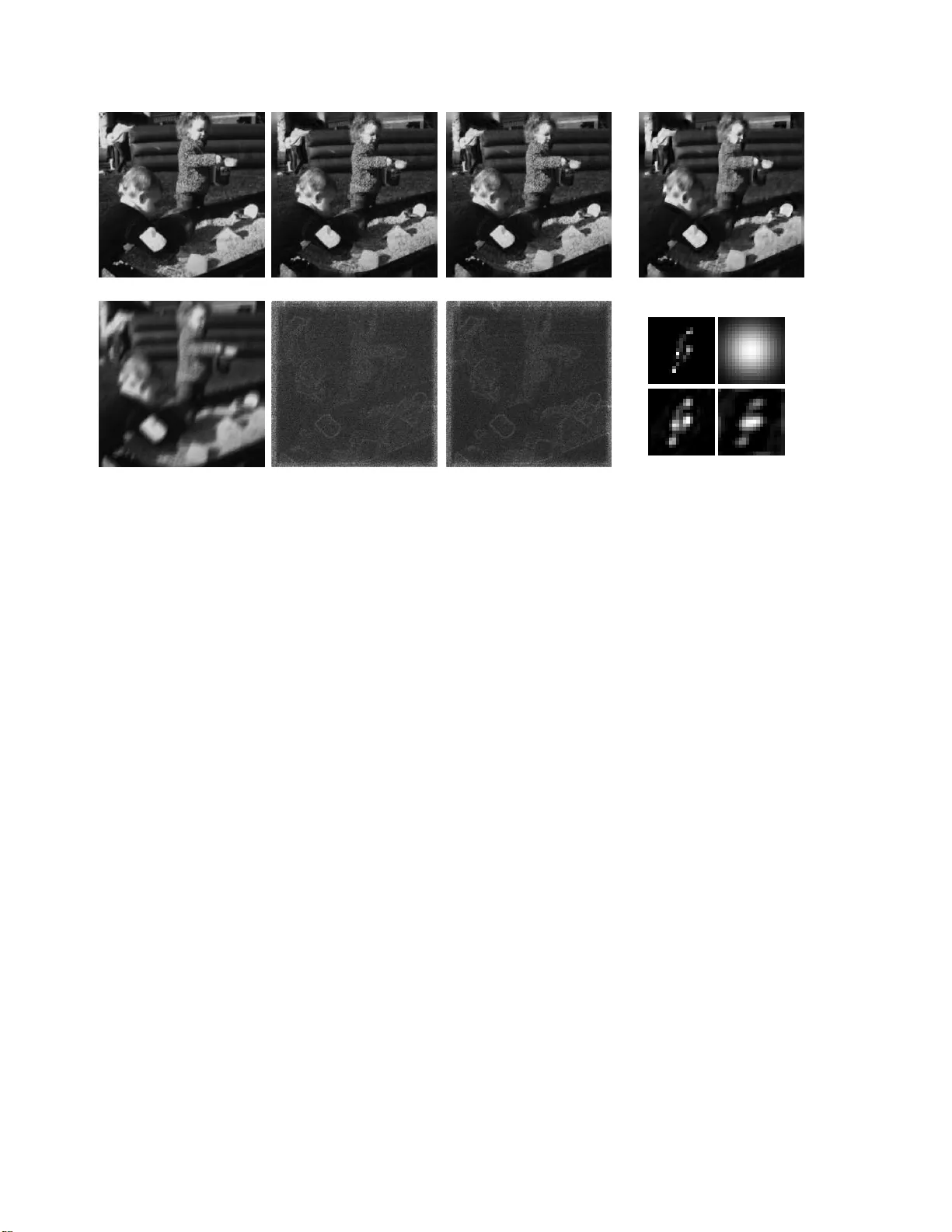
Efficient V ariational Infer ence in Large-Scale Bayesian Compressed Sensing Geor ge Papandreou 1 and Alan L. Y uille 1 , 2 1 Department of Statistics, Unive rsity of California, Los Angeles 2 Department of Brain and Cognitive Engineering, K orea Uni versity , Seoul, Korea [gpapan,yu ille]@stat .ucla.edu Abstract W e study linea r models unde r h e avy-tailed priors fr om a pr oba bilistic viewpoint. Instead of computing a single sparse most p r obab le (MAP) solu tion as in stan dar d deter- ministic appr o a ches, the foc u s in the Bayesian compressed sensing framework shifts towards cap tu ring the full poste- rior distribution on the latent variables, which allo ws q uan- tifying th e estima tio n un certainty and learnin g mo d el pa - rameters u sing maximum likelihood. The e xa ct posterior distribution under the sparse lin ear mo del is intractab le and we con centrate on v a riational Bayesian techniques to appr o ximate it. Repeatedly compu ting Gau ssian variances turns o ut to be a key r e q uisite and constitutes the main com- putation al bottleneck in ap plying va riational techniqu es in lar ge-scale p r oblems. W e leverage on the r ecently pr o- posed P erturb - and-MAP alg orithm fo r d rawing exact sam- ples fr o m Ga ussian Markov random fields (GMRF). The main technical contribution of our paper is to show tha t es- timating Gaussian variances using a relatively small n um- ber of such efficiently drawn random samp les is mu ch more effective tha n a lternative general-purpose va ria nce estima - tion techniques. By reducing the pr oblem of varian ce es- timation to standard optimization primitives, the res ulting variational alg orithms are fully sca la ble an d parallelizable, allowing Bayesian c o mputation s in extr emely la r ge-scale pr oblems with th e same memory and time com p lexity r e- quir ements as conventional point estimation techniques. W e illustrate these ideas with experiments in image deblurring. 1. Introduc tion Sparsity: Deterministic a nd Bayesian viewpoints Spar- sity has proven very f ruitful in data analysis. Ear ly metho ds such a s to tal variation (TV ) mo deling [31], wavelet thresh- olding [23], sparse coding [26], and in depend ent co mpo- nent analy sis [6] have h ad big imp act in signal and image modeling . Recen t research in compressed sensing [4, 8] has shown that h igh-dim ensional signals re presentable with fe w non-ze ro coefficients in a line ar tran sform do main are ex- actly recoverable from a small numb er of measurements throug h linear non -adaptive (ty pically random ) oper ators satisfying certain inco herence prop erties. Signal recovery in the se deter ministic models typically reduces to a conve x optimization prob lem and is scalable to prob lems with mil- lions of variables such as those arising in image analysis. The deter ministic viewpoint on sparsity has certain shortcomin gs. In real-world app lications the theor etical as- sumptions of comp ressed sensing are often vio lated. F or example, filter respo nses of natur al image s exhib it heavy- tailed m arginal histogram s but are seldom exactly zero [22]. In practical application s such as image inpa inting or deblu r- ring the measureme nt operators are fixed and do not satisfy the incoher ence proper ties. In these setups it is im possible to exactly recon struct the und erlying laten t sign al a nd it is importan t to quan tify the associated estimation unc ertainty . Along these line s, there is a growing number o f studies both in the machine learning [1, 10, 19, 36, 39] and the signal processing literature [ 5, 14] wh ich bring id eas from sparse modeling into a powerful Bayesian statistical appr oach for describing signals an d imag es. The m ost distinctive char- acteristic of Bayesian mode ling is that b eyond finding the most probable (MAP) solution it also allo ws us to repr esent the full posterio r distribution on the laten t variables, thus capturing the u ncertainty in the recovery process. From a p ractical standp oint, this Bayesian co mpressed sensing framework allows learn ing mode l p arameters and devising adaptive measu rement designs in a principled way . W e em- ploy kurtotic prior s for modelin g the heavy-tailed nature of filter responses. Beyon d sparsity , we can also capture struc- tured statist ical dependen cies b etween model variables [38] using tools fro m probab ilistic graph ical models [29], yield- ing metho ds that mor e faithfully describ e the com plex sta- tistical proper ties of real-world signals. V ariational Bayes for sparse linea r models Compu ting the exact posterior und er heavy tailed prior s is not tractable. W e thu s h av e to co ntend ou rselves with app roximate solu- tions, either of stochastic samp ling o r determin istic varia- tional type . In sampling tech niques we repr esent the poste- rior using ra ndom samples drawn by Ma rkov chain Monte- Carlo (MCMC); see [29, 30, 32, 33] for recent related work. The variational techniqu es in which we focus in this pa- per appr oximate the true posterior distribution with a pa- rameterized Gaussian wh ich allows c losed-for m computa- tions. In ference amo unts to a djusting the variational param - eters to make th e fit as tight as p ossible [41]. Mostly related to our work ar e [1, 10, 19, 36]. There exist multiple alterna- ti ve criteria to quantify the fit quality , gi v ing rise to appro x- imations such as variational bou nding [15], mean field o r ensemble learn ing, and, expectation prop agation (EP) [24] (see [ 2, 28] for discussions abou t the relations among them), as well as different iterativ e algorithms for optim izing each specific criterion. These variational criter ia inv olve some sort of integration over t he latent variables. W e should con- trast this with the Lapla ce ap proxim ation [2] which is based on a secon d-orde r T aylor expansio n around the MAP p oint estimate and is thus ina pprop riate for the o ften non-sm ooth posterior density under the sparse linear model. All variational algor ithms we study in the pap er ar e o f a double- loop nature, req uiring Gaussian variance estima- tion in the o uter loop and sparse point estimation in the in- ner loop [ 35, 3 6, 40]. The ubiq uity of the Gaussian vari- ance comp utation rou tine is n ot coinciden tal. V ariational approx imations try to cap ture un certainty in the intra ctable posterior distrib utio n a long the directions of sparsity . These are naturally enco ded in the covariance matrix of th e prox y Gaussian v ariational appro ximation. M arginal Gaussian variance computation is also requir ed in au tomatic rele- vance deter mination alg orithms for sparse Bayesian lear n- ing [20] an d relev an ce vecto r machine trainin g [39]; the methods we dev e lop could also be applied in that context. V ariance computat io n: Lanczos v s. proposed Monte- Carlo algorithm Estimating Gaussian variances is cur- rently the main c omputatio nal bo ttleneck and h inders the wider adoptio n of variational Bayesian techniques in large- scale problems with thousan ds o r millions o f variables such as th ose arising in imag e an alysis, in which explicitly stor- ing or manip ulating the fu ll covariance matrix is in gen eral infeasible. Computing variances in Gaussian Markov ran- dom fields (GMRFs) with loop s is challenging and a host of sophisticated techniques have been developed fo r this pu r- pose, which often o nly apply to restricted c lasses of mo d- els [ 21, 42]. A gen eral-pur pose v arianc e compu tation tech- nique [ 27, 34] is based on the Lanczos iterative method for solving eigenpr oblems [11] and ha s been extensively stud- ied in the variational Bayes co ntext by Seeger and Nick- isch [36 , 37]. U nless run for a proh ibitiv ely large number of iterations, th e La nczos algorithm severely under estimates the requir ed variances, to the exten t th at Lancz os is inad- equate for optimizin g criter ia like expectation p ropagatio n which are sensiti ve to gross variance estimation errors [35]. The main tec hnical contribution of our work is to dem on- strate that the sample-based Monte-Carlo Gaussian vari- ance estimato r of [3 0] p erform s markedly b etter than th e Lanczos algorithm as the key compu tational sub -routine in the v ariational learn ing co ntext. Ou r estimator builds on the efficient Perturb -and-MAP samp ling algo rithm of [30] (c.f. [29, 32]) which draws exact GM RF samples by lo- cally injecting noise to each Gaussian factor independently , followed by c omputin g the mean/mode of the per turbed GMRF by pr econditio ned conjug ate gra dients. Being u n- biased, the proposed sample estimato r does n ot suffer from the Lanczo s systematic und erestimation errors. In pr actice, a fe w samples suffice fo r captur ing the v a riances with accu- racy sufficient for e ven the more sen siti ve expectation p rop- agation algo rithm to work reliably . Mo reover , co rrelations (i.e. off-diagon al elements of covariance matrix) neede d in certain application s are easy to compu te. The advocated a pproach to Mon te-Carlo variance esti- mation for variational learn ing has several o ther advantages. It is f ully scalab le, only relying on well-studied comp uta- tional primiti ves, thus allowing Bayesian inference with the same memo ry and time complexity requireme nts as conven- tional p oint estimatio n. The p roposed a lgorithm is paral- lelizable, s ince the required Gaussian samples can be drawn indepen dently on different p rocessors. Further, we show how we can use the samples to estimate the free energy and monitor conver g ence o f the algorithm at no extra cost. 2. V ariational Bayes for sparse linear models 2.1. The s p arse linear model: Point estimation v s . Bayesian inference The fo rmulation of th e sparse linear model we consider follows the setup of [10, 36]. W e co nsider a hidden vec- tor x ∈ R N which f ollows a heavy-tailed prior d istribu- tion P ( x ) and noisy linear me asurements y ∈ R M of it are drawn with Gaussian lik elihood P ( y | x ) . Specifically: P ( x ; θ ) ∝ K Y k =1 t k ( g T k x ) , P ( y | x ; θ ) = N ( y ; Hx , σ 2 I ) , (1) where the K rows of G = [ g T 1 ; . . . ; g T K ] and the M rows o f H = [ h T 1 ; . . . ; h T M ] ar e two sets o f leng th- N linear filters, the former map ping x to the dom ain s = Gx in which it e x- hibits sp arse respon ses and the latter captur ing the Gaussian measuremen t proce ss 1 . The sparsity indu cing potentials are d enoted b y t k ( s k ) . The Laplacian t k ( s k ) = e − τ k | s k | , s k = g T k x , is a widely used form for them. In some appli- cations a subset of the mode l’ s aspects ( H , σ 2 , G ) can b e unknown and dep endent o n a par ameter vector θ ; e.g ., in 1 N ( x ; µ , Σ ) = | 2 π Σ | − 1 / 2 exp  − 1 2 ( x − µ ) T Σ − 1 ( x − µ )  is the multi varia te Gaussian densit y on x with mean µ and cov arianc e Σ . blind image decon volution θ typically is the unknown b lur- ring kernel k which determ ines the measurement matrix H . By Baye s’ ru le, the posterior distribution of the latent variables x given y h as the non-Gaussian density P ( x | y ) = Z − 1 ( θ ) P ( y | x ) K Y k =1 t k ( s k ) , where (2) Z ( θ ) , P ( y ; θ ) = Z P ( y | x ) K Y k =1 t k ( s k ) d x (3 ) is the e vidence/ partition function . Point estimatio n corresp onding to standard comp ressed sensing amo unts to finding the posterior MAP co nfiguratio n ˆ x MAP , argma x x log P ( x | y ) , leadin g to minimization of φ MAP ( x ) = σ − 2 k y − Hx k 2 − 2 K X k =1 log t k ( s k ) . (4) Point estimation th us reduces to a stand ard optimization problem and a host of moder n techn iques hav e b een de- veloped f or solving it, scalable to large-scale application s. Howe ver, since it ign ores the p artition fu nction, po int es- timation n either p rovides infor mation abo ut the estimation uncertainty nor allo ws parameter estimation. In the Bayesian fram ew o rk we tr y to overcome these shortcomin gs b y captu ring the full po sterior distribution. Since it is intractab le to manipu late it d irectly , we consid er variational approx imations of Gaussian form Q ( x | y ) ∝ P ( y | x ) e β T s − 1 2 s T Γ − 1 s = N ( x ; ˆ x Q , A − 1 ) , with ˆ x Q = A − 1 b , A = σ − 2 H T H + G T Γ − 1 G , Γ = diag( γ ) , and b = σ − 2 H T y + G T β . ( 5) The implied form for the variational evidence is Z Q ( θ ) , Q ( y ; θ ) = Z P ( y | x ) e β T s − 1 2 s T Γ − 1 s d x . (6) Our task in variational learnin g is to adjust th e set of varia- tional par ameters ξ = ( β , γ ) so as to improve the fit of the approx imating Gaussian to the true posterior distribution. W e will mostly be f ocusing o n log-concave sparsity in- ducing potentials t k ( · ) – i.e., log t k ( · ) is concave – suc h as the Laplacian . This g uarantees that the p osterior P ( x | y ) is also lo g-concave in x , and thus p oint estimatio n in Eq. (4) is a conve x optimization problem. Log -concavity also implies that P ( x | y ) is unimod al and justifies approxim ating it with a Gaussian Q ( x | y ) in Eq . (5). 2.2. V ariational bo unding V ariational boun ding [10, 15, 28, 36] is app licable to sparsity-indu cing potentials of super-Gaussian fo rm. The family of even super-Gaussian p otentials is quite r ich and superset of the family of mixtures of zero- mean Gaussians; it in cludes the Laplacian and the Student as memb ers [2 8]. Super-Gaussian p otentials ha ve a u seful dual representation t k ( s k ) = sup γ k > 0 e − s 2 k / (2 γ k ) − h k ( γ k ) / 2 , with (7) h k ( γ k ) , sup s k − s 2 k /γ k − 2 log t k ( s k ) (8) V ariational b ound ing amounts to replacin g the potentials t k ( s k ) in Eq. ( 2) with these b ound s an d tuning the varia- tional parameters γ ( β is fixed to zero in this case) so as the variational e viden ce lo wer boun ds as tightly as possible the exact evidence Z ≥ Z Q . T his leads to the variational free energy minimization proble m (see [ 36] fo r the d eriv ation ) inf γ ≻ 0 φ Q ( γ ) , where φ Q ( γ ) = lo g | A | + h ( γ ) + inf x R ( x , γ ) , (9) with h ( γ ) , P K k =1 h k ( γ k ) and R ( x , γ ) , σ − 2 k y − Hx k 2 + s T Γ − 1 s . The A and b are giv en in Eq. ( 5); note that A is a function of γ . The log -determin ant term in Eq. (9) is what makes Bayesian variational inferen ce mo re in teresting a nd at the same time co mputation ally more de manding tha n p oint e s- timation. Indeed, using Eq. (7), we ca n r e-write th e o b- jectiv e fun ction fo r MAP estimation (4) as φ MAP ( x ) = inf γ ≻ 0 h ( γ ) + R ( x , γ ) , showing that φ MAP and φ Q only differ in the log | A | ter m, wh ich endows variational in fer- ence with the ability to cap ture th e effect o f the partition function . The d ifficulty lies in the fact that the elements of the vector γ ar e interleaved in log | A | . Following [28, 36], we can decouple the prob lem by exploiting the concavity of log | A | as a fun ction o f γ − 1 , ( γ − 1 1 , . . . , γ − 1 K ) . Fenchel du - ality then yields th e uppe r b ound log | A | ≤ z T γ − 1 − g ∗ ( z ) , z ≻ 0 . F or giv en γ the bo und becomes tight for z = ∇ γ − 1 log | A | = diag ( GA − 1 G T ) , wh ich can b e iden tified as the vector of marginal variances z k = V ar Q ( s k | y ) along the direc tions s k = g T k x un der the variational posterior Q ( x | y ) with the c urrent guess for the parameters γ . This approa ch naturally sug gests a double-loo p algo- rithm, glo bally convergent when the poten tials t k are lo g- concave [28, 36]. In the o uter loo p , we comp ute the vector of m arginal variances z so as to tigh ten the upp er bou nd to log | A | , given the curr ent v alu e of γ . In the inner loo p , instead of φ Q in Eq. (9) we minim ize w . r .t. x and γ the upper bound giv en the ne wly comp uted z ¯ φ Q ( x , γ ; z ) = z T γ − 1 + h ( γ ) + R ( x , γ ) = σ − 2 k y − Hx k 2 + K X k =1  s 2 k + z k γ k + h k ( γ k )  . (10) W e can minim ize this expression explicitly w .r .t. γ by not- ing that it is decou pled in the γ k and recalling fro m (7) that − 2 log t k ( s k ) = inf γ k > 0 s 2 k /γ k + h k ( γ k ) . This leaves us with a minimization problem w . r .t. x alone ¯ φ Q ( x ; z ) = inf γ ≻ 0 ¯ φ Q ( x , γ ; z ) = = σ − 2 k y − H x k 2 − 2 K X k =1 log t k  ( s 2 k + z k ) 1 / 2  . (11) This is just a smoothed version of the MAP point estima- tion prob lem (4), also con vex when t k are log -concave, which we minimize in the course of the inner loo p with standard quasi-Newton methods [3] to obtain the varia- tional mean ˆ x . After completio n of the in ner loop, we r e- cover th e m inimizing values fo r the variational parame ters γ − 1 k = − 2 d log t k ( √ v ) dv    v = ˆ s 2 k + z k , with wh ich we update the vector of marginal v a riances z in the subseq uent outer loop iteration [36]. 2.3. Mean field and expe ctation propagation Bounding is no t the only way to construct variational approx imations to the intractab le po sterior distrib ution P ( x | y ) . Th e mean field ( or en semble learnin g) app roach amounts to assum ing a simplified par ametric fo rm Q for the posterior d istribution and ad justing th e co rrespond ing v ari- ational parameter s ξ so as to minimize the KL-divergence D K L ( Q || P ) between Q an d P [1] . See [1 8] for a recent application of the mean field appro ximation to the pr oblem of image dec on volution, wh ere it is shown that the mea n field up dates reduce to p oint estimatio n and variance com- putation p rimitives, exactly as in the variational bou nding approx imation discussed in detail in Sec. 2.2. Expectation pro pagation ( EP) is yet anoth er p owerful variational approxim ation criterion , in which the variational parameters of the a pprox imating distribution Q are adjusted so as expectation s under Q and the tru e posterior P ( x | y ) are matched [2 4]. Ther e are various iterativ e seq uential message p assing-like algor ithms fo r o ptimizing th e EP cri- terion. App lying E P to large-scale problems in which ou r paper focu ses is challen ging. W e w ill employ th e parallel update alg orithm of [40], b ut o ur me thods are also appli- cable to the recently pr oposed prov ably con vergent doub le- loop algo rithm of [35]. Onc e mor e, variance estimatio n in the outer loop is the computatio nal bottlene ck; see [35, 40]. 3. Monte-Carlo posterior variance estimation As highlighted in Sec. 2, r epeatedly co mputing poste- rior Gaussian variances turns out to be a ke y computational routine in all variational app roximation s of the sparse lin- ear m odel. W ith ref erence to Eq. (5), o ur goal is to c om- pute certain elemen ts of the covariance matr ix Σ , A − 1 or m arginal variances z k = V ar Q ( s k | y ) along certain pro- jections s k = g T k x un der the variational posterior Q ( x | y ) . Note th at Σ is a fully den se N × N matrix. Thu s for large- scale mo dels c omprising N ≈ 10 6 variables it is im possible to compute or store the full Σ explicitly . 3.1. Lanczos varianc e estimation So far, the main ca ndidate for variance estimation in th e context of large- scale variational Bayes h as been the L anc- zos iterative m ethod [36, 37]. As the iter ation p rogresses, the Lanc zos algorithm builds a monoton ically incr easing estimate for the variances [11]. It can r ev eal in relatively few iterations the rou gh structure and relati ve magn itude of variances, but re quires a very la rge n umber of iterations to accurately app roximate their absolu te values. Since it scales badly with th e numbe r of iterations N L (its c omplexity is O ( N 2 L ) in time and O ( N L ) in memo ry due to a r equired reortho gonalization step), it is only prac tical to run Lanczo s for a r elativ ely small nu mber of iteration s, yie lding gro ss undere stimates for the variances. In practice, variational boun ding has proven relativ ely robust to the Lan czos cru de variance estimates [36, 37], while expectatio n prop agation comp letely fails [ 35]. Th is starkly contrasting qualitative be havior in the two cases can be explained as fo llows: I n the presen ce of Lanc zos vari- ance underestimation er rors, the expression (10) remains an upper boun d of (9 ), albeit no t tigh t any more . Moreover , the variational o ptimization p roblem ( 11) gr acefully degrad es to the poin t estimation problem (4) when 0 ≤ ˆ z k ≪ z k . In other words, despite the variance errors the algorith m does not collapse, althoug h it effecti vely ends up solving a mo d- ified inferenc e prob lem ra ther th an th e one that it was sup - posed to solve. In co ntrast, expec tation p ropag ation works by mom ent ma tching and the gross variance estimation er- rors make iterati ve EP algorith ms hopelessly break do wn . 3.2. Efficient Monte-Carlo variance estimation with Perturb-and-MAP sampling W e propo se estimating variances using a sampling -based Monte-Carlo technique, le verag ing on the efficient Perturb- and-MAP GMRF samplin g algorithm of [30]. Although [30] has already sug gested this possibility , it h as not ex- plored its effecti veness in the v ar iational Bayesian context. The alg orithm of [30] reduces GMRF samp ling in to a GMRF mean estimation pro blem. In our n otation, an exact Gaussian sample ˜ x ∼ N ( 0 , A − 1 ) , with A = σ − 2 H T H + G T Γ − 1 G , can be drawn by solving the linear s ystem A ˜ x = σ − 2 H T ˜ y + G T ˜ β . (12) The lo cal perturbation s ˜ y ∼ N ( 0 , σ 2 I ) and ˜ β ∼ N ( 0 , Γ − 1 ) a re tri vial to sample since Γ is diagonal. W e ef- ficiently solve the linear system (12) usin g precon ditioned conjuga te g radients (PCG) [1 1], employing filtering ro u- tines for fast e valuation of matrix-vector products Ax , thus av oid ing the costly Cholesky factor ization step typically as- sociated with Gaussian simulation. In contrast to Lanczo s, the memory foo tprint of PCG is small as o nly 4 length - N vectors need to be stored, while multip le sam ples can be trivially drawn in par allel (using, e.g ., parfor in Mat- lab). A lso no te that, unlike conjug ate gradients, em ploying precon ditioning within Lanczos variance estimation is dif- ficult [34] and seldom used in practice. Having drawn N s Gaussian samples as de scribed, we employ the standard sample-based cov arianc e estimators ˆ Σ = 1 N s N s X i =1 ˜ x i ˜ x T i , ˆ z k = 1 N s N s X i =1 ˜ s 2 k,i , (1 3) with ˜ s k,i , g T k ˜ x i . The variance estimates ma rginally fol- low scaled chi-square distributions with N s degrees of free- dom ˆ z k ∼ z k N s χ 2 ( N s ) . This implies tha t E { ˆ z k } = z k , i.e., this estimator is u nbiased, unlike th e Lan czos one. I ts rela- ti ve error is r = ∆( ˆ z k ) /z k = p V ar( ˆ z k ) /z k = p 2 / N s , in- depend ent from the prob lem size N . Th e error drops quite slowly with the number of samp les ( N s = 2 /r 2 samples are require d to reach a desired r elativ e error r ), but vari- ance estimates sufficiently accurate for even the more sen - siti ve expectation pro pagation alg orithm to work reliably can be obtaine d after ab out 2 0 samples (which translates to r ≈ 32% ). One ca n show that z k ≤ γ − 1 k [36], a co n- sequence of the fact that measuremen ts always red uce the uncertainty in Gaussian models. T o enf orce this im portant structural constraint, we use in place of (13) the clipped esti- mator ¯ z k = min( ˆ z k , γ − 1 k ) which beh av es considerably bet- ter in practice while still being (asymptotically ) unb iased. T o illustrate the efficiency of the pro posed Monte- Carlo variance estimator in the con text of variational Baye sian in- ference, we co mpare in Fig . 1 the m arginal variances ob- tained by ou r sample-based estimator with th at of Lan czos. The system matr ix A for this particular example is the o ne of the last iteration of th e d ouble-lo op variational bou nd- ing a lgorithm o f Sec. 2.2 applied to a small- scale 4 8 × 73 deblurr ing prob lem for which it is fea sible to compu te the exact m arginal variances z k . W e use the clipped version ¯ z k of our estimato r with N s = 20 samples, each drawn by solving the linear sy stem (12 ) with 2 0 PCG iterations as de- tailed in Sec. 4. Lanczos was run for N L = 300 iteration s, so as the runtime for the two algorithms to be the same. W e see that the pro posed samp le-based variance estimator per- forms marked ly better th an Lan czos, wh ich gr ossly under- estimates the true ma rginal variances. Note that fo r large- scale problems the performance gap will be e ven more pro- nounc ed: as w e showed earlier, the relativ e estimation accu- racy r of the samp le-based estimato r is independ ent o f the latent space dimension ality N , while the relative accur acy of Lanczos further deteriorates for large N [36, Fig. 6]. 0 2 4 6 8 x 10 −3 0 2 4 6 8 x 10 −3 z k ˆ z k SAMPLE LANCZOS EXACT Figure 1. S catter-plot of exac t z k vs. estimated ˆ z k marginal vari- ances for a small-scale deblurring problem. W e compare the the proposed sample-based Monte-Carlo estimator with Lanczos. 3.3. Monte-Carlo free e nergy es timation T o monitor conv ergence of th e free en ergy (9) an d fo r debugging p urposes, it is desirable to estimate log | A | dur- ing the course of the algo rithm. Note that this step is not a requisite for th e variational algorithm to yield estimates f or x or estimate the model parameters θ . By coercing info rmation from th e sam ples ˜ x ∼ N ( 0 , A − 1 ) drawn f or variance estimation, we can reli- ably estimate log | A | at no extra co st, p rovided that we can analy tically com pute log | P | fo r so me matrix P that approx imates A well, typically th e p recond itioner em - ployed by PCG for solving (12). T o see this, note that E  exp  0 . 5 ˜ x T ( A − P ) ˜ x  = | A | / | P | , which sug gests the Monte-Carlo estimator log | A | ≈ log | P | − log N s + log N s X i =1 0 . 5 ˜ x T i ( A − P ) ˜ x i ! . (14) A special case of this with P = I has been proposed before [7], but for the lar g e-scale problems we c onsider here using a good ref erence P ≈ A is crucial for the estimator (1 4) to exhibit lo w variance and thus be useful in practice. 4. Applications to image decon volution Our ma in motiv atio n f or this work is so lving in verse problem s in imag e an alysis and low-le vel vision such as im- age deblurring, inpain ting, and tomographic re construction . These g iv e rise to large-scale in ference pro blems in volving millions of variables. W e report expe rimental results on im- age deconv olutio n. Our software builds on the glm-ie Matlab too lbox [2 5] d esigned for variational infer ence un- der the variational b oundin g [36] an d expe ctation propa ga- tion [40 ] criteria, which we ha ve extended to include imple- mentations o f th e propo sed algorithms; our extensions will be integrated in future releases of glm-ie . In im age d eblurrin g [1 2, 13], our goal is to r ecover the sharp im age x from its blur red version y . W e assume a spatially homo geneou s degradatio n, ty pically due to cam- era or subject motion , captu red by the m easurement pr ocess y = Hx , k ∗ x . In the no n-blind variant o f the p rob- lem, t he con volution blu r kernel k is consider ed kn own (the problem is classically known as imag e restoration) , while in the mor e challeng ing blind variant ou r goal is to rec over both the sharp image and the unknown blurr ing k e rnel. Blind image dec o n volutio n In the blind dec onv olutio n case, the blurring kernel i s considered as parameter, θ = k , which we recover by maximum (penalized ) likelihood. It is cr ucial to determ ine k by first integrating out the laten t variables x and th en maximizing the margin al likeliho od argmax k P ( y ; k ) , in stead o f maximizing the joint likeli- hood argmax k (max x P ( x , y ; k )) [9, 17]. Un der the varia- tional ap proxim ation, we use Q ( y ; k ) from (6) in place of P ( y ; k ) . Following [10, 18], we carry out the optimization iterativ ely using e x pectation- maximization (EM). In the E- step , giv en the cu rrent e stimate k t for th e blurring kernel, we perf orm variational Bayesian inf erence as described in Sec. 2. In th e M-step of th e t -th iter- ation, we maximize w .r .t. k th e expe cted complete log- likelihood E k t { log Q ( x , y ; k ) } , with expectations taken w . r .t. Q ( x | y ; k t ) . Th e updated kernel k t +1 is obtain ed by minimizing w .r .t. k (see [1 8] for the deri vation) E k t  1 2 k y − Hx k 2  = 1 2 tr  ( H T H )( A − 1 + ˆ x ˆ x T )  − y T H ˆ x + (cons t) = 1 2 k T R xx k − r T xy k + (cons t) , (15) which is a quad ratic progr am in k ; see [18] for the for mu- las f or r xy and R xx . The entries in r xy accumulate cross- correlation s between ˆ x and y ; we u se the variational mea n ˆ x of (11) for co mputing them . The entries in R xx capture second-o rder inf ormation for x under Q ( x | y ; k t ) ; we es- timate th em efficiently by drawing a small num ber of sam- ples ( 1 o r 2 suffice) fro m N ( 0 , A − 1 ) , exactly a s in Sec. 3.2. Note that [18 ] estimates R xx by making the simplif ying as- sumption that A is d iagonal, which could potentially lead to a poo r appro ximation. W e add to (15) an extra L 1 penalty term λ 1 k k k L 1 so as to fa vor sparse kernels. It is im portant to no te that wh ile the M-step u pdate for k in (15) is a conve x optimization problem, the overall log- likelihood objective − log Q ( y ; k ) is not convex in k . This means that the EM algorithm can ge t stuck to local min- ima. V arious techn iques have b een developed to mitigate this fu ndamenta l problem, suc h as coar se-to-fine kernel re- covery , gradien t d omain proce ssing, o r regularizatio n of the result after each kernel u pdate with (15) – see [ 9, 17]. W e have n ot yet incorporated these heur istics into our blind de- conv olutio n implem entation, and thus ou r software may still giv e un satisfactory re sults wh en the spatial supp ort o f the unknown blurring k e rnel is large. Efficient circulant preconditioning Our sample-based variance estimator described in S ec. 3.2 requires repeatedly drawing samples ˜ x . For each of the samp les we solve by PCG a lin ear system of the fo rm A ˜ x = ˜ c , where ˜ c is the random ly pertu rbed right hand side in Eq. (12). The system matrix A = σ − 2 H T H + G T Γ − 1 G arising in imag e deb lurring is typically po orly con ditioned, slow- ing th e co n vergence of plain conjugate g radients. The key to d esigning an effecti ve pr econditio ner for A is to note that A wou ld be a stationar y oper ator if Γ = ¯ γ I , i.e. , the varia- tional p arameters γ k were homo geneou s. Following [1 6], we select as p recond itioner the stationary approxim ation of th e sy stem matrix , P = σ − 2 H T H + ¯ γ − 1 G T G , with ¯ γ − 1 , (1 /K ) P K k =1 γ − 1 k . One can prove that P is the stationary matrix nearest to A in th e Frob enius n orm, i.e. P = argmin X ∈C k X − A k , where C is the set of station- ary (b lock-circu lant with circulan t blocks) matrices [16]. Thanks to its stationarity , P is diagon alized in the Fourier domain; b y em ploying the 2 -D DFT , we can c ompute very efficiently expressions of the for m P − 1 x requir ed by PCG [12]. Moreover, log | P | is also read ily com putable in the Fourier domain, allowing us to use the efficient free energy estimator ( 14) fo r mon itoring conver gence. Note tha t the applicability of this p recond itioner extends beyond our vari- ance estimation setup; e.g. it could be employed in conjunc- tion with the MCMC-based deblurrin g algor ithm of [33]. Circulant p recond itioning with P d ramatically acceler- ates co n vergence of conjug ate gr adients. W e plot in Fig. 2 the residual in the course of conjugate grad ient iteration for a typical system matrix A ar ising in deblurrin g a 190 × 289 image un der the variational bo unding appro ximation. W ith circulant precon ditioning (PCG) we attain within o nly 1 0 iterations the sam e level o f accuracy that is reached af- ter 100 iterations of un precon ditioned co njugate g radients (CG). This substantial im provement in the convergence rate more than compensates the roughly 60% time overhead per iteration of PCG relativ e to CG (resp ectiv e ly , 80 vs. 50 m sec per iteration on this pro blem). W e ar e not aware of any work that similarly exploits the benefits of precondition ing in the context of Lanczos v aria nce estimation. Image deblurring results W e h av e carr ied ou t prelim i- nary image deblurring exper iments using the da taset of [17] which contains images degraded by real blur due to camera motion, a s well as their shar p versions shot with th e cam- era still. W e assum e a total-variation p rior, which implies simple first-order finite difference filters as rows of G a nd Laplacian spar sity in ducing pote ntials t k ( s k ) = e − τ k | s k | . 0 20 40 60 80 100 120 10 −15 10 −10 10 −5 10 0 10 5 10 10 CG PCG Figure 2. Conjugate gradients residual norm as function of itera- tion count; No (CG) vs. circulant (PCG) preconditione r . W e fix τ k = 15 which rou ghly matches the image deriva- ti ve scale for typical im ages with values b etween 0 an d 1. W e set the noise variance to σ 2 = 10 − 5 . W e em ploy the d ouble- loop a lgorithms describ ed in Sec. 2 fo r both th e variational bound ing (VB) and expec- tation propagatio n (E P). W e use 20 sam ples f or v ariance estimation, and allo w 20 PCG iterations for solving each of the linear systems (12). W e s how the deblu rred images fro m both the VB and EP algo rithms in Fig. 3 for both the n on- blind and blind scenaria. Note th at E P c ompletely break s down if we u se the L anczos variance estimator, while it re - liably works under our sample-based v ar iance estimator . 5. Discussion W e have shown th at marginal variances require d by v ari- ational Bayesian algo rithms can be effectiv ely estimated using r andom samplin g. This allows app lying variational Bayesian inf erence to large-scale pro blems, essentially at the same co st a s p oint estimation. The propo sed variance estimator can be thought as a stochastic sub-ro utine in the otherwise deterministic v ariational framework. Interestingly , efficient Pertu rb-and -MAP random sam- pling turns o ut to be a key componen t in both the pro posed approa ch to variational inference and recen t MCMC tech- niques [29, 30, 32, 33]. Systematically comparin g these two alternative Bayesian inference alternatives in lar g e-scale ap- plications arises as an interesting topic for future work. Acknowledgments This work was suppo rted by the U.S. Office of Nav al Re- search und er the MURI g rant N000 1410 10933 and by the K o rean Ministry of Educatio n, Science, a nd T ech nology , under the National Research Foundation WCU p rogram R31-100 08. W e thank S. Lefkimmiatis fo r sug gesting the circulant precond itioner of Sec. 4, M . Seeger for his feed- back on an earlier version of the paper, an d H. Nickisch for making the glm-ie toolbox publicly av ailable. Refer ences [1] H. Attias. Inde pendent factor analysis. Neur . Comp. , 11:803 – 851, 1999. [2] C. Bishop. P attern Recognition and Machine Learning . Springer , 2006. [3] R. Byrd, P . Lu, and J. Noced al. A limited memory algorithm for b ound co nstrained optimization. SIAM J. Sci. and Statist. Comp. , 16(5):119 0–1208, 1995. [4] E. Candes and T . T ao. Decoding by linear programming. IEEE T rans. Inf. Theory , 51(12):4203– 4215, Dec. 2005. [5] V . Ce vher , P . Indy k, L. Carin, and R. Baraniuk. Sparse sign al recov ery and acquisition with graphical models. IEEE Signal Pr ocess. Mag. , 27(6):92–103 , Nov . 2010. [6] P . Comon. Independent component analysis, a n ew concept? Signal Proce ssing , 36(3):287–3 14, 1994. [7] N. Cressie, O. Perrin, and C. T homas-Agnan . Likelihood - based estimation for Gaussian MRFs. Stat. Meth. , 2(1 ):1–16, 2005. [8] D. L. Donoho. Compressed sensing. IEEE T rans. Inf. The- ory , 52(4):1289– 1306, Apr . 2006. [9] R. Fergus, B. Singh, A. Hertzmann , S. Ro weis, and W . Free- man. Remov ing camera shake from a single photograph. Pr oc. SIGGRA PH , 25(3):78 7–794, 2006. [10] M. Girolami. A variational method for learning sparse and ov ercomplete representations. Neur . Comp. , 13:2517–2 532, 2001. [11] G. Golub and C. V an Loan. Matrix Computations . John Hopkins Press, 1996. [12] P . Hansen, J. Nagy , and D. O’Leary . Deblurring images : matrices, spectra, and filtering . SIAM, 2006. [13] A. Jain. Fundamentals of digital imag e pr ocessing . P rentice Hall, 1989. [14] S. Ji, Y . Xue, and L. Carin. Bayesian compressiv e sensing. IEEE T rans. Signal Pr ocess. , 56(6):2346– 2356, June 2008. [15] M. Jordan, J. G hahramani, T . Jaakkola, and L. S aul. An in- troduction to va riational methods for graphical models. Ma- chine L earning , 37:183–2 33, 1999. [16] S. Lefkimmiatis, A. Bourquard, and M. Unser . Hessian- based norm regularization for image restoration with biomedical applications. IEEE T rans. Image Proces s. , 2012 . to appear . [17] A. Levin , Y . W eiss, F . Dura nd, an d W . Freeman. Understand- ing and ev aluating blind decon volution algorithms. In P roc. CVPR , pages 1964–1 971, 2009. [18] A. Le vin, Y . W eiss, F . Durand, and W . Freeman. E fficient marginal li kelihoo d optimization in blind decon volution. In Pr oc. CV PR , pages 2657– 2664, 2011. [19] M. Le wicki and T . Sejno wski. L earning o vercomplete repre- sentations. Neur . Comp. , 12:337 –365, 2000. [20] D. MacKay . Bayesian interpo lation. Neur . Comp. , 4(3):415– 447, 1992. [21] D. Maliouto v , J. Johnson, M. Choi, and A. Willsky . Low- rank variance approximation in GMRF models: Single and multiscale approaches. IEEE T rans. Signal Proc ess. , 56(10):4621 –4634, Oct. 2008. (a) sharp (c) VB mean (PSNR=31.93dB) (e) EP mean (PSNR=31.85dB) (g) blind VB mean (PSNR=27.54dB) (b) blurre d (PSNR=22.57dB) (d) VB stdev (f) EP stde v (h) kernel e volution Figure 3. Image deblurring experiment with the proposed algorithms. (a) Sharp 255 × 25 5 image. (b) R eal blurred image. Posterior mean and pointwise estimation uncertainty for non-blind image deblurring under the v ariati onal bound ing (c, d) and expectation propagation (e, f) criteria. (g) Blind image deblurring with variationa l bounding. (h) clockwise from upper left, ground-truth 19 × 19 blurring kernel, initialization, and estimated kernels after the fi rst and the final tenth EM iteration. The model estimates t he image v al ues in an extended 273 × 273 domain, but we only tak e the central 255 × 255 area into account when calculating the PSNR. [22] S. Mallat. A theory for multiresolution signal decomposi- tion: The wa velet transform. I E EE T rans. P AMI , 11(7 ):674– 693, 1989. [23] S. Mallat. A W avelet T our of Signal Processin g . Acad. Press, 2 edition, 1999. [24] T . Minka. Expectation propagation for approxima te bay esian inference. In Pr oc. U A I , 2001. [25] H. Nickisch. The generalised line ar models in- ference and esti mation toolbox (glm-ie v . 1.3). http://mloss. org/software/ view/269 . [26] B. Olshausen and D. Fi eld. Emergence of simple-cell re- cepti ve field properties by learning a sparse code for natural images. Natur e , 381:607–6 09, 1996. [27] C. Paige and M. S aunders. L SQR: An al gorithm for sparse linear equations and sparse least squares. ACM Tr ans. on Math. Soft. , 8(1):43–71, 1982. [28] J. Palmer , D. W i pf, K. Kreutz-Delgado, and B. Rao. V aria- tional EM algorithms for non-gaussian latent variable mod- els. In Pr oc. NIPS , 2005. [29] G. Papandreo u, P . Maragos, and A. K okaram. Image inpaint- ing with a wav elet domain hidden Marko v tree model. In Pr oc. IC A SSP , pages 773–7 76, 2008. [30] G. Papand reou and A. Y uille. Gaussian sampling by local perturbations. In Pr oc. NIPS , 2010. [31] L. Rudin, S. Osher , and E. Fatemi. Nonlinear total va riation based noise remov al algorithms. P hysica D , 60:259–268 , 1992. [32] U. Schmidt, Q. Gao, and S. Roth. A generativ e perspectiv e on MRFs in lo w-level vision. In Pro c. CVPR , 2010. [33] U. Schmidt, K. Schelten, and S. Roth. Bayesian deblur- ring with integrated noise estimation. In Proc. CVPR , pages 2625–2 632, 2011. [34] M. Schneider and A. Willsk y . Krylov subspace estimation. SIAM J. Sci. Comp. , 22(5):1840–1 864, 2001. [35] M. Seeger and H. Nickisch. Fast con verg ent algorithms for expec tation propagation approximate bayesian inference. In Pr oc. A I ST ATS , 2011. [36] M. Seeger and H. Nickisch. Large scale bayesian inference and experimental design for sparse linear models. SIAM J . Imaging Sci. , 4(1):166–1 99, 2011. [37] M. Seeger , H. Ni ckisch, R . Pohmann, and B. Sch ¨ olkop f. Bayesian experimental design of magnetic resonance i mag- ing sequences . In Pro c. NIPS , pages 1441–1448, 2008. [38] E. P . Simoncelli. Statistical modeling of photog raphic im- ages. In A. Bovik, editor , Handboo k of V ideo and Imag e Pr ocessing , chapter 4.7. Academic Press, 2 edition, 2005. [39] M. Tip ping. S parse Bayesian learning and the rele vance vec- tor machine. J. of Mach. Learn. Res. , 1:211–244, 2001. [40] M. van Gerven, B. Cseke, F . de Lange, and T . Heskes. Effi- cient B ayesian multiv ariate fMRI analysis using a sparsify- ing spatio-temporal prior . Neur oImage , 50:150–16 1, 2010. [41] M. W ainwright and M. Jordan. Graphical models, exponen- tial fa milies, and v ariational inference. F ound. and T r ends in Mach ine Learning , 1(1-2):1– 305, 2008. [42] Y . W eiss and W . Freeman. Correctness of belief propagation in Gaussian graphical models of arbitrary topology . Neur . Comp. , 13(10):21 73–2200 , 2001.