Accelerated, Parallel and Proximal Coordinate Descent

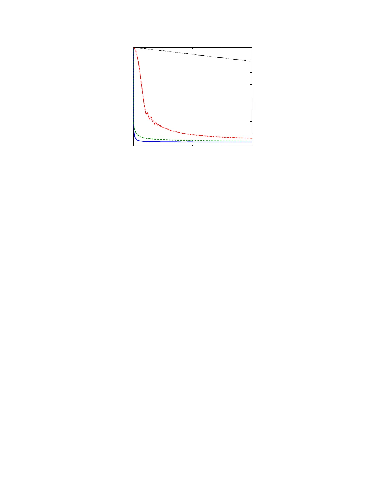
Accelerated, P arallel and Pro ximal Co ordinate Descen t Olivier F erco q ∗ P eter Rich t´ arik † Decem b er 19, 2013 (up dated: F ebruary 2014) Abstract W e propose a new sto chastic coordinate descen t method for minimizing the sum of conv ex functions eac h of whic h dep ends on a small n um b er of co ordinates only . Our method (APPR OX) is sim ultaneously Accelerated, P arallel and PR OXimal; this is the first time suc h a metho d is proposed. In the sp ecial case when the num b er of pro cessors is equal to the num ber of co ordinates, the metho d conv erges at the rate 2 ¯ ω ¯ LR 2 / ( k + 1) 2 , where k is the iteration coun ter, ¯ ω is an aver age degree of separabilit y of the loss function, ¯ L is the aver age of Lipschitz constan ts asso ciated with the co ordinates and individual functions in the sum, and R is the distance of the initial point from the minimizer. W e show that the method can b e implemen ted without the need to p erform full-dimensional vector operations, whic h is the ma jor b ottlenec k of accelerated co ordinate descent. The fact that the metho d dep ends on the av erage degree of separability , and not on the maxim um degree of separability , can b e attributed to the use of new safe large stepsizes, leading to improv ed exp ected separable ov erapproximation (ESO). These are of indep enden t interest and can b e utilized in all existing parallel sto c hastic co ordinate descent algorithms based on the concept of ESO. 1 In tro duction Dev elopments in computing tec hnology and ubiquit y of digital devices resulted in an increased in terest in solving optimization problems of extremely big sizes. Applications can b e found in all areas of h uman endeav or where data is a v ailable, including the internet, machine learning, data science and scien tific computing. The size of these problems is so large that it is necessary to decomp ose the problem in to smaller, more manageable, pieces. T raditional approaches, where it is p ossible to rely on full-vector op erations in the design of an iterativ e scheme, must b e revisited. Co ordinate descent metho ds [12, 17] app ear as a very p opular class of algorithms for such problems as they can break do wn the problem into smaller pieces, and can tak e adv an tage of sparsit y patterns in the data. With big data problems it is necessary to design algorithms able to utilize mo dern parallel computing architectures. This resulted in an in terest in parallel [16, 21, 3, 15] and distributed [14] co ordinate descent metho ds. ∗ Sc ho ol of Mathematics, The Univ ersity of Edinburgh, United Kingdom (e-mail: olivier.ferco q@ed.ac.uk) † Sc ho ol of Mathematics, The Universit y of Edin burgh, United Kingdom (e-mail: peter.rich tarik@ed.ac.uk) The w ork of b oth authors w as supported by the EPSRC gran t EP/I017127/1 (Mathematics for V ast Digital Resources) and by the Cen tre for Numerical Algorithms and In telligent Soft ware (funded by EPSR C grant EP/G036136/1 and the Scottish F unding Council). The w ork of P .R. was also supp orted b y EPSRC grant EP/K02325X/1 (Accelerated Co ordinate Descent Metho ds for Big Data Problems) and b y the Simons Institute for the Theory of Computing at UC Berk eley . 1 In this work we fo cus on the solution of conv ex optimization problems with a huge num b er of v ariables of the form min x ∈ R N f ( x ) + ψ ( x ) . (1) Here x = ( x (1) , . . . , x ( n ) ) ∈ R N is a decision vector comp osed of n blo cks, with x ( i ) ∈ R N i , f ( x ) = P m j =1 f j ( x ) , (2) where f j are smo oth conv ex functions, and ψ is a blo ck separable regularizer (e.g., L 1 norm). In this work we make the follo wing three main contributions: 1. W e design and analyze the first stochastic coordinate descen t metho d whic h is sim ultaneously ac c eler ate d , p ar al lel and pr oximal . In fact, w e are not a ware of any published results on accelerated co ordinate descent whic h would either b e proximal or parallel. Our metho d is ac c eler ate d in the sense that it achiev es an O (1 /k 2 ) conv ergence rate, where k is the iteration coun ter. The first gr adient metho d with this conv ergence rate is due to Nestero v [10]; see also [23, 1]. Accelerated sto c hastic co ordinate descent metho d, for conv ex minimization without constraints, was originally prop osed in 2010 by Nesterov [12]. P ap er Pro ximal P arallel Accelerated Notable feature Lev enthal & Lewis, 2008 [5] × × × quadratic f S-Sh wartz & T ewari, 2009 [18] ` 1 × × 1st ` 1 -regularized Nestero v, 2010 [12] × × YES 1st block, 1st accelerated Ric ht´ arik & T ak´ aˇ c, 2011 [17] YES × × 1st general pro ximal Bradley et al, 2012 [2] ` 1 YES × ` 1 -regularized parallel Ric ht´ arik & T ak´ aˇ c, 2012 [16] YES YES × 1st general parallel S-Sh wartz & Zhang, 2012 [19] YES × × 1st primal-dual Necoara et al, 2012 [9] × × × 2-coordinate descen t T ak´ a ˇ c et al, 2013 [21] × YES × 1st primal-d. & parallel T app enden et al, 2013 [22] YES × × 1st inexact Necoara & Clipici, 2013 [8] YES × × coupled constrain ts Lin & Xiao, 2013 [25] × × YES impro vemen ts F erco q & Ric ht´ arik, 2013 [3] YES YES × 1st nonsmooth f Lee & Sidford, 2013 [4] × × YES 1st efficien t accelerated Ric ht´ arik & T ak´ aˇ c, 2013 [14] YES YES × 1st distributed Liu et al, 2013 [6] × YES × async hronous Ric ht´ arik & T ak´ aˇ c, 2013 [15] × YES × 1st parallel nonuniform This pap er YES YES YES 3 × YES T able 1: Selected recen t pap ers analyzing the iteration complexit y of sto chastic co ordinate descent methods. Our algorithm is sim ultaneously proximal, parallel and accelerated. In the last column we highlight a single notable feature, necessarily c hosen sub jectively , of each work. V arious v ariants of pro ximal and parallel (but non-accelerated) sto c hastic co ordinate descent metho ds w ere prop osed [2, 16, 3, 14]. In T able 1 we provide a list 1 of some recen t research pap ers prop osing and analyzing sto chastic coordinate descent metho ds. The table substan- tiates our observ ation that while the proximal setting is standard in the literature, parallel metho ds are m uc h less studied, and finally , there is just a handful of pap ers dealing with accelerated v ariants. 1 This list is necessarily incomplete, it w as not our goal to b e comprehensive. F or a somewhat more substantial review of these and other w orks we refer the reader to [16, 3]. 2 2. W e prop ose new stepsizes for parallel co ordinate descent metho ds, based on a new exp ected separable ov erapproximation (ESO). These stepsizes can for some classes of problems (e.g., f j =quadratics), b e muc h larger than the stepsizes prop osed for the (non-accelerated) parallel co ordinate descen t metho d (PCDM) in [16]. Let ω j b e the num b er of of blo c ks function f j dep ends on. The stepsizes, and hence the resulting complexity , of PCDM, depend on the quan tity ω = max j ω j . How ever, our stepsizes tak e all the v alues ω j in to consideration and the result of this is complexity that dep ends on a data-weigh ted av erage ¯ ω of the v alues ω j . Since ¯ ω can b e muc h smaller than ω , our stepsizes result in dramatic acceleration for our metho d and other metho ds whose analysis is based on an ESO [16, 3, 14]. 3. W e identify a large sub class of problems of the form (1) for which the ful l-ve ctor op er ations inheren t in accelerated metho ds c an b e eliminate d. This contrasts with Nesterov’s acceler- ated co ordinate descen t scheme [12], which is impractical due to this b ottlenec k. Ha ving established his conv ergence result, Nestero v remarked [12] that: “Ho wev er, for some applications [...] the complexit y of one iteration of the accelerated scheme is rather high since for computing y k it needs to operate with full-dimensional vectors.” Subsequen tly , in part due to these issues, the work of the comm unity focused on simple meth- o ds as opp osed to accelerated v arian ts. F or instance, Rich t´ arik & T ak´ a ˇ c [17] use Nesterov’s observ ation to justify their focus on non-accelerated metho ds in their work on co ordinate descen t metho ds in the proximal/composite setting. Recen tly , Lee & Sidford [4] were able to a void full dimensional op erations in the case of minimizing a con vex quadratic without constraints, by a careful mo dification of Nesterov’s metho d. This was achiev ed by introducing an extra sequence of iterates and observing that for quadratic functions it is p ossible to compute partial deriv ativ e of f ev aluated at a linear com bination of full dimensional v ectors without ev er forming the com bination. W e extend the ideas of Lee & Sidford [4] to our general setting (1) in the case when f j ( x ) = φ j ( a T j x ), where φ j are scalar conv ex functions with Lipsc hitz deriv ativ e and the vectors a j are blo ck-sparse. Con ten ts. The rest of the pap er is organized as follo ws. W e start b y describing new stepsizes for parallel co ordinate descent metho ds, based on no vel assumptions, and compare them with existing stepsizes (Section 2). W e then describ e our algorithm and state and comment on the main complexit y result (Section 3). Subsequen tly , w e give a pro of of the result (Section 4). W e then describ e an efficient implemen tation of our metho d, one that do es not require the computation of full-v ector op erations (Section 5), and finally comment on our numerical exp erimen ts (Section 6). Notation. It will b e conv enient to define natural op erators acting b et ween the spaces R N and R N i . In particular, we will often wish to lift a blo ck x ( i ) from R N i to R N , filling the co ordinates corresp onding to the remaining blo cks with zeros. Likewise, we will pro ject x ∈ R N bac k into R N i . W e will no w formalize these op erations. Let U b e the N × N identit y matrix, and let U = [ U 1 , U 2 , . . . , U n ] b e its decomp osition into column submatrices U i ∈ R N × N i . F or x ∈ R N , let x ( i ) b e the blo c k of v ariables corresp onding to the columns of U i , that is, x ( i ) = U T i x ∈ R N i , i = 1 , 2 , . . . , n . Any v ector x ∈ R N can b e written, 3 uniquely , as x = P n i =1 U i x ( i ) . F or h ∈ R N and ∅ 6 = S ⊆ [ n ] def = { 1 , 2 , . . . , n } , w e write h [ S ] = X i ∈ S U i h ( i ) . (3) In w ords, h [ S ] is a v ector in R N obtained from h ∈ R N b y zeroing out the blo c ks that do not belong to S . F or conv enience, we will also write ∇ i f ( x ) def = ( ∇ f ( x )) ( i ) = U T i ∇ f ( x ) ∈ R N i (4) for the vector of partial deriv ativ es of f corresp onding to co ordinates b elonging to blo c k i . With each block i ∈ [ n ] we asso ciate a p ositiv e definite matrix B i ∈ R N i × N i and a scalar v i > 0, and equip R N i and R N with the norms k x ( i ) k ( i ) def = h B i x ( i ) , x ( i ) i 1 / 2 , k x k v def =  P n i =1 v i k x ( i ) k 2 ( i )  1 / 2 . (5) The corresp onding conjugate norms, defined b y k s k ∗ = max {h s, x i : k x k ≤ 1 } , are given by k x ( i ) k ∗ ( i ) def = h B − 1 i x ( i ) , x ( i ) i 1 / 2 , k x k ∗ v =  P n i =1 v − 1 i  k x ( i ) k ∗ ( i )  2  1 / 2 . (6) W e also write k v k 1 = P i | v i | . 2 Stepsizes for parallel co ordinate descen t metho ds The framework for designing and analyzing (non-accelerated) parallel co ordinate descent metho ds, dev elop ed b y Rich t´ arik & T ak´ a ˇ c [16], is based on the notions of blo ck sampling and exp e cte d sep ar able over appr oximation (ESO) . W e no w briefly review this framework as our accelerated metho d is cast in it, to o. Informally , a blo c k sampling is the random la w describing the sele ction of blo cks at each iteration. An ESO is an inequality , inv olving f and ˆ S , whic h is used to c ompute up dates to selected blo c ks. The complexity analysis in our pap er is based on the following generic assumption. Assumption 1 (Exp ected Separable Overappro ximation [16, 3]) . We assume that: 1. f is c onvex and differ entiable. 2. ˆ S is a uniform blo ck sampling. That is, ˆ S is a r andom subset of [ n ] = { 1 , 2 , . . . , n } with the pr op erty 2 that P ( i ∈ ˆ S ) = P ( j ∈ ˆ S ) for al l i, j ∈ [ n ] . L et τ = E [ | ˆ S | ] . 3. Ther e ar e c omputable c onstants v = ( v 1 , . . . , v n ) > 0 for which the p air ( f , ˆ S ) admits the Exp e cte d Sep ar able Over appr oximation (ESO): E h f ( x + h [ ˆ S ] ) i ≤ f ( x ) + τ n  h∇ f ( x ) , h i + 1 2 k h k 2 v  , x, h ∈ R N . (7) 2 It is easy to see that if ˆ S is a uniform sampling, then necessarily , P ( i ∈ ˆ S ) = E | ˆ S | n for all i ∈ [ n ]. 4 If the ab ove ine quality holds, for simplicity we wil l write 3 ( f , ˆ S ) ∼ ESO( v ) . In the context of parallel coordinate descen t metho ds, uniform blo c k samplings and inequalities (7) in volving suc h samplings were in tro duced and systematically studied b y Rich t´ arik & T ak´ a ˇ c [16]. An ESO inequality for a uniform distribute d sampling was dev elop ed in [14] and that nonuniform samplings and ESO, together with a parallel co ordinate descent metho d based on such samplings, w as prop osed in [15]. F erco q & Ric ht´ arik [3, Theorem 10] observed that inequality (7) is equiv alent to requiring that the gradients of the functions ˆ f x : h 7→ E h f ( x + h [ ˆ S ] ) i , x ∈ R N , b e Lipschitz at h = 0, uniformly in x , with constant τ /n , with resp ect to the norm k · k v . Equiv a- len tly , the Lipschitz constant is L ˆ f with resp ect to the norm k · k ˜ v , where L ˆ f = τ k v k 1 n 2 , ˜ v def = n v k v k 1 . The change of norms is done so as to enforce that the weigh ts in the norm sum to n , which means that differen t ESOs can b e compared using the constants L ˆ f . The ab ov e observ ations are useful in understanding what the ESO inequality enco des: By moving from x to x + = x + h [ ˆ S ] , one is taking a step in a random subspace of R N spanned by the blo c ks b elonging to ˆ S . If τ  n , whic h is often the case in big data problems 4 , the step is confined to a low-dimensional subspace of R N . It turns out that for man y classes of functions arising in applications, for instance for functions exhibiting certain sparsit y or partial separability patterns, it is the case that the gradien t of f v aries muc h more slowly in suc h subspaces, on a verage, than it does in R N . This in turn would imply that up dates h based on minimizing the right hand side of (7) would pro duce larger steps, and even tually lead to faster con vergence. 2.1 New mo del Consider f of the form (2), i.e., f ( x ) = m X j =1 f j ( x ) , where f j dep ends on blo c ks i ∈ C j only . Let ω j = | C j | , and ω = max j ω j . Assumption 2. The functions { f j } have blo ck-Lipschitz gr adient with c onstants L j i ≥ 0 . That is, for al l j = 1 , 2 , . . . , m and i = 1 , 2 , . . . , n , k∇ i f j ( x + U i t ) − ∇ i f j ( x ) k ∗ ( i ) ≤ L j i k t k ( i ) , x ∈ R N , t ∈ R N i . (8) 3 In [16], the authors write β 2 k h k 2 w instead of 1 2 k h k 2 v . This is b ecause they study families of samplings ˆ S , parameter- ized by τ , for which w is fixed and all changes can thus be captured in the constant β . Clearly , the tw o definitions are in terchangeable as one can choose v = β w . Here we will need to compare weigh ts which are not linearly dep enden t, hence the simplified notation. 4 In fact, one may define a “big data” problem by requiring that the n umber of parallel pro cessors τ av ailable for optimization is m uch smaller than the dimension n of the problem. 5 Note that, necessarily , L j i = 0 whenev er i / ∈ C j . (9) Assumption 2 is str onger than the assumption considered in [16]. Indeed, in [16] the authors only assumed that the sum f , as opp osed to the individual functions f j , has a blo c k-Lipschitz gradien t, with constants L 1 , . . . , L n . That is, k∇ i f ( x + U i t ) − ∇ i f ( x ) k ∗ ( i ) ≤ L i k t k ( i ) . It is easy to see that if the stronger condition is satisfied, then the weak er one is also satisfied with L i no worse than L i ≤ P m j =1 L j i . 2.2 New ESO W e no w derive an ESO inequalit y for functions satisfying Assumption 2 and τ -nice sampling ˆ S . That is, ˆ S is a random subset of [ n ] of cardinality τ , chosen uniformly at random. One can deriv e similar b ounds for all uniform samplings considered in [16] using the same approach. Theorem 1. L et f satisfy Assumption 2. (i) If ˆ S is a τ -nic e sampling, then for al l x, h ∈ R N , E h f ( x + h [ ˆ S ] ) i ≤ f ( x ) + τ n  h∇ f ( x ) , h i + 1 2 k h k 2 v  , (10) wher e v i def = m X j =1 β j L j i = X j : i ∈ C j β j L j i , i = 1 , 2 , . . . , n, (11) β j def = 1 + ( ω j − 1)( τ − 1) max { 1 , n − 1 } , j = 1 , 2 , . . . , m. That is, ( f , ˆ S ) ∼ E S O ( v ) . (ii) Mor e over, for al l x, h ∈ R N we have f ( x + h ) ≤ f ( x ) + h∇ f ( x ) , h i + ¯ ω ¯ L 2 k h k 2 w , (12) wher e ¯ ω def = X j ω j P i L j i P k,i L ki , ¯ L def = P j i L j i n , w i def = n P j,i ω j L j i X j ω j L j i . (13) Note that ¯ ω is a data-weighte d av erage of the values { ω j } and that P w i = n . Pr o of. Statemen t (ii) is a sp ecial case of (i) for τ = n (notice that ¯ ω ¯ Lw = v ). W e hence only need to prov e (i). A w ell known consequence of (8) is f j ( x + U i t ) ≤ f j ( x ) + h∇ i f j ( x ) , t i + L j i 2 k t k 2 ( i ) , x ∈ R N , t ∈ R N i . (14) 6 W e first claim that for all i and j , E h f j ( x + h [ ˆ S ] ) i ≤ f j ( x ) + τ n  h∇ f j ( x ) , h i + β j 2 k h k 2 L j :  , (15) where L j : = ( L j 1 , . . . , L j n ) ∈ R n . That is, ( f j , ˆ S ) ∼ E S O ( β j L j : ). Equation (10) then follows by adding up 5 the inequalities (15) for all j . Let us no w prov e the claim. 6 W e fix x and define ˆ f j ( h ) def = f j ( x + h ) − f j ( x ) − h∇ f j ( x ) , h i . (16) Since E h ˆ f j ( h [ ˆ S ] ) i (16) = E h f j ( x + h [ ˆ S ] ) − f j ( x ) − h∇ f j ( x ) , h [ ˆ S ] i i (43) = E h f j ( x + h [ ˆ S ] ) i − f j ( x ) − τ n h∇ f j ( x ) , h i , it now only remains to show that E h ˆ f j ( h [ ˆ S ] ) i ≤ τ β j 2 n k h k 2 L j : . (17) W e no w adopt the conv en tion that exp ectation conditional on an even t whic h happ ens with prob- abilit y 0 is equal to 0. Let η j def = | C j ∩ ˆ S | , and using this conv ention, we can write E h ˆ f j ( h [ ˆ S ] ) i = n X k =0 P ( η j = k ) E h ˆ f j ( h [ ˆ S ] ) | η j = k i . (18) F or an y k ≥ 1 for which P ( η j = k ) > 0, we now use use con vexit y of ˆ f j to write E h ˆ f j ( h [ ˆ S ] ) | η j = k i = E   ˆ f j   1 k X i ∈ C j ∩ ˆ S k U i h ( i )   | η j = k   ≤ E   1 k X i ∈ C j ∩ ˆ S ˆ f j  k U i h ( i )  | η j = k   = 1 ω j X i ∈ C j ˆ f j  k U i h ( i )  (14)+(16) ≤ 1 ω j X i ∈ C j L j i 2 k k h ( i ) k 2 ( i ) = k 2 2 ω j k h k 2 L j : (19) where the second equality follows from Equation (41) in [16]. Finally , E h ˆ f j ( h [ ˆ S ] ) i (19)+(18) ≤ X k P ( η j = k ) k 2 2 ω j k h k 2 L j : = 1 2 ω j k h k 2 L j : E [ | C j ∩ ˆ S | 2 ] = τ β j 2 n k h k 2 L j : , (20) where the last identit y is Equation (40) in [16], and hence (17) is established. 5 A t this step we could ha ve also simply applied Theorem 10 from [16], which give the formula for an ESO for a conic com bination of functions given ESOs for the individual functions. The pro of, how ever, also amounts to simply adding up the inequalities. 6 This claim is a sp ecial case of Theorem 14 in [16] which gives an ESO b ound for a sum of functions f j ( here we only ha ve a single function). W e include the pro of as in this sp ecial case it more straigh tforward. 7 2.3 Computation of L j i W e no w give a formula for the constan ts L j i in the case when f j arises as a comp osition of a scalar function φ j whose deriv ative has a known Lipschitz constant (this is often easy to compute), and a linear functional. Let A b e an m × N real matrix and for j ∈ { 1 , 2 , . . . , m } and i ∈ [ n ] define A j i def = e T j AU i ∈ R 1 × N i . (21) That is, A j i is a row vector comp osed of the elements of row j of A corresp onding to blo ck i . Theorem 2. L et f j ( x ) = φ j ( e T j Ax ) , wher e φ j : R → R is a function with L φ j -Lipschitz derivative: | φ j ( s ) − φ j ( s 0 ) | ≤ L φ j | s − s 0 | , s, s 0 ∈ R . (22) Then f j has a blo ck Lipshitz gr adient with c onstants L j i = L φ j  k A T j i k ∗ ( i )  2 , i = 1 , 2 , . . . , n. (23) In other wor ds, f j satisfies (8) with c onstants L j i given ab ove. Pr o of. F or any x ∈ R N , t ∈ R N i and i we hav e k∇ i f j ( x + U i t ) − ∇ i f j ( x ) k ∗ ( i ) (4) = k U T i ( e T j A ) T φ 0 j ( e T j A ( x + U i t )) − U T i ( e T j A ) T φ 0 j ( e T j Ax ) k ∗ ( i ) (21) = k A T j i φ 0 j ( e T j A ( x + U i t )) − A T j i φ 0 j ( e T j Ax ) k ∗ ( i ) ≤ k A T j i k ∗ ( i ) | φ 0 j ( e T j A ( x + U i t )) − φ 0 j ( e T j Ax ) | (22)+(21) ≤ k A T j i k ∗ ( i ) L φ j | A j i t | ≤ k A T j i k ∗ ( i ) L φ j k A T j i k ∗ ( i ) k t k ( i ) , where the last step follows by applying the Cauch y-Sch w artz inequality . Example 1 (Quadratics) . Consider the quadratic function f ( x ) = 1 2 k Ax − b k 2 = 1 2 m X j =1 ( e T j Ax − b j ) 2 . Then f j ( x ) = φ j ( e T j Ax ), where φ j ( s ) = 1 2 ( s − b j ) 2 and L φ j = 1. (i) Consider the block setup with N i = 1 (all blocks are of size 1) and B i = 1 for all i ∈ [ n ]. Then L j i = A 2 j i . In T able 3 we list stepsizes for coordinate descent metho ds prop osed in the literature. It can b e seen that our stepsizes are b etter than those prop osed b y Rich t´ arik & T ak´ aˇ c [16] and those prop osed b y Necoara & Clipici [7]. Indeed, v rt i ≥ v fr i for all i . The difference grows as τ grows; and there is equality for τ = 1. W e also hav e k v nc k 1 ≥ k v fr k 1 , but here the difference decreases with τ ; and there is equalit y for τ = n . (ii) Choose non trivial blo c k sizes and define data-driven blo ck norms with B i = A T i A i , where A i = AU i , assuming that the matrices A T i A i are p ositive definite. Then L j i = L φ j ( k A T j i k ∗ ( i ) ) 2 (6) = h ( A T i A i ) − 1 A T j i , A T j i i (21) = e T j A i ( A T i A i ) − 1 A T i e j . T able 2 lists constan ts L φ for selected scalar loss functions φ p opular in mac hine learning. 8 Loss φ ( s ) L φ Square Loss 1 2 s 2 1 Logistic Loss log(1 + e s ) 1/4 T able 2: Lipschitz constants of the deriv ative of selected scalar loss functions. P ap er v i Ric ht´ arik & T ak´ aˇ c [16] v rt i = P m j =1  1 + ( ω − 1)( τ − 1) max { 1 ,n − 1 }  A 2 j i Necoara & Clipici [7] v nc i = P j : i ∈ C j P n k =1 A 2 j k This pap er v fr i = P m j =1  1 + ( ω j − 1)( τ − 1) max { 1 ,n − 1 }  A 2 j i T able 3: ESO stepsizes for co ordinate descen t metho ds suggested in the literature in the case of a quadratic f ( x ) = 1 2 k Ax − b k 2 . W e consider setup with elementary blo c k sizes ( N i = 1) and B i = 1. 3 Accelerated parallel co ordinate descen t W e are in terested in solving the regularized optimization problem minimize F ( x ) def = f ( x ) + ψ ( x ) , sub ject to x = ( x (1) , . . . , x ( n ) ) ∈ R N 1 × · · · × R N n = R N , (24) where ψ : R N → R ∪ { + ∞} is a (p ossibly nonsmo oth) con vex regularizer that is separable in the blo c ks x ( i ) : ψ ( x ) = n X i =1 ψ i ( x ( i ) ) . (25) 3.1 The algorithm W e now describ e our method (Algorithm 1). It is presented here in a form that facilitates anal- ysis and comparison with existing metho ds. In Section 5 we rewrite the metho d into a different (equiv alent) form – one that is geared tow ards practical efficiency . The method starts from x 0 ∈ R N and generates three v ector sequences, { x k , y k , z k } k ≥ 0 . In Step 3, y k is defined as a con vex com bination of x k and z k , whic h may in general be full dimensional v ectors. This is not efficient; but w e will ignore this issue for no w. In Section 5 we show that it is p ossible to implement the metho d in such a wa y that it not necessary to ever form y k . In Step 4 w e generate a random blo c k sampling S k and then p erform steps 5–9 in parallel. The assignment 9 Algorithm 1 APPR OX: A ccelerated P arallel Pro x imal Co ordinate Descen t Metho d 1: Choose x 0 ∈ R N and set z 0 = x 0 and θ 0 = τ n 2: for k ≥ 0 do 3: y k = (1 − θ k ) x k + θ k z k 4: Generate a random set of blo c ks S k ∼ ˆ S 5: z k +1 = z k 6: for i ∈ S k do 7: z ( i ) k +1 = arg min z ∈ R N i n h∇ i f ( y k ) , z − y ( i ) k i + nθ k v i 2 τ k z − z ( i ) k k 2 ( i ) + ψ i ( z ) o 8: end for 9: x k +1 = y k + n τ θ k ( z k +1 − z k ) 10: θ k +1 = √ θ 4 k +4 θ 2 k − θ 2 k 2 11: end for z k +1 ← z k is not necessary in practice; the v ector z k should b e o verwritten in place. Instead, Steps 5–8 should b e seen as saying that we up date blo cks i ∈ S k of z k , b y solving | S k | proximal problems in parallel, and call the resulting v ector z k +1 . Note in Step 9, x k +1 should also b e computed in parallel. Indeed, x k +1 is obtained from y k b y changing the blo c ks of y k that b elong to S k - this is b ecause z k +1 and z k differ in those blo c ks only . Note that gradients are ev aluated only at y k . W e sho w in Section 5 ho w this can b e done efficiently , for some problems, without the need to form y k . W e no w formulate the main result of this pap er. Theorem 3. L et Assumption 1 hold, with ( f , ˆ S ) ∼ ESO( v ) , wher e τ = E [ | ˆ S | ] > 0 . L et x 0 ∈ dom ψ , and assume that the r andom sets S k in Algorithm 1 ar e chosen indep endently, fol lowing the distribution of ˆ S . Then for any optimal p oint x ∗ of pr oblem (24) , the iter ates { x k } k ≥ 1 of A lgorithm 1 satisfy E [ F ( x k ) − F ( x ∗ )] ≤ 4 n 2 (( k − 1) τ + 2 n ) 2 C, (26) wher e C def =  1 − τ n  ( F ( x 0 ) − F ( x ∗ )) + 1 2 k x 0 − x ∗ k 2 v . (27) In other wor ds, for any 0 <  ≤ C , the numb er of iter ations for obtaining an  -solution in exp e cta- tion do es not exc e e d k = & 2 n τ r C  − 1 ! + 1 ' . (28) The pro of of Theorem 3 can b e found in Section 4. W e now comment on the result: 1. Note that w e do not assume that f b e of the form (1); all that is needed is Assumption 1. 2. If n = 1, we recov er Tseng’s proximal gradient descent algorithm [23]. If n > 1, τ = 1 and ψ ≡ 0, w e obtain a new v ersion of (serial) accelerated co ordinate descen t [12, 4] for minimizing smo oth functions. Note that no existing accelerated co ordinate descent metho ds are either pro ximal, or parallel. Our metho d is b oth proximal and parallel. 10 3. In the case when w e up date all blo cks in one iteration ( τ = n ), the b ound (26) simplifies to F ( x k ) − F ( x ∗ ) ≤ 2 k v k 1 n ( k + 1) 2 k x 0 − x ∗ k 2 ˜ v , (29) where as b efore, ˜ v = nv / k v k 1 . There is no exp ectation here as the metho d is deterministic in this case. If we use stepsize v prop osed in Theorem 1, then in view of part (ii) of that theorem, b ound (29) takes the form F ( x k ) − F ( x ∗ ) ≤ 2 ¯ ω ¯ L ( k + 1) 2 k x 0 − x ∗ k 2 w , (30) as advertised in the abstract. Recall that ¯ ω is a data-weigh ted aver age of the v alues { ω j } . In contrast, using the stepsizes prop osed by Rich t´ arik & T ak´ aˇ c [16] (see T able 3), we get F ( x k ) − F ( x ∗ ) ≤ 2 ω P i L i n ( k + 1) 2 k x 0 − x ∗ k 2 ˜ v . (31) Note that in the case when the functions f j are conv ex quadratics ( f j ( x ) = 1 2 ( a T j x − b j ) 2 ), for instance, we hav e L i = P j L j i , and hence the new ESO leads to a v ast improv emen t in the complexity in cases when ¯ ω  ω . On he other hand, in cases where L i  P j L j i (whic h can happ en with logistic regression, for instance), the result based on the Rich t´ arik-T ak´ aˇ c stepsizes [16] may b e b etter. 4. Consider the smo oth case ( ψ ≡ 0): F = f and f 0 ( x ∗ ) = 0. By part (ii) of Theorem 1, ∇ f is Lipsc hitz with constant 1 wrt k · k w . Cho osing x = x ∗ and h = x 0 − x ∗ , we get f ( x 0 ) − f ( x ∗ ) ≤ 1 2 k x 0 − x ∗ k 2 w . (32) No w, consider running Algorithm 1 with a τ -nice sampling and stepsize parameter v as in Theorem 1. Letting d = ( d 1 , . . . , d n ), where d i is defined by  1 − τ n  w i + v i =  1 − τ n  X j ω j L j i + X j β j L j i ≤ X j ( ω j + 1) L j i def = d i , (33) w e get E [ f ( x k ) − f ( x ∗ )] (26)+(32) ≤ 2 n 2 (( k − 1) τ + 2 n ) 2 k x 0 − x ∗ k 2 ( 1 − τ n ) w + v (33) ≤ 2 n 2 (( k − 1) τ + 2 n ) 2 k x 0 − x ∗ k 2 d (11)+(13) ≤ 2 n 2 ( ¯ ω + 1) ¯ L (( k − 1) τ + 2 n ) 2 k x 0 − x ∗ k 2 ˜ d , where in the last step we hav e used the estimate ω j + β j − τ ω j n ∈ [ ω j , ω j + 1], and ˜ d is a scalar m ultiple of d for which k ˜ d k 1 = 1. Similarly as in (28), this means that k ≥ k ( τ ) def = 1 + n τ r 2( ¯ ω + 1) ¯ L  k x 0 − x ∗ k ˜ d 11 iterations suffice to pro duce an  -solution in exp ectation. Hence, w e get line ar sp e e dup in the num b er of parallel up dates / pro cessors. This is differ ent from the situation in simple (non-accelerated) parallel co ordinate descen t metho ds where parallelization sp eedup dep ends on the degree of separability (sp eedup is b etter if ω is small). In APPR OX, the a verage degree of separabilit y ¯ ω is decoupled from τ , and hence one b enefits from separabilit y even for large τ . This means that ac c eler ate d metho ds ar e mor e suitable for p ar al lelization . 5. W e fo cused on the case of uniform samplings, but with a prop er change in the definition of ESO, one can also handle non-uniform samplings [15]. 4 Complexit y analysis W e first establish four lemmas and then prov e Theorem 3. 4.1 Lemmas In the first lemma we summarize well-kno wn prop erties of the sequence θ k used in Algorithm 1. Lemma 1 (Tseng [23]) . The se quenc e { θ k } k ≥ 0 define d in Algorithm 1 is de cr e asing and satisfies 0 < θ k ≤ 2 k +2 n/τ ≤ τ n ≤ 1 and 1 − θ k +1 θ 2 k +1 = 1 θ 2 k . (34) W e no w give an explicit c haracterization of x k as a con vex combination of the v ectors z 0 , . . . , z k . Lemma 2. L et { x k , z k } k ≥ 0 b e the iter ates of Algorithm 1. Then for al l k ≥ 0 we have x k = k X l =0 γ l k z l , (35) wher e the c o efficients γ 0 k , γ 1 k , . . . , γ k k ar e non-ne gative and sum to 1. That is, x k is a c onvex c om- bination of the ve ctors z 0 , z 1 , . . . , z k . In p articular, the c onstants ar e define d r e cursively in k by setting γ 0 0 = 1 , γ 0 1 = 0 , γ 1 1 = 1 and for k ≥ 1 , γ l k +1 =      (1 − θ k ) γ l k , l = 0 , . . . , k − 1 , θ k (1 − n τ θ k − 1 ) + n τ ( θ k − 1 − θ k ) , l = k , n τ θ k , l = k + 1 . (36) Mor e over, for al l k ≥ 0 , the fol lowing identity holds γ k k +1 + n − τ τ θ k = (1 − θ k ) γ k k . (37) Pr o of. W e pro ceed b y induction. First, notice that x 0 = z 0 = γ 0 0 z 0 . This implies that y 0 = z 0 , whic h in turn together with θ 0 = τ n giv es x 1 = y 0 + n τ θ 0 ( z 1 − z 0 ) = z 1 = γ 0 1 z 0 + γ 1 1 z 1 . Assuming 12 no w that (35) holds for some k ≥ 1, we obtain x k +1 (Alg 1, step 9) = y k + n τ θ k ( z k +1 − z k ) (Alg 1, step 3) = (1 − θ k ) x k + θ k z k − n τ θ k z k + n τ θ k z k +1 (38) = k − 1 X l =0 (1 − θ k ) γ l k | {z } γ l k +1 z l +  (1 − θ k ) γ k k + θ k − n τ θ k  | {z } γ k k +1 z k +  n τ θ k  | {z } γ k +1 k +1 z k +1 . By applying Lemma 1, together with the inductive assumption that γ l k ≥ 0 for all l , we observe that γ l k +1 ≥ 0 for all l . It remains to show that the constants sum to 1. This is true since x k is a con vex com bination of z 1 , . . . , z k , and by (38), x k +1 is an affine combination of x k , z k and z k +1 . Define ˜ z k +1 def = arg min z ∈ R N  ψ ( z ) + h∇ f ( y k ) , z − y k i + nθ k 2 τ k z − z k k 2 v  (5)+(25) = arg min z =( z (1) ,...,z ( n ) ) ∈ R N n X i =1  ψ i ( z ( i ) ) + h∇ i f ( y k ) , z ( i ) − y ( i ) k i + nθ k v i 2 τ k z ( i ) − z ( i ) k k 2 ( i )  . F rom this and the definition of z k +1 w e see that z ( i ) k +1 = ( ˜ z ( i ) k +1 , i ∈ S k z ( i ) k , i 6∈ S k . (39) The next lemma is an application to a specific function of a w ell-known result that can be found, for instance, in [23]. The result w as used b y Tseng to construct a simplified complexity pro of for a proximal gradient descent metho d. This lemma requires the norms k · k ( i ) to b e Euclidean – and this is the only place in our analysis where this is required. Lemma 3 (Prop ert y 1 in [23]) . L et ξ ( u ) def = f ( y k ) + h∇ f ( y k ) , u − y k i + nθ k 2 τ k u − z k k 2 v . Then ψ ( ˜ z k +1 ) + ξ ( ˜ z k +1 ) ≤ ψ ( x ∗ ) + ξ ( x ∗ ) − nθ k 2 τ k x ∗ − ˜ z k +1 k 2 v . (40) Our next lemma is a technical result connecting the gradient mapping (pro ducing ˜ z k +1 ) and the sto chastic blo c k gradien t mapping (pro ducing the random v ector z k +1 ). The lemma reduces to a trivial identit y in the case when of a single blo c k ( n = 1). F rom now on, by E k w e denote the exp ectation with resp ect to S k , keeping everything else fixed. Lemma 4. F or any x ∈ R N and k ≥ 0 , E k  k z k +1 − x k 2 v − k z k − x k 2 v  = τ n  k ˜ z k +1 − x k 2 v − k z k − x k 2 v  . (41) Mor e over, E k [ ψ ( z k +1 )] =  1 − τ n  ψ ( z k ) + τ n ψ ( ˜ z k +1 ) . (42) 13 Pr o of. Let ˆ S b e any uniform sampling and a, h ∈ R N . Theorem 4 in [16] implies that E [ k h [ ˆ S ] k 2 v ] = τ n k h k 2 v , E [ h a, h [ ˆ S ] i v ] = τ n h a, h i v , E [ ψ ( a + h [ ˆ S ] )] =  1 − τ n  ψ ( a ) + τ n ψ ( a + h ) , (43) where h a, h i v def = P n i =1 v i h a ( i ) , h ( i ) i . Let h = ˜ z k +1 − z k . In view of (3) and (39), we can write z k +1 − z k = h [ S k ] . Applying the first tw o iden tities in (43) with a = z k − x and ˆ S = S k , we get E k  k z k +1 − x k 2 v − k z k − x k 2 v  = E k  k h [ S k ] k 2 v + 2 h z k − x, h [ S k ] i v  (43) = τ n  k h k 2 v + 2 h z k − x, h i v  = τ n  k ˜ z k +1 − x k 2 v − k z k − x k 2 v  . The remaining statement follows from the last identit y in (43) used with a = z k . 4.2 Pro of of Theorem 3 Using Lemma 2 and conv exit y of ψ , for all k ≥ 0 we hav e ψ ( x k ) (35) = ψ k X l =0 γ l k z l ! (conv exity) ≤ k X l =0 γ l k ψ ( z l ) def = ˆ ψ k . (44) F rom this w e get E k [ ˆ ψ k +1 ] (44)+(36) = k X l =0 γ l k +1 ψ ( z l ) + n τ θ k E k [ ψ ( z k +1 )] (42) = k X l =0 γ l k +1 ψ ( z l ) + n τ θ k  1 − τ n  ψ ( z k ) + τ n ψ ( ˜ z k +1 )  = k X l =0 γ l k +1 ψ ( z l ) +  n τ − 1  θ k ψ ( z k ) + θ k ψ ( ˜ z k +1 ) . (45) Since x k +1 = y k + h [ S k ] with h = n τ θ k ( ˜ z k +1 − z k ), we can use ESO to b ound E k [ f ( x k +1 )] (7) ≤ f ( y k ) + θ k h∇ f ( y k ) , ˜ z k +1 − z k i + nθ 2 k 2 τ k ˜ z k +1 − z k k 2 v = (1 − θ k ) f ( y k ) − θ k h∇ f ( y k ) , z k − y k i + θ k  f ( y k ) + h∇ f ( y k ) , ˜ z k +1 − y k i + nθ k 2 τ k ˜ z k +1 − z k k 2 v  . (46) Note that from the definition of y k in the algorithm, we hav e θ k ( y k − z k ) = ((1 − θ k ) x k − y k ) + θ k y k = (1 − θ k )( x k − y k ) . (47) F or all k ≥ 0 we define an upp er b ound on F ( x k ), ˆ F k def = ˆ ψ k + f ( x k ) (44) ≥ F ( x k ) , (48) and b ound the exp ectation of ˆ F k +1 in S k as follows: 14 E k [ ˆ F k +1 ] = E k [ ˆ ψ k +1 ] + E k [ f ( x k +1 )] (45)+(46) ≤ k X l =0 γ l k +1 ψ ( z l ) + n − τ τ θ k ψ ( z k ) + (1 − θ k ) f ( y k ) − θ k h∇ f ( y k ) , z k − y k i + θ k  ψ ( ˜ z k +1 ) + f ( y k ) + h∇ f ( y k ) , ˜ z k +1 − y k i + nθ k 2 τ k ˜ z k +1 − z k k 2 v  (40) ≤ k X l =0 γ l k +1 ψ ( z l ) + n − τ τ θ k ψ ( z k ) + (1 − θ k ) f ( y k ) − θ k h∇ f ( y k ) , z k − y k i + θ k  ψ ( x ∗ ) + f ( y k ) + h∇ f ( y k ) , x ∗ − y k i + nθ k 2 τ k x ∗ − z k k 2 v − nθ k 2 τ k x ∗ − ˜ z k +1 k 2 v  (47) = k − 1 X l =0 γ l k +1 | {z } (36) = (1 − θ k ) γ l k ψ ( z l ) +  γ k k +1 + n − τ τ θ k  | {z } (37) = (1 − θ k ) γ k k ψ ( z k ) + (1 − θ k ) f ( y k ) + (1 − θ k ) h∇ f ( y k ) , x k − y k i | {z } ≤ (1 − θ k ) f ( x k ) + θ k  ψ ( x ∗ ) + f ( y k ) + h∇ f ( y k ) , x ∗ − y k i | {z } ≤ F ( x ∗ ) + nθ k 2 τ k x ∗ − z k k 2 v − nθ k 2 τ k x ∗ − ˜ z k +1 k 2 v  (44)+(48) ≤ (1 − θ k ) ˆ F k + θ k F ( x ∗ ) + nθ 2 k 2 τ  k x ∗ − z k k 2 v − k x ∗ − ˜ z k +1 k 2 v  (41) = (1 − θ k ) ˆ F k + θ k F ( x ∗ ) + n 2 θ 2 k 2 τ 2  k x ∗ − z k k 2 v − E k  k x ∗ − z k +1 k 2 v  . (49) After dividing b oth sides of (49) b y θ 2 k , using (34), and rearranging the terms, we obtain 1 − θ k +1 θ 2 k +1 E k [ ˆ F k +1 − F ( x ∗ )] + n 2 2 τ 2 E k [ k x ∗ − z k +1 k 2 v ] ≤ 1 − θ k θ 2 k ( ˆ F k − F ( x ∗ )) + n 2 2 τ 2 k x ∗ − z k k 2 v . W e now apply total exp ectation to the ab o ve inequality and unroll the recurrence for l b et ween 0 and k , obtaining 1 − θ k θ 2 k E [ ˆ F k − F ( x ∗ )] + n 2 2 τ 2 E [ k x ∗ − z k +1 k 2 v ] ≤ 1 − θ 0 θ 2 0 ( ˆ F 0 − F ( x ∗ )) + n 2 2 τ 2 k x ∗ − z 0 k 2 v , (50) from which we finally get for k ≥ 1, E [ F ( x k ) − F ( x ∗ )] (48) ≤ E [ ˆ F k − F ( x ∗ )] (50) ≤ θ 2 k − 1 θ 2 0 (1 − θ 0 )( ˆ F 0 − F ( x ∗ )) + n 2 θ 2 k − 1 2 τ 2 k x ∗ − z 0 k 2 v ≤ 4 n 2 (( k − 1) τ + 2 n ) 2   1 − τ n  ( F ( x 0 ) − F ( x ∗ )) + 1 2 k x 0 − x ∗ k 2 v  , where in the last step w e hav e used the facts that ˆ F 0 = F ( x 0 ), x 0 = z 0 , θ 0 = τ n and the estimate θ k − 1 ≤ 2 k − 1+2 n/τ from Lemma 1. 15 5 Implemen tation without full-dimensional v ector op erations Algorithm 1, as presented, p erforms full-dimensional vector op erations. Indeed, y k is defined as a con vex combination of x k and z k . Also, x k +1 is obtained from y k b y changing | S k | co ordinates; ho wev er, if | S k | is small, the latter op eration is not costly . In an y case, v ectors x k and z k will in general be dense, and hence computation of y k ma y cost O ( N ) arithmetic op erations. Ho w- ev er, simple (i.e., non-accelerated) co ordinate descen t metho ds are successful and p opular precisely b ecause they can av oid such op erations. Borro wing ideas from Lee & Sidford [4], we rewrite 7 Algorithm 1 into a new form, incarnated as Algorithm 2. Note that the notation ˜ z k used here has a different meaning than in the previous section. Algorithm 2 APPR OX (written in a form facilitating efficien t implementation) 1: Pic k ˜ z 0 ∈ R N and set θ 0 = τ n , u 0 = 0 2: for k ≥ 0 do 3: Generate a random set of blo c ks S k ∼ ˆ S 4: u k +1 ← u k , ˜ z k +1 ← ˜ z k 5: for i ∈ S k do 6: t ( i ) k = arg min t ∈ R N i n h∇ i f ( θ 2 k u k + ˜ z k ) , t i + nθ k v i 2 τ k t k 2 ( i ) + ψ i ( ˜ z ( i ) k + t ) o 7: ˜ z ( i ) k +1 ← ˜ z ( i ) k + t ( i ) k 8: u ( i ) k +1 ← u ( i ) k − 1 − n τ θ k θ 2 k t ( i ) k 9: end for 10: θ k +1 = √ θ 4 k +4 θ 2 k − θ 2 k 2 11: end for 12: OUTPUT: θ 2 k u k +1 + ˜ z k +1 Note that if instead of updating the constants θ k as in line 10 we keep them constant throughout, θ k = τ n , then u k = 0 for all k . The resulting metho d is precisely the PCDM algorithm ( non- ac c eler ate d parallel blo ck-coordinate descent metho d) prop osed and analyzed in [16]. As it is not immediately obvious that the tw o metho ds(Algorithms 1 and 2) are equiv alen t, we include the following result. Its pro of can b e found in the app endix. Prop osition 1 (Equiv alence) . R un A lgorithm 2 with ˜ z 0 = x 0 , wher e x 0 ∈ dom ψ is the starting p oint of Algorithm 1. If we define ˜ x k = ( ˜ z 0 , k = 0 , θ 2 k − 1 u k + ˜ z k , k ≥ 1 , (51) and ˜ y k = θ 2 k u k + ˜ z k , k ≥ 0 , (52) then x k = ˜ x k , y k = ˜ y k and z k = ˜ z k for al l k ≥ 0 . That is, Algorithms 1 and 2 ar e e quivalent. Note that in Algorithm 2 we never need to form x k throughout the iterations. The only time this is needed is when pro ducing the output: x k +1 = θ 2 k u k +1 + z k +1 . More imp ortan tly , note that 7 Note that w e ov erride the notation ˜ z k here – it no w has a different meaning from that in Section 4. 16 the method do es need to explicitly compute y k . Instead, we in tro duce a new vector, u k , and express y k as y k = θ 2 k u k + ˜ z k . Note that the metho d accesses y k only via the blo c k-gradien ts ∇ i f ( y k ) for i ∈ S k . Hence, if it is p ossible to c heaply compute these gradients without actually forming y k , we can av oid full-dimensional op erations. W e now sho w that this can b e done for functions f of the form (2), where f j is as in Theorem 2: f ( x ) = P m j =1 φ j ( e T j Ax ) . (53) Let D i b e the set of such j for whic h A j i 6 = 0. If we write r u k = Au k and r ˜ z k = A ˜ z k , then using (53) we can write ∇ i f ( θ 2 k u k + ˜ z k ) = P j ∈ D i A T j i φ 0 j ( θ 2 k r j u k + r j ˜ z k ) . (54) Assuming w e store and maintain the residuals r u k and r ˜ z k , the computation of the pro duct A T j i φ 0 j ( · ) costs O ( N i ) (we assume that the ev aluation of the univ ariate deriv ative φ 0 j tak es O (1) time), and hence the computation of the blo c k deriv ativ e (54) requires O ( | D i | N i ) arithmetic op erations. Hence on av erage, computing all blo c k gradien ts for i ∈ S k will cost C = E  P i ∈ ˆ S O ( | D i | N i )  = τ n P n i =1 O ( | D i | N i ) . This will b e small if | D i | are small and τ is small. F or simplicit y , assume all blo c ks are of equal size, N i = b = N/n . Then C = bτ n × O ( P n i =1 | D i | ) = bτ n × O  P m j =1 ω j  = bτ m n O ( ¯ ω ) = τ × O  bm ¯ ω n  . It can b e easily sho wn that the maintenance of the residual vectors r u k and r ˜ z k tak es the same amoun t of time ( C ) and hence the total w ork p er iteration is C . In many practical situations, m ≤ n , and often m  n (we fo cus on this case in the pap er since usually this corresp onds to f not b eing strongly conv ex) and ¯ ω = O (1). This then means that C = τ × O ( b ). That is, eac h of the τ pro cessors do work prop ortional to the size of a single blo c k p er iteration. The fav orable situation described abov e is the consequence of the block sparsit y of the data matrix A and do es not dep end on φ j insofar as the ev aluation of its deriv ative takes O (1) work. Hence, it applies to conv ex quadratics ( φ j ( s ) = s 2 ), logistic regression ( φ j ( r ) = log (1 + exp( s ))) and also to the smo oth appro ximation f µ ( x ) of f ( x ) = k Ax − b k 1 , defined by f µ ( x ) = m X j =1 k e T j A k ∗ w ∗ ψ µ | e T j Ax − b j | k e T j A k ∗ v ! , ψ µ ( t ) = ( t 2 2 µ , 0 ≤ t ≤ µ, t − µ 2 , µ ≤ t, with smo othing parameter µ > 0, as considered in [11, 3]. V ector w ∗ is as defined in [3]; k · k v is a w eighted norm in R m . 6 Numerical exp erimen ts In all tests w e used a shared-memory workstation with 32 Intel Xeon pro cessors at 2.6 GHz and 128 GB RAM. In the exp erimen ts, we ha ve departed from the theory in t w o wa ys: i) our implemen- tation of APPR OX is asynchr onous in order to limit comm unication costs, and ii) w e appro ximated the τ -nice sampling by a τ -indep enden t sampling as in [16] (the latter is very easy to generate in parallel; please note that our analysis can b e very easily extended to co ver the τ -indep enden t sam- pling). F or simplicity , in all tests we assume all blo c ks are of size 1 ( N i = 1 for all i ). How ev er, further speedups can b e obtained b y w orking with larger block sizes as then eac h pro cessor is better utilized. 17 6.1 The effect of new stepsizes In this exp erimen t, we compare the p erformance of the new stepsizes ( introduced in Section 2.2) with those prop osed in [16] (see T able 3). W e generated random instances of the L 1 -regularized least squares problem (LASSO), f ( x ) = 1 2 k Ax − b k 2 , ψ ( x ) = λ k x k 1 , with v arious distributions of the separability degrees ω j (= num b er of nonzero elements on the j th row of A ) and studied the weigh ted distance to the optimum k x ∗ − x 0 k v for the initial p oin t x 0 = 0. This quantit y app ears in the complexit y estimate (28) and dep ends on τ (the n umber of pro cessors). W e chose a random matrix of small size: N = m = 1000 as this is sufficient to mak e our p oint, and consider τ ∈ { 10 , 100 , 1000 } . In particular, we consider three differen t distributions of { ω j } : uniform, in termediate and ex- treme. The results are summarized in T able 4. First, we generated a uniformly sparse matrix with ω j = 30 for all j . In this case, v fr = v rt , and hence the results are the same. W e then generated an interme diate instance, with ω j = 1 + b 30 j 2 /m 2 c . The matrix has many ro ws with a few nonzero elemen ts and some ro ws with up to 30 nonzero elemen ts. Lo oking at the table, clearly , the new stepsizes are b etter. The improv emen t is mo derate when there are a few pro cessors, but for τ = 1000, the complexit y is 25% b etter. Finally , we generated a rather extr eme matrix with ω 1 = 500 and ω j = 3 for j > 1. W e can see that the new stepsizes are m uch b etter, even with few pro cessors, and can lead to 5 × sp eedup. Uniform In termediate Extreme τ k x ∗ k v fr k x ∗ k v rt k x ∗ k v fr k x ∗ k v rt k x ∗ k v fr k x ∗ k v rt 10 10.82 10.82 6.12 6.43 2.78 5.43 100 19.00 19.00 9.30 11.38 4.31 16.08 1000 52.49 52.49 24.00 31.78 11.32 50.52 T able 4: Comparison of ESOs in the uniform case In the exp erimen ts ab o ve, we ha ve first fixed a sparsity pattern and then generated a r andom matrix A based on it. How ev er, muc h larger differences can b e seen for sp ecial matrices A . W e shall now comment on this. Consider the case τ = n . In view of (29), the complexit y of APPRO X is prop ortional to k v k 1 . Fix ω and ω 1 , . . . , ω j and let us ask the question: for what data matrix A will the ratio θ = k v rt k 1 / k v fr k 1 b e maximized? Since k v rt k 1 = ω P j k A j : k 2 and k v fr k 1 = P j ω j k A j : k 2 , w e the maximal ratio is given by max A θ def = max α ≥ 0    ω m X j =1 α j : m X j =1 ω j α j ≤ 1    = max j ω ω j . The extreme case is attained for some matrix with at least one dense row ( ω j ) and one maximally sparse row ( ω j = 1), leading to θ = n . So, there are instances for which the new stesizes can lead to an up to n × sp eedup for APPR OX when compared to the stepsizes v rt . Needless to say , these extreme instances are artificially constructed. 18 0 50 100 150 200 0 100 200 300 400 500 600 700 800 time (s) ||Ax−b|| 1 + λ ||x|| 1 Figure 1: Comparison of four algorithms for L 1 regularized L 1 regression on the dorothea dataset: gradient metho d (dotted black line), accelerated gradient metho d ([11], dash-dotted red line), smo othed parallel co ordinate descent metho d (SPCDM [3], dashed green line) and APPRO X with stepsizes v fr (solid blue line). 6.2 L1-regularized L1 regression W e consider the data given in the dorothea dataset [13]. It is a sparse mo derate-sized feature matrix A with m =800, N =100,000, ω =6,061 and a vector b ∈ R m . W e wish to find x ∈ R N that minimizes k Ax − b k 1 + λ k x k 1 with λ = 1. Because the ob jectiv e is nonsmo oth and non-separable, w e apply the smo othing tec hnique presen ted in [11] for the first part of the ob jective and use the smo othed parallel co or- dinate descent metho d prop osed in [3] (this metho ds needs sp ecial stepsizes whic h are studied in that pap er). The level of smo othing dep ends on the exp ected accuracy: w e c hose  = 0 . 1, which corresp onds to 0.0125% of the initial v alue. W e compared 4 algorithms (see Figure 1), all run with 4 pro cessors. As one can see, the co ordinate descent metho d is very efficient on this problem. Ho wev er, the accelerated co ordinate descen t is still able to outp erform it. As the problem is of small size (whic h is sufficient for the sak e of comparison), w e could compute the optimal solution using an in terior point metho d for linear programming and compare the v alue at each iteration to the optimal v alue (T able 5). Each line of the table giv es the time needed by APPRO X and PCDM to reach a given accuracy target. In the b eginning (un til F ( x k ) − F ( x ∗ ) < 6 . 4), the algorithms are in a transitional phase. Then, when one runs the algorithm twice as long, F ( x k ) − F ( x ∗ ) is divided b y 2 for SPCDM and by 4 for APPR OX. This highlights the difference in the conv ergence sp eeds: O (1 /k ) c ompared to O (1 /k 2 ). As a result, APPR OX gives an  -solution in 156.5 seconds while SPCDM has not finished yet after 2000 seconds. 6.3 Lasso W e no w consider L 1 regularized least squares regression on the KDDB dataset [13]. It consists of a medium size sparse feature matrix A with m = 29 , 890 , 095, N = 19 , 264 , 097 and ω = 75, and a 19 F ( x k ) − F ( x ∗ ) APPR O X SPCDM 409.6 0.2 s 0.2 s 204.8 0.3 s 0.4 s 102.4 1.0 s 2.3 s 51.2 2.2 s 8.8 s 25.6 4.5 s 29.2 s 12.8 8.3 s 93.4 s 6.4 14.4 s 246.6 s 3.2 22.8 s 562.3 s 1.6 34.4 s 1082.1 s 0.8 50.1 s 1895.3 s 0.4 71.8 s > 2000 s 0.2 103.4 s > 2000 s 0.1 156.5 s > 2000 s T able 5: Comparison of ob jective decreases for APPRO X and smo othed parallel co ordinate descent (SPCDM) on a problem with F ( x ) = k Ax − b k 1 + λ k x k 1 . v ector b ∈ R m . W e wish to find x ∈ R N that minimizes F ( x ) = 1 2 k Ax − b k 2 + λ k x k 1 with λ = 1. W e compare APPRO X (Algorithm 2) with the (non-accelerated) parallel co ordinate descen t metho d (PCDM [16]) in Figure 2, b oth run with τ = 16 pro cessors. Both algorithms con verge quickly . PCDM is faster in the b eginning b ecause each iteration is half as exp ensiv e. How ever, APPR OX is faster afterw ards. F or this problem, the optimal v alue is not known so it is difficult to compare the actual accuracy . Let us remark that an imp ortan t feature of the L 1 -regularization is that it promotes sparsity in the optimization v ariable x . As APPR OX only inv olves proximal steps on the z v ariable, only z k is encouraged to b e sparse but not x k , y k or u k . A p ossible w ay to obtain a sparse solution with APPR OX is to first compute x k and then p ost-pro cess with a few iterations of a sparsity-orien ted metho d (such as iterativ e hard thresholding, full proximal gradient descent or cyclic/randomized co ordinate descent). 6.4 T raining linear supp ort v ector machines Our last exp erimen t is the dual of Supp ort V ector Mac hine problem [18]. F or the dual SVM, the co ordinates corresp ond to examples. W e use the Malicious URL dataset [13] with data matrix A of size m = 2 , 396 , 130, N = 3 , 231 , 961 and a vector b ∈ R N . Here ω = n (and hence the data set is not particularly suited for parallel co ordinate descent metho ds) but the matrix is still sparse (nnz=277 , 058 , 644  mn ). W e wish to find x ∈ [0 , 1] N that minimizes F ( x ) = 1 2 λN 2 m X j =1 N X i =1 b i A j i x i ! 2 − 1 N N X i =1 x i + I [0 , 1] N ( x ) , 20 0 200 400 600 800 1000 7.4 7.6 7.8 8 8.2 8.4 x 10 5 time (s) 0.5 ||Ax−b|| 2 2 + λ ||x|| 1 Figure 2: Comparison of PCDM and APPRO X for l 1 regularized least squares on the kddb dataset. As the decrease is very big in the first seconds (from 8.3 10 8 to 8.5 10 5 ), we present a zo om for 7 . 3 ≤ F ( x ) ≤ 8 . 5. Randomized co ordinate descent [16]: dashed green line. Accelerated coordinate descent (Algorithm 2): solid blue line. Dualit y gap APPR OX SDCA 0.0256 33 s 26 s 0.0128 59 s 97 s 0.0064 91 s 206 s 0.0032 137 s 310 s 0.0016 182 s 452 s 0.0008 273 s 606 s 0.0004 407 s 864 s 0.0002 614 s 1148 s 0.0001 954 s 1712 s T able 6: Decrease of the duality gap for accelerated parallel co ordinate descent (APPRO X) and sto c hastic dual co ordinate ascent (SDCA). with λ = 1 / N . W e compare APPRO X (Algorithm 2) with Sto c hastic Dual Coordinate Ascent (SDCA [18, 21]); the results are in Figure 3. W e hav e used a single pro cessor only ( τ = 1). F or this problem, one can recov er a primal solution [18] and thus w e can compare the decrease in the duality gap; summarized in T able 6. One can see that APPR OX is ab out t wice as fast as SDCA on this instance. 21 0 200 400 600 800 1000 −3.5 −3 −2.5 −2 −1.5 −1 −0.5 0 x 10 −3 time (s) D(x) Figure 3: Comparison of PCDM and APPRO X for the dual of the Support V ector Machine problem on the Malicious URL dataset. Randomized co ordinate descent [16]: dashed green line. Accelerated co ordinate descent (Algorithm 2): solid blue line. 7 Conclusion In summary , w e prop osed APPRO X: a sto chastic coordinate descent metho d com bining the follo w- ing four ac c eler ation str ate gies: 1. Our metho d is ac c eler ate d , i.e., it achiev es a O (1 /k 2 ) con vergence rate. Hence, the metho d is b etter able to obtain a high-accuracy solution on non-strongly con vex problem instances. 2. Our metho d is p ar al lel . Hence, it is able to b etter utilize mo dern parallel computing archi- tectures and effectively taming the problem dimension n . 3. W e ha ve prop osed new longer stepsizes for faster conv ergence on functions whose degree of separabilit y ω is larger than their degree of separability ¯ ω . 4. W e ha ve sho wn that our method can b e implemen ted without the ne e d to p erform ful l- dimensional ve ctor op er ations. References [1] Amir Bec k and Marc T eb oulle. A fast iterativ e shrink age-thresholding algorithm for linear in verse problems. SIAM Journal on Imaging Scienc es , 2(1):183–202, 2009. [2] Joseph K. Bradley , Aap o Kyrola, Dann y Bic kson, and Carlos Guestrin. P arallel co ordinate descen t for L1-regularized loss minimization. In 28th International Confer enc e on Machine L e arning , 2011. [3] Olivier F erco q and Peter Ric ht´ arik. Smo oth minimization of nonsmo oth functions b y parallel co ordinate descent. , 2013. 22 [4] Yin T at Lee and Aaron Sidford. Efficien t accelerated co ordinate descent metho ds and faster algorithms for solving linear systems. , 2013. [5] Dennis Lev enthal and Adrian S. Lewis. Randomized metho ds for linear constraints: Con ver- gence rates and conditioning. Mathematics of Op er ations R ese ar ch , 35(3):641–654, 2010. [6] Ji Liu, Stephen J. W right, Christopher R ´ e, and Victor Bittorf. An asynchronous parallel sto c hastic co ordinate descent algorithm. , 2013. [7] Ion Necoara and Dragos Clipici. Distributed co ordinate descen t metho ds for comp osite mini- mization. T ec hnical rep ort, Universit y Politehnica Buc harest, 2013. [8] Ion Necoara and Dragos Clipici. Efficien t parallel co ordinate descent algorithm for con vex optimization problems with separable constraints: application to distributed mp c. Journal of Pr o c ess Contr ol , 23:243–253, 2013. [9] Ion Necoara, Y urii Nestero v, and F rancois Glineur. Efficiency of randomized co ordinate de- scen t metho ds on optimization problems with linearly coupled constraints. T ec hnical rep ort, P olitehnica Universit y of Bucharest, 2012. [10] Y urii Nestero v. A metho d of solving a conv ex programming problem with con vergence rate O(1/k2). In Soviet Mathematics Doklady , volume 27, pages 372–376, 1983. [11] Y urii Nestero v. Smo oth minimization of nonsmo oth functions. Mathematic al Pr o gr amming , 103:127–152, 2005. [12] Y urii Nestero v. Efficiency of co ordinate descen t metho ds on h uge-scale optimization problems. SIAM Journal on Optimization , 22(2):341–362, 2012. [13] John C Platt. F ast training of supp ort v ector mac hines using sequential minimal opti- mization. In Bernhard Sc holkopf, Christopher J. C. Burges, and Alexander J. Smola, editors, A dvanc es in Kernel Metho ds - Supp ort V e ctor L e arning . MIT Press, 1999. h ttp://www.csie.ntu.edu.t w/ cjlin/libsvmtools/datasets/binary .h tml. [14] P eter Rich t´ arik and Martin T ak´ aˇ c. Distributed co ordinate descent metho d for learning with big data. , 2013. [15] P eter Rich t´ arik and Martin T ak´ aˇ c. On optimal probabilities in sto chastic co ordinate descent metho ds. , 2013. [16] P eter Ric ht´ arik and Martin T ak´ aˇ c. P arallel coordinate descen t metho ds for big data optimiza- tion problems. , 2012. [17] P eter Rich t´ arik and Martin T ak´ a ˇ c. Iteration complexity of randomized blo ck-coordinate de- scen t metho ds for minimizing a comp osite function. Mathematic al Pr o gr amming, Ser. A (doi: 10.1007/s10107-012-0614-z) , preprint: April 2011. [18] Shai Shalev-Shw artz and Ambuj T ewari. Stochastic metho ds for ` 1 -regularized loss minimiza- tion. Journal of Machine L e arning R ese ar ch , 12:1865–1892, 2011. 23 [19] Shai Shalev-Shw artz and T ong Zhang. Pro ximal sto chastic dual co ordinate ascent. T ec hnical rep ort, 2012. [20] Shai Shalev-Sh wartz and T ong Zhang. Accelerated proximal sto c hastic dual co ordinate ascent for regularized loss minimization. , 2013. [21] Martin T ak´ a ˇ c, Avleen Bijral, P eter Rich t´ arik, and Nathan Srebro. Mini-batch primal and dual metho ds for SVMs. In 30th International Confer enc e on Machine L e arning , 2013. [22] Rac hael T app enden, Peter Rich t´ arik, and Jacek Gondzio. Inexact blo ck co ordinate descen t metho d: complexity and preconditioning. , 2013. [23] P aul Tseng. On accelerated proximal gradien t metho ds for conv ex-concav e optimization. Sub- mitte d to SIAM Journal on Optimization , 2008. [24] T ong T ong W u and Kenneth Lange. Co ordinate descen t algorithms for lasso penalized regres- sion. The Annals of Applie d Statistics , 2(1):224–244, 2008. [25] Lin Xiao and Zhaosong Lu. On the complexit y analysis of randomized block-coordinate descen t metho ds. , 2013. A Pro of of Prop osition 1 (equiv alence) It is straightforw ard to see that x 0 = y 0 = z 0 = ˜ x 0 = ˜ y 0 = ˜ z 0 and hence the statement holds for k = 0. By induction, assume it holds for some k . Note that for i / ∈ S k , ˜ z ( i ) k +1 = ˜ z ( i ) k = z ( i ) k = z ( i ) k +1 . If i ∈ S k , then ˜ z ( i ) k +1 = ˜ z ( i ) k + t ( i ) k , (55) where t ( i ) k = arg min t ∈ R N i  h∇ i f ( θ 2 k u k + ˜ z k ) , t i + nθ k v i 2 τ k t k 2 ( i ) + ψ i ( ˜ z ( i ) k + t )  (52) = arg min t ∈ R N i  h∇ i f ( ˜ y k ) , t i + nθ k v i 2 τ k t k 2 ( i ) + ψ i ( ˜ z ( i ) k + t )  = arg min t ∈ R N i  h∇ i f ( y k ) , t i + nθ k v i 2 τ k t k 2 ( i ) + ψ i ( z ( i ) k + t )  = − z ( i ) k + arg min z ∈ R N i  h∇ i f ( y k ) , z − z ( i ) k i + nθ k v i 2 τ k z − z ( i ) k k 2 ( i ) + ψ i ( z )  = − z ( i ) k + arg min z ∈ R N i  h∇ i f ( y k ) , z − y ( i ) k i + nθ k v i 2 τ k z − z ( i ) k k 2 ( i ) + ψ i ( z )  = − z ( i ) k + z ( i ) k +1 . (56) Com bining (55) with (56), w e get ˜ z ( i ) k +1 = ˜ z ( i ) k − z ( i ) k + z ( i ) k +1 = z ( i ) k +1 . F urther, com bining the tw o cases( i ∈ S k and i / ∈ S k ), we arrive at ˜ z k +1 = z k +1 . (57) 24 No w lo oking at the steps of Algorithm 2, we see that u k +1 − u k = − 1 − n τ θ k θ 2 k ( ˜ z k +1 − ˜ z k ) , (58) and can thus write ˜ x k +1 (51) = θ 2 k u k +1 + ˜ z k +1 (58) = θ 2 k  u k − 1 − n τ θ k θ 2 k ( ˜ z k +1 − ˜ z k )  + ˜ z k +1 = θ 2 k u k + ˜ z k + n τ θ k ( ˜ z k +1 − ˜ z k ) (52) = ˜ y k + n τ θ k ( ˜ z k +1 − ˜ z k ) (57) = y k + n τ θ k ( z k +1 − z k ) = x k +1 . (59) Finally , ˜ y k +1 (52) = θ 2 k +1 u k +1 + ˜ z k +1 (51) = θ 2 k +1 θ 2 k ( ˜ x k +1 − ˜ z k +1 ) + ˜ z k +1 (34) = (1 − θ k +1 )( ˜ x k +1 − ˜ z k +1 ) + ˜ z k +1 (57)+(59) = (1 − θ k +1 )( x k +1 − z k +1 ) + z k +1 = y k +1 , whic h concludes the pro of. 25