Variational approximation for heteroscedastic linear models and matching pursuit algorithms

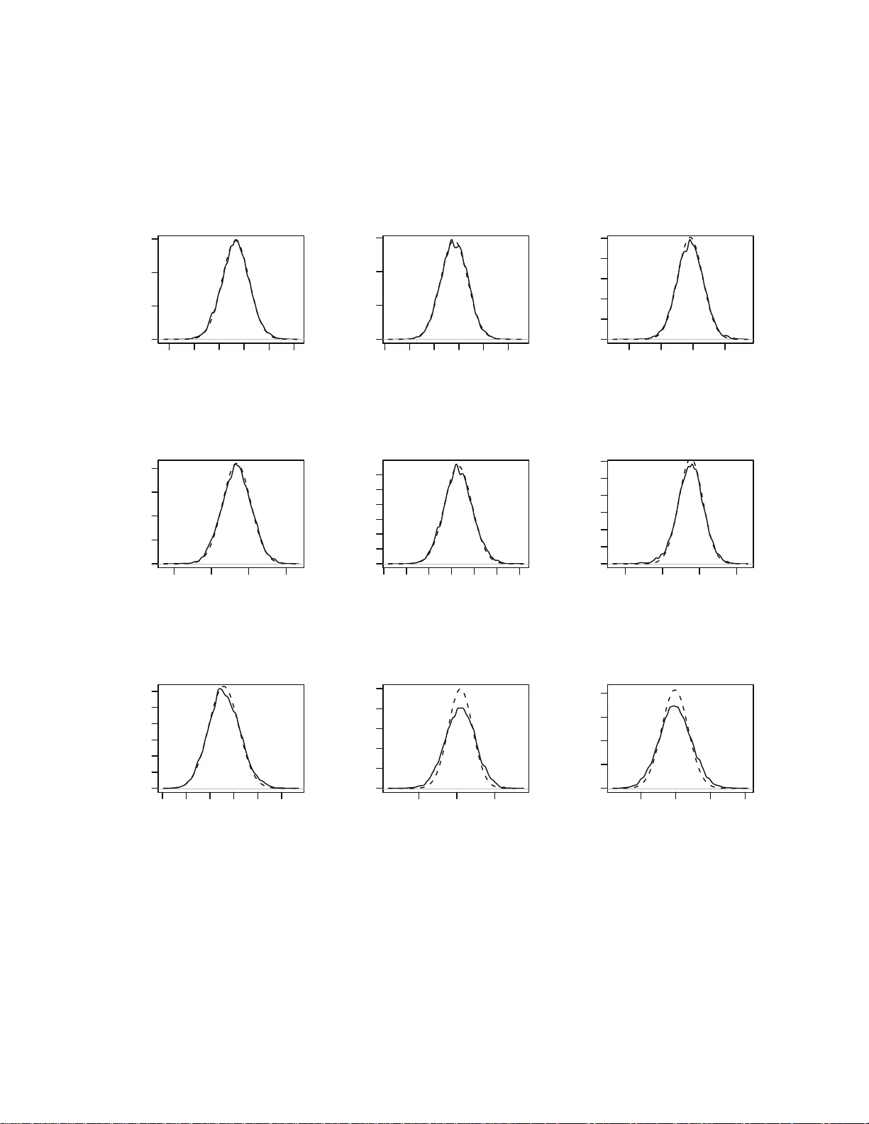
V ariational appro ximation for heteroscedastic linear mo dels and matc hing pursuit algo rithms Da vid J. Nott, Minh-Ngo c T r an, Chenlei Leng ∗ Abstract Mo dern statistica l applications inv olving large data sets hav e fo cused attent ion on statistica l metho dolog ies whic h are b o th efficien t computational ly and able to deal with the screening of large num b ers of differen t candidate mod e ls. Here w e consider com- putationally efficien t v a riational Ba y es app roa c hes to in ference in high-dimen s i onal het- eroscedastic linear regression, where b oth the mean and v ariance are d esc rib ed in terms of linear fun ct ions of the p redicto rs and where the num b er of predictors can b e larger than the sample size. W e deriv e a closed form v ariatio nal lo w er b ound on the log marginal lik eliho od u seful for mo del selection, and p ropose a no ve l fast greedy searc h algorithm on the m o del space w hic h m akes use of one-step optimizatio n u p dates to the v aria tional lo w er b ound in the curr e nt mo del for screening large num b ers of candid a te predictor v a riables for inclus ion/exclusion in a compu ta tionally thr if ty wa y . W e show that the model searc h strategy w e suggest is related to widely us e d orthogonal m a tc hing pursu i t algorithms for mo del searc h bu t yields a framew ork for p oten tially extendin g these algorithms to more complex mo dels. The metho dolog y is applied in simulatio ns and in t w o real examples in v olving pr e diction for fo od constituents using NIR tec hnology and prediction of disease p rog ression in diab etes. Keyw ords. Ba y esian mo del selection, heteroscedasticit y , matc hing p ursuit, v ariational appro ximation. ∗ David J. Nott and Chenlei Leng a re Asso ciate Professo r s, Minh-Ngo c T r a n is PhD candidate at Depar t- men t of Statistics and Applied Pro babilit y , National Universit y of Singap ore, Singap ore 1175 46, Republic of Singap ore. Corre sponding author: Minh-Ngo c T ran (ngo ctm@nus.edu.sg). 1 1 In tro ductio n Consider the heteroscedastic linear regression mo del y i = x T i β + σ i ǫ i , i = 1 , . . . , n (1) where y i is a resp onse, x i = ( x i 1 ,...,x ip ) T is a corresp onding p -ve ctor of predictors, β = ( β 1 ,...,β p ) T is a v ector of unkno wn mean parameters, ǫ i ∼ N (0 , 1) are indep enden t error s and log σ 2 i = z T i α, where z i = ( z i 1 ,...,z iq ) T is a q -v ector of predictors and α = ( α 1 ,...,α q ) T are unkno wn v ariance parameters. In this mo del the standard deviation σ i of y i is b eing mo d eled in terms of the predictors z i ; this heteroscedastic mo del ma y b e con trasted with the usual homoscedastic mo del whic h assumes σ i is constant. W e take a Bay esian approac h to inference for this mo del and consider a prior distribution p ( θ ) on θ = ( β T ,α T ) T of the form p ( θ ) = p ( β ) p ( α ) with p ( β ) and p ( α ) b oth normal, N ( µ 0 β , Σ 0 β ) and N ( µ 0 α , Σ 0 α ) resp e ctiv ely . It is p ossible to consider hierarchical extensions for the priors on p ( β ) and p ( α ) but w e do not consider this here. W e will consider a v ariationa l Ba y es approach fo r inference (see Section 2 for the details). The term v ariational appro ximation refers t o a wide ra nge of differen t metho ds where the idea is to con vert a problem of integration into an optimization problem. In Bay esian inference, v ariational approx imation provide s a fast alternativ e to Monte Carlo metho ds fo r approxi- mating p osterior distributions in complex mo dels, esp ecially in high-dimensional problems. In the heteroscedastic linear regression mo del, w e will consider a v ariational appro ximation to the joint p osterior distribution o f β and α a s q ( β ,α ) = q ( β ) q ( α ), where q ( β ) and q ( α ) are b oth normal densities, N ( µ q β , Σ q β ) a nd N ( µ q α , Σ q α ) r esp ectiv ely . It is also p ossible to giv e a v a ri- ational treatmen t in whic h independence is not assumed b et w een β and α (John Ormero d, p ersonal comm unicatio n) but this complicates the v ariational optimization somewhat. W e at- tempt to c ho ose t h e parameters in the v ariational p o s terior µ q β , µ q α , Σ q β and Σ q α to minimize the Kullbac k-Leibler div ergence b et wee n the t rue p osterior distribution p ( β ,α | y ) and q ( β ,α ). This results in a lo w er b ound on the log marg ina l lik eliho o d log p ( y ) - a ke y quantit y in Bay esian 2 mo del selection. The first contribution of our pap er is the deriv ation of a closed form for the lo w er b ound and the prop osal of an iterativ e sc heme for maximizing it. This low er b ound maximization pla ys a crucial r o le in the v ariable selection pro blem discussed in Section 3. V ariable selection is a fundamen tal problem in statistics and mac hine learning, and a la r g e n um b er of metho ds hav e b een prop osed for v aria ble selection in homoscedastic regression. The traditional v ariable selection a p proach in the Bay esian framew ork consists of building a hierarchical Bay es mo del and using MCMC algor ithm s to estimate p osterior mo del prob- abilities (George and McCullo c h, 1993 ; Smith and Kohn, 1996; Raftery et al., 1997). This metho dology is computationally demanding in high-dimensional problems and there is a need for fast alternativ es in some applications. In high-dimensional settings, a lte rnative approache s include t he family of greedy algo rithms (T ropp, 2 0 04 ; Zhang, 2009), also know n as matching pursuit (Mallat a nd Zhang, 1993) in signal pro cessing. Greedy alg o rithms are closely related to the Lasso (Tibshirani , 1996) and the LARS a lgorithm (Efron et a l., 2004). See Zhao and Y u (2007); Efron et al. (20 0 4 ) and Zhang (2 009 ) for excellen t comparisons of these families of al- gorithms. In the statistical contex t, g r eedy algo rithms hav e b een pro v en to b e v ery efficien t for v ariable selection in linear regr ession under the assumption of homoscedasticit y , i.e. where the v ariance is assumed to b e constan t (Zhang, 20 09 ). In many applicatio ns the assumption of constan t v ariance may b e unrealistic. Ignor in g het- eroscedasticit y ma y lead to serious problems in inference, suc h a s misleading assessmen ts of sig- nificance, p o or predictiv e p erformance and inefficien t estimation of mean parameters. In some cases, learning the structure in the v ariance ma y b e the primary goal. See Chan et al. (2006), Carroll and Rupp ert (1988) and Rupp ert et al. (2 0 03 ), Chapter 14, for a more detailed discus- sion on heteroscedastic mo deling. Despite a large n um b er of w orks on heteroscedastic linear regression and o v erdisp ersed generalized linear mo dels in whic h ov erdisp ersion is mo deled to dep end on the cov ar iates (Efron, 198 6 ; Nelder and Pregib on, 1 9 87 ; Davidian and Carro ll , 1987; Sm yth , 19 8 9 ; Y ee and Wild, 1996 ; Rig b y and Stasinop oulos, 2005), metho ds for v a r i- able selection seem to b e somewhat ov erlo ok ed. Y a u and Kohn (20 0 3 ) and Chan et al. (2006) consider Ba y esian v ariable selection using MCMC computational approa c hes in heteroscedas- 3 tic Gaussian mo dels. They discuss extensions in v olving flexible mo deling of the mean a nd v ariance functions. Cottet et al. (2008) consider extensions to ov erdisp erse d generalized lin- ear and generalized additiv e mo dels. These approaches are computationally demanding in high-dimensional settings. A general and flexible f r ame w ork for mo deling ov erdisp erse d data is a ls o considered by Y ee and Wild (1 996 ) and Rigby a n d Stasinop oulos (2005). Metho ds for mo del selection, how ev er, are less w ell dev elop ed. A common approac h is to use info rma- tion criteria suc h as generalized AIC and BIC tog e ther with forward step wise metho ds (see, for example, Rigb y and Stasinop oulos ( 2 005), Section 6). W e compare our o wn approac hes to suc h metho ds later. A main contribution of the presen t pap er is to prop ose a no v el fast greedy alg orithm for v ariable selection in heteroscedastic linear regression. W e sho w that the prop osed algorithm is in homoscedastic cases similar to curren tly used metho ds while ha ving man y attr a c tiv e prop erties and w orking efficien tly in high-dimensional problems. An efficien t R program is av aila ble on the authors’ webs ites. In Section 4 we apply our a lg orithm to the analysis of the diab etes data (Efron et al., 20 0 4 ) using heteroscedastic linear regression. This data set consists of 64 predictors (constructed from 10 input v ariables for a “quadratic mo del”) and 442 observ ations. W e sho w in Figure 1 the estimated co effi cien ts corresp onding to selected predictors as functions o f iteratio n steps in our a lg orithm, for b oth the mean and v ariance mo dels. The algorithm stops after 1 1 forw ard selection steps with 8 a nd 7 predictors selected for the mean and v a riance mo dels resp ectiv ely . The rest of the pap er is organized as f ollo ws. The closed form o f the low er b ound and the iterativ e sc heme for maximizing it are presen ted in Section 2. W e presen t in Section 3 our no v el fast greedy algorithm, and compare it to existing greedy a lgorithms in the literature for homoscedastic regression. In Section 4 w e apply our metho dology to the a naly sis of tw o b enc hmark data sets. Exp erime ntal studies a re presen ted in Section 5. Section 6 con tains conclusions and future researc h. T ec hnical deriv ation is relegated to the App endices. 4 2 4 6 8 10 −2000 −1000 0 1000 2 2 4 6 8 10 −2000 −1000 0 1000 3 2 4 6 8 10 −2000 −1000 0 1000 4 2 4 6 8 10 −2000 −1000 0 1000 9 2 4 6 8 10 −2000 −1000 0 1000 11 2 4 6 8 10 −2000 −1000 0 1000 12 2 4 6 8 10 −2000 −1000 0 1000 28 2 4 6 8 10 −2000 −1000 0 1000 Mean model steps estimated coefficients 40 2 4 6 8 10 0 10 20 30 2 2 4 6 8 10 0 10 20 30 3 2 4 6 8 10 0 10 20 30 4 2 4 6 8 10 0 10 20 30 9 2 4 6 8 10 0 10 20 30 11 2 4 6 8 10 0 10 20 30 12 2 4 6 8 10 0 10 20 30 V ariance model steps estimated coefficients 40 Figure 1: Solution paths as f unctions of iteration steps for a naly zing the diab etes data using heteroscedastic linear regression. The algo r it h m stops aft er 11 iterations with 8 and 7 predic- tors selected fo r the mean and v a riance mo dels resp ectiv ely . The selected predictors en ter the mean (v aria nce) mo del in the order 3, 12, ..., 28 (3, 9, ..., 4). 2 V ariational Ba y es W e now g ive a brief introduction to the v a riational approximation metho d. F or a mor e de- tailed exposition see, for example, Jordan et al. (1999), Bishop (2006) Chapter 10, or see Ormero d and W and ( 2009) for a statistically oriented in tro duction. The term v ariat io nal ap- pro ximation refers to a wide range o f differen t metho ds where the idea is to conv ert a problem of in tegration in to an optimization problem. Here w e will only b e concerned with applications of v ariationa l metho ds in Bay esian inf erence and only with a particular approach sometimes referred to as parametric v aria tional approx imation. W rite θ for all our unkno wn parameters, p ( θ ) for the prior distribution and p ( y | θ ) for t he lik eliho o d. F or Ba y esian inference, decisions 5 are based on the p osterior distribution p ( θ | y ) ∝ p ( θ ) p ( y | θ ). A common difficult y in applications is how to compute quantitie s of in terest with resp ec t to the p osterior. These computations often inv olve the ev aluation of high-dimensional in tegrals. V ariational appro ximation pro - ceeds by a pproximating the p oste rior distribution directly . F ormally , w e consider a family of distributions q ( θ | λ ) where λ denotes some unknow n parameters, and att e mpt to choose λ so that q ( θ | λ ) is closest to p ( θ | y ) in some sens e. In pa r tic ular, w e attempt to minimize the Kullbac k-Leibler divergenc e Z log q ( θ | λ ) p ( θ | y ) q ( θ | λ ) dθ with resp ect to λ . Using the iden tity log p ( y ) = Z log p ( θ ) p ( y | θ ) q ( θ | λ ) q ( θ | λ ) dθ + Z log q ( θ | λ ) p ( θ | y ) q ( θ | λ ) dθ, (2) where p ( y ) = R p ( θ ) p ( y | θ ) dθ , w e see that minimizing the Kullback-Leibler div ergence is equiv- alen t to the maximization o f Z log p ( θ ) p ( y | θ ) q ( θ | λ ) q ( θ | λ ) dθ. (3 ) Here (3) is a low er b ound (often called t he free energy in ph ysics) on the log marginal lik eliho o d log p ( y ) due t o the non-negativit y of the Kullback-Leibler div ergence term in (2). The lo w er b ound (3), when maximized with resp ect to λ , is o ften used as an a p proximation to the log marginal lik eliho o d log p ( y ). The erro r in the approximation is the Kullbac k-Leibler div ergence b et we en the a ppro ximation q ( θ | λ ) and the true p osterior. The appro ximation is useful, since log p ( y ) is a k ey quantit y in Bay esian mo del selection. F or our heteroscedastic linear mo del, the low er b ound (3) can b e expressed as L = T 1 + T 2 + T 3 , where T 1 = Z log[ p ( β , α )] q ( β ) q ( α ) dβ dα, T 2 = Z log[ p ( y | β , α )] q ( β ) q ( α ) dβ dα, T 3 = − Z log [ q ( β ) q ( α )] q ( β ) q ( α ) d β dα. 6 W e sho w (see the App endix A) that these three terms, whic h are all exp ectations with resp ec t to the (assumed normal) v a riational p osterior, can b e ev aluated analytically . Putting the terms together we obtain that the lo w er b ound (3) on the log margina l lik eliho o d is L = p + q 2 − n 2 log 2 π + 1 2 log | Σ q β Σ 0 β − 1 | + 1 2 log | Σ q α Σ 0 α − 1 | − 1 2 tr(Σ 0 β − 1 Σ q β ) − 1 2 tr(Σ 0 α − 1 Σ q α ) − 1 2 ( µ q β − µ 0 β ) T Σ 0 β − 1 ( µ q β − µ 0 β ) − 1 2 ( µ q α − µ 0 α ) T Σ 0 α − 1 ( µ q α − µ 0 α ) − 1 2 n X i =1 z T i µ q α − 1 2 n X i =1 ( y i − x T i µ q β ) 2 + x T i Σ q β x i exp  z T i µ q α − 1 2 z T i Σ q α z i  . (4) This needs to b e maximized with resp ect to µ q β , µ q α , Σ q β , Σ q α . W e consider an iterativ e sc heme in whic h w e maximize with resp ec t to each of the blo c ks of par ame ters µ q β , µ q α , Σ q β , Σ q α with the other blo c ks held fixed. W rite X for the design matrix with i th row x T i and D for the diago na l matr ix with i th diagonal elemen t 1 / e xp( z T i µ q α − 1 2 z T i Σ q α z i ). Maximization with resp ect to µ q β with other terms held fixed leads to µ q β =  X T D X + Σ 0 β − 1  − 1  Σ 0 β − 1 µ 0 β + X T D y  . Maximization with resp ect to Σ q β with other terms held fixed leads to Σ q β =  Σ 0 β − 1 + X T D X  − 1 . Handling the parameters µ q α and Σ q α in the v ariatio nal p osterior for α is more complex. W e pro cee d in the follo wing w a y . If no parametric f orm for the v ariatio nal p osterior q ( α ) is assumed (that is, if w e do not a s sume that q ( α ) is normal) but only assume the factor- ization q ( θ ) = q ( β ) q ( α ) then the optimal c ho ic e for q ( α ) for a giv en q ( β ) = N ( µ q β , Σ q β ) is (see Ormero d and W and (20 0 9 ), for example) q ( α ) ∝ exp  E (lo g [ p ( θ ) p ( y | θ )])  , (5) where the exp ectation is with resp ect to q ( β ). Similar to the deriv a tion of the low er b ound (4), it is easy to see that q ( α ) ∝ exp − 1 2 n X i =1 z T i α − 1 2 n X i =1 ( y i − x T i µ q β ) 2 + x T i Σ q β x i exp( z T i α ) − 1 2 ( α − µ 0 α ) T Σ 0 α − 1 ( α − µ 0 α ) ! , 7 whic h ta k es the fo rm of the p osterior (apart fr o m a normalization constan t) for a Ba y esian generalized linear mo del with g a m ma resp onse and log link, co efficien t of v a r iation √ 2, a nd resp ons es w i = ( y i − x T i µ q β ) 2 + x T i Σ q β x i with the log of the mean resp onse b eing z T i α . The prior in this gamma generalized linear mo del is N ( µ 0 α , Σ 0 α ). If we use a quadratic a pp roximation to lo g q ( α ) then this results in a normal approximation to q ( α ) . W e c ho ose the mean and v ariance of the normal a pp roximation simply b y the p osterior mo de and the negativ e in v erse Hessian of the log p oste rior at the mo de for the ga m ma generalized linear mo del described ab o v e. The computations required are standard ones in fitting a Ba y esian generalized linear mo del (see App endix B) . W rite Z for the design matrix in the v aria nce mo del with i th ro w z T i and write W ( α ) (as a function of α ) f o r the diagonal matrix diag ( 1 2 w i exp( − z T i α )). With µ q α the p osterior mo de, w e obtain f o r Σ q α the expression Σ q α =  Z T W ( µ q α ) Z + Σ 0 α − 1  − 1 . Our optimization ov er µ q α and Σ q α is only appro ximate, so that we only r eta in the new v alues in the optimization if they result in an improv emen t in the low er b ound (4). The adv antage of our appro ximate approac h is the closed fo rm express ion for the up date of Σ q α once µ q α is found, so that explicit n umerical optimization for a p ossib ly high-dimensional co v ariance ma t r ix is a v oided. The explicit a lgorithm for our metho d is the following. Algorithm 1: Maximization of the v ariational lo w er b ound. 1. Initialize par ame ters µ q α , Σ q α . 2. µ q β ←  X T D X + Σ 0 β − 1  − 1  Σ 0 β − 1 µ 0 β + X T D y  where D is the diagonal matrix with i th diagonal en try 1 / exp  z T i µ q α − 1 / 2 z T i Σ q α z i  . 3. Σ q β ←  X T D X + Σ 0 β − 1  − 1 . 4. Obtain µ q α as the p osterior mo de for a gamma generalized linear mo del with normal prior N ( µ 0 α , Σ 0 α ), gamma resp onses w i = ( y i − x T i µ q β ) 2 + x T i Σ q β x i , co efficien t of v ariation √ 2 and where the log of the mean is z T i α . 8 5. Σ q α ←  Z T W Z + Σ 0 α − 1  − 1 where W is diago nal with i th diagonal elemen t w i exp( − z T i µ q α ) / 2. 6. If the up dates done in steps 3 and 4 do not impro v e the low er b ound (4) then their old v alues are r eta ined. 7. Rep eat steps 2 - 6 until the increase in the v ariat io nal low er b ound (4) is less than some user sp ec ified tolerance. F or initialization, we first p erform an ordinar y least squares (OLS) fit for the mean mo del to get a n estimate ˆ β of β . Then w e take the residuals from this fit, say r i = ( y i − x T i ˆ β ) 2 , and do an OLS fit of log r i to the predictors z i to obtain our initial estimate of µ q α . The initial v alue of Σ q α is then set to the co v ar ia nc e matrix of the least squares estimator. When the OLS fits are no t v alid, some other metho d suc h as the Lasso can b e used instead. The application of this algo rithm to the problem of v ariable selection in Section 3 alw a ys in v olv es only situations in whic h the ab o v e OLS fits are a v aila ble. W e men tion one further extension of our metho d. W e ha v e a s sumed ab o v e that t he prior co v ariance matrices Σ 0 β and Σ 0 α are kno wn. Later we will assume Σ 0 β = σ 2 β I and Σ 0 α = σ 2 α I where I denotes the iden tity matrix and σ 2 β and σ 2 α are scalar v ariance parameters. W e further assume that µ 0 β = 0 and µ 0 α = 0. It may b e helpful to p erform some data drive n shrink ag e so that σ 2 β and σ 2 α are considered unkno wn and to b e estimated from the data. Our low er b ound (4) can b e considered as an approximation to log p ( y | σ 2 β ,σ 2 α ), and the log p osterior for σ 2 β ,σ 2 α is apart from an additiv e constan t log p ( σ 2 β , σ 2 α ) + log p ( y | σ 2 β , σ 2 α ) . If we assume indep enden t in v erse gamma prio rs , I G ( a,b ), for σ 2 β and σ 2 α , and if w e replace the log marginal lik eliho o d b y the lo w er b ound and maximize, we get σ 2 β = b + 1 2 µ q β T µ q β + 1 2 tr(Σ q β ) a + 1 + p/ 2 and σ 2 α = b + 1 2 µ q α T µ q α + 1 2 tr(Σ q α ) a + 1 + q / 2 . These up dating steps can b e added to the Algorithm 1 giv en a b ov e. 9 3 Mo del sele ction In the discuss ion of the previous sections the c hoice of predictors in the mean and v a r ia nc e mo dels was fixed. W e now consider the problem of v ariable selection in the heteroscedastic linear mo del, and the question of computationally efficien t mo del searc h when the num b er of candidate predictors is v ery large, p erhaps m uc h larger than the sample size. In Sections 1 and 2 w e denoted the marginal lik eliho o d b y p ( y ) without making explicit conditioning on the mo del but now we write p ( y | m ) for the marginal likelihoo d in a mo del m . If w e ha v e a prior distribution p ( m ) on the set of all mo dels under consideration then Bay es’ rule leads t o the p osterior distribution on the mo del given b y p ( m | y ) ∝ p ( m ) p ( y | m ). W e can use the v ariatio n al lo w er b ound on log p ( y | m ) as a replacemen t for log p ( y | m ) in this formula as one strategy for Ba y esian v a riable selection when p ( y | m ) is difficult to compute. W e follow that strategy here. F or a more thorough review of the Bay esian approach to mo del selection see, for example, O’Hagan and F orster (2004). Using the maximized lo w er b ound is a p opular approac h for mo del selection (Beal and G ha hramani , 2003, 2006; W u et al., 2010). The error in using the lo w er b ound to appro ximate log p ( y | m ) is the Kullback-Leible r divergenc e betw een the true p osterior p ( θ | y ) a nd the v ariational distri- bution q ( θ | λ ). The true p osterior in our mo del ha s the structure of a pro duct of tw o normal distributions a nd the v ariatio na l distribution w e use is also a pro duct of t w o no rmals . There- fore, it can b e exp ected that the minimized KL div ergence is small, thus leading to a go od appro ximation. The exp erime ntal study in Section 5 suggests that the maximized low er b ound is v ery tig h t. Before presen ting our strategy for ranking v ariational low er b ounds, we discuss here the mo del prio r. Supp ose we ha v e a current mo del with predictors x i , i ∈ C ⊂ D = { 1 ,...,p } in the mean mo del and z i , i ∈ V ⊂ E = { 1 ,...,q } in the v a riance mo del. The subsets C and V give indices for the curren tly activ e predictors in the mean and v ariance mo dels. Let π µ i ( π σ j ) b e the prior probabilit y for inclusion of x i ( z j ) in the mean (v ariance) mo del, and write π µ = ( π µ 1 ,...,π µ p ) T , 10 π σ = ( π σ 1 ,...,π σ q ) T . W e assume that the inclusions of predictors are indep end en t a priori with p ( C | π µ ) = Y i ∈ C π µ i Y i 6∈ C (1 − π µ i ) , p ( V | π σ ) = Y j ∈ V π σ j Y j 6∈ V (1 − π σ j ) , and the prior probability of a mo del m with index sets C and V in its mean and v aria nce mo dels is a s sumed to b e p ( m ) = p ( C, V | π µ , π σ ) = p ( C | π µ ) p ( V | π σ ) . (6) If no suc h detailed prior information is a v a ila ble for each individual predictor (which is the situation w e consider in this pap er), one may assume that π µ 1 = ... = π µ p = π µ and π σ 1 = ... = π σ q = π σ (w e note a slight abuse of notat io n here). Then p ( C | π µ ) = π | C | µ (1 − π µ ) p −| C | , p ( V | π σ ) = π | V | σ (1 − π σ ) q −| V | , (7) where h yp e rparameters π µ , π σ ∈ [0 , 1 ] are user-sp ecified. One can encourage parsimonious mo dels b y setting small ( < 1 / 2) π µ and π σ . T he smaller the π µ and π σ , the smaller prio r probabilities are put on complex mo dels. By setting π µ = π σ = 1 / 2, one can set a uniform prior on the mo dels. Another option is to put uniform distributions on π µ and π σ . Then p ( C ) = Z 1 0 p ( C | π µ ) dπ µ ∝  p | C |  − 1 , p ( V ) = Z 1 0 p ( V | π σ ) dπ σ ∝  q | V |  − 1 . (8) This prior agrees with the o ne used in the extended BIC prop osed b y Chen and Chen (2008). It has the adv a n tage of r equiring no h yp e rparameter while still encouraging parsimony . W e recommend using this as the default prior. W e no w consider adding a single v a riable in either the mean o r the v ariance mo de l, and then a o ne-step up date to the curren t v ariational low er b ound in the prop osed mo del as a computationally thr if t y wa y of ranking the predictors for p ossible inclusion. In our one-step up date, w e consider a v aria t ional approx imation in which the v ariational p osterior distribution factorizes in to separate parts for t he added parameter and the parameters in t he curren t mo del, as w ell as the factorization of mean and v ariance parameters in Section 2. W e stress that this factorization is only assumed for the purp ose of ranking predictors for inclusion. Once a v ariable has b een selected fo r inclusion, the p osterior distribution is approximated using the 11 metho d outlined in Section 2. W rite β C for the para meters in the curren t mean mo de l and X C for the corresp onding design matrix, and α V for the para meters in the curren t v ariance mo del with Z V the corresp onding design matrix. W rite x C i for the i th row of X C and z V i for the i th row o f Z V . 3.1 Ranking predictors in the mean mo del Let us consider first the effect of adding the predictor x j , j ∈ D \ C , to the mean mo del. W e write β j for the co efficien t of x j and we consider a v ariat io nal approximation to the p osterior of the form q ( θ ) = q ( β C ) q ( β j ) q ( α V ) , (9) with q ( β C ) = N ( µ q β C , Σ q β C ), q ( α V ) = N ( µ q αV , Σ q αV ) and q ( β j ) = N ( µ q β j , ( σ q β j ) 2 ). Supp ose that w e ha v e fitt ed a v ariatio nal approximation for the current mo del (i.e. the mo de l without x j ) using the pro cedure of Section 2. W e now consider fitting the extended mo del with µ q β C , Σ q β C ,µ q αV and Σ q αV fixed a t the optimized v a lue s obtained for the curren t mo del, and consider just one step of a v ariational algorithm for ma ximizing t h e v ariational low er b ound in the new mo del with resp ect to the parameters µ q β j , ( σ q β j ) 2 . In effect for our v ariational lo w er b ound (4), w e are assuming that the v a riational p oste rior distribution for ( β C T ,β j ) T is normal with mean ( µ q β C T ,µ q β j ) T and cov ariance matrix " Σ q β C 0 0 ( σ q β j ) 2 # . Substituting these forms into (4) a n d further assuming µ 0 β = 0, µ 0 α = 0, Σ 0 β = σ 2 β I and Σ 0 α = σ 2 α I (see the remarks at the end o f Section 2), w e obtain the low er b ound L = L old + 1 2 + 1 2 log ( σ q β j ) 2 σ 2 β − ( σ q β j ) 2 2 σ 2 β − ( µ q β j ) 2 2 σ 2 β − 1 2 n X i =1 x 2 ij ( σ q β j ) 2 + x 2 ij ( µ q β j ) 2 − 2 x ij µ q β j ( y i − x T C i µ q β C ) exp  z T iV µ q αV − 1 2 z T iV Σ q αV z iV  , (10) where L old is the previous low er b ound for the curren t mo del without predictor j . Here w e are writing x ij for the v alue of predictor j for observ at ion i . Optimizing t he ab o v e b ound with 12 resp e ct to µ q β j and ( σ q β j ) 2 and writing ˆ µ q β j and ( ˆ σ q β j ) 2 for the optimizers giv es ˆ µ q β j = n X i =1 x ij ( y i − x T C i µ q β C ) exp  z T V i µ q αV − 1 2 z T V i Σ q αV z V i  ! . 1 σ 2 β + n X i =1 x 2 ij exp  z T V i µ q αV − 1 2 z T V i Σ q αV z V i  ! (11) and ( ˆ σ q β j ) 2 = 1 σ 2 β + n X i =1 x 2 ij exp  z T V i µ q αV − 1 2 z T V i Σ q αV z V i  ! − 1 . (12) Substituting these back in to the lo w er b ound (10) giv es L old + 1 2 log ( ˆ σ q β j ) 2 σ 2 β + 1 2 ( ˆ µ q β j ) 2 ( ˆ σ q β j ) 2 . (13) If the v ariance mo del contains only an interc ept, this result agrees with greedy selection algorithms where predictors are rank ed according to the correlation b et w een a predictor and the residuals f rom the curren t mo del (see, e.g. Zhang (20 09 )). W e will discuss this p oin t in detail in Section 3.5. Later w e write t h e optimized v alue of (10) as L M j ( C ,V ), the sup ers cript M means the lo w er b ound asso ciated with the mo del f o r m ean. 3.2 Ranking predictors in the v ariance mo del So far w e hav e considered only the a dditio n of a predictor in the mean mo del. W e now attempt a similar analysis o f the effect o f inclusion of a predictor in the v aria nc e mo de l. With the mean mo del fixed, supp ose that w e are considering adding a predictor z j , j ∈ E \ V , to the v ariance mo del. W e consider a normal approximation to the p osterior q ( θ ) = q ( β C ) q ( α V ) q ( α j ) with q ( β C ) = N ( µ q β C , Σ q β C ), q ( α V ) = N ( µ q αV , Σ q αV ) and q ( α j ) = N ( µ q αj , ( σ q αj ) 2 ). The v ariational lo w er b ound is L old + 1 2 + 1 2 log ( σ q αj ) 2 σ 2 α − ( σ q αj ) 2 2 σ 2 α − ( µ q αj ) 2 2 σ 2 α − 1 2 X i z ij µ q αj − 1 2 n X i =1 ( 1 exp( z T V i µ q αV − 1 2 z T V i Σ q αV z V i + z ij µ q αj − 1 2 z 2 ij ( σ q αj ) 2 ) − 1 exp( z T V i µ q αV − 1 2 z T V i Σ q αV z V i ) ) ×  ( y i − x T C i µ q β C ) 2 + x T C i Σ q β C x C i  , (14) where L old is the lo w er b ound for the curren t mo del without predictor z j . T o obtain go o d v alues fo r µ q αj and ( σ q αj ) 2 , we use an approximation similar to the one used fo r the v a riance 13 parameters in Section 2 . If we do not assume a no r m al form fo r q ( α j ) but just the factorization q ( θ ) = q ( β C ) q ( α V ) q ( α j ) and with the curren t q ( β C ) and q ( α V ) fixed, then the optimal q ( α j ) is q ( α j ) ∝ exp( E (log p ( α j ) + log p ( y | θ ))) , where the exp ectation is with resp ec t to q ( β C ) q ( α V ). W e ha v e that E (lo g p ( α j ) + log p ( y | θ )) = E − 1 2 log 2 π − 1 2 log σ 2 α − α 2 j 2 σ 2 α − n 2 log 2 π − 1 2 n X i =1 z T V i α V − 1 2 n X i =1 z ij α j − 1 2 n X i =1 ( y i − x T C i β C ) 2 exp ( z T V i α V + z ij α j ) ! = − 1 2 log 2 π − 1 2 log σ 2 α − α 2 j 2 σ 2 α − n 2 log 2 π − 1 2 n X i =1 z T V i µ q αV − 1 2 n X i =1 z ij α j − 1 2 n X i =1 ( y i − x T C i µ q β C ) 2 + x T C i Σ q β C x C i exp  z T V i µ q αV + z ij α j − 1 2 z T V i Σ q αV z V i  . (15) W e mak e a normal a pp roximation N ( ˆ µ q αj , ( ˆ σ q αj ) 2 ) to the optimal q ( α j ) via the mo de and negativ e inv erse second deriv ative of (15). Differen tiating with resp ec t to α j , w e obtain − α j σ 2 α − 1 2 n X i =1 z ij + 1 2 n X i =1 z ij v i exp( z ij α j ) where v i = ( y i − x T C i µ q β C ) 2 + x T C i Σ q β C x C i exp  z T V i µ q αV − 1 2 z T V i Σ q αV z V i  . Appro ximating exp( − z ij α j ) ≈ 1 − z ij α j (i.e. using a T ay lor series expansion ab out zero), setting the deriv ative to zero and solving giv es ˆ µ q αj = 1 2 n X i =1 z ij ( v i − 1) ! . 1 σ 2 α + 1 2 n X i =1 z 2 ij v i ! . (16) T o g e t more accurate estimation of the mo de, some optimization pro cedu re ma y b e used here with (16) used a s an initial p oin t. I n our R implemen ta tion, the Newton metho d w as used b ecaus e (15) has its second deriv ativ e a v ailable in a closed form (see (17) b elo w). W e found that (16) is a v ery g oo d appro ximation as t he Newton iteratio n v ery often stops after a small n um b er of iterations (with a stopping tolerance as small as 10 − 10 ). Differen tiating (15) once more, and finding the negativ e inv erse of t he second deriv a tiv e at ˆ µ q αj giv es ( ˆ σ q αj ) 2 = 1 σ 2 α + 1 2 n X i =1 z 2 ij v i exp( z ij ˆ µ q αj ) ! − 1 . (17) 14 W e can plug t hese v alues bac k into the lo w er b ound in order to rank different predictors for inclusion in the v ariance mo del. Once again we note the computationally thrift y nature of the calculations. W e write the o pt imized v alue of (14) as L D j ( C ,V ), the sup erscript D means the low er b ound asso ciated with t he mo del for standard d eviance. 3.3 Summary of the algorit hm W e summarize our v ariable selection algorithm b elo w. W e write L ( C ,V ) for the optimized v alue of the low er b ound (4) with the predictor set C in the mean mo del and the predictor set V in the v ariance mo del. W rite C + j for the set C ∪ { j } and V + j for the set V ∪ { j } . Algorithm 2: V ariational appro ximation ranking (V AR) algorithm. 1. Initialize C and V a nd set L opt := L ( C ,V ). 2. Rep eat the following steps un til stop (a) Store C old := C , V old := V . (b) Let j ∗ = argmax j { L M j ( C ,V ) + log p ( C + j ,V ) } . If L ( C + j ∗ ,V ) + lo g p ( C + j ∗ ,V ) > L opt + log p ( C ,V ) } then set C := C + j ∗ , L opt = L ( C + j ∗ ,V ). (c) Let j ∗ = a rgmax j { L D j ( C ,V ) + log p ( C,V + j ) } . If L ( C ,V + j ∗ ) + log p ( C,V + j ∗ ) > L opt + log p ( C ,V ) then set V := V + j ∗ , L opt = L ( C ,V + j ∗ ). (d) If C = C old and V = V old then stop, else return to (a). 3.4 F orw ard-bac kw ard ranking algorithm The ranking algorithm describ ed ab o v e can b e regarded as a forw ard greedy a lgorithm b ecause it considers adding at eac h step another predictor to the curren t mo del. Hereafter w e refer to this algorithm as forw ard v ariational ra nking algo r it h m or fV AR in short. Lik e the other forw ard greedy algo rithms that hav e b een widely used in man y scien tific fields, the fV AR w orks well in most of the examples tha t w e ha v e encoun tered. How ev er, a ma jor drawbac k 15 with the forw ard selection algo rithms is that if a predictor has b een wrongly selected t hen it can not b e r emov ed any more. A natural remedy for this is to add a backw ard elimination pro cess in order to corr e ct mistake s made in the earlier forward selection. W e presen t here a recip e for r a nk ing predictors for exclusion in the mean and v ar ia nc e mo dels. Let C , V b e the current sets of predictors in the mean and v aria nce mo dels resp ec tive ly . With j ∈ C , we write C − j for the set C \ { j } and consider now the effect o f remo ving the predictor x j to the low er b ound. In or d er to reduce computational burden, w e need some wa y to a v oid the need to do low er b o un d maximization f or eac h mo del C − j when ranking x j for exclusion. Similar as b efore, w e consider a v ariatio na l appro ximation using the factorizatio n (9) for the v ariational p osterior distribution. F ollo wing steps (10)-(13), we can approximately write the lo w er b ound for the curren t mo del (i.e. the mo del con tains x j ) as the sum of the lo w er b ound for the mo del without x j and a x j -based term L ( C, V ) ≈ L ( C − j , V ) + Γ M C − j ,V ( j ) , (18) with Γ M C − j ,V ( j ) := 1 2 log ( ˆ σ q β j ) 2 σ 2 β + 1 2 ( ˆ µ q β j ) 2 ( ˆ σ q β j ) 2 , (19) where ˆ µ q β j , ˆ σ q β j are as in (11) and (12) with C replaced by C − j . All the relev an t quantities needed in the calculation of Γ M C − j ,V ( j ) are fixed at o ptimiz ed v alues maximizing the low er b ound for the current mo del. The subscripts C − j ,V emphasize that the quan tities needed are adjusted corresp ondingly when the predictor j is remov ed from the mean mo del. The most plausible candidate fo r exclusion from the curren t mean mo del then is j ∗ = argmax j ∈ C { L ( C − j , V ) + log p ( C − j , V ) } = argmin j ∈ C { Γ M C − j ,V ( j ) − log p ( C − j , V ) } . (20) W e now rank the predictors for exclusion in the v aria nc e mo del. F ollowing the argumen ts in Section 3.2 and the ab o v e, we can write L ( C, V ) ≈ L ( C , V − j ) + Γ D C,V − j ( j ) , (21) 16 with Γ D C,V ( j ) = 1 2 + 1 2 log ( ˆ σ q αj ) 2 σ 2 α − ( ˆ σ q αj ) 2 2 σ 2 α − ( ˆ µ q αj ) 2 2 σ 2 α − 1 2 X i z ij ˆ µ q αj − 1 2 n X i =1 ( 1 exp( z T V i µ q αV − 1 2 z T V i Σ q αV z V i + z ij ˆ µ q αj − 1 2 z 2 ij ( ˆ σ q αj ) 2 − 1 exp( z T V i µ q αV − 1 2 z T V i Σ q αV z V i ) ) ×  ( y i − x T C i µ q β C ) 2 + x T C i Σ q β C x C i  , (22) where ˆ µ q αj , ˆ σ q αj are as in (16)-(17) with V replaced by V − j . The most plausible candidate fo r exclusion from the curren t v a r ia nc e mo del then is j ∗ = argmax j ∈ V { L ( C , V − j ) + log p ( C , V − j ) } = argmin j ∈ V { Γ D C,V − j ( j ) − log p ( C , V − j ) } . (23) Algorithm 3: F orw ard-bac kw ard v ariational appro ximation ranking algorithm. 1. Initialize C and V , and set L opt = L ( C ,V ). 2. F orw ard selection: a s in Step 2 in Algorit h m 2 . 3. Backw ard elimination: Repeat the following steps un til stop (a) Store C old := C , V old := V . (b) Find j ∗ as in (20). If L ( C − j ∗ ,V )+ log p ( C − j ∗ ,V ) > L opt +log p ( C,V ) then set C = C − j ∗ , L opt = L ( C − j ∗ ,V ). (c) Find j ∗ as in (23). If L ( C ,V − j ∗ ) + lo g p ( C ,V − j ∗ ) > L opt + log p ( C ,V ) then set V = V − j ∗ , L opt = L ( C ,V − j ∗ ). (d) If C = C old and V = V old then stop, else return to (a). Hereafter w e refer to this alg orithm as fbV AR. In some applications where X ≡ Z , it migh t b e meaningful to restrict the searc h for inclusion in the v ariance mo del to those predictors that hav e b een included in the mean mo del. T o this end, in the forw ard selection w e just need to restrict the searc h for the most plausible candidate j ∗ in Step 2(c) of Algorithm 2 to set C , i.e. j ∗ = argmax j ∈ C { L D j ( C ,V )+ log p ( C,V j ) } . 17 Also, when considering the remo v al of a candidate j from the mean mo del in the backw ard elimination, we need to remov e j f rom the v a riance mo del as well if j ∈ V , i.e. Step 3 (b) of Algorithm 3 mus t b e mo dified to 3(b’) Let j ∗ = a rgmin j ∈ C { Γ M C − j ,V − j ( j ) − log p ( C − j ,V − j ) } . If L ( C − j ∗ ,V − j ∗ ) + log p ( C − j ∗ ,V − j ∗ ) > L opt + lo g p ( C,V ) then set C = C − j ∗ , V = V − j ∗ , L opt = L ( C − j ∗ ,V − j ∗ ). Later w e compare with the v ariable selection appro ac hes f or heteroscedastic regression im- plemen t ed in the G AM LSS (g e neralized additiv e mo del for lo cation, scale and shap e) pack ag e (Rigb y and Stasinop oulos, 2 005 ). The G A MLSS framework a llows mo deling of the mean and other parameters (lik e the standard deviation, sk ewnes s and kurtosis) of the resp onse distribu- tion as flexible functions of predictors. V ariable selection is done with step wise selection using a generalized AIC or BIC as the stopping rule. The GAMLSS uses a Fisher scoring algorithm to maximize the like liho o d fo r ranking ev ery predictor fo r inclusion/exclusion rather than only the most plausible one as in the V AR algorithm, whic h leads to a hea vy computational burden for large- p problems. 3.5 The ranking algorithm for homoscedastic regression In order to get more insigh t in to our V AR algo rithm, we discuss in this section the algorithm for the ho m oscedastic linear regression mo del. In the case of constant v ar ia nc e, the v aria n ce parameter α no w b ecomes scalar, w e rename the quan tities Σ 0 α , Σ q α as ( σ 0 α ) 2 , ( σ q α ) 2 resp e ctiv ely . The optimal choice (5) for p ( α ) b ec omes q ( α ) ∝ exp  − n 2 α − 1 2 v e − α − 1 2 α 2 ( σ 0 α ) 2  where v := n X i =1  ( y i − x T i µ q β ) 2 + x T i Σ q β x i  . Using the approximation exp( − α ) ≈ 1 − α , it is easy t o see that the mean and v ariance of the normal appro ximation are µ q α = v − n v + 2 / ( σ 0 α ) 2 and ( σ q α ) 2 =  v 2 e − µ q α + 1 ( σ 0 α ) 2  − 1 resp e ctiv ely . W e no w can replace Steps 4 a nd 5 in Algorithm 1 b y these tw o closed forms so that the computations can b e r e duced greatly . Similar to the discussion in Section 3.2, the 18 Newton metho d may b e used here in o rde r to get a more accurate estimate of the mo de. In our exp e rience, how ev er, this is not necessary here. F or the v ariable selection problem, we now just need to ra nk the predictors for inclu- sion/exclusion in the mean mo del. Ass ume t ha t w e are using the uniform mo del prior, i.e. p ( C ,V ) ≡ constan t, o r a mo del prio r a s in (7), the ranking of predictors then follows the rank- ing of lo w er b ounds. W e further assume that the design mat r ix X ha s b e en standardized suc h that P i x 2 ij = n , the optimizer ( ˆ σ q β j ) 2 in (12) do es not dep end on j , and the ranking of the low er b ound (13) follows the ranking of   P n i =1 x ij ( y i − x T C i µ q β C )   (i.e. it follow s the ranking of the ab- solute correlation of the predictors with the standardized residuals fro m the current mo del). This r esult agrees with frequen tist matc hing pursuit and greedy algorithms where predictors are rank ed a c cording to the correlation b et w een a predictor and the residuals from the cur- ren t mo del (Mallat and Zhang, 1993; Zhang, 20 09 ; Efron et al., 2 004). This is a lso similar to computationally thrifty pat h following alg orithms (Efron et al., 20 0 4 ; Zhao and Y u, 200 7 ). F or the existing frequen tist algorithms fo r v a riable selection, extra tuning parameters, suc h as the shrink age parameter in p enalization pro cedures, the n um b er o f iterations in matching pursuit and the stopping para m eter ǫ in greedy algorithms, need t o b e c hosen. And t heir p erformance dep ends critically on the metho d used to c ho ose these tuning parameters. Our metho d do es not require any extra tuning parameters. The final mo del is c hosen when the lo w er b ound (plus the log mo del prior) is maximized - a widely used stopping rule in Ba y esian mo del selection with v ar iational Bay es (Beal and Ghahramani, 2003, 2006; W u et a l., 2010). Unlik e many commonly used greedy algo r ithm s, our Bay esian f rame w ork is able to incor- p orate prior information (if a v ailable) on mo dels and/or to encourage parsimonious mo dels if desired. Besides inv olving extra tuning par a me ters, penalized estimates a re often biased (F riedman, 200 8 ; Efron et al., 2004). While our metho d can p enalize non-zero co efficien ts through the prior if desired, it do es not rely on shrink age of co efficien t s to do v ariable selec- tion, so that in principle it migh t pro duce b etter estimation of non-zero co efficien ts. Simulation studies in Section 5 confirm this p oin t. Note t h at w e do not consider mo dels of all sizes, the algorithm stops when imp ortan t predictors hav e b een included in the mo del, so that compu- 19 tations in Algorithm 1 just inv olve matrices with lo w-dimension. This is another a dv antage whic h makes our metho d p oten tially v aluable for v ariable selection in high-dimensional prob- lems. Our exp erience sho ws that the V AR algorithm is as fa s t as the LARS algorithm in problems with tho usands of predictors. 4 Applicatio ns Example 1: biscuit dough data. The biscuit dough data is a b enc hmark “large p , small n ” data set that was originally designed and a naly zed in Osb orne et al. (1984). The purp ose of this study w as to in v estigate the practical b enefit of using near-infrared (NIR) sp ec troscopy in the fo o d pro cess ing industries. In their exp erimen t, the aim w as to predict biscuit dough constituen ts based on near-infrared sp ectrum of dough samples . The fo ur constituen ts of in terest were fat , sucrose, flour and w ater. Two data sets (training set D T and prediction or v alidation set D P ) w ere made up in the same manner in whic h the p ercen tages of four constituen ts w ere exactly calculated. These p erce ntages serv e as response v ariables. There w ere 3 9 samples in the training set and 31 in the prediction set. The NIR sp ectrum of dough pieces w as measured at equally spaced w a v elengths from 110 0 to 24 98 nanometers ( nm) in steps of 2 nm. F ollo wing Brown et al. (20 0 1 ), w e r e mov ed the first 140 and last 49 w a v elengths b ecaus e they w ere though t t o con tain little useful information. F rom remaining w av elengths ranging fr o m 1380 to 2400 nm, ev ery second w av elength was considered, whic h increases the space step to 4 nm. The final data sets consist of 256 predictors and four resp onse s which w ere t re ated separately in four univ ariate linear regression mo dels rather t han in a single m ultiv ariate mo del. The most p opular and easiest w ay to c hec k heteroscedasticit y is to use plotting tec hniques. When the OLS fit is v alid, plotting studen tized residuals against fitted v a lues is a p o w erful tec hnique to use (Carroll and Rupp ert, 1988). In our curren t case of “ large p , small n ”, w e first used the adaptiv e Lasso (aLasso) of Zou (2006) to select lik ely predictors and then applied the ab o v e tec hnique to the selected predictors. W e name this metho d aLasso-OLS. 20 Figure 2 show s the plots of aLasso-OL S studen tized r esiduals versu s fitted v alues (where homoscedasticit y w as assume d), and also the corresp onding plots resulting fr o m o ur fbV AR algorithm 1 (where heteroscedasticit y was assumed) for the resp onse v ariables sucrose ( Y 2 ) a nd w ater ( Y 4 ); all w ere calculated based on the tra ining set. The plots for the other resp o ns es w ere not shown b ecause the need fo r a heteroscedastic mo del was not visually ob vious. W e can see that in general fitting the homoscedastic regression mo de l to these resp onses w as not appropriate here. Lo okin g at the aLasso-OLS plot for Y 4 , for example, there was clear evidence that (absolute v alues of ) residuals decrease when fitted v alues increase, and the heteroscedastic mo del estimated by the V AR metho d g a ve a more satisfying residual plot. F or the resp onse Y 2 , the V AR did not select an y predictor (except t he in tercept) fo r inclusion in the mean mo del, although sev eral predictors w ere selected for the v ariance mo del. This “non-n ull” v ar ia nc e mo del reflects the heteroscedasticit y whic h is visualizable in the aLasso- OLS plot for Y 2 . The n ull mo del for t h e mean mo del w as quite a surprise, since all the w orks analyzing Y 2 assuming the homoscedastic linear mo del that w e are a w are of in the literature rep orted non-n ull mo dels. The aLasso in our analysis selected only one predictor, the 130th. Among the plots of all 4 resp onses against all selected predictors, the plot of Y 2 against the selected predictor (b y the aLasso of course) lo ok ed v ery random compared to the o the rs. This in some sense supp orted visually the n ull mean mo del for Y 2 . W e then emplo y ed the resulting mo dels to mak e predictions a nd used the v a lidation set D P to examine t he appropria ten ess of assuming heteroscedasticit y fo r this biscuit dough data. The usefulness of a mo del w as measured b y t w o criteria: one w as the mean squared error of prediction defined as MSE = 1 | D P | X ( x,y ) ∈ D P k y − ˆ y ( x ) k 2 and the other was the partial prediction score PPS = 1 | D P | X ( x,y ) ∈ D P − log ˆ p ( y | x ) , 1 W e did not apply the restriction here, b e cause there was no go o d rea sons to restrict the search for inclusion in the v a riance mo del to the predictor s in the mean mo del. The s earc h combined b oth forward a nd ba c kward mov es and the uniform mo del prior (i.e. π µ = π σ = 1 / 2 ) was used. 21 −4 −2 0 2 −1 0 1 2 aLasso−OLS fitted−Y2 residuals −2 −1 0 1 2 3 −2 −1 0 1 2 aLasso−OLS fitted−Y4 residuals 0.025 0.035 0.045 0.055 −1.5 −0.5 0.5 1.5 V AR fitted−Y2 residuals −3 −2 −1 0 1 2 3 −2 −1 0 1 V AR fitted−Y4 residuals Figure 2: The biscuit dough da ta. 22 MSE PPS aLasso V AR aLasso V AR fat 2.61 0.09 1.91 0.25 sucrose 13.56 14.87 2.73 2.77 flour 4.43 0.79 2.16 1.37 w ater 0.64 0.18 1.20 0.64 T able 1: The biscuit dough data : MSE and PPS ev aluated on the v alidation set for the aLasso and V AR metho ds. where ˆ p ( . ) is the densit y estimated under the mo del. It is understo o d that the smaller the MSE and PPS, the b etter the mo del. The MSE and PPS ev aluated on the 31 samples of the v alidation set for the aLa s so and V AR metho ds a re summarized in T able 1. Except for the case of Y 2 (sucrose), the heteroscedastic mo dels estimated b y the V AR metho d ha d a big impro v emen t ov er the homoscedastic mo dels estimated b y the aLasso. T he p o or predictiv e p erformance of the V AR (and the aLa s so as w ell) on Y 2 w as probably due to the reasons discusse d ab ov e: t here w as no linear relationship b et wee n the NIR sp ec trum and the sucrose constituen t. This biscuit dough data w as also carefully analyzed in Brown et al. (2001) using a Ba y esian w a v elet regression framework. They first used a wa v elet transformatio n to transform the or ig - inal predictors to w av elet co efficie nts and then applied a Ba y esian (homoscedastic) regression approac h to regress the resp onse s on the deriv ed w a v elet co efficien ts. Prediction w as done using Bay esian mo del a v eraging (BMA) ov er a set o f 500 lik ely mo dels, and MSE v alues w ere rep orted to b e 0 .06, 0.45, 0.35 and 0.05 resp ective ly . This metho dology seems not comparable to o ur s b ecause (i) it w as conducted ba sed o n w av elet co effic ien ts rather than the original predictors and (ii) prediction w as done using BMA rather than a single selected mo del. Because the four respo nse v ariables ar e p ercen t a ges and sum to 100, an anon ymous r e- view er ra is ed a concern ab out spurious correlations b et w een them. While this may b e a concern for a multiv aria te analysis, we treated the four resp onse s separately in four univ ariat e linear regression mo dels rather than in a single multiv aria te mo del, so that comp ositional ef- fects w ould no t b e a problem here. T o justify this, w e considered the following transformation 23 (Aitc hison, 19 86 ) of the resp onses U i = log Y i Y 3 , i = 1 , 2 , 4 . The c hoice of Y 3 for denominator w as natural b ecause the flour is a ma jor constituen t (Bro wn et a l., 2001). After fitting the regression mo dels with these t hr ee new resp onses , the fitted and predicted v alues w ere transformed bac k to the original scale via Y i = 100 exp( U i ) P exp( U i ) + 1 , i = 1 , 2 , 4 and Y 3 = 100 P exp( U i ) + 1 . The MSE ev aluated on the v alidation set for the a Lass o w ere 4.71, 13.43 , 7.07, 1.45 and for the V AR metho d w ere 2.16, 5.22, 3.3 6, 0.57. W e did not r ep ort PPS b ecause it is not clear ho w to prop erly calculate PPS in the case of heteroscedastic regr ession for such tra nf orme d data. Comparing to the result in T a ble 1, it seems that the ab o v e tra n sformation whic h is to accoun t f or p oten tial comp ositional effects do es no t g iv e a p ositiv e impact ov erall. This result also agrees with the analysis of Bro wn et a l. ( 2 001). Example 2: diab etes data. In the second application we applied the V AR metho d to analyzing a b enc hmark data set in the literature on prog r ession of diab etes (Efron et al., 2004). T en baseline v ariables, age, sex, b o dy mass index, av erage blo o d pressure a n d six blo o d serum measuremen ts, w ere obtained for each of n = 442 diab etes patients , as well as the resp ons e of interes t y , a quantitativ e measure of disease progression one year after baseline. W e constructed a (heteroscedastic, if neces sary) linear regression mo del to predict y from these ten input v ariables. In the hop e of improving prediction accuracy , w e considered a “quadratic mo del” with 64 predictors. W e distinguish b et w een input v ariables and predictors, for example, in a quadratic regression mo del on tw o input v a riables age and income, there are fiv e predictors (a ge, income, age × age, income × income and ag e × income). The analysis of the full data set show ed clear evidence of heteroscedasticit y . See again Figure 1 for the solutio n paths resulting from o ur V AR algorithm with the uniform mo del prior (where o nly forw ard selection w as implemen ted and the searc h for inclusion in the v ariance mo del w as restricted). The V AR and GAMLSS b oth selected some predictors to 24 include in the v ariance mo del. F urthermore, t here w as quite a clear pattern in the plot of the OLS studen tized residuals indicating heteroscedasticit y (results not sho wn). In terestingly , when fitting y with only ten input v ariables as the predictors, diagnostics and the selected mo del by V AR b oth show ed no evidence of heteroscedasticit y . This result ag r eed with the homoscedasticit y assumption often used in the literat ure for this diab etes dat a set. T o a s sess predictiv e p erformance, w e randomly selected 300 instances to fo r m the tra in ing set, with the remainder serving as the v alidation set. Of 6 4 pr edictors, the V AR selected 13 to include in the mean mo del and 12 to include in t he v ar ia nc e mo d el, while t he GAMLSS selected 2 3 and 7 resp ectiv ely . Under t h e assumption of constan t v ariance, the aLasso selected 43 predictors. On the v alida tion set, the mo de ls estimated b y aLasso, GAMLSS and V AR had PPS of 5.50, 15.93, 5.41 a nd MSE of 3 264.95, 350 6.32, 2993.1 6 resp ectiv ely . In o rde r to reduce the uncertain t y in training-v a lidation separation, w e recorded the MSE and PPS ov er 50 suc h random partitions, a nd o bta ine d the av erag e d MSE for aLasso, GAMLSS and V AR of 3715 .0 8 (641.56), 4069.81 (168 1 .70), 30 82.78 (774.8 5) and t he a v eraged PPS of 5.84 (0.1 5), 56.72 ( 1 1.52), 5.76 (0.16 ) resp e ctiv ely . The n um b ers in brac k ets are standard deviations. The GAMLSS metho d p erformed p o orly in this example but it should b e stressed that w e ha v e only used the default implemen tation (i.e. step wise selection with b oth fo rw ard a nd bac kw ard mo v es and the generalized AIC used as the stopping rule) in the G AM LSS R pack ag e . F urther exp erimentation with tuning parameters in the informatio n criterion might pro duce b etter results. 5 Exp erimen tal studi es In this section, we presen t exp erimen tal studies for our metho d. W e first compare the accuracy of o ur v aria t io nal approxim ation algor it h m to that of MCMC in approximating a p osterior distribution. W e then compare the V AR metho d for v ariable selection to the aLasso and GAMLSS in b oth heterosced astic and homoscedastic regression. In the examples describ e d b elo w, the EBIC prior (8) w as used as a default prior. This prior has v ery little impact in lo w- 25 dimensional cases but considerable impact in high-dimensional cases in terms of encouraging parsimon y (Chen a nd Chen, 20 0 8 ). The accuracy of the v ariational appro ximation. In this example w e demonstrate the accuracy of the v ariational appro ximation fo r describing the p osterior distribution in a het- eroscedastic mo del, without considering the mo del selection a s p ects. W e considered a data set describ ed in W eisb erg (2005), see also Sm yth ( 1989). The data w ere concerned with the h ydro carbo n v a pours whic h escap e when p etrol is pumped in to a tank. Pe trol pumps are fitted with v ap our reco v ery systems, which may not b e completely effectiv e and “sniffer” de- vices are able to detect if some v ap our is escaping. An exp erimen t w as conducted to estimate the efficiency of v ap our recov ery systems in whic h the amount of h ydro carb on v ap our giv en off, in grams, w as measured, along with four predictor v ariables. The fo ur predictor v aria bles w ere initial ta nk temp erature ( x 1 ), in degrees F ahrenheit, the temp erature of the disp ensed gasoline ( x 2 ), in degrees F ahrenheit, the initial v a pour pressure in the tank ( x 3 ), in p ounds p er square inc h, and the initial v ap our pressure of the disp ensed gasoline ( x 4 ), in p ounds p er square inc h. Sm yth (1989) considers fitting a heteroscedastic linear mo del with the mean mo del µ = β 1 g 1 + β 2 g 2 + β 3 g 3 + β 4 x 2 + β 5 g 12 x 4 + β 6 g 3 x 4 and the v ariance mo del log σ 2 = α 0 + α 1 x 2 + α 2 x 4 , where g 1 , g 2 and g 3 are three binary indicator v ariables for differen t ranges o f x 1 and g 12 = g 1 + g 2 . In fitting the mean mo del the last three t erms a re orthogonalized with resp ect to the first three, so that the co efficien ts of the indicators a re simply group means for the cor- resp onding subsets of x 1 , and in the v ariance mo del x 2 and x 4 w ere mean cen tered. W e considered our v ariat ional approxim ation to the p osterior distribution in a Bay esian analysis where the priors w ere m ultiv ariate normal with mean zero and co v aria nc e 10000 I for b oth β and α . Fig ure 3 sho ws estimated margina l p osterior densities for all parameters in the mean and v aria nce mo dels. The top tw o rows sho w the mean para meters and the b ottom row the v ariance parameters. The solid lines are kerne l densit y estimates of t h e marginal p osteri- 26 ors constructed fr om MCMC samples and the dott ed lines are the v ariational appro ximate p osterior margina ls. The mean and v ariance from the v ariatio nal a ppro ximation were used to define a m ultiv ariat e Cauc hy indep endence prop osal for a Metrop olis-Hastings sche me to generate the MCMC samples. 100,000 iterations w ere dra wn, with 1,00 0 discarded as “burn in”. One can see that for the mean parameters, the v ariational appro ximation is nearly exact. F or the v ariance parameters, p oin t estimation is ve ry go o d, but there is a slight tendency for the v ariational approximation to underestimate p osterior v ariances. The final lo w er b ound is -326.68, with agreemen t to tw o decimal places within the first tw o iterations and con v ergence after 5 it e rations. Compared to -3 26.5, the mar g inal lik eliho od computed using the MCMC metho d o f Chib and Jeliazk o v (2001), this low er b ound is v ery tigh t. Heteroscedastic case. W e presen t here a sim ulation study for our V AR metho d for sim ulta- neous v ar iable selection and parameter estimation in heteroscedastic linear regression mo dels, and compare its perfo rmanc e to that of the GAMLSS and a Lass o metho ds. Data sets w ere generated from t he mo del y = 2 + x T ˜ β + σ e 1 2 x T ˜ α ǫ, (24) with ˜ β = (3 , 1 . 5 , 0 , 0 , 2 , 0 , 0 , 0) T , ǫ ∼ N (0 , 1). Predictors x we re first generated fr o m normal distributions N (0 , Σ) with Σ ij = 0 . 5 | i − j | and then tr a ns formed into the unit in terv al by the cum ulativ e distribution function Φ( . ) o f the standard normal. The reason for making the transformation w as to control the magnitude of noise lev el, i.e. the quan tity σ e 1 2 x T ˜ α . Let β = (2 , ˜ β T ) T and α = (log σ 2 , ˜ α T ) T b e the mean and v ariance parameters resp ectiv ely , where ˜ α = (0 , 3 , 0 , 0 , − 3 , 0 , 0 , 0) T . Note that the true predictors in the v ariance mo del w ere among those in the mean mo del. This prior info rmation w as emplo y ed in the GAMLSS and V AR. The p erformance w a s measured b y correctly-fitted rates (CFR ), num b ers o f zero-estimated co effic ien ts (NZC) (for b oth mean and v ariance mo dels), mean squared error (MSE) of pre- dictions a nd partial prediction score (PPS) av eraged ov er 100 replications. MSE and PPS w ere ev aluated based on indep enden t prediction sets generated in the same manner as the training set. W e compared the p erformance o f the V AR and GAMLSS metho ds (when het- eroscedasticit y w as assumed) to that of the aLasso (when homoscedasticit y w as assumed). 27 21.5 22.5 23.5 0.0 0.5 1.0 1.5 Mean model − g1 29.5 30.5 31.5 0.0 0.5 1.0 1.5 Mean model − g2 43 44 45 46 0.0 0.4 0.8 Mean model − g3 0.15 0.20 0.25 0.30 0 5 10 15 20 Mean model − x2 2 3 4 5 6 7 8 0.0 0.2 0.4 0.6 Mean model − g12:x4 10 12 14 16 0.0 0.2 0.4 0.6 Mean model − g3:x4 1.0 1.2 1.4 1.6 1.8 2.0 0.0 1.0 2.0 3.0 Variance model − Intercept 0.05 0.10 0.15 0 5 10 20 Variance model − x2 −1.5 −1.0 −0.5 0.0 0.0 1.0 2.0 Variance model − x4 Figure 3: Estimated marginal p osterior densities for co efficie nts in the mean and v aria n ce mo dels for the sniffer data. Solid lines are k ernel estimates from MCMC samples fro m the p osterior and dashed lines are v ariatio na l a ppro ximate marginal p osterior densities. 28 The sim ulation results are summarized in T able 2 for v arious factors sample size n , n P (size of prediction sets D P ) and σ . As sho wn, the V AR metho d did a go o d job and outp erformed the others. W e also considered a “large p , small n ” case in whic h ˜ β and ˜ α in mo del ( 2 4 ) w ere vec tors of dimension 50 0 with most of the comp onen t s zero except ˜ β 50 = ˜ β 100 = ... = ˜ β 250 = 5, ˜ β 300 = ˜ β 350 = ... = ˜ β 500 = − 5 and ˜ α 100 = ˜ α 200 = 5, ˜ α 300 = ˜ α 400 = − 5. The sim ulation results a re summarized in T able 3. Note that the GAMLSS is not a pp licable when n < p , and moreo v er that in the case with n ≥ p and with large p the current implemen tation v ersion of the G AMLSS is mu c h more time consuming compared to the V AR and ev en not working with p as large as 500, since the pac k age w as not designed for such applicatio ns. W e are not aw are of an y exis ting metho ds in the literature for v ariable selection in heteroscedastic linear mo dels for “large p , small n ” case. Homoscedastic case. W e also considered a sim ulation study when the data come from homoscedastic mo dels. Da ta sets w ere generated from the linear mo del (24) with ˜ α ≡ 0, i.e. y = 2 + x T ˜ β + σ ǫ with predictors x g e nerated from normal distributions N (0 , Σ) with Σ ij = 0 . 5 | i − j | . W e w ere concerned with sim ulating a sparse, high-dimensional case. T o this end, ˜ β w as set to b e a v ector of 10 00 dimensions with the first 5 en tr ies were 5 , − 4 , 3 , − 2 , 2 and the rest w ere zeros. W e used the mo dified ranking algor it hm discussed in Section 3.5 with b oth f orw ard and ba c kw ard mo v es and the default prior (8). The p erformance w as measured as b efore b y CFR, NZ C and MSE but MSE w a s defined as the squared error b e tw een t he true v ector β and its estimate. The simu lation results are summarized in T able 4. The big impro v emen t of the V AR o v er the aLasso in t h is example is surprising and probably due to the reasons discussed in Section 3.5. Remarks on calculations. The V AR a lg orithm w as implemen ted using R and the co de is freely av ailable on the authors’ w ebsites. The w eigh ts used in the aLasso w ere assigned as usual as 1 / | ˆ β j | with ˆ β j b eing the MLE (when p < n ) or the Lasso estimate (when p ≥ n ) of β j . 29 n = n P σ measures aLasso G AM LSS V AR 50 0.5 CFR in mean 64 (4.56) 36 (4.0 6) 80 (4 .8 8) CFR in v ar. nil 70 (5.74 ) 80 (5.9 6 ) MSE 0.56 0.49 0.48 PPS 1.17 0.89 0.87 1 CFR in mean 22 (4 .72) 38 (4.60) 56 (5.00 ) CFR in v ar. nil 50 (5.88 ) 60 (6.2 2 ) MSE 2.45 2.29 2.24 PPS 2.01 1.78 1.69 100 0.5 CFR in mean 74 (4.50 ) 30 (3.98) 88 (4.84) CFR in v ar. nil 64 (5.62 ) 90 (5.9 0 ) MSE 0.52 0.48 0.48 PPS 1.12 0.87 0.77 1 CFR in mean 36 (4 .68) 42 (4.30) 66 (4.76 ) CFR in v ar. nil 58 (5.72 ) 76 (5.8 4 ) MSE 2.20 2.08 2.03 PPS 1.83 1.62 1.51 200 0.5 CFR in mean 94 (4.90 ) 48 (4.14) 100 (5 .0 0) CFR in v ar. nil 70 (5.70 ) 94 (5.9 4 ) MSE 0.48 0.46 0.46 PPS 1.06 0.87 0.74 1 CFR in mean 56 (4 .36) 36 (4.06) 88 (4.88 ) CFR in v ar. nil 82 (5.80 ) 100 (6.00) MSE 2.01 1.93 1.92 PPS 1.77 1.52 1.42 T able 2: Small- p case: CFR, NZC, MSE a nd PPS av erag e d ov er 100 replications. The num b ers in paren theses ar e NZC. The true num b er of non- z ero co efficien ts in the mean mo del w as 5 and in the v ariance mo del w as 6. V AR aLasso n = n P σ CFR in mean CFR in v ar. MSE PPS CFR in mean MSE PPS 100 0.5 80 (4 89.75) 90 ( 4 95.90) 5.40 1.91 20 ( 4 91.80) 1 1 .65 2 .66 1 70 (489.05) 65 (495.80) 20 .2 9 2.31 0 (495.75) 35.11 3.28 150 0.5 100 (490.00) 95 (495.90) 13.77 0.8 5 40 ( 4 91.95) 2 0 .02 3 .41 1 95 (489.95) 85 (495.85) 28 .9 7 1.52 5 (495.05) 43.19 3.69 T able 3: Large- p case: CFR, NZ C , MSE and PPS av eraged ov er 100 replications. The n um b ers in paren theses are NZC. The true num b er of non-zero co efficien t s in the mean mo del w as 490 and in the v ariance mo del w as 496 . 30 CFR (NZC) MSE n = n P σ aLasso V AR aLasso V AR 50 1 0 (994.42) 38 (99 4 .34) 3 1.21 17.72 2 0 (994.54) 2 (992 .36) 38.21 33.1 6 100 1 46 (995.62) 96 (994.9 6) 8.40 0.09 2 16 (996.14) 32 (993 .56) 11.87 2.0 9 200 1 90 (995.10) 98 (994.9 8) 6.34 0.04 2 44 (995.56) 32 (993 .40) 7.78 0.62 T able 4: Homoscedastic case: CFR, MSE and NZC av erag e d ov er 100 replications for a L a s so and V AR. The tr ue n um b er of non-zero co efficien ts w as 99 5. The tuning parameter λ w as selected b y 5-f o ld cross-v alidation. The implemen tation of the aLasso and GAMLSS was carried out with the help o f the R pac k ag e s glmnet and g amls s. 6 Conclud ing remarks W e hav e presen ted in this pap er a strat e gy for v aria tional low er b ound maximization in heteroscedastic linear regression, and a no v el fast greedy algor ithm for Bay esian v ariable selection. In the ho mo scedastic case with the unifor m mo del prio r, the algorithm reduces to widely used matc hing pursuit algorithms. The suggested metho dology has pro v en efficien t, esp ecially for high- dimensional problems. Benefiting from the v ariational a pp roximation approac h - a fast deterministic alternativ e and complemen t to MCMC metho ds for computation in hig h-dime nsional problems - our metho dology has p oten tial for Bay esian v ariable selection in more complex framew orks. A p oten tia l researc h direction is to extend the metho d to sim ultaneous v ariable selec tion and n um b er of exp erts selection in flexible regression densit y estimation with mixtures of ex- p erts (Gew ek e and Keane, 200 7 ; Villani et al., 2009). This researc h direction is curren tly in progress. Another p oten tial researc h direction is to extend the metho d to group ed v a riable selection. 31 App endix A Belo w w e write E q ( · ) for an exp ec tation with resp ect t o the v ariational p osterior. In the notation of Section 1 w e hav e T 1 = − p + q 2 log 2 π − 1 2 log | Σ 0 β | − 1 2 log | Σ 0 α | − 1 2 E q (( β − µ 0 β ) T Σ 0 β − 1 ( β − µ 0 β )) − 1 2 E q (( α − µ 0 α ) T Σ 0 α − 1 ( α − µ 0 α )) = − ( p + q ) 2 log 2 π − 1 2 log | Σ 0 β | − 1 2 log | Σ 0 α | − 1 2 tr(Σ 0 β − 1 Σ q β ) − 1 2 tr(Σ 0 α − 1 Σ q α ) − 1 2 ( µ q β − µ 0 β ) T Σ 0 β − 1 ( µ q β − µ 0 β ) − 1 2 ( µ q α − µ 0 α ) T Σ 0 α − 1 ( µ q α − µ 0 α ) , T 2 = − n 2 log 2 π − 1 2 E q ( n X i =1 z T i α ) − 1 2 E q n X i =1 ( y i − x T i β ) 2 exp( z T i α ) ! = − n 2 log 2 π − 1 2 n X i =1 z T i µ q α − 1 2 n X i =1 x T i Σ q β x i + ( y i − x T i µ q β ) 2 exp  z T i µ q α − 1 2 z T i Σ q α z i  and T 3 = p + q 2 log 2 π + 1 2 log | Σ q β | + 1 2 log | Σ q α | + 1 2 E q (( β − µ q β ) T Σ q β − 1 ( β − µ q β )) + 1 2 E q (( α − µ q α ) T Σ q α − 1 ( α − µ q α )) = p + q 2 log 2 π + 1 2 log | Σ q β | + 1 2 log | Σ q α | + p + q 2 . In ev aluating T 2 ab o v e w e made use of the indep endence of β a nd α in the v ar ia tional p oste- rior and of the momen t g e nerating function for the multiv ar ia te normal v ariational p osterior distribution for α . Putting the terms to gethe r, the v ariat io nal low er b ound simplifies to (4). App endix B Denote b y W ( α ) the dia gonal matrix diag( 1 2 w i exp( − z T i α )), then u ( α ) := ∂ log q ( α ) ∂ α = − 1 2 X i z i + Z T W ( α ) − Σ 0 α − 1 ( α − µ 0 α ) and A ( α ) := ∂ 2 log q ( α ) ∂ α∂ α T = − Z T W ( α ) Z − Σ 0 α − 1 . 32 The Newton metho d for estimating the mo de is as follows. • Initialization: Set starting v alue α (0) . • Iteration: F or k = 1 , 2 ,... , up date α ( k ) = α ( k − 1) + A − 1 ( α ( k − 1) ) u ( α ( k − 1) ) until some stopping rule is satisfied, suc h as k α ( k ) − α ( k − 1) k < ǫ with some pre-sp ecifie d to lera nce ǫ . References Aitc hison, J. (1986). The Statistic al Analysis of Comp ositional Data , London: Chapman and Hall. Beal, M. J., Ghahra ma ni, Z. (20 03). The v ariational Bay esian EM alg orithm for incomplete data: with application to scoring graphical mo del structures. Bayesian Statistics , 7, 453-464 . Beal, M. J., Ghahramani, Z. (200 6). V ariat io nal Ba y esian learning of directed graphical mo dels with hidden v ariables. Ba y esian Analysis , 1, 1-44. Bishop, C. M. (2 0 06). Pattern R e c o gnition and Machin e L e arning . New Y or k: Springer. Bro wn, P . J., F earn, T. and V annucc i, M. (20 01). Ba y esian w av elet regression on curv es with application to a sp ectroscopic calibra t io n pro blem. Journal of the Americ an Statistic al Asso ciation , 96 , 398-4 08. Carroll, R. J. and Rupp ert, D. (1 9 88). T r ansformation and Weighting in R e gr e ssion. Mono- graphs on Statistics and Applied Probabilit y , Chapman and Hall, London. Chan, D., Kohn, R., Nott, D . J. and Kirby , C. (2 006). Adaptiv e nonpa r a m etric estimation of mean and v ariance functions. Journal of C omputat ional and Gr aphic al Statist ics , 15 , 915-936 Chen, J. and Chen, Z. (2008 ) . Extended Ba y esian information criteria for mo del selection with larg e mo del spaces. Biometrika , 95, 7 59-771. Chib, S. and Jeliazko v, I. (200 1 ). Marginal lik eliho od from the Metrop olis-Hastings output. Journal of the Americ an Statistic al Asso cia t ion , 96, 2 7 0-281. Cottet, R., Kohn, R. and Nott, D.J. (2008) . V ariable selec tion and mo del av eraging in o v erdis- p erse d generalized linear mo dels. Journal of the Americ an Statistic al Asso ciation , 103, 661- 671. Da vidian, M. a nd Carroll, R . (1987). V aria nce f un ction estimation. Journal of the Americ an Statistic al Asso ciation , 82, 107 9-1091. Efron, B. (1986). Double expo ne n tial f amilie s and their use in generalised linear regression. Journal of the Americ an Statistic al Asso cia t ion , 81, 7 0 9-721. 33 Efron, B., Hastie, T., Johnstone, I., and Tibshirani, R. (20 04). L east angle regression (with discussion). The Annals of Statistics , 32, 407–451 . F riedman, J. H. (2008). F ast sparse regression and classification. 20 08. URL h ttp://www-stat.stanford.edu/ jhf/ft p/ GPSpaper.p df George, E. I. and McCullo c h, R. E. (1993). V ariable selection via G ibbs sampling. Journal of A meric an Statistic al Asso ciation , 88, 88 1 -889. Gew ek e, J. and Keane, M. ( 2 007). Smo othly mixing regressions. Journal of Ec ono metrics , 138, 252–2 91. Jordan, M. I., Ghahra mani, Z., Jaakk ola, T. S., Saul, L. K. (1999) . An in tro duction to v ar ia - tional metho ds for graphical mo dels. In M. I. Jordan (Ed.), Learning in Graphical Mo dels. MIT Press, Cambridge. Mallat, S. G. and Zhang, Z . (1993). Matc hing pursuits with time-frequency dictionaries. IEEE T r ansactions o n signal pr o c essing , 41, 3397-3 415. Nelder, J. and Pregib on, D . (1 987). An extended quasi-lik eliho o d function. Bio metrika, 74 , 221-232 . O’Hagan, A. a nd F o r s ter, J. J. (2004). Bayesian Infer enc e , 2nd edition, v o lum e 2 B of “Kendall’s Adv anced Theory of Statistics”. Arnold, Lo n don. Ormero d, J. T. and W and, M. P . (20 09). Explaining v ar iational approximation. Unive rsity of W ollongong tec hnical rep ort, a v a ila ble at http://www.uow.edu .au/~mwand/evapap.pdf Osb orne, B. G., F earn, T., Miller, A. R. and Douglas, S. ( 1984). Application of near in- frared reflectance sp ectrosc opy to t he comp ositional analysis of biscuits and biscuit doughs. Journal of the Scienc e of F o o d and A gricultur e , 35, 9 9 -105. Raftery , A. E., Madigan, D. and Ho eting, J. (1997). Bay esian mo del a v eraging for linear regression mo dels. Journal of the Americ an Statistic al Asso ciation , 92, 17 9 -191. Rigb y , R. A. and Sta sinop oulos, D . M. (2005). Generalized additive mo dels for lo cation, scale and shap e (with discussion). Applie d Statistics , 54, 507-5 54. Rupp ert, D., W a nd , M. P . and Carroll, R. J. (2003). Semip ar ametric r e gr ession , Cam bridge Univ ersit y Press. Sc hapire, R. E. (19 90). The strength of weak learnabilit y . Machine L e arn ing , 5(2): 1997-20 2 7. Smith, M. and Kohn, R. (1996). Nonparametric regression using Ba y esian v ar ia ble selection. Journal of Ec onometrics , 75, 317- 343. Sm yth, G. (1989). Generalized linear mo dels with v arying disp ersion. Journal of the R oyal Statistic al So ciety , B, 51, 47-60 . Tibshirani, R. (199 6). Regression shrink ag e and selection via the lasso. Journal of the R oyal Statistic al So ciety, Series B , 58, 267– 2 88. 34 T ropp, J. A. (2004). Greed is go o d: alg orithmic results for sparse appro ximation. IEEE T r ans - actions on info r mation the ory , 50, 2231 -2242. Villani, M., Kohn, R. and Giordani, P . (2009). Regression densit y estimation using smoot h adaptiv e G auss ian mixtures. Journal of Ec ono metrics , 153, 155–1 73. W eisb e rg, S. (2005 ). Applie d Line ar R e gr e ssion , third edition, Hob ok en NJ: John Wiley . W u, B., McGrory , C. A. and P ettitt, A. N. (2 010). A new v ariational Bay esian algorithm with a pplication to human mobility pattern mo deling. Statistics and Computing . DOI 10.1007/s11 2 22-010 - 9217-9 . Y au, P . and Kohn, R. (2003). Estimation and v ariable selection in nonpa r a metric heteroscedas- tic regression. S tatistics and Computing , 13, 1 91-208 . Y ee, T. and Wild, C. ( 1 996). V ector generalized additive mo dels. Journal of the R oyal Statis- tic al S o ciety, S eries B , 58, 481 - 493. Zhang, T. (2009 ). On the consistency of feature selection using greedy least squares regression. Journal of Mac hine L e arning R ese ar ch , 10 , 555-56 8 . Zhao, P . and Y u, B. (2007 ) . Stag ewise lasso. Journal of Machine L e arning R ese ar ch , 8, 270 1 - 2726. Zou, H. (20 06). The adaptiv e Lasso and its oracle prop erties. Journal of the Americ an S tatis- tic al Asso ciation , 106, 14 18–1429 . 35