Relaxed Sparse Eigenvalue Conditions for Sparse Estimation via Non-convex Regularized Regression

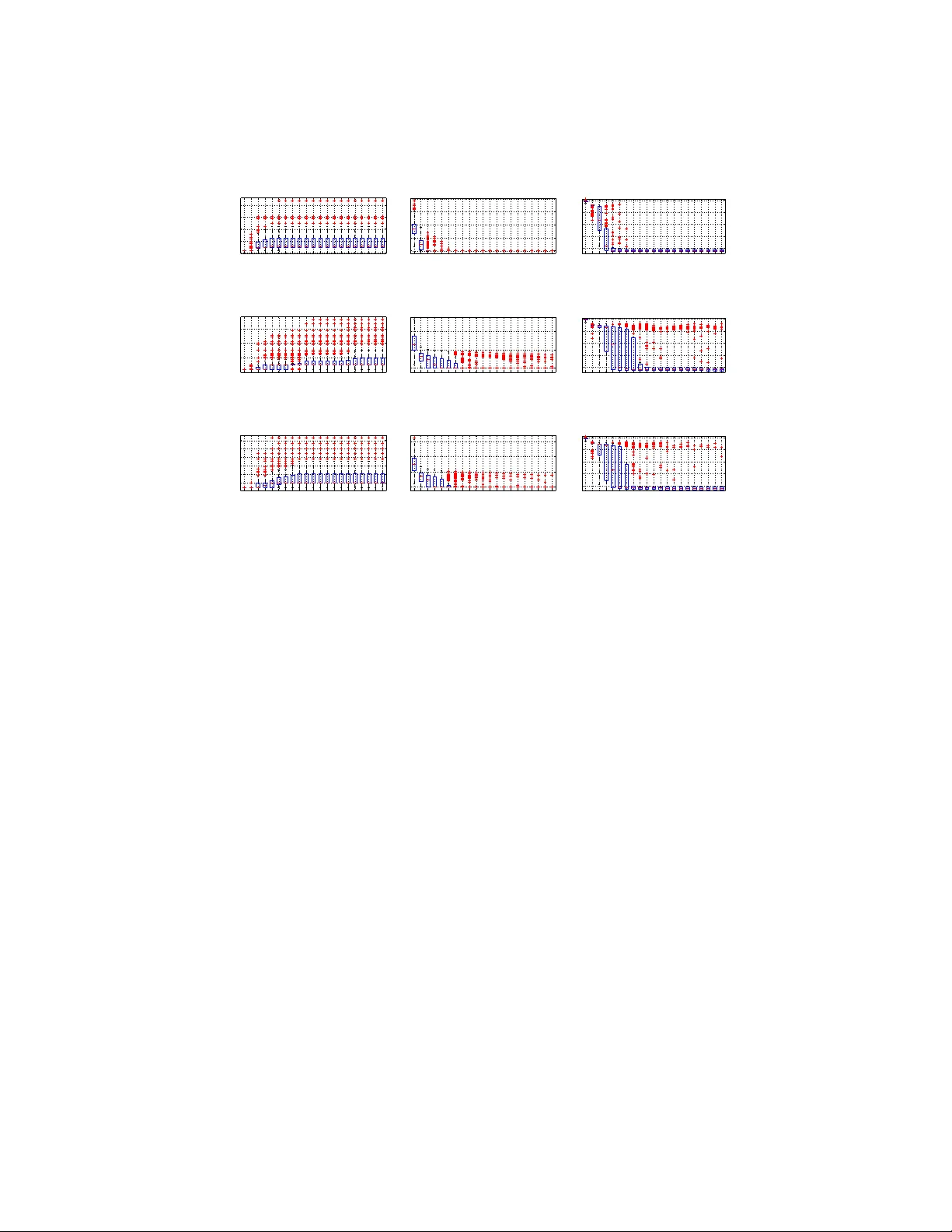
Relaxed Sparse Eigen v alue Conditions for Sparse Estimation via Non-con vex Re gularized Re gression Zheng Pan , Changshui Zhang ∗ Department of Automation, Tsinghua University , Beijing 100084, P .R.China State K ey Lab of Intelligent T ec hnologies and Systems Tsinghua National Laboratory for Information Science and T echnolo gy(TNList) Abstract Non-con ve x regularizers usually impro ve the performance of sparse estimation in prac- tice. T o prov e this fact, we study the conditions of sparse estimations for the sharp concav e regularizers which are a general family of non-con ve x regularizers includ- ing many existing regularizers. For the global solutions of the regularized re gression, our sparse eigen v alue based conditions are weaker than that of L1-regularization for parameter estimation and sparseness estimation. For the approximate global and ap- proximate stationary (AGAS) solutions, almost the same conditions are also enough. W e sho w that the desired A GAS solutions can be obtained by coordinate descent (CD) based methods. Finally , we perform some experiments to show the performance of CD methods on giving A GAS solutions and the degree of weakness of the estimation conditions required by the sharp concav e regularizers. K e ywor ds: Sparse estimation, non-conv ex re gularization, sparse eigen value, coordinate descent 1. Introduction High-dimensional estimation concerns the parameter estimation problems in which the dimensions of parameters are comparable to or larger than the sampling size. In general, high-dimensional estimation is ill-posed. Additional prior knowledge about ∗ Corresponding author Email addr esses: panz09@mails.tsinghua.edu.cn (Zheng P an), zcs@tsinghua.edu.cn (Changshui Zhang) Pr eprint submitted to Elsevier October 9, 2018 the structure of the parameters is usually needed to obtain consistent estimations. In recent years, tremendous research works hav e demonstrated that the prior on sparsity of the true parameters can lead to good estimators, e.g., the well-kno wn work of com- pressed sensing [6] and its extensions to general high-dimensional inference [24]. For high-dimensional sparse estimation, sparsity is usually imposed as sparsity- encouraging [8] regularizers for linear regression methods. Many regularizers have been proposed to describe the prior of sparsity , e.g., ` 0 -norm, ` 1 -norm, ` q -norm with 0 < q < 1 , smoothly clipped absolute deviation (SCAD) penalty [14], log-sum penalty (LSP) [8], minimax concav e penalty (MCP) [37] and Geman penalty (GP) [17, 32]. Except ` 1 -norm, all of these sparsity-encouraging regularizers are non-con ve x. Non- con ve x regularizers were proposed to impro ve the performance of sparse estimation in many applications, e.g., image inpainting and denoising [29], biological feature selec- tion [3, 27], MRI [8, 9, 33, 34, 35] and CT [26, 30]. Howe ver , it still lacks theoreti- cal explanation for the improvement on sparse estimation for non-con ve x regularizers. This paper aims to establish such a theoretical analysis. In the field of sparse estimation, the following three problems are typically studied. In this paper , we mainly study the first two problems. 1. Sparseness estimation: whether the estimation is as sparse as the true parameters; 2. Parameter estimation: whether the estimation is accurate in the sense that the error between the estimation and the true parameter is small under some metric; 3. Feature selection: whether the estimation correctly identities the non-zero com- ponents of the true parameters. For the sparseness estimation, the non-con vex regularizers giv e better approxima- tions to ` 0 -norm than the conv ex ones. They are more probable to encourage the regularized regression to yield sparser estimations than the con vex regularizers. For example, ` q -regularization can give the sparsest consistent estimations ev en when ` 1 - regularization fails [15]. Howe ver , ` q -norm has infinite deriv ati ves at zero and zero vector is al ways a tri vial local minimizer of the regularized regression. The non-con vex regularizers with finite deri vati v es can remedy the numerical problem of ` q -norm, e.g., LSP , SCAD and MCP . These regularizers can also gi v e sparser solutions for more gen- 2 eral situations than ` 1 -regularization in e xperiments [8] and in theory [14, 32, 37, 38]. For the parameter estimation, a lot of applications and experiments have demon- strated that many non-con v ex regularizers gi ve good estimations with far less sampling sizes than ` 1 -norm as the regularizers [8, 9, 26, 30, 33, 34, 35]. In theory , the re- quirements for the sampling sizes are essentially the requirements for design matrix or , rather , estimation conditions . A weaker estimation condition means less sampling size needed or weaker requirements on design matrix. W eaker estimation conditions are important for the application in which the data dimension is very high while the sampling is expensi ve or restrictive. Theoretically , all of the non-conv ex regularizers mentioned above admit accurate parameter estimations under appropriate conditions, e.g., ` q -norm [15], MCP [37], SCAD [37] and general non-con ve x regularizers [38]. There are mainly tw o types of estimation conditions. The first is spar se eigen value (SE) conditions, e.g., the restricted isometry property (RIP) [6, 7] and the SE used by Foucart and Lai [15] and Zhang [40]. The second is restricted eigen value (RE) conditions, e.g., the ` 2 -restricted eigen value ( ` 2 -RE) [2, 21] and restricted in vertibility factor (RIF) [36, 38]. Based on SE, Foucart and Lai [15] gav e a weaker estimation condition for ` q -norm than ` 1 -norm. T rzasko and Manduca [32] established a univ er- sal RIP condition for general non-conv ex regularizers including ` 1 -norm. Since the conditions proposed by Trzasko and Manduca [32] are regularizer -independent, it can not be weakened for non-con ve x regularizers unfortunately . The definition of SE is regularizer -independent while the RE is dependent on the regularizers. RE can giv e a regularizer -dependent estimation condition for general regularizers, e.g., the ` 2 -RE based work by Ne gahban et al. [24] and the RIF based work by Zhang and Zhang [38]. Howe v er , the optimization for non-con vex regularizers is difficult. It usually can- not be guaranteed to achie ve a global optimum for general non-conv ex regularizers. Nev ertheless, some optimization methods can lead to local optimums, e.g., coordi- nate descent [3, 23] and iterativ e reweighted (or majorization-minimization) methods [8, 20, 41, 39], homotopy [37], difference con ve x (DC) methods [27, 28] and proxi- mal methods [18, 25]. Hence, it is meaningful to analyze the performance of sparse estimation for these non-optimal optimization methods. For example, the multi-stage relaxation methods [41, 39] and its one-stage version the adaptiv e LASSO [19, 42] re- 3 place the regularizers with their con ve x relaxations using majorization-minimization. Compared with LASSO, the multi-stage relaxation methods improv e the performance on parameter estimation [39]. Zhang and Zhang [38] use the solutions of LASSO as the initialization and continue to optimize by gradient descent. It is stated that LASSO followed by gradient descent can output an approximate global and stationary solution which is identical to the unique sparse local solution and the global solution. The multi- stage relaxation methods, the ”LASSO + gradient descent” methods and the homotop y methods need the same SE or RE conditions as LASSO. The DC methods [28] and the proximal methods [25] need to know the sparseness of its solutions in advance to ensure the performance of parameter estimation, but these two methods cannot control the sparseness of its solutions explicitly . Based on the related work, we make the follo wing contrib utions: • For a general family of non-con ve x regularizers, we propose new SE based esti- mation conditions which are weaker than that of ` 1 -norm. As far as we kno w , our estimation conditions are the weakest ones for general non-conv ex regularizers. The proposed conditions approach the SE conditions of ` 0 -regularized regres- sion as the regularizers become closer and closer to ` 0 -norm. W e also compare our SE conditions with RE conditions. For ` 1 -regularized regression, RE based estimation conditions are less sev ere than that based on SE [2]. Howe v er , for the case of non-con vex regularizers, their relationship changes. For proper non- con ve x regularizers, SE conditions become weaker than RE conditions, because SE conditions can be greatly weakened from ` 1 -norm to non-con ve x re gularizers while RE conditions remain the same. • Under the proposed SE conditions, we establish upper bounds for the estimation error in ` 2 -norm. The error bounds are on the same order as that of ` 1 -regularized regression. It means that although the proposed SE conditions are weak ened, the parameter estimation performance is not weakened. W ith appropriate additional conditions, we further gi ve the results of sparseness estimations, which sho w the non-con ve x regularized regression give estimations with the sparseness on the same order as the true parameters. 4 • Like the global solutions of non-conv ex regularized regression, we show that the approximate global and approximate stationary (A GAS) solutions [38] also theoretically guarantee accurate parameter estimation and sparseness estimation. The error bounds of parameter estimation are on the order of noise level and the degrees of approximating the stationary solutions and the global optimums. If the degrees of these two approximations are comparable to the noise level, the theoretical performance on parameter estimation and sparseness estimation is also comparable to that of global solutions. Furthermore, the required estima- tion conditions are almost the same as that of global solutions, which means the estimation conditions for A GAS solutions are also weak er than that required by ` 1 -norm. The estimation result on AGAS solutions is useful for application since it shows the robustness of the non-con ve x regularized regression to the inaccuracy of the solutions and gives a theoretical guarantee for the numerical solutions. • Under a mild SE condition, the approximate global (A G) solutions are obtainable and the approximation error is bounded by the prediction error . If the prediction error is small, the solution will be a good approximate global solution. The algo- rithms which control the sparseness of the solutions explicitly are suitable to gi ve good AG solutions, e.g., OMP [31] and GraDeS [16]. For an A G solution, the coordinate descent (CD) methods update it to be approximate stationary (AS) without destroying its A G property . CD have been applied to regularized re- gression with non-conv ex regularizers [3, 23]. Howe ver , the previous works did not allow the non-con v ex regularizers to approximate ` 0 -norm arbitrarily . Our analysis does not hav e such restriction on the non-con ve x regularizers . Denotation. W e use ¯ T to denote the complement of the set T and |T | to denote the number of elements in T . For an index set T ∈ { 1 , 2 , · · · , p } , θ T denotes the restriction of θ = ( θ 1 , θ 2 , · · · , θ p ) on T , i.e., θ T = ( θ i : i ∈ T ) . The support supp ( θ ) of a v ector θ is defined as the index set composed of the non-zero components’ indices of θ , i.e., supp ( θ ) = { i : θ i 6 = 0 } . The ` 0 -norm of the vector θ is the number of non-zero components of θ , i.e., k θ k 0 = | supp ( θ ) | . 5 T able 1: Examples of popular regularizers. The second column is the basis functions of the regularizers. The third column is the zero gaps of the global solutions when the regularizers are ξ -sharp conca ve. The fourth column is the values of λ ∗ . Section 8.2 gi ves the proof for the result on λ ∗ of LSP . Name Basis Functions Zero gap λ ∗ ` 1 -norm r ( u ) = λu 0 λ ∗ = λ ` q -norm r ( u ) = λ 2 ( u/λ ) q , γ = log(1 / (1 − q )) λ ( q (1 − q ) /ξ ) 1 / (2 − q ) λ ∗ = λ (2 − q )  2(1 − q ) ξ  q − 1 2 − q SCAD r ( u ) = λ R u 0 min ( 1 ,  1 − x/λ − 1 γ  + ) dx 0 λ ∗ = λ for ξ = 1 LSP r ( u ) = λ 2 log  1 + u λγ  max { λ (1 / √ ξ − γ ) , 0 } λ ∗ ≤ λ q 2 ξ log(1 + 2 / ( ξγ 2 )) MCP r ( u ) = λ R u 0  1 − x λγ  + dx λ p γ /ξ λ ∗ = λ min { √ γ ξ, 1 } GP r ( u ) = λ 2 u/ ( λγ + u ) max { λ ( 3 p 2 γ /ξ − γ ) , 0 } λ ∗ =    λ ( √ 2 ξ − ξγ / 2) , ξγ 2 ≤ 2 λ/γ , ξγ 2 > 2 2. Preliminaries W e first formulate the sparse estimation problems. Suppose we have n samples ( y 1 , z 1 ) , ( y 2 , z 2 ) , · · · , ( y n , z n ) , where y i ∈ R and z i ∈ R p for i = 1 , · · · , n . Let X = ( z 1 , · · · , z n ) T ∈ R n × p and y = ( y 1 , · · · , y n ) T ∈ R n . W e assume there e xists an s -sparse true parameter θ ∗ which is supported on S and satisfies y = X θ ∗ + e with a small noise e ∈ R n . In this paper , we assume that the energy of the noise is limited by a known le vel  , i.e., k e k 2 ≤  . For Gaussian noise e ∼ N (0 , σ I n ) , this assumption is satisfied for  = σ p n + 2 √ n log n with the probability at least 1 − 1 /n [4]. W e focus on using the following regularized regression to recover θ ∗ from y . This method uses the solutions of the following regularized regression as the estimations to the true parameters. ˆ θ = arg min θ ∈ R p F ( θ ) , (1) where F ( θ ) = L ( θ ) + R ( θ ) . L ( θ ) = k y − X θ k 2 2 / (2 n ) is the pr ediction err or . R ( θ ) is a non-con v ex re gularizer . In this paper , we only study the component-decomposable regularizer , i.e., R ( θ ) = P p i =1 r ( | θ i | ) . W e call r ( u ) the basis function of R ( θ ) . T able 1 lists the basis functions of some popular regularizers. For the basis functions in T able 1, r ( u ) has the formulation r ( u ) = λ 2 r 0 ( u/λ ; γ ) where r 0 ( u ; γ ) is a non-decreasing concav e function ov er [0 , + ∞ ) and γ is a parameter to describe the ”de gree of concav- ity”, i.e., r ( u ) changes from linear function of u to the indicator function I { u 6 =0 } as γ varies from + ∞ to 0 (e xcept ` 1 -norm). Throughout this paper , we assume the basis function r ( u ) satisfy the following 6 properties. All of them hold for the basis functions in T able 1. 1. r (0) = 0 ; 2. r ( u ) is non-decreasing; 3. r ( u ) is conca ve o ver [0 , + ∞ ) ; 4. r ( u ) is continuous and piecewise differentiable. W e use ˙ r ( u +) and ˙ r ( u − ) to denote the right and left deriv ati ves. 5. r ( u ) has the formulation r ( u ) = λ 2 r 0 ( u/λ ; γ ) , where r 0 ( u ; γ ) is parameterized by γ and is independent of λ . In this paper , the weaker SE based estimation conditions need two important prop- erties: zero gap and null consistency [38]. Zero gap means the true parameters and the estimations are strong in the sense that the minimal magnitude of the non-zero components cannot be too close to zero. Null consistency requires that the regularized regression in Eqn. (1) is able to identify the true parameter θ ∗ exactly when θ ∗ = 0 and the error e is inflated by a factor of 1 /η > 1 . Definition 1 (Zero Gap). W e say θ ∈ R p has a zer o gap u 0 for some u 0 ≥ 0 if min {| θ i | : i ∈ supp ( θ ) } ≥ u 0 . Definition 2 (Null Consistency). Let η ∈ (0 , 1) . W e say the r e gularized re gression in Eqn. (1) is η -null consistent if min θ k X θ − e/η k 2 2 / (2 n ) + R ( θ ) = k e/η k 2 2 / (2 n ) . In order to guarantee the above two properties, we propose the following assump- tion, named sharp concavity . Sharp concavity is important for our analysis because zero gap and null consistency can be deri ved from it. Definition 3 (Sharp Conca vity). W e say a basis function r ( u ) satisfies C -sharp con- cavity condition over an interval I if r ( u ) > u ˙ r ( u − ) + C u 2 / 2 holds for any u ∈ I , wher e C is a positive constant. W e also say r ( u ) is C -sharp concave over I and a r e gularizer R ( θ ) is C -sharp concave if its basis function is C -sharp concave. Strictly concave functions can only satisfy r ( u ) > u ˙ r ( u − ) . Howe ver , if the left- deriv ati ve ˙ r ( u − ) decreases so fast that it admits a margin proportional to u 2 in some interval I , the concave functions guarantee the sharp conca vity . 7 C -sharp concavity is satisfied ov er (0 , u 0 ) if r ( u ) is str ongly concave (or − r ( u ) is strongly con ve x) ov er (0 , u 0 ) , i.e., for any t 1 , t 2 ∈ (0 , u 0 ) and α ∈ [0 , 1] , r ( αt 1 + (1 − α ) t 2 ) ≥ α r ( t 1 ) + (1 − α ) r ( t 2 ) + 1 2 C α (1 − α )( t 1 − t 2 ) 2 . (2) Section 8.1 sho ws that sharp concavity only needs Eqn. (2) holds for t 1 = 0 and any t 2 ∈ (0 , u 0 ) , which means that the sharp concavity is weaker than the strong concavity . For example, MCP is ((1 + a ) γ ) − 1 -sharp concav e over (0 , √ 1 + aλγ ) for any a > 0 . Whereas, the strong concavity does not hold ov er ( λγ , √ 1 + aλγ ) . Besides, ` q -norm holds q (1 − q )( u 0 /λ ) q − 2 -sharp concavity over (0 , u 0 ) ; LSP satisfies λ 2 / ( λγ + u 0 ) 2 - sharp concavity o ver (0 , u 0 ) ; GP is 2 λ 3 γ / ( λγ + u 0 ) 3 -sharp concav e ov er (0 , u 0 ) . Let x i be the i-th column of X and ξ = max 1 ≤ i ≤ p k x i k 2 2 /n. W e observe that ξ -sharp concavity deri v es non-trivial zero gaps and null consistenc y . Theorem 1. If r ( u ) is ξ -sharp concave over (0 , u 0 ) , any global solution of Pr oblem (1) has a zer o gap no less than u 0 , i.e., | ˆ θ i | ≥ u 0 for any i ∈ supp( ˆ θ ) . T able 1 lists the zero gaps of ˆ θ when the basis functions are ξ -sharp conca ve. Theorem 2. Let r ( u ) be ξ -sharp concave over (0 , u 0 ) . The η -null consistency condi- tion is satisfied if r ( u 0 ) ≥ 1 2 nη 2 k e k 2 2 . Zhang and Zhang [38] give a probabilistic condition for null consistency when X is drawn from Gaussian distributions. Howe ver , our condition is deterministic from the view of X . It is easy to check whether our condition holds. For the case of r ( u ) = λ 2 r 0 ( u/λ ; γ ) , the condition of Theorem 2 is λ ≥ η − 1 b 0 k e k 2 / √ n , where b 0 = 1 / p 2 r 0 ( u 0 /λ ; γ ) is a constant if u 0 = O ( λ ) (all the regularizers in T able 1 satisfy u 0 = O ( λ ) ). Hence, we assume λ = η − 1 b 0 / √ n (3) in this paper , so that the η -null consistency holds. In addition, we define λ ∗ = inf u> 0 { ξ u/ 2 + r ( u ) /u } . (4) 8 λ ∗ provides a natural normalization of λ [38]. T able 1 lists the values of λ ∗ of the reg- ularizers. W e observe λ ∗ = O ( λ ) from T able 1. In general, for r ( u ) = λ 2 r 0 ( u/λ ; γ ) , we can define a constant a γ (independent to λ ), a γ = inf u> 0 { ξ u/ 2 + r 0 ( u ; γ ) /u } , (5) so that λ ∗ = a γ λ . Thus, we have λ ∗ = η − 1 a γ b 0 / √ n. (6) If the basis function r ( u ) is linear over (0 , u ) for some u > 0 , it is not sharp concav e, e.g., SCAD and truncated ` 1 -norm [39]. W e name such regularizers that are linear near the origin as weak non-con vex re gularizers . The zero gaps of the global solutions with such regularizers cannot be guaranteed to be strictly positi ve. 3. Sparse Estimation of Global Solutions In this section, we show our results on the SE based sparse estimation. Definition 4 (Sparse Eigen value). F or an inte ger t ≥ 1 , we say that κ − ( t ) and κ + ( t ) ar e the minimum and maximum sparse eigen values(SE) of a matrix X if κ − ( t ) ≤ k X ∆ k 2 2 n k ∆ k 2 2 ≤ κ + ( t ) for any ∆ with k ∆ k 0 ≤ t. (7) The SE is related to the restricted isometry constant (RIC) δ t [6, 7], which satisfies 1 − δ t ≤ k X ∆ k 2 2 / ( n k ∆ k 2 2 ) ≤ 1 + δ t for all ∆ with k ∆ k 0 ≤ t . Thus, it follows that δ t = ( κ + ( t ) − κ − ( t )) / ( κ + ( t ) + κ − ( t )) , where δ t is actually the RIC of the scaled matrix 2 X/ ( κ + ( t ) + κ − ( t )) . W e employ SE since it allo ws κ + ( t ) ≥ 2 and av oids the scaling problem of RIC [15]. In order to show the typical values of κ + ( t ) and κ − ( t ) , we compute them and their ratio κ + ( t ) /κ − ( t ) for the standard Gaussian n × p matrix 1 , where we fix p = 10 000 , n = 500 , 1000 , 1500 , 2000 and t varies from 1 to n . It should be noted 1 The elements are i.i.d. drawn from the standard Gaussian distrib ution N (0 , 1) . 9 0 500 1000 1500 1 1.5 2 2.5 3 3.5 4 t ˜ κ + ( t ) n=500 n=1000 n=1500 n=2000 (a) 0 500 1000 1500 10 −6 10 −4 10 −2 10 0 t ˜ κ − ( t ) n=500 n=1000 n=1500 n=2000 (b) 0 200 400 600 800 1000 1200 1400 10 0 10 2 10 4 10 6 t ˜ κ + ( t ) / ˜ κ − ( t ) n=500 n=1000 n=1500 n=2000 (c) Figure 1: ˜ κ + ( t ) , ˜ κ − ( t ) and ˜ κ + ( t ) / ˜ κ − ( t ) for the Gaussian random matrices with p = 10 000 , n = 500 , 1000 , 1500 , 2000 and t ranges from 1 to n . The solid lines are the av erage values of the 100 trials and the two dash lines around each solid line are the maximum and the minimum of the 100 trials. that κ + ( t ) and κ − ( t ) cannot be obtained efficiently . W e use the following approx- imation method: For a matrix X ∈ R n × p , we randomly sample its 100 submatri- ces X 1 , X 2 , · · · , X 100 ∈ R n × t composed by t columns of X and regard ˜ κ + ( t ) = max i λ max ( X T i X i ) and ˜ κ − ( t ) = min i λ min ( X T i X i ) as the approximations for κ + ( t ) and κ − ( t ) , where λ max ( A ) and λ min ( A ) mean the maximal and minimal eigen v alues of A . Actually , ˜ κ + ( t ) ≤ κ + ( t ) and ˜ κ − ( t ) ≥ κ − ( t ) . For each n and t , we generate 100 standard Gaussian matrices and compute the maximums, minimums and the means of the values of ˜ κ + ( t ) , ˜ κ − ( t ) and ˜ κ + ( t ) / ˜ κ − ( t ) for the 100 trials. Figure 1 illustrates the results. The variances of ˜ κ + ( t ) , ˜ κ − ( t ) and ˜ κ + ( t ) / ˜ κ − ( t ) with the same n and t are small since the corresponding lines for the maximum, minimum and mean values are close to each other . Howe ver , ˜ κ + ( t ) / ˜ κ − ( t ) gro ws very fast as t grows or n decreases. Based on SE, we establish the following parameter estimation result for global solutions of non-conv ex regularized regression. Let ˆ ρ 0 and ρ ∗ 0 be the zero gaps of the global solution ˆ θ and the true parameter θ ∗ respectiv ely . Denote ρ 0 = min { ˆ ρ 0 , ρ ∗ } . (8) Theorem 3 (P arameter Estimation of Global Solutions). Suppose the following con- ditions hold. 1. r ( u ) is invertible for u ≥ 0 and r − 1 ( u/s 1 ) /r − 1 ( u/s 2 ) is a non-decreasing function of u for any s 2 ≥ s 1 ≥ 1 ; 2. The r e gularized r e gr ession satisfies η -null consistency; 10 3. The following SE condition holds for some inte ger t ≥ αs , κ + (2 t ) /κ − (2 t ) < 4( √ 2 − 1) H r ( ρ 0 , α , s, t ) + 1 , (9) wher e s = k θ ∗ k 0 , α = 1+ η 1 − η , H r ( ρ 0 , α , s, t ) = p s t r − 1 ( r ( ρ 0 ) /s ) r − 1 ( αr ( ρ 0 ) /t ) for ρ 0 > 0 and H r (0 , α , s, t ) = lim ρ → 0+ H r ( ρ, α , s, t ) . Then, k ˆ θ − θ ∗ k 2 ≤ C 1 λ ∗ , (10) wher e C 1 = (1+ √ 2)(1+ η ) √ t κ − (2 t ) H r ( ρ 0 ,α,s,t )+1 / 2 H r ( ρ 0 ,α,s,t ) − (1+ √ 2)( κ + (2 t ) /κ − (2 t ) − 1) / 4 . Since λ ∗ is on the order of noise lev el  (Eqn. (6)), the estimation error k ˆ θ − θ ∗ k 2 is at most on the order of noise lev el. W e giv e a detailed discussion on Theorem 3 in Section 4. Before the discussion, we first show a corollary given in Section 4, which shows that our SE condition only needs κ − ( t ) > 0 with t = O ( s ) . This SE condition is much weaker than that of ` 1 -norm. In fact, it is almost optimal since it is the same as the estimation condition of ` 0 -regularization [15, 38]. Corollary 1. Let the condition 1 and 2 of Theor em 3 hold and H r ( ρ 0 , α , s, αs + 1) → ∞ as γ → 0 . If κ − (2 αs + 2) > 0 , ther e exists γ > 0 suc h that k ˆ θ − θ ∗ k 2 ≤ O ( λ ∗ ) . In addition to the error bound in Theorem 3, we hope that the regularized regres- sions yield enough sparse solutions. W e extend the results from Zhang and Zhang [38] and show that the global solutions are sparse under appropriate conditions. Theorem 4 (Sparseness Estimation of Global Solutions). Suppose the conditions of Theor em 3 hold. Consider l 0 > 0 and inte ger m 0 > 0 such that p 2 tκ + ( m 0 ) r ( C 2 (1 + η ) λ ∗ ) /m 0 + k X T e/n k ∞ < ˙ r ( l 0 − ) , wher e C 2 is defined in Eqn. (31). Then, | supp ( ˆ θ ) \S | ≤ m 0 + tr ( C 2 (1 + η ) λ ∗ ) /r ( l 0 ) . Corollary 2. Suppose the basis function r ( u ) = λ 2 r 0 ( u/λ ) and the conditions of The- or em 4 hold with t = ( α + 1) s , m 0 = β 0 s and l 0 = β 1 λ for some β 0 , β 1 > 0 . Let 11 C 3 = C 2 (1 + η ) a γ wher e C 2 is the same as Theor em 4 and a γ is defined in Eqn. (5). If 2( α + 1) κ + ( β 0 s ) β 0 < ( ˙ r 0 ( β 1 − ) − η a γ ) 2 r 0 ( C 3 ) , (11) then | supp ( ˆ θ ) \S | ≤ ( β 0 + ( α + 1) r 0 ( C 3 ) /r 0 ( β 1 )) s. (12) Example for Corollary 2. Consider the example of LSP with r 0 ( u ) = log(1 + u/γ ) and β 1 = √ γ . Suppose the columns of X are normalized so that ξ = 1 . Section 8.2 sho ws that a γ ≤ p 2 log (1 + 2 /γ 2 ) . Thus, the right hand of Eqn (11) is lar ger than  1 / (1 + √ γ ) − η p 2 γ log(1 + 2 /γ 2 )  2 γ log(1 + γ − 1 C 2 (1 + η ) p 2 log (1 + 2 /γ 2 )) Thus, as γ goes to 0, the right side of Eqn. (11) is arbitrarily large. Eqn. (11) holds for enough small γ . The right side of Eqn. (12) is β 0 s + O ( s ) as γ → 0 . Hence, we can freely select β 0 satisfying Eqn. (11) with enough small γ . For example, if β 0 = 1 /s , Eqn. (11) holds for enough small γ and Eqn. (12) becomes | supp ( ˆ θ ) / S | ≤ 1 + s ( α + 1) log(1 + γ − 1 C 2 (1 + η ) p 2 log (1 + 2 /γ 2 )) log(1 + 1 / √ γ ) . (13) The right side of Eqn (13) is at most on the order of s when γ is close to zero. 4. Discussion on Theorem 3 This section giv es some detailed discussion on Theorem 3. 4.1. In vertible appr oximate r e gularizer s If r ( u ) is not inv ertible, e.g., MCP , we can design inv ertible basis function to ap- proximate it. For example, we can use the following inv ertible function, named Ap- pr oximate MCP , to approximate MCP . r ( u ) =    λu − u 2 / (2 γ ) , 0 ≤ u ≤ λγ (1 − φ ) , 1 2 λ 2 γ (1 − φ 2 )  u λγ (1 − φ )  2 φ/ (1+ φ ) , u > λγ (1 − φ ) , (14) where φ ∈ (0 , 1) . Approximate MCP is concatenated by the part of MCP over [0 , λγ (1 − φ )] and the part of ` q -norm ov er ( λγ (1 − φ ) , ∞ ) with q = 2 φ/ (1 + φ ) . When φ → 0 , 12 r ( u ) will become the basis function of MCP . W e will address the method to obtain Eqn. (14) in Section 8.7. Any other non-in vertible regularizers in T able 1 can be approxi- mated in the same way . 4.2. Non-decr easing pr operty of r − 1 ( u/s 1 ) /r − 1 ( u/s 2 ) It can be verified that all the regularizers in T able 1 or their in vertible approximate ones (in the way of Eqn. (14)) satisfy the non-decreasing property of r − 1 ( u/s 1 ) r − 1 ( u/s 2 ) for an y s 2 ≥ s 1 > 0 . In fact, for deriv ativ e basis functions, this non-decreasing property is equal to that u ˙ r ( u ) /r ( u ) is a non-increasing function of u . 4.3. Non-sharp concave r e gularizers If r ( u ) is not ξ -sharp concave, e.g., SCAD or LSP with γ 2 > 1 /ξ , we cannot guarantee ˆ θ has a positiv e zero gap. In this case, the condition 2 (null consistency) of Theorem 3 can be guaranteed by the ` 2 -regularity conditions [38] and the condition 3 becomes κ + (2 αs ) /κ − (2 αs ) < 1 . 65 / √ α + 1 with t = αs , which also belongs to the ` 2 -regularity conditions. Hence, without ξ -sharp conca vity , Theorem 3 still holds. Intuitiv ely , non-sharp concave regularizers need the same estimation conditions as ` 1 - regularization since the y cannot approximate ` 0 -norm arbitrarily . 4.4. Relaxed SE based estimation conditions Much more relaxed estimation conditions are sufficient for ξ -sharp concave regu- larizers. Suppose r ( u ) is ξ -sharp concav e over (0 , ρ 0 ) with 0 < ρ 0 ≤ min i ∈S | θ ∗ i | . In this case, H r ( ρ 0 , α , s, t ) can become arbitrarily large for proper regularizers so that the SE condition in Eqn. (9) is much weaker than the SE conditions of ` 1 -regularized regression. W e hav e shown in Figure 1 that ˜ κ + ( t ) / ˜ κ − ( t ) ( ≤ κ + ( t ) /κ − ( t ) ) increases very fast as t increases or n decreases. Thus, a weak er constraint on κ + (2 t ) /κ − (2 t ) in Eqn. (9) is very important for sparse estimation problems. Here, we give the examples of approximate MCP , ` q -norm and LSP . For approxi- mate MCP , Eqn. (15) gives its H r ( ρ 0 , α , s, t ) (see Section 8.7). H r ( ρ 0 , α , s, t ) = α − 1 / 2 ( t/ ( αs )) 1 2 φ , (15) 13 10 −20 10 −15 10 −10 10 −5 10 0 0 5 10 15 20 25 30 γ 4( √ 2 − 1) H r + 1 AMCP s=5 AMCP s=10 AMCP s=50 AMCP s=100 L1 (a) Approximate MCP vs. L1 10 −3 10 −2 10 −1 10 0 0 5 10 15 20 25 30 Γ = 1 / log(1 / γ ) 4( √ 2 − 1) H r + 1 LSP s=5 LSP s=10 LSP s=50 LSP s=100 L1 (b) LSP vs. L1 10 −1 10 0 0 5 10 15 20 25 30 γ = log(1 / (1 − q )) 4( √ 2 − 1) H r + 1 Lq L1 (c) ` q -norm vs. L1 Figure 2: The upper bounds of the SE conditions for LSP , approximate MCP(AMCP) and ` q -norm. W e set α = 1 . 01 , t = 2 s . In each subfigure, we also plot the upper bound of SE conditions for ` 1 -norm, i.e., the right hand of Eqn. (16) with q = 1 . where we set γ ξ = φ 1+ φ ( α/t ) 1 /φ . For ` q -norm, the SE conditions can be written as κ + (2 t ) κ − (2 t ) < 1 + 4( √ 2 − 1) √ α  t αs  1 /q − 1 / 2 . (16) When α = 1 , Eqn. (16) is identical to the estimation condition of F oucart and Lai [15]. Hence, Foucart and Lai [15] can be regarded as a special case of our theory . For LSP , we hav e H r ( ρ 0 , α , s, t ) = r s t (1 + ρ 0 / ( λγ )) 1 s − 1 (1 + ρ 0 / ( λγ )) α t − 1 = r s t ( γ √ ξ ) − 1 /s − 1 ( γ √ ξ ) − α/t − 1 . (17) It should be noted that H r ( ρ 0 , α , s, t ) → ∞ as γ → 0 for approximate MCP , ` q - norm and LSP . Figure 2 shows some special cases of H r ( ρ 0 , α , s, t ) for these three regularizers and ` 1 -norm. In Figure 2, the SE conditions in Eqn. (9) are much weaker than that of ` 1 -norm. Theorem 3 rev eals that the upper bound constraint for κ + (2 t ) /κ − (2 t ) tends to infinity as γ → 0 for proper non-con vex re gularizers. It implies that if κ − (2 t ) = inf θ  k X ∆ k 2 2 n k ∆ k 2 2 : k ∆ k 0 ≤ 2 t  > 0 , (18) there exists γ > 0 so that the SE condition (Eqn. (9)) is satisfied. Based on this observation, we have Corollary 1. In Corollary 1, κ − (2 αs + 2) > 0 holds if the columns of X are in general position 2 and 2 αs + 2 ≤ n , which is almost optimal in 2 General position means any n columns of X are linear independent. The columns of X are in general position with probability 1 if the elements of X are i.i.d. drawn from some distrib ution, e.g., Gaussian. 14 the sense that it is the same as the SE condition of ` 0 -regularized re gression [38]. 4.5. Comparison between SE and RE Like SE, RE is also popular to construct estimation conditions. There are some variants of RE, e.g., ` 2 -RE [2, 21] and RIF [36, 38]. It can derive a simple expression to the parameter estimation and the corresponding estimation condition. Definition 5 ( ` 2 -RE). F or α ≥ 1 , a r e gularizer R , an index set S ⊂ { 1 , · · · p } and its complement set ¯ S , the ` 2 -RE is defined as RE R ( α, S ) = inf ∆  k X ∆ k 2 2 n k ∆ k 2 2 : R (∆ ¯ S ) ≤ α R (∆ S )  . (19) Definition 6 (Restricted In vertibility F actor). F or τ ≥ 1 , α ≥ 1 , a r e gularizer R , an index set S ⊂ { 1 , · · · p } , RIF is defined as RIF R τ ( α, S ) = inf ∆  |S | 1 /τ k X T X ∆ k ∞ n k ∆ k τ : R (∆ ¯ S ) ≤ α R (∆ S )  . Theorem 5. Suppose η -null consistency condition holds and α = (1 + η ) / (1 − η ) . Then, k ˆ θ − θ ∗ k 2 ≤ 2 α √ s RE R ( α, S ) ˙ r (0+) . F or any τ ≥ 1 , k ˆ θ − θ ∗ k τ ≤ (1+ η ) λ ∗ s 1 /τ RIF R τ ( α, S ) . The estimation conditions based on RE require that RE R ( α, S ) > 0 or RIF R τ ( α, S ) > 0 . The same conclusion also can be obtained for ` 1 -regularized regression [24, 38]. What we are interested in is whether non-con ve x regularizers allow a larger value of RE R ( α, S ) than ` 1 -norm, i.e., whether RE R ( α, S ) > 0 becomes weaker by employing non-con ve x regularizers. Define Ω( β ) = { ∆ ∈ R n : R ( β ∆ ¯ S ) ≤ α R ( β ∆ S ) , k ∆ k 2 = 1 } for β > 0 . The concavity of r ( u ) gi ves that ˙ r (0+) u ≥ r ( u ) ≥ u ˙ r ( u − ) , which deri ves that Ω( β ) ⊃ { ∆ ∈ R n : ˙ r (0+) β k ∆ ¯ S k 1 ≤ α β h| ∆ S | , ˙ r ( | β ∆ S |− ) i , k ∆ k 2 = 1 } , where | ∆ S | is the vector composed of the absolute values of the components of ∆ S , i.e., | ∆ S | = ( | ∆ i | : i ∈ S ) . In the same way , ˙ r ( | β ∆ S |− ) = ( ˙ r ( | β ∆ i |− ) : i ∈ S ) . 15 Thus, we giv e an upper bound to RE R ( α, S ) : RE R ( α, S ) = inf β > 0 , ∆ ∈ R p { k X ∆ k 2 2 n k ∆ k 2 2 : ∆ ∈ Ω( β ) } ≤ inf β > 0 , ∆ ∈ R p { k X ∆ k 2 2 n k ∆ k 2 2 : ˙ r (0+) k ∆ ¯ S k 1 ≤ α h| ∆ S | , ˙ r ( | β ∆ S |− ) i , k ∆ k 2 = 1 } ( β → 0+) ≤ inf ∆ ∈ R p { k X ∆ k 2 2 n k ∆ k 2 2 : k ∆ ¯ S k 1 ≤ α k ∆ S k 1 , k ∆ k 2 = 1 } = RE ` 1 ( α, S ) RE R ( α, S ) ≤ RE ` 1 ( α, S ) means that the RE based condition of non-con vex reg- ularized regression RE R ( α, S ) > 0 is not relaxed. Negahban et al. [24] put an ad- ditional constraint U (  ) = { ∆ : k ∆ k ≥  } to the definition of RE. This constraint av oids the bad case ∆ → 0 . Howe ver , it still cannot guarantee to provide larger RE for non-con ve x regularizers than ` 1 -norm. For example, let t 1 , t 2 and t 3 sat- isfy that | t 1 | + | t 2 | ≤ 2 | t 3 | and α = 2 , S = { 3 } and ¯ S = { 1 , 2 } . Thus, the concavity of r ( u ) implies that r ( | t 1 | ) + r ( | t 2 | ) ≤ 2 r (( | t 1 | + | t 2 | ) / 2) ≤ 2 r ( | t 3 | ) . For this case, { ∆ : k ∆ ¯ S k 1 ≤ α k ∆ S k 1 } ⊂ { ∆ : R (∆ ¯ S ) ≤ α R (∆ S ) } . Thus, RE R ( α, S ) ≤ RE ` 1 ( α, S ) . For RIF , we hav e the same result. Although non-con ve x regularizers gi ve better approximations to ` 0 -norm, the RE of non-con v ex regularizers cannot be guaranteed to be lager than that of ` 1 -norm. The framework of RE does not leav e space to relax the estimation condition for non-con ve x regularizers. The only difference between the definitions of SE and RE lies in the constraints for ∆ . The two constraints { ∆ : k ∆ k 0 ≤ 2 t } and { ∆ : R (∆ ¯ S ) ≤ α R (∆ S ) do not contain each other . Howe ver , we observe that κ − (2 t ) ≥ min |T |≤ s RE R ((2 t − s ) /s, T ) ≥ min |T |≤ s RE R (2 α − 1 + 2 /s, T ) for t ≥ αs + 1 . When η is small and s  2 , 2 α − 1+ 2 /s is close to α and min |T |≤ s RE R (2 α − 1+ 2 /s, T ) ≈ min |T |≤ s RE R ( α, T ) . Hence, with proper regularizers, the SE condition in Eqn. (18) is a weaker condition than min |T |≤ s RE R ( α, T ) > 0 . W e can also compare RE and our SE conditions with the help of the failure bound of RIC δ 2 s = 1 / √ 2 for ` 1 -minimization recov ery [12], where ` 1 -minimization re- cov ery includes the basis pursuit [10] and Dantzig selector [5]. The failure bound means that for any ε > 0 there exists X ∈ R ( p − 1) × p with δ 2 s < 1 / √ 2 + ε where 16 ` 1 -minimization recovery fails. On the other hand, ` 1 -minimization recovery suc- ceeds when RE ` 1 ( α, S ) > 0 [2], like ` 1 -regularized regression (Theorem 5). Thus, min |T |≤ s RE ` 1 ( α, T ) = 0 if δ 2 s ≥ 1 / √ 2 , i.e., κ + (2 s ) /κ − (2 s ) ≥ 3 + 2 √ 2 . Since non-con ve x regularizers cannot weaken RE conditions, κ + (2 s ) /κ − (2 s ) ≥ 3 + 2 √ 2 also causes min |T |≤ s RE R ( α, T ) = 0 for non-conv ex regularizers. On the contrary , our SE conditions, e.g., κ − (2 αs + 2) > 0 , still hold with proper non-con ve x regulariz- ers ev en when κ + (2 s ) /κ − (2 s ) ≥ 3 + 2 √ 2 . 4.6. Comparison with the conditions for featur e selection Shen et al. [28] gav e a necessary condition for consistent feature selection, which can be relaxed further to κ − ( s ) > C log p/n with a constant C > 0 independent of p, s, n . This necessary condition needs κ + ( s ) /κ − ( s ) to be upper bounded by a constant which is independent of the regularizers. For their DC algorithm based methods, they tightened the conditions to that κ + (2 ˜ s ) /κ − (2 ˜ s ) is upper bounded, where ˜ s is the number of non-zero components of the solutions gi ven by their methods. This condition cannot be verified until the solutions are given. Howe ver , our SE conditions do not depend on the sparseness of the practical solutions (see Section 5). 5. Sparse Estimation of A GAS Solutions For Problem (1), it is practical to obtain a solution which is approximate global (A G) (Definition 7) and approximate stationary (AS) (Definition 8). W e show in this section that this kind of solutions also giv e good estimation to the true parameters. Definition 7. Given µ ≥ 0 , we say ˜ θ is a ( θ ∗ , µ ) -approximate global solution of min θ F ( θ ) if F ( ˜ θ ) ≤ F ( θ ∗ ) + µ . Definition 8. Given ν ≥ 0 , we say ˜ θ is a ν -approximate stationary solution of min θ F ( θ ) if the dir ectional derivative of F at ˜ θ in any dir ection d ∈ R p with k d k 2 = 1 is no less than − ν , i.e ., F 0 ( θ ; d ) ≥ − ν . The directional deriv ati ve is defined as F 0 ( θ ; d ) = lim inf λ ↓ 0 ( F ( θ + λd ) − F ( θ )) /λ for any θ ∈ R p and d ∈ R p . For Problem (1), F 0 ( θ ; d ) = d T ∇L ( θ ) + P p i =1 R 0 ( θ i ; d i ) . 17 The follo wing theorem gi ves the parameter estimation result with A GAS solutions. Let ˜ u 0 ≥ 0 be the zero gap of ˜ θ and ˜ ρ 0 = min { ˜ u 0 , min i ∈ supp ( θ ∗ ) | θ ∗ i |} . Theorem 6 (P arameter Estimation of A GAS solutions). Suppose the following con- ditions hold for the r e gularized r e gr ession. 1. ˜ θ is a ( θ ∗ , µ ) -AG solution and ν -AS solution. 2. r ( u ) is invertible for u ≥ 0 and r − 1 ( u/s 1 ) /r − 1 ( u/s 2 ) is a non-decreasing function w .r .t. u for any s 2 ≥ s 1 > 0 ; 3. The r e gularized r e gr ession satisfies η -null consistency; 4. The following SE condition holds for some inte ger t ≥ αs + 1 , κ + (2 t ) /κ − (2 t ) < 4( √ 2 − 1) G r ( ˜ ρ 0 , α , s, t ) + 1 , (20) wher e α = 1+ η 1 − η , G r ( ˜ ρ 0 , α , s, t ) = √ st t − 1 r − 1 ( r ( ˜ ρ 0 ) /s ) r − 1 ( αr ( ˜ ρ 0 ) / ( t − 1)) for ˜ ρ 0 > 0 and G r (0 , α, s, t ) = lim ρ → 0+ G r ( ρ, α , s, t ) . Then, k ˜ θ − θ ∗ k 2 ≤ C 4 ˜  + C 5 r − 1 ( µ 1 − η ) , wher e ˜  = ˙ r (0+) + η λ ∗ + ν and C 4 , C 5 ar e positive constants. C 4 and C 5 ar e defined in Eqn. (39) and (40). The condition 2, 3 and 4 are almost the same as the three conditions of Theorem 3 except the slightly different requirements for t and the definition of G r ( ˜ ρ 0 , α , s, t ) . Consequently , the discussion in Section 4 is also suitable for this theorem: 1. The non-in vertible basis functions can be approximated by approximate inv ert- ible basis functions; 2. W ithout ξ -sharp concavity , the condition 4 of Theorem 6 is almost the same as RIP conditions in Foucart and Lai [15]; 3. W ith ξ -sharp concavity and a positive zero gap (we sho w in Theorem 9 that our CD methods guarantee the positive zero gaps), SE based estimation conditions can be much relaxed. Theorem 6 shows that the error bounds of parameter estimation are mainly deter- mined by four parts: the slope of r ( u ) at zero ˙ r (0+) , the parameter λ ∗ = O ( / √ n ) , the degree of approximating the stationary solutions ν and the degree of approximating 18 the global optimums r − 1 ( µ/ (1 − η )) . If r ( u ) = λ 2 r 0 ( u/λ ; γ ) and r 0 ( u ; γ ) has a finite deriv ati ve at zero, we kno w that ˙ r (0+) = λ ˙ r 0 (0+; γ ) , e.g., ˙ r (0+) = λ for MCP . Since λ = O ( / √ n ) by Eqn. (3) in this paper, the estimation error bound is actually k ˜ θ − θ ∗ k 2 ≤ O ( / √ n ) + O ( ν ) + O ( r − 1 ( µ/ (1 − η ))) . According to Theorem 6, we do not need to solve Problem (1) exactly . A good sub- optimal solution is enough to giv e good parameter estimation. Even, we do not need a strictly stationary solution since Theorem 6 allows a margin ν . So, the non-con vex regularized regression is robust to the inaccuracy of the solutions, which is important for numerical computation. It should be noted that ˙ r (0+) is required to be finite in Theorem 6, which forbids the regularizers with infinite ˙ r (0+) , e.g., ` 0 -norm and ` q -norm ( 0 < q < 1 ). It may be due to the strongly NP-hard property brought by ` 0 -norm and ` q -norm regularized regression [11]. Similar to Theorem 4, we give the following sparseness estimation result for A GAS solutions. The proof is the same as that of Theorem 4. Theorem 7 (Sparseness Estimation of A GAS solutions). Suppose the conditions of Theor em 6 hold. Let b = ( t − 1) r  c 4 ˜  + c 5 r − 1  µ 1 − η  , wher e c 4 and c 5 ar e defined in Eqn. (37) and Eqn. (38). Consider l 0 > 0 and inte ger m 0 > 0 such that s 2 κ + ( m 0 ) m 0 ( µ 1 − η + b ) + k X T e/n k ∞ ≤ ˙ r ( l 0 − ) . Then, | supp ( ˜ θ ) \S | < m 0 + b/r ( l 0 ) . The sparseness of A GAS solutions is also af fected by ˜  = ˙ r (0+) + η λ ∗ + ν and µ . Theorem 7 can also deriv e a similar conclusion as Corollary 2. For an AGAS solution with small ν and µ , the sparseness of the solution is on the order of s , just like the global solutions. 5.1. Appr oximate Global Solutions W e need AG solutions in Theorem 6 and Theorem 7. The methods to obtain such solutions are crucial consequently . Instead of restricting to the solutions giv en by a 19 specific algorithm, we use the prediction error k X θ 0 − y k 2 2 / (2 n ) to give a quality guarantee for any solution θ 0 that is regarded as an A G solution. Theorem 8. Suppose θ 0 is an s 0 -sparse vector with the pr ediction err or µ 2 0 = k X θ 0 − y k 2 2 / (2 n ) . If κ − ( s + s 0 ) > 0 , then θ 0 is a ( θ ∗ , µ )-A G solution wher e µ = µ 2 0 + ( s + s 0 ) r √ 2 µ 0 + / √ n p ( s + s 0 ) κ − ( s + s 0 ) ! Corollary 3. Suppose θ 0 is an s 0 -sparse vector with the pr ediction err or µ 0 = ζ / √ n for some ζ ≥ 0 and the basis function has the formulation r ( u ) = λ 2 r 0 ( u/λ ) with λ = η − 1 b 0 / √ n . Then, θ 0 is a ( θ ∗ , C 6  2 /n ) -A G solution wher e C 6 = ζ 2 + ( s + s 0 ) b 2 0 η 2 r 0 (1 + √ 2 ζ ) η b 0 p ( s + s 0 ) κ − ( s + s 0 ) ! . The methods that explicitly control the sparseness of its solutions are suitable for giving the AG solutions, e.g., OMP [31] and GraDeS [16]. Howe ver , we do not need the strong conditions for consistent parameter estimation for these methods, e.g., δ 2 s < 1 / 3 for GraDeS [16] or ( κ + (1) /κ − ( t )) log ( κ + ( s ) /κ − ( t )) gro ws sub-linearly as t for OMP [40]. In fact, Theorem 8 only requires κ − ( s + s 0 ) > 0 . Hence, s 0 can be large enough to make µ 0 to be small. The relationship between µ 0 and s 0 depends on the employed method and the design matrix X . Even with a bad value of µ in the initialization, we can decrease it further by CD methods as stated in Section 5.2. 5.2. Appr oximate Stationary Solutions with Zer o Gap Theorem 6 also requires the solution to be ν -AS and has a positiv e zero gap. Gen- eral gradient descent algorithms can pro vide stationary solutions but they cannot ensure a positiv e zero gap. Howe v er , we observe that the coordinate descent (CD) methods can yield AS solutions and all of these solutions ha ve positive zero gaps under proper sharp concavity conditions. In ev ery step, CD only optimizes for one dimension, i.e., θ ( k ) i = arg min u ∈ R F (( θ ( k ) 1 , · · · , θ ( k ) i − 1 , u, θ ( k − 1) i +1 , · · · , θ ( k − 1) p ) T ) + ψ 2 ( u − θ ( k − 1) i ) 2 , (21) 20 where k is the number of iterations, i = 1 , · · · , p and ψ > 0 is a positi ve constant. The constant ψ plays a role of balance between decreasing F ( θ ) and not going f ar from the previous step. The above CD method is also called pr oximal coordinate descent . For Problem (1), the CD methods iterate as follows. θ ( k ) i = arg min u ∈ R 1 2  k x i k 2 2 n + ψ  u − ψ θ ( k − 1) i + x T i ω ( k ) i /n ψ + k x i k 2 2 /n ! 2 + r ( | u | ) , (22) where x i is the i-th column of the design matrix X and ω ( k ) i = y − P j i x j θ ( k − 1) j . Problem (22) is a non-conv ex b ut only one-dimensional problem. All of its solutions are between 0 and ψ θ ( k − 1) i + x T i ω ( k ) i /n ψ + k x i k 2 2 /n . W e assume that Problem (22) can be exactly solved. If Problem (22) has more than one minimizer, any one of them can be selected as θ ( k ) i . In this paper, CD methods stop iterating if k θ ( k ) − θ ( k − 1) k 2 ≤ τ , (23) where τ > 0 is a small tolerance proportional to the v alue ν (see Theorem 10). Theorem 9. If r ( u ) is ( ξ + ψ ) -sharp concave o ver (0 , u 0 ) , then θ ( k ) i ≥ u 0 or θ ( k ) i = 0 for any k = 1 , 2 , · · · and any i = 1 , · · · , p . The above zero gap property of CD is a corollary of Theorem 1. The sharp con- cavity condition of Theorem 9 is a little stronger than the requirements of Theorem 3. Nonetheless, we can set ψ to be small to narrow the difference between the sharp concavity conditions of Theorem 3 and Theorem 9. Besides the zero gap, we show in the following theorem that CD methods simulta- neously giv e AS solutions and keep them to be still A G solutions. Theorem 10. {F ( θ ( k ) ) } is a non-increasing sequence and con ver ges; F or any ν > 0 and with τ = ν / ( √ p ( ψ + pξ )) , CD stops within k = 1 + 2 p ( ψ + pξ ) 2 F ( θ (0) ) ψ ν 2 iterations and outputs a ν -AS solution, wher e p is the number of columns of the design matrix X . Theorem 10 sho ws CD methods gi ve a further decrease to the value µ of A G prop- erty and guarantees the ν -AS property , which is necessary for sparse estimation in Theorem 6 and Theorem 7. This theorem also gives an upper bound for ν , i.e., ν ≤ √ p ( ψ + pξ ) k θ ( k ) − θ ( k − 1) k 2 , (24) 21 where k is the number of iterations. Usually , we hope ν is on the order of λ ∗ so that ˜  = ˙ r (0+) + η λ ∗ + ν = O ( λ ∗ ) = O ( / √ n ) in Theorem 6. CD has been applied to the non-conv ex regularized regression by Breheny and Huang [3] and Mazumder et al. [23] . Howe ver , their non-con vex regularizers are restrictiv e because they need Eqn. (22) to be strictly conv ex for ψ = 0 . They could not deal with the MCP with γ ≤ 1 , the SCAD with γ ≤ 2 or the LSP with γ ≤ 1 . Compared with them, the conclusions of Theorem 10 are weaker but they are enough to obtain ν -AS solutions and the re gularizers can approximate ` 0 -norm arbitrarily . 6. Experiment In this section, we experimentally sho w the performance of CD methods on gi ving A GAS solutions and the degree of weakness of the estimation conditions required by the sharp concav e regularizers. 6.1. A GAS solutions In Section 5, we pro ve that µ is monotonously decreasing, ν tends to 0 and the zero gap ˜ u 0 is maintained in each iteration of CD algorithm. W e experimentally sho w these in this part. W e set the dimension of the parameter as p = 1000 , the number of non-zero com- ponents of θ ∗ (the true parameter) s = log p . W e randomly choose s indices as the non-zero components. The non-zero components are i.i.d. drawn from N (0 , 1) and those belonging to ( − 0 . 1 , 0 . 1) are promoted to ± 0 . 1 according to their signs. The elements of the design matrix X ∈ R n × p are i.i.d. drawn from N (0 , 1) , where n = 10 s log p . The noise e is drawn from N (0 , I n ) and is normalized such that  = k e k 2 = 0 . 01 . W e fix γ = 0 . 1 and η = 0 . 01 for all the non-con vex regularizers (LSP , MCP and GP) and use Eqn. (3) to choose λ . For CD algorithm, we set ψ = 0 . 1 . The CD algorithm is initialized with zero vectors and terminated when ν is belo w 10 − 3 (we set τ = 10 − 3 / ( √ p ( ψ + pξ )) by Theorem 10) or the number of iterations is over 500. For each regularizer , we run CD for 100 trials with independent true parameters and design matrices. 22 1 5 10 15 20 25 30 35 40 45 50 55 60 65 70 75 80 85 90 95100 0 0.2 0.4 0.6 0.8 iteration Zero Gap 1 5 10 15 20 25 30 35 40 45 50 55 60 65 70 75 80 85 90 95 100 0 0.5 1 1.5 2 iteration µ 1 5 10 15 20 25 30 35 40 45 50 55 60 65 70 75 80 85 90 95 100 10 −3 10 −1 10 1 10 3 10 5 iteration ν (a) LSP 1 5 10 15 20 25 30 35 40 45 50 55 60 65 70 75 80 85 90 95100 0.2 0.4 0.6 iteration Zero Gap 1 5 10 15 20 25 30 35 40 45 50 55 60 65 70 75 80 85 90 95 100 0 0.5 1 iteration µ 1 5 10 15 20 25 30 35 40 45 50 55 60 65 70 75 80 85 90 95 100 10 −3 10 −1 10 1 10 3 10 5 iteration ν (b) MCP 1 5 10 15 20 25 30 35 40 45 50 55 60 65 70 75 80 85 90 95100 0.1 0.2 0.3 0.4 0.5 0.6 iteration Zero Gap 1 5 10 15 20 25 30 35 40 45 50 55 60 65 70 75 80 85 90 95 100 0 0.5 1 1.5 iteration µ 1 5 10 15 20 25 30 35 40 45 50 55 60 65 70 75 80 85 90 95 100 10 −3 10 −1 10 1 10 3 10 5 iteration ν (c) GP Figure 3: The zero gap ˜ u 0 (left) and the parameters of AGAS solutions µ (middle) and ν (right) in each iteration of CD algorithms. The figures are in the form of the boxplots of the 100 trials of CD algorithms. The right column is actually the boxplots of the upper bound for ν in Eqn. (24). W e illustrate the boxplots for ˜ u 0 , µ and ν of each iteration in Figure 3. The left column shows that CD methods maintain the zero gaps in each iteration as stated in Theorem 9. The middle column shows F ( θ ( k ) ) − F ( θ ∗ ) decrease to zero for most of trials in 100 iterations. The right column sho ws that most of the solutions are very close to stationary solutions within 100 iterations. 6.2. W eaker Conditions for Sparse Estimation W e sho w the performance of non-con ve x regularizers for sparse estimation in this part. For an estimation ˜ θ , three criterions are used to describe the performance of sparse estimation: 1. sparseness k ˜ θ k 0 ; 2. Relativ e recovery error (RRE) k ˜ θ − θ ∗ k 2 / k θ ∗ k 2 ; 3. Support recov ery rate (SRR) | supp ( ˜ θ ) ∩ supp ( θ ∗ ) | / | supp ( ˜ θ ) ∪ supp ( θ ∗ ) | . A weaker esti- mation condition than conv ex regularizers can be verified by achie ving a more accurate sparseness, lower RRE or higher SRR with less sampling size. W e fix the dimension of the parameters and the sparseness of the true parameters and we vary the sampling size n to compare the three criterions between con vex re gu- 23 0 500 1000 1500 0 100 300 500 700 900 1100 Sparseness n LSP MCP GP L1 0 500 1000 1500 10 −5 10 −4 10 −3 10 −2 10 −1 10 0 10 1 RRE n LSP MCP GP L1 0 500 1000 1500 0 0.1 0.2 0.3 0.4 0.5 0.6 0.7 0.8 0.9 1 SRR n LSP MCP GP L1 Figure 4: The sparseness (left), RRE (middle) and SRR (right) corresponding to the regularizers(LSP , MCP , GP and ` 1 -norm). The true parameters, the design matrices and the noises are generated in the same way as Section 6.1 except that p = 10 000 , s = 100 and n v aries from s to 15 s . The parameter of the regularizers γ is set as 10 − 7 . W e use the OMP [31] to generate an initial solution for CD with at most ( n − s ) non-zero components. The parameters of CD ψ = 0 . 1 and the stopping criterion of CD is the same as Section 6.1. Every data point is the a verage of 100 trials of CD methods. For each regularizer and each n , we select λ from 10 − 6 , 10 − 5 , · · · , 10 such that it gets the smallest av erage RRE of the 100 trials. larizers ( ` 1 -norm, implemented by FIST A [1]) and non-con ve x regularizers (LSP , MCP and GP).As Figure 4 shows, non-con vex regularizers gi ve much more accurate sparse- ness estimation, lo wer RREs and higher SRRs than ` 1 -regularization. Among the three non-con ve x regularizers, the performance of sparse estimation is similar to each other . 6.3. Single-Pixel Camera W e compare non-con ve x regularizers and ` 1 -norm in the application of single-pixel camera [13]. In this application, we need to recover an image from a small fraction of pixels of an image, which is a similar task to image inpainting [22]. Since most of natural images have sparse Discrete Cosine Transformations (DCT), we can recover the image by solving the problem min θ k y − M vec ( θ ) k 2 2 / (2 n ) + R ( vec ( D [ θ ])) , where y ’ s components are the known pixels, θ is the estimated image, M is a mask matrix indicating the positions of the kno wn pixels, D [ θ ] is the 2D-DCT of θ and vec ( θ ) is the vectorization of θ . Denote Θ = D [ θ ] and we rewrite the problem in the form of Problem (1) min Θ k y − M vec ( D − 1 [Θ]) k 2 2 / (2 n ) + R ( vec (Θ)) , where D − 1 [Θ] is the in verse 2D-DCT of Θ . Figure 5(a) sho ws the test image (size 256 × 256). W e randomly choose 25% pixels of it as y . The PSNRs of LSP ( γ = 10 − 7 ) and ` 1 -norm are compared 24 (a) Original (b) LSP (c) ` 1 -norm 10 −8 10 −7 10 −6 10 −5 10 −4 10 −3 5 10 15 20 25 λ PSNR LSP L1 (d) PSNR Figure 5: Comparison of image recov ery . (a) The original image. (b)(c) The estimated image by LSP and ` 1 -norm with highest PSNRs in (d). (d) The PSNRs of LSP and ` 1 -norm for different values of λ . The results of LSP and ` 1 -norm are obtained by CD ( ψ = 0 . 001 ξ , θ (0) = 0 ) and FIST A respecti vely . in Figure 5(d), where LSP has higher PSNRs than ` 1 -norm for all λ s in the figure. The PSNRs of LSP are more robust to λ than ` 1 -norm. Figure 5(b) and (c) illustrate the recov ered images by LSP and ` 1 -norm with the best PSNRs. The image produced by LSP is of better quality than the one created by ` 1 -norm. 7. Conclusion This paper establishes a theory for sparse estimation with non-con ve x regularized regression. The framew ork of non-con ve x regularizers in this paper is general and es- pecially suitable for sharp conca ve regularizers. For proper sharp conca ve regularizers, both global solutions and A GAS solutions can give good parameter estimation and sparseness estimation. The proposed SE based estimation conditions are weaker than that of ` 1 -norm. T o obtain A GAS solutions, we gi ve a prediction error based guarantee for A G property and prov e that CD methods yield the desired A GAS solutions. Our theory explains the improvements on sparse estimation from ` 1 -regularization to non-con ve x regularization. Our work can serve as a guideline for the further study on designing regularizers and de veloping algorithms for non-con vex regularization. 8. T echnical Proofs W e first provide tw o lemmas. The first is Lemma 1 of Zhang and Zhang [38]. 25 Lemma 1. Let ˆ θ be a global optima of Problem (1). W e have k X T ( X ˆ θ − y ) /n k ∞ ≤ λ ∗ . (25) Under the η -null consistency condition, we further have k X T e/n k ∞ ≤ η λ ∗ . (26) Lemma 2. 1. r ( u ) is subadditive , i.e., r ( u 1 + u 2 ) ≤ r ( u 1 ) + r ( u 2 ) , ∀ u 1 , u 2 ≥ 0 . 2. F or any ∀ u > 0 and any d ∈ ∂ r ( u ) , ˙ r (0+) ≥ ˙ r ( u − ) ≥ d ≥ ˙ r ( u +) ≥ 0 . Proof . 1. Since r ( u ) is concave, it follows that ∀ u 1 , u 2 ≥ 0 , u 1 u 1 + u 2 r ( u 1 + u 2 ) + u 2 u 1 + u 2 r (0) ≤ r ( u 1 ) and u 2 u 1 + u 2 r ( u 1 + u 2 ) + u 1 u 2 + u 2 r (0) ≤ r ( u 2 ) . Summing up the two inequalities gi ves r ( u 1 + u 2 ) ≤ r ( u 1 ) + r ( u 2 ) . 2. In voking the subadditivity , we ha ve [ r ( u − ∆ u ) − r ( u )] / ∆ u ≤ r (∆ u ) / ∆ u for ∆ u > 0 and u ≥ ∆ u . Let ∆ u → 0 . Then ˙ r (0+) ≥ ˙ r ( u − ) . The concavity of r ( u ) yields that r ( u ) − r ( u − ∆ u ) ∆ u ≥ r ( u +∆ u ) − r ( u ) ∆ u for ∆ u > 0 . From the definition of subgradient of concav e function, we ha ve ∆ u · d ≥ r ( u + ∆ u ) − r ( u ) and − ∆ u · d ≥ r ( u − ∆ u ) − r ( u ) for an y ∆ u > 0 . Hence, r ( u ) − r ( u − ∆ u ) ∆ u ≥ d ≥ r ( u +∆ u ) − r ( u ) ∆ u . Let ∆ u → 0 and then the lemma follo ws.  8.1. Sharp concavity and str ong concavity In voking Eqn. (2) with α > 0 , t 1 = 0 and t 2 = t > 0 , we have r ((1 − α ) t ) ≥ (1 − α ) r ( t ) + C α (1 − α ) t 2 / 2 , which implies r ( t ) ≥ t · r ( t ) − r ( t − αt ) αt + C (1 − α ) t 2 / 2 . Let α → 0 . Sharp concavity follo ws. 8.2. The upper bound of λ ∗ for LSP Define U > 0 such that U 2 log(1+ U ) = 2 ξγ 2 . Let u = U λγ and we hav e λ ∗ ≤ λ ( ξγ U 2 + log(1+ U ) γ U ) = λ p 2 ξ log(1 + U ) . Note that U ≤ U 2 log(1+ U ) = 2 ξγ 2 . Hence, λ ∗ ≤ λ q 2 ξ log(1 + 2 ξγ 2 ) . Also, a γ ≤ q 2 ξ log(1 + 2 ξγ 2 ) . 26 8.3. Pr oof of Theor em 1 ˆ θ minimizes 1 2 n k y − X θ k 2 2 + R ( θ ) , therefore the subgradient at ˆ θ contains zero, i.e., | x T i ( X ˆ θ − y ) /n | ≤ ˙ r ( | ˆ θ i |− ) for any i ∈ supp( ˆ θ ) . Define ¯ θ = ( ˆ θ 1 , · · · , ˆ θ i − 1 , 0 , ˆ θ i +1 , · · · , ˆ θ n ) . W e have 1 2 n k y − X ˆ θ k 2 2 + R ( ˆ θ ) ≤ 1 2 n k y − X ¯ θ k 2 2 + R ( ¯ θ ) , which implies 2 nr ( | ˆ θ i | ) ≤ ˆ θ 2 i k x i k 2 2 + 2 ˆ θ i x T i ( y − X ˆ θ ) ≤ ˆ θ 2 i k x i k 2 2 + 2 | ˆ θ i || x T i ( y − X ˆ θ ) | ≤ nξ ˆ θ 2 i + 2 n | ˆ θ i | ˙ r ( | ˆ θ i |− ) . If ˆ θ i ∈ (0 , u 0 ) , this inequality contradicts with ξ -sharp concavity condition.  8.4. Pr oof of Theor em 2 W e assume that θ = 0 is not a minimizer of min θ 1 2 n k X θ − e/η k 2 2 + R ( θ ) while ˆ θ η 6 = 0 is a minimizer . Therefore, 1 2 nη 2 k e k 2 2 > 1 2 n k X ˆ θ η − e/η k 2 2 + R ( ˆ θ η ) . Since r ( u ) is ξ -sharp concav e over (0 , u 0 ) , the non-zero components of ˆ θ η has magnitudes larger than u 0 . Thus, 1 2 n k X ˆ θ η − e/η k 2 2 + R ( ˆ θ η ) ≥ r ( u 0 ) ≥ 1 2 nη 2 k e k 2 2 . It contradicts with the assumption.  8.5. Pr oof of Theor em 3 Let ∆ = ˆ θ − θ ∗ , S = supp( θ ∗ ) , s = |S | and T be any index set with |T | ≤ s . Let i 1 , i 2 , · · · be a sequence of indices such that i k ∈ ¯ T for k ≥ 1 and | ∆ i 1 | ≥ | ∆ i 2 | ≥ | ∆ i 3 | ≥ · · · . Giv en an integer t ≥ s , we partition ¯ T as ¯ T = ∪ i ≥ 1 T i such that T 1 = { i 1 , · · · , i t } , T 2 = { i t +1 , · · · , i 2 t } , · · · . Define Σ = P i ≥ 2 k ∆ T i k 2 , α = (1 + η ) / (1 − η ) . Before the proof, we introduce the follo wing three lemmas. Lemma 3 is a special case of Lemma 6 with µ = 0 . Lemma 3. Under η -null consistency , 1 2 n k X ∆ k 2 2 + R (∆ ¯ S ) ≤ α R (∆ S ) . Lemma 4. r (Σ / √ t ) ≤ R (∆ ¯ T ) /t. Proof . For any i ∈ T k and j ∈ T k − 1 ( k ≥ 2 ), we hav e | ∆ i | ≤ | ∆ j | . Thus, r ( | ∆ i | ) ≤ R (∆ T k − 1 ) /t , i.e., | ∆ i | 2 ≤ ( r − 1 ( R (∆ T k − 1 ) /t )) 2 . It follows that r ( k ∆ T k k 2 / √ t ) ≤ R (∆ T k − 1 ) /t . Thus, R (∆ ¯ T ) /t ≥ P k ≥ 2 R (∆ T k − 1 ) /t ≥ P k ≥ 2 r ( k ∆ T k k 2 / √ t ) ≥ r (Σ / √ t ) .  Lemma 5. Under η -null consistency , max {k ∆ T k 2 , k ∆ T 1 k 2 } ≤ 1 + √ 2 2 κ − (2 t )  κ + (2 t ) − κ − (2 t ) 2 Σ + √ t (1 + η ) λ ∗  . (27) 27 Proof . By Lemma 1, we ha ve k X T X ∆ /n k ∞ ≤ k X T ( X ˆ θ − y ) /n k ∞ + k X T e/n k ∞ ≤ λ ∗ + η λ ∗ . W e modify the Eqn. (12) in F oucart and Lai [15] to the following inequality . 1 n h X ∆ , X (∆ T + ∆ T 1 ) i ≤ ( k ∆ T k 1 + k ∆ T 1 k 1 ) k 1 n X T X ∆ k ∞ ≤ √ t (1+ η ) λ ∗ ( k ∆ T k 2 + k ∆ T 1 k 2 ) . Then, follo wing the proof of Theorem 3.1 in F oucart and Lai [15], Eqn. (27) follo ws.  Next, we turn to the proof Theorem 3. Let κ − = κ − (2 t ) , κ + = κ + (2 t ) , H r = H r ( ρ 0 , α , s, t ) and % = (1 + √ 2)( κ + /κ − − 1) / 4 . There are two cases according to the difference of supports of ˆ θ and θ ∗ . Case 1: supp ( ˆ θ ) = supp ( θ ∗ ) . For this case, we have ∆ i = 0 for i ∈ ¯ S and Σ = 0 , with which and Lemma 5, we obtain that k ∆ k 2 = k ∆ S k 2 ≤ c 1 λ ∗ , where c 1 = (1 + √ 2)(1 + η ) √ t/ (2 κ − ) . Case 2: supp ( ˆ θ ) 6 = supp ( θ ∗ ) . Let T be the indices of the first s largest com- ponents of ∆ in the sense of magnitudes. From the concavity of r ( u ) , R (∆ T ) ≤ sr ( k ∆ T k 1 /s ) ≤ sr ( k ∆ T k 2 / √ s ) . By Lemma 5, we have R (∆ T ) ≤ sr  k ∆ T k 2 √ s  ≤ sr 1 + √ 2 2 √ sκ −  κ + − κ − 2 Σ + √ t (1 + η ) λ ∗  ! . (28) Combining with Lemma 3 and 4, it follows that r − 1  R (∆ T ) s  − % r t s r − 1  α R (∆ T ) t  ≤ (1 + √ 2)(1 + η ) 2 κ − r t s λ ∗ . (29) By the definition of ρ 0 in Eqn. (8) and supp ( ˆ θ ) 6 = supp ( θ ∗ ) , there exists j satisfying | ∆ j | ≥ ρ 0 , which implies R (∆ T ) ≥ r ( ρ 0 ) . Since r − 1 ( u/s ) r − 1 ( αu/t ) is a non-decreasing function of u , we hav e that r − 1 ( R (∆ T ) /s ) r − 1 ( α R (∆ T ) /t ) ≥ r − 1 ( r ( ρ 0 ) /s ) r − 1 ( αr ( ρ 0 ) /t ) = r t s H r ( ρ 0 , α , s, t ) . for ρ 0 > 0 . If ρ 0 = 0 , the left hand of the above inequality still holds since H r (0 , α , s, t ) = lim ρ → 0+ H r ( ρ, α , s, t ) . Under the condition H r − % > 0 , we have r − 1 ( α R (∆ S ) /t ) ≤ r − 1 ( α R (∆ T ) /t ) ≤ C 2 (1 + η ) λ ∗ , (30) where C 2 = 1 + √ 2 2( H r − % ) κ − . (31) Hence, we have Σ ≤ √ tC 2 (1 + η ) λ ∗ by Lemma 3 and Lemma 4. In voking Lemma 5 and k ∆ k 2 ≤ k ∆ T k 2 + k ∆ T 1 k 2 + Σ , the conclusion follows with some algebra.  28 8.6. Pr oof of Theor em 4 The proof is similar to Theorem 2 in Zhang and Zhang [38] except that we bound R (∆ S ) and k X ∆ k 2 2 / (2 n ) as follows. By Eqn. (30), we have R (∆ S ) ≤ t α r ( C 2 (1 + η ) λ ∗ ) and 1 2 n k X ∆ k 2 2 ≤ α R (∆ S ) ≤ tr ( C 2 (1 + η ) λ ∗ ) . 8.7. The method to obtain Eqn. (14) and (15) Suppose r ( u ) = C u q (0 < q ≤ 1) for u ≥ λγ (1 − φ ) . The continuity and the con- cavity of r ( u ) require that C ( λγ (1 − φ )) q = 0 . 5 λ 2 γ (1 − φ 2 ) and C q ( λγ (1 − φ )) q − 1 ≤ λφ . Thus, it is feasible that q = 2 φ/ (1 + φ ) and C = 0 . 5 λ 2 γ (1 − φ 2 ) / ( λγ (1 − φ )) q . Eqn. (14) follows. For this setting for C and q , r ( u ) is ξ -sharp concav e over (0 , ρ 0 ) with ρ 0 = λγ (1 − φ )( φ ξγ (1+ φ ) ) (1+ φ ) / 2 . W e observe that r ( ρ 0 ) /s ≥ λ 2 γ (1 − φ 2 ) / 2 = αr ( ρ 0 ) /t holds under the condition that α t ( φ γ ξ (1+ φ ) ) φ = 1 , i.e., γ ξ = φ 1+ φ ( α/t ) 1 /φ . Thus, r − 1 ( αr ( ρ 0 ) /t ) = λγ (1 − φ ) and r − 1 ( r ( ρ 0 ) /s ) = λγ (1 − φ )( t/ ( αs )) 1 /q with q = 2 φ/ (1 + φ ) . Then, Eqn. (15) follows. 8.8. Pr oof of Theor em 5 Let ∆ = ˆ θ − θ ∗ . By Lemma 3 in Section 8.5, we hav e RE R ( α, S ) k ∆ k 2 2 ≤ k X ∆ k 2 2 /n and RIF R τ ( α, S ) k ∆ k τ ≤ s 1 /τ k X T X ∆ k ∞ /n .In voking null consistency , we hav e e T X ∆ /n ≤ η k X ∆ k 2 2 / (2 n ) + η R (∆) . Then, 0 ≥ L ( θ ∗ + ∆) − L ( θ ∗ ) + R ( θ ∗ + ∆) − R ( θ ∗ ) ≥ k X ∆ k 2 2 / (2 n ) − e T X ∆ /n + R (∆ ¯ S ) − R (∆ S ) ≥ (1 − η ) k X ∆ k 2 2 / (2 n ) − (1 + η ) R (∆) ≥ (1 − η ) k ∆ k 2 2 RE R ( α, S ) / 2 − (1 + η ) √ s ˙ r (0+) k ∆ k 2 . Hence, we obtain k ∆ k 2 ≤ 2 α √ s RE R ( α, S ) ˙ r (0+) . By Lemma 1, k X T X ∆ /n k ∞ ≤ k X T ( X ˆ θ − y ) /n k ∞ + k X T e/n k ∞ ≤ (1 + η ) λ ∗ . By the definition of RIF , we have k ∆ k τ ≤ (1+ η ) λ ∗ s 1 /τ RIF R τ ( α, S ) .  8.9. Pr oof of Theor em 6 The proof needs the follo wing two lemmas, which are extensions of Lemma 3 and Lemma 5 The notations are the same as Section 8.5 except that ∆ = ˜ θ − θ ∗ . 29 Lemma 6. Suppose ˜ θ is a ( θ ∗ , µ ) -approximate global solution and the r e gularized r e gr ession satisfies the η -null consistency condition. Then, k X ∆ k 2 2 / (2 n ) + R (∆ ¯ S ) ≤ α R (∆ S ) + µ/ (1 − η ) . Proof . In voking η -null consistency condition, we hav e e T X ∆ /n ≤ η k X ∆ k 2 2 / (2 n )+ η R (∆) . Since ˜ θ = θ ∗ + ∆ is a ( θ ∗ , µ ) -approximate global solution, we have µ ≥ L ( θ ∗ + ∆) − L ( θ ∗ ) + R ( θ ∗ + ∆) − R ( θ ∗ ) ≥ k X ∆ k 2 2 / (2 n ) − e T X ∆ /n + R (∆ ¯ S ) − R (∆ S ) ≥ (1 − η ) k X ∆ k 2 2 / (2 n ) − η R (∆) + R (∆ ¯ S ) − R (∆ S ) Hence, the conclusion follows.  Lemma 7. Under η -null consistency , max {k ∆ T k 2 , k ∆ T 1 k 2 } ≤ 1 + √ 2 2 κ − (2 t )  κ + (2 t ) − κ − (2 t ) 2 Σ + √ t ˜   . (32) Proof . Since ˜ θ is a ν -AS solution, we have k X T ( X ˜ θ − y ) /n k ∞ ≤ ˙ r (0+) + ν . From the triangle inequality and Eqn. (26), we have k X T X ∆ /n k ∞ ≤ k X T ( X ˜ θ − y ) /n k ∞ + k X T e/n k ∞ ≤ ˙ r (0+) + ηλ ∗ + ν = ˜  . Eqn. (32) follo ws with the same analysis as the proof of Lemma 5.  Next, we turn to the proof of Theorem 6. The proof is similar to that of Theorem 3. Here we only provide some important steps. Let κ − = κ − (2 t ) , κ + = κ + (2 t ) , G r = G r ( ˜ ρ 0 , α , s, t ) and % = (1 + √ 2)( κ + /κ − − 1) / 4 . Case 1: supp ( ˜ θ ) = supp ( θ ∗ ) . Similar to Case 1 of Theorem 3, we hav e k ∆ k 2 = k ∆ S k 2 ≤ c 3 ˜  where c 3 = (1 + √ 2) √ t/ (2 κ − ) . Case 2: supp ( ˜ θ ) 6 = supp ( θ ∗ ) . Similar to Eqn. (29), we have r − 1  R (∆ T ) s  − % r t s r − 1  α R (∆ T ) t + µ (1 − η ) t  ≤ 1 + √ 2 2 κ − r t s ˜  (33) Since r ( u ) is non-decreasing and conca ve, r − 1 ( u ) is con ve x. Therefore, r − 1  α R (∆ T ) t + µ (1 − η ) t  ≤ t − 1 t r − 1  α R (∆ T ) t − 1  + 1 t r − 1  µ 1 − η  . (34) W e observe that r − 1 ( R (∆ T ) /s ) r − 1 ( α R (∆ T ) / ( t − 1)) ≥ G r t − 1 √ st (35) 30 Combining Eqn. (33)-(35), we know that under the condition of Eqn. (20), r − 1 ( α R (∆ S ) / ( t − 1)) ≤ c 4 ˜  + c 5 r − 1 ( µ/ (1 − η )) / ( t − 1) , (36) where c 4 = t t − 1 1 + √ 2 2( G r − % ) κ − (37) and c 5 = %/ ( G r − % ) . (38) Hence, we ha ve Σ ≤ √ tc 4 ˜  + c 5 +1 √ t r − 1  µ 1 − η  . W ith this and Lemma 7, it follows that k ∆ k 2 ≤ C 4 ˜  + C 5 r − 1  µ 1 − η  , where C 4 = √ t (1 + √ 2) κ − G r + %/ ( t − 1) + 0 . 5 t/ ( t − 1) G r − % ≥ c 3 , (39) C 5 = (2 % + 1) G r √ t ( G r − % ) .  (40) 8.10. Pr oof of Theor em 8 Let ∆ 0 = θ 0 − θ ∗ . W e have k X ∆ 0 k 2 ≤ k X ∆ 0 − e k 2 +  ≤ µ 0 √ 2 n +  . So, µ = L ( θ 0 ) − L ( θ ∗ ) + R ( θ ∗ + ∆ 0 ) − R ( θ ∗ ) ≤ L ( θ 0 ) + R (∆ 0 ) ≤ µ 2 0 + ( s + s 0 ) r ( k ∆ 0 k 2 / √ s + s 0 ) ≤ µ 2 0 + ( s + s 0 ) r ( k X ∆ 0 k 2 / p nκ − ( s + s 0 )( s + s 0 ) ≤ µ 2 0 + ( s + s 0 ) r (( / √ n + √ 2 µ 0 ) / p ( s + s 0 ) κ − ( s + s 0 )) .  8.11. Pr oof of Theor em 10 For any i = 1 , · · · , p − 1 , let z k,i = ( θ ( k ) 1 , · · · , θ ( k ) i , θ ( k − 1) i +1 , · · · , θ ( k − 1) p ) T and z k, 0 = θ ( k − 1) , z k,p = θ ( k ) . By the definition of θ ( k ) i in Eqn (21), we hav e F ( z k,i ) ≤ F ( z k,i ) + ψ ( θ ( k ) i − θ ( k − 1) i ) 2 / 2 ≤ F ( z k,i − 1 ) . (41) Thus, F ( θ ( k ) ) = F ( z k,p ) ≤ F ( z k,i ) ≤ F ( z k,i ) + ψ ( θ ( k ) i − θ ( k − 1) i ) 2 / 2 ≤ F ( z k, 0 ) = F ( θ ( k − 1) ) . Note that F ( θ ( k ) ) ≥ 0 for any k . Thus, {F ( θ ( k ) ) } , as well as {F ( z k,i ) } and {F ( z k,i ) + ψ ( θ ( k ) i − θ ( k − 1) i ) 2 / 2 } are non-increasing sequences and conv erge to the same non-negati ve v alue. 31 Summing up the right inequality of Eqn. (41) from i = 1 to p , we have k θ ( k ) − θ ( k − 1) k 2 2 ≤ 2( F ( θ ( k − 1) ) − F ( θ ( k ) )) /ψ . Summing up from k = 1 to K , we have min 1 ≤ k ≤ K k θ ( k ) − θ ( k − 1) k 2 2 ≤ P K k =1 k θ ( k ) − θ ( k − 1) k 2 2 K ≤ 2 F ( θ (0) ) ψ K (42) The directional deriv ati ve of Eqn. (21) at θ ( k ) i is non-negati ve, i.e., d i x T i ( X z k,i − y ) /n + R 0 ( θ ( k ) i ; d i ) + ψ ( θ ( k ) i − θ ( k − 1) i ) d i ≥ 0 (43) for any d i ∈ R . Summing up Eqn. (43) from i = 1 to p , we hav e for any d ∈ R p 0 ≤ P p i =1 ψ ( θ ( k ) i − θ ( k − 1) i ) d i + R 0 ( θ ( k ) ; d ) + P p i =1 d i x T i ( X z k,i − y ) /n ≤ ψ k d k ∞ k θ ( k ) − θ ( k − 1) k 1 + R 0 ( θ ( k ) ; d ) + d T ∇L ( θ ( k ) ) + P p i =1 P p j = i +1 d i ( θ ( k − 1) j − θ ( k ) j ) x T i x j /n ≤ F 0 ( θ ( k ) ; d ) + ψ k d k ∞ k θ ( k ) − θ ( k − 1) k 1 + ξ k d k ∞ P p i =1 P p j = i +1 | θ ( k − 1) j − θ ( k ) j | ≤ F 0 ( θ ( k ) ; d ) + ( ψ + pξ ) k d k ∞ k θ ( k ) − θ ( k − 1) k 1 ≤ F 0 ( θ ( k ) ; d ) + ( ψ + pξ ) √ p k d k ∞ k θ ( k ) − θ ( k − 1) k 2 (44) Hence, F 0 ( θ ( k ) ; d ) ≥ − ( ψ + pξ ) √ p k d k ∞ k θ ( k ) − θ ( k − 1) k 2 . When CD stops iteration, k θ ( k ) − θ ( k − 1) k 2 ≤ τ = ν / (( ψ + pξ ) √ p ) and k θ ( j ) − θ ( j − 1) k 2 ≥ τ for j ≤ k − 1 , which implies F 0 ( θ ( k ) ; d ) ≥ − ν for any k d k 2 = 1 . Inv oking Eqn. (42), we hav e τ 2 ≤ 2 F ( θ (0) ) / ( ψ ( k − 1)) . Thus, k ≤ 2 p ( ψ + pξ ) 2 F ( θ (0) ) / ( ψ ν 2 ) + 1 .  References [1] A. Beck and M. T eboulle. A fast iterativ e shrinkage-thresholding algorithm for linear in v erse problems. SIAM Journal on Imaging Sciences , 2(1):183–202, 2009. [2] P .J. Bickel, Y . Ritov , and A.B. Tsybakov . Simultaneous analysis of lasso and dantzig selector . The Annals of Statistics , 37(4):1705–1732, 2009. [3] P . Breheny and J. Huang. Coordinate descent algorithms for noncon ve x penalized regression, with applications to biological feature selection. The annals of applied statistics , 5(1):232, 2011. 32 [4] T .T . Cai, Guangwu Xu, and Jun Zhang. On recov ery of sparse signals via ` 1 min- imization. Information Theory , IEEE T ransactions on , 55(7):3388–3397, 2009. [5] E. Cand ` es and T . T ao. The dantzig selector: Statistical estimation when p is much larger than n. Annals of Statistics , 35(6):2313–2351, 2007. [6] E.J. Candes and Y . Plan. A probabilistic and ripless theory of compressed sensing. Information Theory , IEEE T ransactions on , 57(11):7235 –7254, nov . 2011. [7] E.J. Cand ` es and T . T ao. Decoding by linear programming. IEEE T r ansactions on Information Theory , 51(12):4203–4215, 2005. [8] E.J. Cand ` es, M.B. W akin, and S.P . Boyd. Enhancing sparsity by reweighted ` 1 minimization. Journal of F ourier Analysis and Applications , 14(5):877–905, 2008. [9] R. Chartrand. Fast algorithms for noncon ve x compressive sensing: Mri recon- struction from very few data. In Biomedical Imaging: F r om Nano to Macr o, 2009. ISBI’09. IEEE International Symposium on , pages 262–265. IEEE, 2009. [10] S.S. Chen, D.L. Donoho, and M.A. Saunders. Atomic decomposition by basis pursuit. SIAM journal on scientific computing , 20(1):33–61, 1999. [11] Xiaojun Chen, Dongdong Ge, Zizhuo W ang, and Y in yu Y e. Complexity of un- constrained l2-lp minimization. Mathematical Pr ogramming , pages 1–13, 2011. [12] M.E. Davies and R. Gribon val. Restricted isometry constants where ` p sparse recov ery can fail for 0 < p ≤ 1 . Information Theory , IEEE T ransactions on , 55 (5):2203 –2214, may 2009. [13] Marco F Duarte, Mark A Dav enport, Dharmpal T akhar, Jason N Laska, T ing Sun, Ke vin F Kelly , and Richard G Baraniuk. Single-pixel imaging via compressive sampling. Signal Pr ocessing Magazine, IEEE , 25(2):83–91, 2008. [14] J. Fan and R. Li. V ariable selection via nonconcave penalized likelihood and its oracle properties. Journal of the American Statistical Association , 96(456): 1348–1360, 2001. 33 [15] S. Foucart and M.J. Lai. Sparsest solutions of underdetermined linear systems via lq-minimization for 0 < q ≤ 1 . Applied and Computational Harmonic Analysis , 26(3):395–407, 2009. [16] R. Garg and R. Khandekar . Gradient descent with sparsification: an iterativ e algorithm for sparse recovery with restricted isometry property . In ICML 2009 , 2009. [17] D. Geman and C. Y ang. Nonlinear image recov ery with half-quadratic regular- ization. Image Pr ocessing, IEEE T ransactions on , 4(7):932–946, 1995. [18] Pinghua Gong, Changshui Zhang, Zhaosong Lu, Jianhua Z Huang, and Jieping Y e. A general iterativ e shrinkage and thresholding algorithm for non-con vex reg- ularized optimization problems. ICML 2013 , 2013. [19] J. Huang, S. Ma, and C.H. Zhang. Adaptiv e lasso for sparse high-dimensional regression models. Statistica Sinica , 18(4):1603, 2008. [20] D.R. Hunter and R. Li. V ariable selection using mm algorithms. Annals of statis- tics , 33(4):1617, 2005. [21] V . K oltchinskii. The dantzig selector and sparsity oracle inequalities. Bernoulli , 15(3):799–828, 2009. [22] J. Mairal, M. Elad, and G. Sapiro. Sparse representation for color image restora- tion. Image Pr ocessing, IEEE T ransactions on , 17(1):53–69, 2008. [23] R. Mazumder , J.H. Friedman, and T . Hastie. Sparsenet: Coordinate descent with noncon ve x penalties. Journal of the American Statistical Association , 106(495): 1125–1138, 2011. [24] Sahand N Negahban, Pradeep Ravikumar , Martin J W ainwright, and Bin Y u. A unified framework for high-dimensional analysis of m -estimators with decom- posable regularizers. Statistical Science , 27(4):538–557, 2012. [25] Zheng Pan and Changshui Zhang. High-dimensional inference via lipschitz sparsity-yielding regularizers. AIST ATS 2013 , 2013. 34 [26] JC Ramirez-Giraldo, J. T rzasko, S. Leng, L. Y u, A. Manduca, and CH McCol- lough. Noncon ve x prior image constrained compressed sensing (ncpiccs): Theory and simulations on perfusion ct. Medical Physics , 38(4):2157, 2011. [27] Xiaotong Shen, W ei Pan, and Y unzhang Zhu. Likelihood-based selection and sharp parameter estimation. Journal of the American Statistical Association , 107 (497):223–232, 2012. [28] Xiaotong Shen, W ei Pan, Y unzhang Zhu, and Hui Zhou. On constrained and re g- ularized high-dimensional regression. Annals of the Institute of Statistical Math- ematics , pages 1–26, 2013. [29] J. Shi, X. Ren, G. Dai, J. W ang, and Z. Zhang. A non-con v ex relaxation approach to sparse dictionary learning. CVPR 2011 , 2011. [30] E.Y . Sidky , R. Chartrand, and X. Pan. Image reconstruction from few views by non-con ve x optimization. In Nuclear Science Symposium Confer ence Recor d, 2007. NSS’07. IEEE , volume 5, pages 3526–3530. IEEE, 2007. [31] J.A. T ropp and A.C. Gilbert. Signal recovery from random measurements via orthogonal matching pursuit. IEEE T ransactions on Information Theory , 53(12): 4655–4666, 2007. [32] J. T rzasko and A. Manduca. Relaxed conditions for sparse signal recov ery with general concav e priors. IEEE T ransactions on Signal Pr ocessing , 57(11):4347– 4354, 2009. [33] J. Trzask o, A. Manduca, and E. Borisch. Sparse mri reconstruction via multiscale l0-continuation. In SSP’07. IEEE/SP 14th W orkshop on , 2007. [34] J. Trzask o, A. Manduca, and E. Borisch. Highly undersampled magnetic reso- nance image reconstruction via homotopic l0-minimization. IEEE T r ansactions on Medical Imaging , 28(1):106–121, 2009. [35] J.D. Trzask o and A. Manduca. A fixed point method for homotopic ` 0 - minimization with application to mr image recovery . In Medical Imaging . In- ternational Society for Optics and Photonics, 2008. 35 [36] F . Y e and C.H. Zhang. Rate minimaxity of the lasso and dantzig selector for the lq loss in lr balls. The J ournal of Mac hine Learning Resear ch , pages 3519–3540, 2010. [37] C.H. Zhang. Nearly unbiased variable selection under minimax concav e penalty . The Annals of Statistics , 38(2):894–942, 2010. [38] C.H. Zhang and T . Zhang. A general theory of concave regularization for high dimensional sparse estimation problems. Statistical Science , 2012. [39] T ong Zhang. Analysis of multi-stage conv ex relaxation for sparse regularization. The Journal of Mac hine Learning Resear ch , 11:1081–1107, 2010. [40] T ong Zhang. Sparse recovery with orthogonal matching pursuit under rip. Infor- mation Theory , IEEE T ransactions on , 57(9):6215 –6221, sept. 2011. [41] T ong Zhang. Multi-stage conv ex relaxation for feature selection. Bernoulli , 19 (5B):2277–2293, 2013. [42] H. Zou. The adaptiv e lasso and its oracle properties. Journal of the American Statistical Association , 101(476):1418–1429, 2006. 36