Learning to encode motion using spatio-temporal synchrony

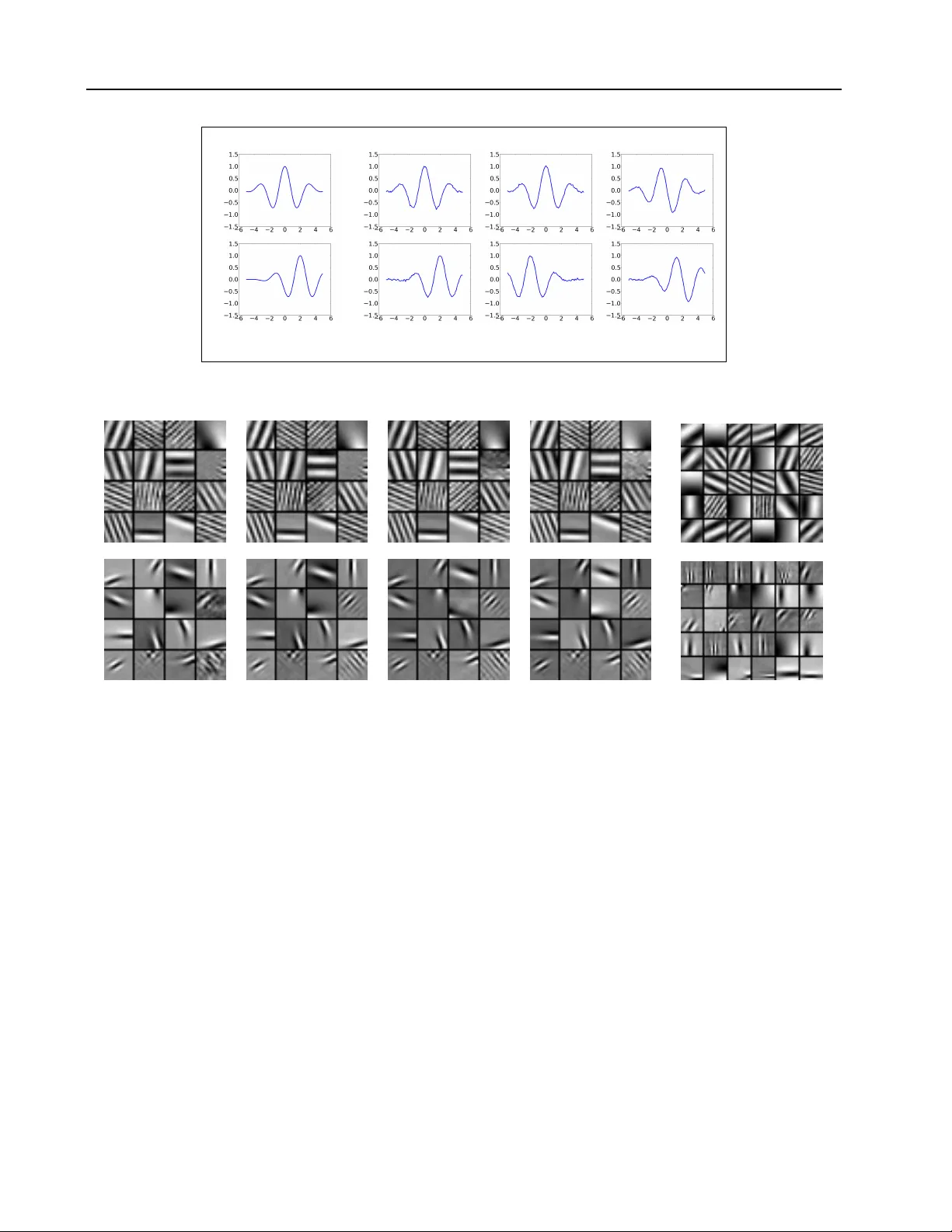
Learning to encode motion using spatio-temporal synchr ony Kishore K onda K O N DA @ I N F O R M AT I K . U N I - F R A N K F U RT . D E Goethe Univ ersity Frankfurt, Frankfurt Roland Memisevic RO L A N D . M E M I S E V I C @ U M O N T R E A L . C A Univ ersity of Montreal, Montreal V incent Michalski V M I C H A L S @ R Z . U N I - F R A N K F U RT . D E Goethe Univ ersity Frankfurt, Frankfurt Abstract W e consider the task of learning to extract motion from videos. T o this end, we show that the detec- tion of spatial transformations can be viewed as the detection of synchrony between the image se- quence and a sequence of features undergoing the motion we wish to detect. W e show that learn- ing about synchrony is possible using very fast, local learning rules, by introducing multiplica- tiv e “gating” interactions between hidden units across frames. This makes it possible to achie ve competitiv e performance in a wide variety of mo- tion estimation tasks, using a small fraction of the time required to learn features, and to outper- form hand-crafted spatio-temporal features by a large mar gin. W e also show ho w learning about synchrony can be viewed as performing greedy parameter estimation in the well-known motion energy model. 1. Introduction The classic motion energy model turns the frames of a video into a representation of motion by summing over squares of Gabor filter responses ( Adelson & Bergen , 1985 ; W at- son & Albert J. Ahumada , 1985 ). One of the motiv ations for this computation is the fact that sums over squared filter responses allo w us to detect “oriented” energies in spatio- temporal frequency bands. This, in turn, makes it possi- ble to encode motion independently of phase information, and thus to represent motion to some degree independent of what is mo ving. Related models hav e been proposed for binocular disparity estimation (e.g. Fleet et al. , 1996 ), which also in volves the estimation of the displacement of local features across multiple views. For many years, hand-crafted, Gabor-like filters ha ve been used (see, e.g., Derpanis , 2012 ), but in recent years, un- supervised deep learning techniques have become popu- lar which learn the features from videos (e.g. T aylor et al. , 2010 ; Le et al. , 2011 ; Ji et al. , 2013 ; Memisevic & Hinton , 2007 ), The interest in learning-based models of motion is fueled in part by the observ ation that for acti vity recogni- tion, hand-crafted features tend to not perform uniformly well across tasks ( W ang et al. , 2009 ), which suggests learn- ing the features instead of designing them by hand. Unlike images, videos hav e been somewhat resistant to fea- ture learning, in that many standard models do not w ork well. On images, for e xample, models lik e the autoencoder or even K-means clustering, are known to yield highly struc- tured, Gabor-like, filters, which perform well in recognition tasks ( Coates et al. , 2011 ). The same does not seem to be true for videos, where neither autoencoders nor K-means were sho wn to work well (see, for example, Section 4 ). There are two notable e xceptions: Feature learning models like ICA, where inference in volves a search over filters that are sparse and at the same time minimize squared recon- struction error , were shown to learn at least visually good filters (see, for e xample, ( Olshausen , 2003 ) and references in ( Hyv arinen et al. , 2009 ), Chapter 16). The other excep- tion are energy models, which compute sums over squared filter responses for inference, and which were shown to work well in activity recognition tasks (e.g. Le et al. , 2011 ). In this work, we propose a possible explanation for why some models work well on videos, and other models do not. W e sho w that a linear encoding permits the detection of transformations across time, because it supports the detec- tion of temporal “synchrony” between video and features. This makes it possible to interpret motion energy models as a way to combine two independent contributions to mo- tion encoding, namely the detection of synchrony , and the encoding of in variance. W e show how disentangling these two contributions provides a different perspectiv e onto the energy model and suggests new approaches to learning. In particular , we show that learning a linear encoding can be Learning to encode motion using spatio-temporal synchr ony viewed as learning in the presence of multiplicative “gat- ing” interactions (e.g. Mel , 1994 ). This allows us to learn competitiv e motion features on conv entional CPU-based hardware and in a small fraction of the time required by previous methods. 2. Motion from spatio-temporal synchr ony Consider the task of computing a representation of motion, giv en two frames ~ x 1 and ~ x 2 of a video. The classic energy model ( Adelson & Ber gen , 1985 ) solves this task by detect- ing subspace energy . This amounts to computing the sum of squared quadrature Fourier or Gabor coefficients across multiple frequencies and orientations (e.g. Hyvarinen et al. , 2009 ). The motiv ation behind the energy model is that Fourier amplitudes are independent of stimulus phase, so they yield a representation of motion that is to some degree independent of image content. As we shall show below , this view confounds two independent contributions of the energy model, which may be disentangled in practice. An alternative to computing the sum over squar es , which has originally been proposed for stereopsis, is the cross- correlation model ( Arndt et al. , 1995 ; Fleet et al. , 1996 ), which computes the sum over pr oducts of filter-responses across the two frames. It can be sho wn that the sum over products of filter responses in quadrature encodes angles in the in variant subspaces associated with the transformation. The representation of angles thereby also yields a phase- in variant representation of motion (e.g. Fleet et al. , 1996 ; Cadieu & Olshausen , 2011 ; Memisevic , 2012 ). Like the energy model, it also confounds inv ariance and represent- ing transformations as we shall show . It can be shown that cross-correlation models and energy models are closely related, and that there is a canonical op- eration that turns one into the other (e.g. Fleet et al. , 1996 ; Memisevic , 2012 ). W e shall revisit the close relationship between these models in Section 3.2 . 2.1. Motion estimation by synchrony detection W e shall no w discuss how synchrony detection allo ws us to compute motion, and how content-in variance can be achiev ed by pooling afterwards, if desired. T o this end, consider two filters ~ w 1 and ~ w 2 which shall encode the transformation between two images ~ x 1 and ~ x 2 . W e restrict our attention to transformations that can be represented as an orthogo- nal transformation in “pixel space”, in other words, as an orthogonal image warp. As these include all permutations, they include, in particular , most common spatial transfor- mations such as local translations and their combinations (see, e.g. Memisevic , 2012 , for a recent discussion). The assumption of orthogonality of transformations is made im- plicitly also by the motion energy model. T o detect an orthogonal transformation, P , between the two images, we propose to use filters for which ~ w 2 = P ~ w 1 (1) holds, and then to check whether the condition ~ w T 2 ~ x 2 = ~ w T 1 ~ x 1 (2) is true. W e shall call this the ”synchron y condition”. It amounts to choosing a filter pair , such that it is an example of the transformation we want to detect (Eq. 1 ), and to de- termine whether the two filters yield equal responses when applied in sequence to the two frames (Eq. 2 ). W e shall later relax the exact equality to an approximate equality . T o see why the synchron y condition counts as e vidence for the presence of the transformation, note first that ~ x 2 = P ~ x 1 implies ~ w T 2 ~ x 2 = ~ w T 2 P ~ x 1 . From this, we get: ~ x 2 = P ~ x 1 ( presence of P ) ⇒ ~ w T 2 ~ x 2  = ~ w T 2 P ~ x 1 = ( P T ~ w 2 ) T ~ x 1 =  ~ w T 1 ~ x 1 (3) The last equation follows from P T = P − 1 (orthogonality of P ). This shows that the presence of the transformation P implies synchron y (Eq. 2 ) for an y tw o filters which them- selves are related through P , that is ~ w 2 = P ~ w 1 . In order to detect the presence of P , we may thus look for the syn- chrony condition, using a set of filters transformed through P . This is an inductiv e (statistical) reasoning step, in that we can accumulate evidence for a transformation by look- ing for synchrony across multiple filters. The absence of the transformation implies that all filter pairs violate the synchrony condition. It is interesting to note that for Gabor filters, phase shifts and position shifts are locally the same (e.g. Fleet et al. , 1996 ). For global Fourier features, phase shifts and posi- tion shifts are exactly identical. Thus, synchrony (Eq. 1 ) between the inputs and a sequence of phase-shifted Fourier (or Gabor) features, for example, allows us to detect trans- formations which are local translations . W e shall discuss learning of filters from video data in Section 3 . The synchrony condition can be extended to a sequence of more than two frames as follows: Let ~ x i , ~ w i ( i = 1 , . . . , T ) denote the input frames and corresponding filters. T o detect a set of transformations P i , each of which relates two ad- jacent frames ( ~ x i , ~ x i +1 ) , set ~ w i +1 = P i ~ w i for all i . The condition for the presence of the sequence of transforma- tions now turns into ~ w T i ~ x i = ~ w T j ~ x j ∀ i, j = 1 , . . . , T and i 6 = j (4) Learning to encode motion using spatio-temporal synchr ony 2.2. The insufficiency of weighted summation T o check for the synchrony condition in practice, it is nec- essary to detect the equality of transformed filter responses across time (Eq. 2 ). Most current deep learning models are based on layers of weighted summation follo wed by a non- linearity . The detection of synchrony , unfortunately , cannot be performed in a layer of weighted summation plus non- linearity as we shall discuss now . The fact that the sum of filter responses, ~ w T 1 ~ x 1 + ~ w T 2 ~ x 2 , will attain its maximum for inputs that both match their fil- ters seems to suggest that thresholding it would allo w us to detect synchrony . This is not the case, howe ver , because thresholding works well only for inputs which are very sim- ilar to the feature vectors themselv es: Most inputs, in prac- tice, will be normalized superpositions of multiple feature vectors. Thus, to detect synchrony with a thresholded sum, we would need to use a threshold small enough to represent features, ~ w 1 , ~ w 2 , that e xplain only a fraction of the variabil- ity in ~ x 1 , ~ x 2 . If we assume, for example, that the two fea- tures ~ w 1 , ~ w 2 account for 50% of the variance in the inputs (an overly optimistic assumption), then we would hav e to reduce the threshold to be one half of the maximum attain- able response to be able to detect synchrony . Howe ver , at this lev el, there is no way to distinguish between two stim- uli which do satisfy the synchrony condition ( the motion in question is present ), and two stimuli where one image is a perfect match to its filter and the other has zero ov erlap with its filter ( the motion in question is not present ). The situation can only become worse for feature vectors that account for less than 50% of the variability . 2.3. Synchrony detection using multiplicati ve interactions If one is willing to abandon weighted sums as the only al- low able type of module for constructing deep networks, then a simple way to detect synchrony is by allowing for multiplicativ e (“gating”) interactions between filter responses: The product p = ~ w T 2 ~ x 2 · ~ w T 1 ~ x 1 (5) will be large only if ~ w T 2 ~ x 2 and ~ w T 1 ~ x 1 both take on large (or both v ery ne gativ e) v alues. Any suf ficiently small response of either ~ w T 2 ~ x 2 or ~ w T 1 ~ x 1 will shut of f the response of p , regardless of the filter response on the other image. That way , e ven a lo w threshold on p will not sacrifice our ability to differentiate between the presence of some feature in one of the images vs. the partial presence of the transformed feature in both of the images (synchrony). A related, less formal, argument for product interactions is that synchrony detection amounts to an operation akin to a logical “ AND”. This is at odds with the observation that weighted sums “accumulate” information and resemble a logical “OR” rather than an “ AND” (e.g. Zetzsche & Nud- ing , 2005 ). 2.4. A locally learned gating module It is important to note that multiplicativ e interactions will allow us to check for the synchrony condition using entirely local operations: Figure 1 illustrates how we may define a “neuron” that can detect synchrony by allowing for gating interactions within its “dendritic tree”. A model consist- ing of multiple of these synchron y detector units will be a single-layer model, as there is no cross-talk required be- tween the units. As we shall sho w , this fact allows us to use very fast local update rules for learning synchrony from data. This is in stark contrast to the learning of energy models and bi-linear models (e.g. Grimes & Rao , 2005 ; Hyv ¨ arinen & Hoyer , 2000 ; Memisevic & Hinton , 2007 ; Bethge et al. , 2007 ; T aylor et al. , 2010 ), which rely on non-local com- putations, such as back-prop, for learning (see also, Sec- tion 2.5 ). Although multiplicativ e interactions have been a common ingredient in most of these models their motiv a- tion has been that they allow for the computation of sub- space ener gies or subspace angles rather than synchrony (eg. Memise vic , 2012 ). The usefulness of intra-dendritic gating has been discussed at lengths in the neuroscience literature, for example, in the work by Mel and colleagues (e.g. Archie & Mel , 2000 ; Mel , 1994 ). But besides multi-layer bilinear models dis- cussed abov e, it has not recei ved much attention in ma- chine learning. Dendritic gating is reminiscent also of “Pi- Sigma” neurons ( Shin & Ghosh , 1991 ), which have been applied to some supervised prediction tasks in the past. Figure 1. Gating within a “dendritic tree. ” 2.5. Pooling and ener gy models Figure 2 shows an illustration of a product response using a 1-D example. The figure sho ws ho w the product of trans- formed filters and inputs yields a large response whenev er (i) the input is well-represented by the filter and (ii) the Learning to encode motion using spatio-temporal synchr ony input ev olves over time in a similar way as the filter (sec- ond column in the figure). The figure also illustrates how failing to satisfy either (i) or (ii) will yield a small prod- uct response (two rightmost columns). The need to satisfy condition (i) makes the product response dependent on the input. This dependency can be alle viated by pooling over multiple products, inv olving multiple different filters, such that the top-le vel pooling unit fires, if any subset of the synchrony detectors fires. The classic energy model, for example, pools over filter pairs in quadrature to eliminate the dependence on phase ( Adelson & Bergen , 1985 ; Fleet et al. , 1996 ). In practice, howe ver , it is not just phase but also frequency , position and orientation (or entirely differ- ent properties for non-Fourier features), which will deter- mine whether an image is aligned with a filter or not. W e in vestigate pooling with a separately trained pooling layer in Section 3 . 3. Learning synchr ony from data W e now discuss how to learn filters which allow us to de- tect the synchrony condition. There are in principle many ways to achieve this in practice, and we introduce a tempo- ral v ariant of the K-means algorithm to learn synchron y . In Appendix A we present another model based on the con- tractiv e autoencoder ( Rifai et al. , 2011 ), which we call syn- chrony autoencoder (SAE). In the following, we let ~ x, ~ y ∈ R N denote images, and we let W x , W y ∈ R Q × N denote matrices whose ro ws contain Q feature vectors, which we will denote by ~ W x q , ~ W y q ∈ R N . 3.1. Synchrony K-means Online K-means clustering has recently been shown to yield efficient, and highly competitive image features for objec- tiv e recognition ( Coates et al. , 2011 ). W e first note that, given a set of Q cluster centers ~ W x q , per - forming online gradient-descent on the standard (not syn- chrony) K-means clustering objectiv e is equiv alent to up- dating the cluster centers using the local competiti ve learn- ing rule ( Rumelhart & Zipser , 1986 ) ∆ ~ W x s = η ( ~ x − ~ W x s ) (6) where η is a step-size and s is the “winner-takes-all” as- signment s = arg min q k ~ x − ~ W x q k 2 (7) When cluster-centers (“features”) are contrast-normalized, the assignment function is equiv alent to s = arg max q [( ~ W x q ) T ~ x ] (8) W ith the online K-means rule in mind, we no w define a synchrony K-means (SK-means) model as follows. W e define the synchrony condition by first introducing multi- plicativ e interactions in the assignment function: s = arg max q [(( ~ W x q ) T ~ x )(( ~ W y q ) T ~ y )] (9) Note that computing the multiplication is equiv alent to re- placing the K-means winner-takes-all units by gating units (cf., Figure 1 ). This allows us to redefine the K-means objectiv e function to be the reconstruction error between one input and the assigned prototype vector , which is gated (multiplied elementwise) with the projection of the other input: L x = ( ~ x − ~ W x s (( ~ W y s ) T ~ y )) 2 (10) The gradient of the reconstruction error is ∂ L x ∂ ~ W x s = − 4( ~ x ( ~ W y s ) T ~ y − ~ W x s (( ~ W y s ) T ~ y ) 2 ) (11) This allows us to define the synchr ony K-means learning rule : ∆ ~ W x s = η ( ~ x ( ~ W y s ) T ~ y − ~ W x s (( ~ W y s ) T ~ y ) 2 ) (12) Similar to the online-kmeans rule ( Rumelhart & Zipser , 1986 ), we obtain a Hebbian term ~ x ( ~ W y s ) T ~ y , and an “active forgetting” term ( ~ W x s (( ~ W y s ) T ~ y ) 2 ) which enforces compe- tition among the hiddens. The Hebbian term, in contrast to standard K-means, is “gated”, in that it inv olves both the “pre-synaptic” input ~ x , and the projected pre-synaptic input ( ~ W y s ) T ~ y coming from the other input. Similarly the update rule for ~ W y s is giv en by ∆ ~ W y s = η ( ~ y ( ~ W x s ) T ~ x − ~ W y s (( ~ W x s ) T ~ x ) 2 ) (13) 3.2. Synchrony detection using e ven-symmetric non-linearities As defined in Section 2.1 , ~ x i , ~ w i ( i = 1 , . . . , T ) denote the input frames and corresponding filters. An e ven-symmetric nonlinearity with global minimum at zero, such as the square function, applied to P i ~ w T i ~ x i , will be a detector of the syn- chrony condition, too. The reason is the binomial identity , which states that the square of the sum of terms contains the pair-wise products between all individual terms plus the squares of the indi vidual terms. The latter do not change the preferred stimulus of the unit ( Fleet et al. , 1996 ; Memi- sevic , 2012 ). The value of ( P i ~ w T i ~ x i ) 2 is high only when the indi vidual terms are equal to each other and of high value, i.e, ~ w T i ~ x i = ~ w T j ~ x j which is the synchron y condition in case of sequences (Equation 4 ). Squaring non-linearities applied to the sum of phase-shifted Gabor filter responses hav e been the cornerstone of the ener gy model ( Adelson & Bergen , 1985 ; W atson & Albert J. Ahumada , 1985 ; Hyvari- nen et al. , 2009 ). Learning to encode motion using spatio-temporal synchr ony case-1 case-2 case-3 ~ w 1 ~ x 1 ~ w 2 ~ x 2 p = 1231 . 02 p = 37 . 52 p = − 0 . 002 Figure 2. Demonstration of product responses p with two filters ~ w 1 , ~ w 2 encoding a translation P . case-1: ~ x 2 = P ~ x 1 ; case-2: ~ x 2 6 = P ~ x 1 ; case-3: ~ x 2 = P ~ x 1 but ~ x 1 and ~ w 1 are out of phase by π / 2 . Figure 3. Row 1: Filters learned on synthetic translations of natural image patches. Row 2: Filters learned on natural videos. Columns 1-4: Frames 1-4 of the learned filters. Column 5: Filter groupings learned by a separate layer of K-means (only first frame filters shown). Each row in column 5 sho ws the six filters contributing the most to that cluster center . Even-symmetric non-linearities implicitly compute pair-wise products and they may be implemented using multiplica- tiv e interactions, too: Consider the unit in Figure 1 , using “tied” inputs ~ x 1 = ~ x 2 , and assume that they contain a video sequence rather than a single image. If we also use tied weights ~ w 1 = ~ w 2 , then the output, p , of this unit will be equal to the square of ~ w T 1 ~ x 1 . In practice, the model can learn to tie weights, if required. T o enable the model from Section 3.1 to encode motion across multiple frames, we may thus proceed as follows: Let ~ X ∈ R N be the concatenation of T frames ~ x t ∈ R M , t = 1 , . . . , T , and let W ∈ R Q × N denote the matrix containing the Q feature vectors ~ W q ∈ R N stacked row-wise. Each feature is composed of frame features ~ w q t ∈ R M where each ~ w q t spans one frame ~ x t from the input video. The SK-means can be adapted to sequences by replacing frames ~ x, ~ y with a sequence ~ X and tying the weights W x , W y to W . The update rule for the SK-means model now be- comes ∆ ~ W s = η ( ~ X ( ~ W T s ~ X ) − ~ W s ( ~ W T s ~ X ) 2 ) (14) where the assignment function s is s ( ~ X ) = arg max q [( ~ W T q ~ X ) 2 ] (15) Note that computing the square of P t ~ w T q t ~ x t abov e also accounts for synchrony as e xplained earlier . For inference in case of the SK-means model, we use a sigmoid activ ation function on the squared features in our experiments instead of winner -takes-all (cf., Eq. 15 ). As in the case of object classification ( Coates et al. , 2011 ), relax- ing the harsh sparsity induced by K-means tends to yield codes better suited for recognition tasks. Learning to encode motion using spatio-temporal synchr ony Example filters learned with the contracti ve SAE on se- quences are shown in Figure 3 . In the first row of the fig- ure, columns 1 to 4 sho w filters learned on 50 , 000 syn- thetic movies generated by translating image patches from the natural image dataset in ( Martin et al. , 2001 ). Columns 1 to 4 of the second ro w sho w filters learned on blocks sam- pled from videos of a broadcast TV database in ( Hateren & Schaaf , 1998 ). W e obtained similar filters using the SK- means model. 3.3. Learning a separate pooling layer T o study the dependencies of features, we performed K- means clustering, using 500 centroids, on the hiddens ex- tracted from the training sequences. Column 5 of Figure 3 shows, for the most acti ve clusters across the training data, the six features which contribute the most to each of the cluster centers. It sho ws that the “pooling units” (clus- ter centers) group together features with similar orientation and position, and with arbitrary frequency and phase. This is to be expected, as translation in any direction will af- fect all frequencies and phase angles, and only “nearby” orientations and positions. Note in particular , that pooling across phase angles alone, as done by the classic energy model, would not be sufficient, and it is, in fact, not the solution found by pooling. 4. A pplication to activity recognition Activity recognition is a common task for ev aluating mod- els of motion understanding. T o allow for a fair compar- ison, we use the same pipeline as described in ( Le et al. , 2011 ; W ang et al. , 2009 ), using the features learned by our models. W e train our models on pca-whitened input patches of size 10 × 16 × 16 . The number of training sam- ples is 200 , 000 . The number of product units are fixed at 300 . For inference sub blocks of the same size as the patch size are cropped from “super blocks” of size 14 × 20 × 20 ( Le et al. , 2011 ). The sub blocks are cropped with a stride of 4 on each axis giving 8 sub blocks per su- per block. The feature responses of sub blocks are con- catenated and dimensionally reduced using PCA to form the local feature. Using a separate layer of K-means, a vocab ulary of 3000 spatio-temporal words is learned with 500 , 000 samples for training. In all our experiments the super blocks are cropped densely from the video with a 50% overlap. Finally , a χ 2 -kernel SVM on the histogram of spatio-temporal words is used for classification. 4.1. Datasets W e e v aluated our models on se veral popular activity recog- nition benchmark datasets: KTH ( Schuldt et al. , 2004 ): Six actions performed by 25 T able 1. A verage accurac y on KTH. A L G O R I T H M P E R F O R M A N C E ( % ) SAE 9 3 . 5 SK-means 9 3 . 6 G R B M ( T AY L OR E T A L . , 2 0 1 0 ) 9 0 . 0 I S A M O D E L ( L E E T A L . , 2 0 1 1 ) 9 3 . 9 T able 2. A verage accurac y on UCF sports. A L G O R I T H M P E R F O R M A N C E ( % ) SAE 8 6 . 0 SK-means 8 4 . 7 I S A M O D E L ( L E E T A L . , 2 0 1 1 ) 8 6 . 5 subjects. Samples divided into train and test data accord- ing to the authors original split. The multi-class SVM is directly used for classification. UCF sports( Rodriguez et al. , 2008 ): T en action classes. The total number of videos in the dataset is 150. T o in- crease the data we add horizontally flipped version of each video to the dataset. Like in ( Rodriguez et al. , 2008 ) we train a multi-class SVM for classification, and we use leave- one-out for e valuation. That is, each original video is tested with all other videos as training set except the flipped ver- sion of the one being tested and itself. Hollywood2 ( Marszałek et al. , 2009 ): T welve activity classes. It consists of 884 test samples and 823 train samples with some of the video samples belonging to multiple classes. Hence, a binary SVM is used to compute the average pre- cision (AP) of each class and the mean AP ov er all classes is reported ( Marszałek et al. , 2009 ). YUPENN dynamic scenes ( Derpanis , 2012 ): Fourteen scene categories with 30 videos for each category . W e only use the gray-scale version of the videos in our experiments. Leav e-one-out cross-validation is used for performance ev al- uation ( Derpanis , 2012 ). T able 3. Mean AP on Hollywood2. A L G O R I T H M P E R F O R M A N C E ( % ) SAE 5 1 . 8 SK-means 5 0 . 5 G R B M ( T AY L OR E T A L . , 2 0 1 0 ) 4 6 . 6 I S A M O D E L ( L E E T A L . , 2 0 1 1 ) 5 3 . 3 C O V A E ( M E M I S E V I C , 2 0 1 1 ) 4 3 . 3 Learning to encode motion using spatio-temporal synchr ony T able 4. A verage accurac y on YUPENN. A L G O R I T H M P E R F O R M A N C E ( % ) SAE ( K - N N ) 8 0. 7 SAE ( χ 2 S V M ) 9 6 . 0 SK-means ( χ 2 S V M ) 9 5 . 2 S O E ( D E R P A N I S , 2 0 1 2 ) 7 9 . 0 T able 5. Performance on column dataset using SAE trained on row dataset. D AT A S E T K T H U C F H O L L Y W O O D 2 K T H 9 3 . 5 8 5 . 3 4 4 . 7 U C F 9 2 . 9 8 6 . 0 4 8 . 9 H O L LY W O O D 2 92 . 7 8 5 . 3 5 1 . 8 4.2. Results The results are shown in T ables 1 , 2 , 3 and 4 . They show that the SAE and SK-means are competiti ve with the state- of-the-art, although learning is simpler than for most e xist- ing methods. T o ev aluate the importance of element-wise products of hidden units, we also e valuated K-means as well as a standard autoencoder with contraction as regular - ization on the Hollywood2 dataset. The models achiev ed an average precision of 42 . 1 and 42 . 7 respectiv ely , which is much lower than the performance from SAE and SK- means. W e also tested the cov ariance auto-encoder ( Memi- sevic , 2011 ), which learns an additional mapping layer that pools over squared simple cell responses. T able 3 shows that the performance of this model is also considerably lower than our single-layer models, sho wing that learning the pool- ing layer along with features did not help. 4.3. Unsupervised learning and dataset bias T o show that our models learn features that can generalize across datasets (“self-taught learning” ( Le et al. , 2011 )), we trained SAE on random samples from one of the datasets and used it for feature extraction to report performance on the others. The performances using the same metrics as before are shown in table 5 . It can be seen that the perfor- mance gets reduced by only a fairly small fraction as com- pared to training on samples from the respective dataset. Only in the case where training on the KTH dataset, per- formance on Hollywood2 is considerably lo wer . This is probably due to the less div erse activities in KTH as com- pared to those in Hollywood2. T able 6. Training time. A L G O R I T H M T I M E SK-means ( G P U ) 2 M I N U T E S SK-means ( C P U ) 3 M I N U T E S SAE ( G P U ) 1 − 2 H O U R S I S A ( L E E T A L . , 2 0 1 1 ) 1 − 2 H O U R S G R B M ( T A Y L O R E T A L . , 2 0 1 0 ) 2 − 3 D AYS 4.4. Computational efficiency T raining times for learning the motion features are shown in T able 6 . They show that SK-means (trained on CPU) is orders of magnitude faster than all other models. For the GPU implementations, we used the theano library ( Bergstra et al. , 2010 ). W e also calculated inference times using a similar metric as ( Le et al. , 2011 ) and computed the time required to extract descriptors for 30 videos from the Hol- lywood2 dataset with resolution 360 × 288 pix els (with “sigmoid-of-square” hiddens they are identical for SK-means or SAE). A verage inference times (in seconds/frame) were 0 . 058 on CPU and 0 . 051 on GPU, making the models fea- sible in practical, and possibly real-time, applications. All experiments were performed on a system with a 3 . 20 GHz CPU, 24 GB RAM and a GTX 680 GPU. 5. Conclusions Our work sho ws that learning about motion from videos can be simplified and significantly sped up by disentangling learning about the spatio-temporal evolution of the signal from learning about in variances in the inputs. This allows us to achieve competitiv e performance in activity recogni- tion tasks at a fraction of the computational cost for learn- ing motion features required by existing methods, such as the motion energy model ( Le et al. , 2011 ). W e also sho wed how learning about motion is possible using entirely local learning rules. Computing products by using “dendritic gating” within in- dividual, but competing, units may be viewed as an efficient compromise between bi-linear models, that are expensiv e because they encode interactions between all pairs of pix- els ( Grimes & Rao , 2005 ; Memisevic & Hinton , 2007 ; Ol- shausen et al. , 2007 ), and “factored” models (e.g. Cadieu & Olshausen , 2011 ; T aylor et al. , 2010 ; Memise vic , 2012 ), which are multi-layer models that rely on more compli- cated training schemes such as back-prop and which do not work as well for recognition. Acknowledgments: This work was supported in part by the German Federal Ministry of Education and Research (BMBF) in project 01GQ0841 (BFNT Frankfurt), by an Learning to encode motion using spatio-temporal synchr ony NSERC Discovery grant and by a Google faculty research award. A. Synchrony autoencoder Here we present an additional approach to encoding motion across tw o frames, based on the contracti ve autoencoder ( Rifai et al. , 2011 ). Like the synchrony K-means algorithm, it can be extended to sequences with more than two frames, using an analogous construction (cf., Section 3.2 ). Gi ven two images, we first compute the linear filter responses ~ f x = W x ~ x and ~ f y = W y ~ y . Giv en the deri vations in Sec- tion 2 , an encoding of the motion, ~ h = ~ h ( ~ x, ~ y ) , inherent in the image sequence may then be defined as ~ h = σ ( ~ f x  ~ f y ) (16) where  is element-wise multiplication and σ is the sig- moid nonlinearity (1 + exp( − x )) − 1 . This definition makes sense only , if features vectors are related by the transforma- tion we wish to detect. W e shall now discuss how we can define a reconstruction criterion that enforces this criterion. The standard way to train an autoencoder on images is to add a decoder and to minimize reconstruction error . In our case, because of the presence of multiplicativ e interactions in the encoder , the encoding loses information about the sign of the input. Howe ver , note that we may interpret the multiplicativ e interactions as gating as discussed in the pre- vious section. This suggests defining the reconstruction er - ror on one input, giv en the other . In the decoder we thus perform an element-wise multiplication of the hiddens and factors of one of the input to reconstruct the other . One may also view this as re-introducing the sign information at reconstruction time. Assuming an autoencoder with tied weights, the reconstructed inputs can then be defined as ˆ x = ( W x ) T ( ~ h  ~ f y ) (17) ˆ y = ( W y ) T ( ~ h  ~ f x ) (18) W e define the reconstruction error as the average squared difference between the two inputs and their respectiv e re- constructions: L (( ~ x, ~ y ) , ( ˆ ~ x, ˆ ~ y )) = k ( ~ x − ˆ ~ x ) k 2 + k ( ~ y − ˆ ~ y ) k 2 (19) Learning amounts to minimizing the reconstruction error wrt. the filters ( W x ) and ( W y ) . In contrast to bi-linear models, which may be trained using similar criteria (e.g. Memisevic , 2011 ; T aylor et al. , 2010 ), the representation of motion in Eq. 16 will be dependent on the image content, such as F ourier phase for translational motion. But this de- pendence can be removed using a separately trained pool- ing layer as we shall show . The absence of pooling during feature learning allows for much more efficient learning as we show in Section 4 . Note that, in practice, one may add bias terms to the definition of hiddens and reconstructions. A.1. Contractive r egularization It is well-known that regularization is important to extract useful features and to learn sparse representations. Here, we use contraction as regularization ( Rifai et al. , 2011 ). This amounts to adding the Frobenius norm of the Jaco- bian of the extracted features, i.e., the sum of squares of all partial deriv ati ves of ~ h with respect to ~ x, ~ y k J e ( ~ x, ~ y ) k 2 E = X ij  ∂ h j ( ~ x, ~ y ) ∂ x i  2 + X ij  ∂ h j ( ~ x, ~ y ) ∂ y i  2 (20) which for the sigmoid-of-square non-linearity becomes k J e ( ~ x, ~ y ) k 2 E = P j ( h j (1 − h j )) 2 ( f x j ) 2 P i ( W y ij ) 2 + P j ( h j (1 − h j )) 2 ( f y j ) 2 P i ( W x ij ) 2 (21) For training, we add the regularization term to the recon- struction cost, using a hyperparameter λ . Contracti ve reg- ularization is not possible in (multi-layer) bi-linear mod- els, due to the computational complexity of computing the contraction gradient for multiple layers (e.g. Memise vic , 2011 ). Being a single layer model, the synchrony autoen- coder (SAE) makes the application of contractiv e regular - ization feasible. The contraction parameter λ are set by cross-validation. The SAE can be adapted to sequences by replacing frames ~ x, ~ y with a sequence ~ X and tying the weights W x , W y to W . The representation of motion from Equation 16 can now be redefined as, H q = σ ( F 2 q ) = σ  (( ~ W q ) T ~ X ) 2  = σ  ( X t ~ w T q t ~ x t ) 2  (22) Note that computing the square of P t ~ w T q t ~ x t abov e also accounts for synchrony as e xplained earlier . The recon- struction error and regularization term for this model can be deri ved by just replacing appropriate terms in Equations 19 and 21 , respectiv ely . References Adelson, Edward H. and Ber gen, James R. Spatiotemporal energy models for the perception of motion. J. OPT . SOC. AM. A , 2(2):284–299, 1985. Archie, Ke vin A. and Mel, Bartlett W . A model for in- tradendritic computation of binocular disparity . Natur e Neur oscience , 3(1):54–63, January 2000. Arndt, P .A., Mallot, H.A., and B ¨ ulthoff, H.H. Human stere- ovision without localized image features. Biological cy- bernetics , 72(4):279–293, 1995. Bergstra, James, Breuleux, Olivier , Bastien, Fr ´ ed ´ eric, Lamblin, Pascal, Pascanu, Razv an, Desjardins, Guil- laume, Turian, Joseph, W arde-Farley , Da vid, and Ben- gio, Y oshua. Theano: a CPU and GPU math expression compiler . In SciPy , 2010. Learning to encode motion using spatio-temporal synchr ony Bethge, M, Gerwinn, S, and Macke, JH. Unsupervised learning of a steerable basis for in variant image repre- sentations. In Human V ision and Electronic Imaging XII . SPIE, 2007. Cadieu, Charles F . and Olshausen, Bruno A. Learning Intermediate-Lev el Representations of F orm and Motion from Natural Movies. Neural Computation , 24(4):827– 866, December 2011. Coates, Adam, Lee, Honglak, and Ng, A. Y . An analysis of single-layer networks in unsupervised feature learning. In Artificial Intelligence and Statistics , 2011. Derpanis, Konstantinos G. Dynamic scene understand- ing: The role of orientation features in space and time in scene classification. In CVPR , 2012. Fleet, D., W agner , H., and Heeger , D. Neural encoding of binocular disparity: Energy models, position shifts and phase shifts. V ision Resear ch , 36(12):1839–1857, June 1996. Grimes, David and Rao, Rajesh. Bilinear sparse coding for inv ariant vision. Neur al Computation , 17(1):47–73, 2005. Hateren, J. H. v an and Schaaf, A. van der . Independent component filters of natural images compared with sim- ple cells in primary visual cortex. Pr oceedings: Biolog- ical Sciences , 265(1394):359–366, Mar 1998. Hyv ¨ arinen, Aapo and Hoyer , Patrik. Emergence of phase- and shift-inv ariant features by decomposition of natural images into independent feature subspaces. Neural Com- put. , 12:1705–1720, July 2000. Hyvarinen, Aapo, Hurri, Jarmo, and Hoyer , P atrick O. Nat- ural Image Statistics: A Pr obabilistic Appr oach to Early Computational V ision . Springer Publishing Company , Incorporated, 2009. Ji, Shuiwang, Xu, W ei, Y ang, Ming, and Y u, Kai. 3D con- volutional neural networks for human action recognition. IEEE T ransactions on P attern Analysis and Machine In- telligence , 35(1):221–231, 2013. Le, Q.V ., Zou, W .Y ., Y eung, S.Y ., and Ng, A.Y . Learn- ing hierarchical in variant spatio-temporal features for ac- tion recognition with independent subspace analysis. In CVPR , 2011. Marszałek, Marcin, Laptev , Ivan, and Schmid, Cordelia. Actions in context. In IEEE Confer ence on Computer V ision & P attern Recognition , 2009. Martin, D., Fo wlkes, C., T al, D., and Malik, J. A database of human segmented natural images and its application to ev aluating segmentation algorithms and measuring ecological statistics. In ICCV , 2001. Mel, Bartlett W . Information processing in dendritic trees. Neural Computation , 6(6):1031–1085, 1994. Memisevic, Roland. Gradient-based learning of higher - order image features. In ICCV , 2011. Memisevic, Roland. On multi-vie w feature learning. In ICML , 2012. Memisevic, Roland and Hinton, Geof frey . Unsupervised learning of image transformations. In CVPR , 2007. Olshausen, B.A. Learning sparse, overcomplete represen- tations of time-varying natural images. In Image Pr o- cessing, 2003. ICIP 2003. Pr oceedings. 2003 Interna- tional Confer ence on , volume 1, pp. I–41–4 vol.1, Sept 2003. Olshausen, Bruno, Cadieu, Charles, Culpepper , Jack, and W arland, David. Bilinear models of natural images. In SPIE Pr oceedings: Human V ision Electr onic Imaging XII , San Jose, 2007. Rifai, Salah, V incent, Pascal, Muller , Xavier , Glo- rot, Xavier , and Bengio, Y oshua. Contractiv e Auto- Encoders: Explicit In variance During Feature Extrac- tion. In ICML , 2011. Rodriguez, Mikel D., Ahmed, Jav ed, and Shah, Mubarak. Action mach: a spatio-temporal maximum average cor- relation height filter for action recognition. In CVPR , 2008. Rumelhart, D. E. and Zipser , D. Parallel distributed pro- cessing: explorations in the microstructure of cognition, vol. 1. chapter Feature discovery by competitive learn- ing, pp. 151–193. MIT Press, 1986. Schuldt, C., Lapte v , I., and Caputo, B. Recognizing human actions: a local svm approach. In P attern Recognition, 2004. ICPR 2004. Pr oceedings of the 17th International Confer ence on , 2004. Shin, Y oan and Ghosh, Joydeep. The pi-sigma network: An efficient higher-order neural netw ork for pattern clas- sification and function approximation. In International Joint Confer ence on Neural Networks , 1991. T aylor , Graham W ., Fergus, Rob, LeCun, Y ann, and Bregler , Christoph. Conv olutional learning of spatio- temporal features. In Proceedings of the 11th Eur opean confer ence on Computer vision: P art VI , ECCV’10, 2010. W ang, Heng, Ullah, Muhammad Muneeb, Kl ¨ aser , Alexan- der , Laptev , Ivan, and Schmid, Cordelia. Evaluation of local spatio-temporal features for action recognition. In University of Central Florida, U .S.A , 2009. W atson, Andrew B. and Albert J. Ahumada, Jr . Model of human visual-motion sensing. J. Opt. Soc. Am. A , 2(2): 322–341, Feb 1985. Zetzsche, Christoph and Nuding, Ulrich. Nonlinear and higher-order approaches to the encoding of natural scenes. Network (Bristol, England) , 16(2-3):191–221, 2005.