Computing all maps into a sphere

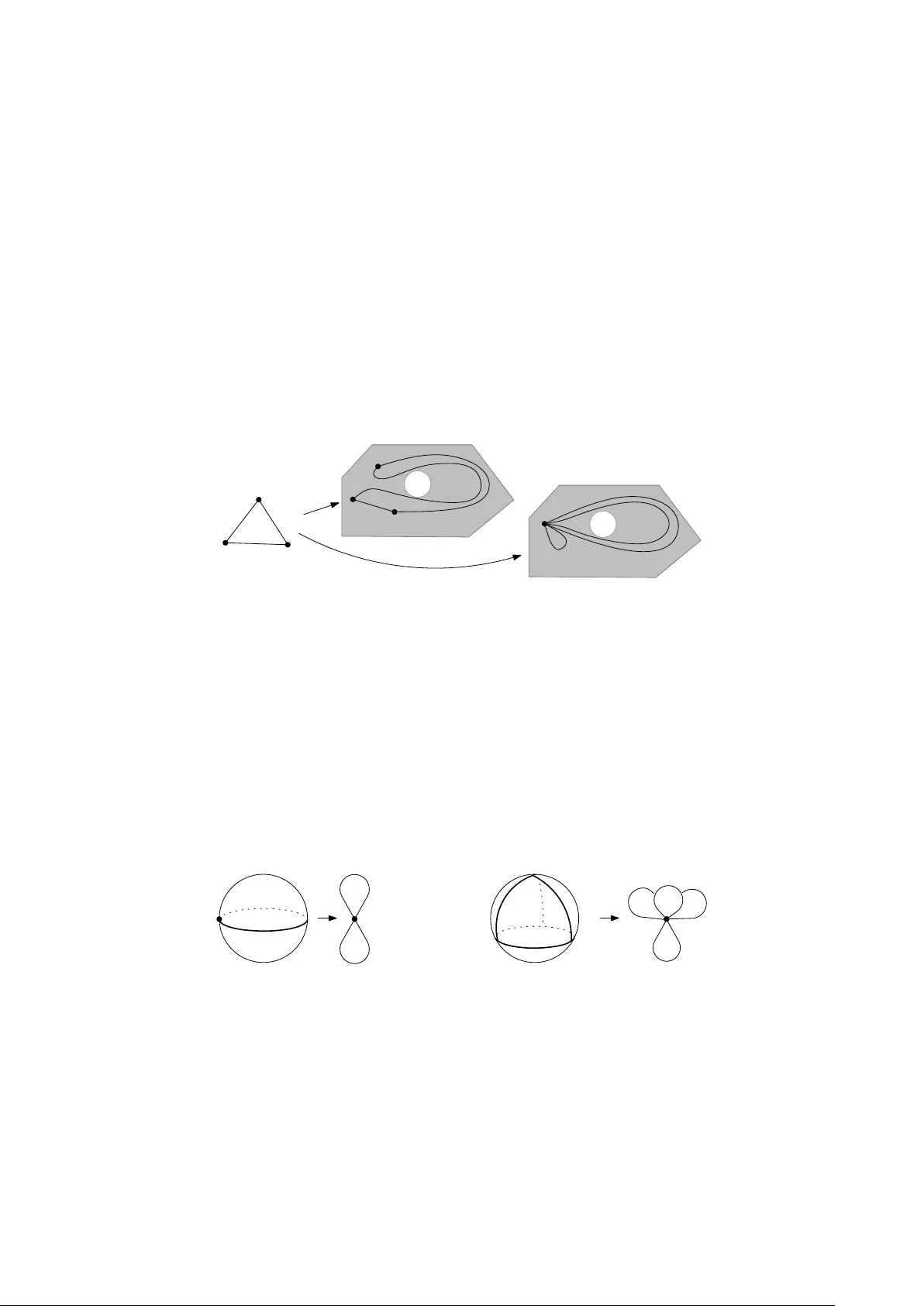
Computing all maps in to a sphere ∗ Martin ˇ Cadek a Marek Kr ˇ c´ al b , c Ji ˇ r ´ ı Matou ˇ sek b , d F rancis Sergeraert e Luk´ a ˇ s V ok ˇ r ´ ınek a Uli W agner c Ma y 28, 2018 Abstract Giv en top ological spaces X , Y , a fundamental problem of algebraic top ology is under- standing the structure of all con tin uous maps X → Y . W e consider a computational version, where X, Y are giv en as ﬁnite simplicial complexes, and the goal is to compute [ X , Y ], i.e., all homotopy classes of such maps. W e solve this problem in the stable r ange , where for some d ≥ 2, we ha ve dim X ≤ 2 d − 2 and Y is ( d − 1) -c onne cte d ; in particular, Y can b e the d -dimensional sphere S d . The al- gorithm com bines classical to ols and ideas from homotopy theory ( obstruction the ory , Post- nikov systems , and simplicial sets ) with algorithmic to ols from eﬀective algebraic top ology ( lo c al ly eﬀe ctive simplicial sets and obje cts with eﬀe ctive homolo gy ). In contrast, [ X, Y ] is known to b e uncomputable for general X , Y , since for X = S 1 it includes a well known undecidable problem: testing triviality of the fundamental group of Y . In follow-up pap ers, the algorithm is sho wn to run in p olynomial time for d ﬁxed, and extended to other problems, such as the extension pr oblem , where we are given a subspace A ⊂ X and a map A → Y and ask whether it extends to a map X → Y , or computing the Z 2 -index —ev erything in the stable range. Outside the stable range, the extension problem is undecidable. 1 In tro duction Among results concerning computations in top ology , probably the most famous ones are neg- ativ e. F or example, there is no algorithm to decide whether the fundamen tal group π 1 ( Y ) of a given space Y is trivial, i.e., whether every lo op in Y can b e contin uously contracted to a p oin t. 1 Here w e obtain a p ositiv e result for a closely related and fairly general problem, homotop y classiﬁcation of maps; 2 namely , we describ e an algorithm that works in the so-called stable r ange . * The research b y M. ˇ C. and L. V. was supported by a Czech Ministry of Education grant (MSM 0021622409). The research by M. K. was supp orted by pro ject GAUK 49209. The research by J. M. and M. K. was also supp orted by pro ject 1M0545 by the Ministry of Education of the Czec h Republic and b y Center of Excellence – Inst. for Theor. Comput. Sci., Prague (pro ject P202/12/G061 of GA ˇ CR). The research b y J. M. was also supp orted by the ERC Adv anced Gran t No. 267165. The research b y U. W. was supported by the Swiss National Science F oundation (SNF Pro jects 200021-125309, 200020-138230, and PP00P2-138948). a Departmen t of Mathematics and Statistics, Masaryk Universit y , Kotl´ a ˇ rsk´ a 2, 611 37 Brno, Czech Republic b Departmen t of Applied Mathematics, Charles Universit y , Malostransk´ e n´ am. 25, 118 00 Praha 1, Czech Republic c IST Austria, Am Campus 1, 3400 Klosterneuburg, Austria, d Departmen t of Computer Science, ETH Z ¨ uric h, 8092 Z¨ uric h, Switzerland e Institut F ourier, BP 74, 38402 St Martin, d’H` eres Cedex, F rance 1 This follows by a standard reduction, see, e.g., [ 54 ], from a result of Adjan and Rabin on unsolv ability of the trivialit y problem of a group given in terms of generators and relation; see, e.g., [ 51 ]. 2 The deﬁnition of homotopy and other basic top ological notions will b e recalled later. 1 Computational top ology . This pap er falls into the broader area of c omputational top olo gy , whic h has b een a rapidly developing discipline in recen t years—see, for instance, the textb o oks [ 12 , 58 , 33 ]. Our fo cus is somewhat diﬀeren t from the main current trends in the ﬁeld, where, on the one hand, computational questions are intensiv ely studied in dimensions 2 and 3 (e.g., concerning gr aphs on surfac es , knots or 3 -manifolds 3 ), and, on the other hand, for arbitrary dimensions mainly homolo gy computations are in vestigated. Homology has been considered an inherently computational tool s ince its inception and there are many softw are pack ages that con tain practical implemen tations, e.g., polymake [ 19 ]. Thus, algorithmic solv ability of homological questions is usually obvious, and the challenge may b e, e.g., designing very fast algorithms to deal with large inputs. Moreov er, lot of research has b een dev oted to developing extensions such as p ersistent homolo gy [ 11 ], motiv ated by applications lik e data analysis [ 9 ]. In contrast, homotopy-the or etic pr oblems , as those studied here, are generally considered m uch less tractable than homological ones and the ﬁrst question to tac kle is usually the existence of an y algorithm at all (indeed, many of them are algorithmically unsolv able, as the example of triviality of the fundamental group illustrates). Suc h problems lie at the core of algebraic top ology and hav e b een thoroughly studied from a top ological p ersp ective since the 1940s. A signiﬁcan t eﬀort has also b een dev oted to c omputer-assiste d concrete calculations, most notably of higher homotopy gr oups of spher es ; see, e.g., [ 26 ]. Eﬀectiv e algebraic top ology . In the 1990s, three indep endent groups of researchers pro- p osed general frameworks to mak e v arious more adv anced methods of algebraic top ology eﬀe c- tive (algorithmic): Sc h¨ on [ 45 ], Smith [ 50 ], and Sergeraert, Rubio, Dousson, and Romero (e.g., [ 48 , 42 , 41 , 43 ]; also see [ 44 ] for an exp osition). These framew orks yielded general c omputabil- ity results for homotopy-theoretic questions (including new algorithms for the computation of higher homotop y groups [ 40 ]), and in the case of Sergeraert and co-w orkers, a pr actic al imple- mentation as well. The problems considered by us w ere not addressed in those pap ers, but we rely on the work of Sergeraert et al., and in particular on their framew ork of obje cts with eﬀe ctive homolo gy , for implemen ting certain op erations in our algorithm (see Sections 2 and 4 ). W e should also men tion that our persp ective is somewhat diﬀerent from the previous w ork in eﬀective algebraic top ology , closer to the view of theoretical computer science; although in the presen t pap er w e provide only computability results, subsequent work also addresses the computational complexity of the considered problems. W e consider this researc h area fascinat- ing, and one of our hop es is that our w ork ma y help to bridge the cultural gap b et ween algebraic top ology and theoretical computer science. The problem: homotopy classiﬁcation of maps. A cen tral theme in algebraic top ology is to understand, for given top ological spaces X and Y , the set [ X , Y ] of homotopy classes of maps 4 from X to Y . Man y of the celebrated results throughout the history of top ology can b e cast as information ab out [ X , Y ] for particular spaces X and Y . An early example is a famous theorem of Hopf from the 1930s, asserting that the homotopy class of a map f : S n → S n , where S n is the n -dimensional sphere, is completely determined b y an in teger called the de gr e e of f , th us giving a one-to-one corresp ondence [ S n , S n ] ∼ = Z . Another great disc o very of Hopf, with ramiﬁcations in mo dern ph ysics and elsewhere, was a map S 3 → S 2 , now called b y his name, that is not homotopic to a constant map. These t wo early results concern higher homotopy gr oups : for our purposes, the k th homotopy 3 A seminal early result in the latter direction is Haken’s famous algorithm for recognizing the unknot [ 23 ]. 4 In this pap er, all maps b etw een top ological spaces are assumed to b e contin uous. Two maps f , g : X → Y are said to b e homotopic , denoted f ∼ g , if there is a map F : X × [0 , 1] → Y suc h that F ( · , 0) = f and F ( · , 1) = g . The equiv alence class of f of this relation is denoted [ f ] and called the homotopy class of f . 2 gr oup π k ( Y ), k ≥ 2, of a space Y can b e iden tiﬁed with the set [ S k , Y ] equipp ed with a suitable group operation. 5 In particular, a v ery imp ortant sp ecial case are the higher homotopy gr oups of spher es π k ( S n ), whose computation has b een one of the imp ortant c hallenges prop elling researc h in algebraic top ology , with only partial results so far despite an enormous eﬀort (see, e.g., [ 39 , 27 ]). The extension problem. A problem closely related to computing [ X , Y ] is the extension pr oblem : giv en a subspace A ⊂ X and a map f : A → Y , can it b e extended to a map X → Y ? F or example, the famous Br ouwer ﬁxe d-p oint the or em can b e re-stated as non-extendability of the identit y map S n → S n to the ball D n +1 . A num b er of top ological concepts, whic h may seem quite adv anced and esoteric to a newcomer in algebraic top ology , e.g. Ste enr o d squar es , ha ve a natural motiv ation in trying to solv e the extension problem step by step. Early results. Earlier developmen ts around the extension problems are described in Steenro d’s pap er [ 53 ] (based on a 1957 lecture series), whic h we can recommend, for readers with a mo derate top ological background, as an exceptionally clear and accessible, alb eit somewhat outdated, in tro duction to this area. In particular, in that pap er, Steenrod asks for an eﬀective pro cedure for (some aspects of ) the extension problem. There has b een a tremendous amount of w ork in homotop y theory since the 1950s, with a w ealth of new concepts and results, some of them op ening completely new areas. How ev er, as far as w e could ﬁnd out, the algorithmic p art of the program discussed in [ 53 ] has not b een explicitly carried out until no w. As far as we know, the only algorithmic pap er addressing the general problem of computing of [ X , Y ] is that by Bro wn [ 5 ] from 1957. Brown sho wed that [ X , Y ] is computable under the assumption that Y is 1-connected 6 and all the higher homotopy groups π k ( Y ), 2 ≤ k ≤ dim X , are ﬁnite . The latter assumption is rather strong 7 ; in particular, Bro wn’s algorithm is not applicable for Y = S d since π d ( S d ) ∼ = Z . In the same pap er, Bro wn also gav e an algorithm for computing π k ( Y ), k ≥ 2, for every 1-connected Y . T o do this, he ov ercame the restriction on ﬁnite homotop y groups mentioned ab o ve, and also discussed in Section 2 b elow, by a somewhat ad-ho c metho d, whic h do es not seem to generalize to the [ X , Y ] setting. On the negative side, it is undecidable whether [ S 1 , Y ] is trivial (since this is equiv alen t to the triviality of π 1 ( Y )). By an equally classical result of B o one and of Novik o v [ 2 , 3 , 4 , 38 ] it is undecidable whether a given map S 1 → Y can b e extended to a map D 2 → Y , even if Y is a ﬁnite 2-dimensional simplicial complex. Thus, b oth the computation [ X , Y ] and the extension problem are algorithmically unsolv able without additional assumptions on Y . These are the only previous undecidability results in this con text kno wn to us; more recent results, obtained as a follow-up of the presen t pap er, will b e mentioned later. F or a num b er of more lo osely related undecidability results w e refer to [ 51 , 37 , 36 ] and the references therein. New results. In this pap er w e prov e the computability of [ X , Y ] under a fairly general condition on X and Y . Namely , w e assume that, for some in teger d ≥ 2, w e ha ve dim X ≤ 2 d − 2, while Y is ( d − 1)-connected. A particularly imp ortant example of a ( d − 1)-connected space, often 5 F ormally , the k th homotopy group π k ( Y ) of a space Y , k ≥ 1, is deﬁned as the set of all homotopy classes of p ointe d maps f : S k → Y , i.e., maps f that send a distinguished p oint s 0 ∈ S k to a distinguished p oint y 0 ∈ Y (and the homotopies F also satisfy F ( s 0 , t ) = y 0 for all t ∈ [0 , 1]). Strictly speaking, one should write π k ( Y , y 0 ) but for a path-connected Y , the choice of y 0 do es not matter. F urthermore, π k ( Y ) is trivial (has only one elemen t) iﬀ [ S k , Y ] is trivial, i.e., if ev ery map S k → Y is homotopic to a constant map. Moreov er, if π 1 ( Y ) is trivial, then for k ≥ 2, the p ointedness of the maps does not matter and one can identify π k ( Y ) with [ S k , Y ]. Eac h π k ( Y ) is a group, which for k ≥ 2 is Ab elian, but the deﬁnition of the group op eration is not important for us at the moment. 6 A space Y is said to be k -c onne cte d if every map S i → Y can b e extended to D i +1 , the ball b ounded by the spheres S i , for i = 0 , 1 , . . . , k . Equiv alently , Y is path-connected and the ﬁrst k homotopy groups π i ( Y ), i ≤ k , are trivial. 7 Steenro d [ 53 ] calls this restriction “most severe,” and conjectures that it “should ultimately b e unnecessary .” 3 encoun tered in applications, is the sphere S d . W e also assume that X and Y are given as ﬁnite simplicial complexes or, more generally , as ﬁnite simplicial sets (a more ﬂexible generalization of simplicial complexes; see Section 4 ). An immediate problem with computing the set [ X, Y ] of all homotop y classes of con tinuous maps is that it may b e inﬁnite. How ever, it is kno wn that under the just mentioned conditions on X and Y , [ X , Y ] can b e endo wed with a structure of a ﬁnitely generated Ab elian group. 8 Our algorithm computes the isomorphism t yp e of this Abelian group. Theorem 1.1. L et d ≥ 2 . Ther e is an algorithm that, given ﬁnite simplicial c omplexes (or ﬁnite simplicial sets) X , Y , wher e dim X ≤ 2 d − 2 and Y is ( d − 1) -c onne cte d, c omputes the isomorphism typ e of the A b elian gr oup [ X , Y ] , i.e., expr esses it as a dir e ct pr o duct of cyclic gr oups. Mor e over, given a simplicial map f : X → Y , the element of the c ompute d dir e ct pr o duct c orr esp onding to [ f ] c an also b e c ompute d. Conse quently, it is p ossible to test homotopy of simplicial maps X → Y . W e remark that the algorithm do es not need an y certiﬁcate of the 1-connectedness of Y , but if Y is not 1-connected, the result may b e wrong. In the remainder of the introduction, w e discuss related results, applications, general moti- v ation for our w ork, and directions for future researc h. In Section 2 , we will presen t an outline of the metho ds and of the algorithm. In Sections 3 – 5 , w e will in tro duce and discuss the necessary preliminaries, and then we presen t the algorithm in detail in Section 6 . F ollo w-up w ork. W e brieﬂy summarize a num b er of strengthenings and extensions of Theorem 1.1 , as well as complementary hardness results, obtained since the original submission of this paper. They will app ear in a series of follow-up pap ers. R unning time. In the pap ers [ 6 , 29 ] it is sho wn that, for every ﬁxed d , the algorithm as in Theorem 1.1 can b e implemented so that its running time is b ounded by a p olynomial in the size of X and Y . 9 The nontrivial part of this p olynomiality result is a subroutine for computing Postnikov systems , whic h w e use as a blac k box here—see Section 2 . F or the rest of the algorithm, verif ying p olynomiality is straightforw ard, see [ 28 ]; except for some brief remarks, w e will not consider this issue here, in order to av oid distraction from the main topic. The extension pr oblem. In [ 6 , Theorem 1.4], it is sho wn that the metho ds of the present pap er also yield an algorithm for the extension problem as deﬁned ab ov e. The extension problem can actually b e solv ed even for dim X ≤ 2 d − 1, as opp osed to 2 d − 2 in Theorem 1.1 (still asumming that Y is ( d − 1)-connected). Again, the running time is p olynomial for d ﬁxed. Har dness outside the stable r ange. The dimension and connectivity assumptions in Theorem 1.1 turned out to b e essential and almost sharp, in the follo wing sense: In [ 7 ], it is sho wn that, for ev ery d ≥ 2, the extension problem is undecidable for dim X = 2 d and ( d − 1)-connected Y . Similar arguments sho w that for dim X = 2 d and ( d − 1)-connected Y , deciding whether every map X → Y is homotopic to a constan t map (i.e., | [ X , Y ] | = 1) is NP-hard and no algorithm is kno wn for it [ 28 , Theorem 2.1.2]. Dep endenc e on d . The running-time of the algorithm in Theorem 1.1 can b e made p olynomial for every ﬁxed d , as w as mentioned ab ov e, but it dep ends on d at least exp onentially . W e consider it unlikely that the problem can b e solved by an algorithm whose running time also dep ends p olynomially on d . One heuristic reason supp orting this b elief is that Theorem 1.1 includes the computation of the stable homotopy groups π d + k ( S d ), k ≤ d − 2. These are considered 8 In particular, the groups [ X , S d ] are known as the c ohomotopy gr oups of X ; see [ 25 ]. 9 Here, for simplicit y , we can deﬁne the size of a ﬁnite simplicial complex X as the n umber of its simplices; for a simplicial set, we count only nondegenerate simplices. It is not hard to see that if the dimension of X is b ounded b y a constant, then X can b e encoded b y a string of bits of length polynomial in the n umber of (nondegenerate) simplices; also see the discussion in [ 6 ]. 4 mathematically v ery diﬃcult ob jects, and a p olynomial-time algorithm for computing them w ould b e quite surprising. Another reason is that the related problem of computing the higher homotop y groups π k ( Y ) of a 1-connected simplicial complex Y was sho wn to b e #P-hard if k , enco ded in unary , is a part of input [ 1 , 7 ], and it is W[1]-hard w.r.t. the parameter k [ 32 ], ev en for Y of dimension 4. Still, it would b e interesting to ha v e more concrete hardness results for the setting of Theorem 1.1 with v ariable d . Lifting-extension and the e quivariant setting. In [ 8 , 56 ], the ideas and metho ds of the presen t pap er are further developed and generalized to more general lifting-extension pr oblems and to the e quivariant setting, where a ﬁxed ﬁnite group G acts freely on b oth X and Y , and the considered contin uous maps are also required to b e e quivariant , i.e., to commute with the actions of G . The basic and imp ortant special case with G = Z 2 will b e discussed in more detail b elo w. Homotopy testing. By Theorem 1.1 , it is p ossible to test homotopy of tw o simplicial maps X → Y in the stable range. It turns out that for this task, unlike for the extension problem, the restriction to the stable range is unnecessary: it suﬃces to assume that Y is 1-connected [ 14 ]. Applications, motiv ation, and future w ork. W e consider the fundamen tal nature of the algorithmic problem of computing [ X , Y ] a suﬃcient motiv ation of our research. How ev er, w e also hop e that w ork in this area will bring v arious connections and applications, also in other ﬁelds, p ossibly including practically usable softw are, e.g., for aiding researc h in top ology . Here w e men tion tw o applications that hav e already been w orked out in detail. R obust r o ots. A nice concrete application comes from the so-called ROB-SA T problem— robust satisﬁability of systems of equations The problem is giv en by a rational v alue α > 0 and a piecewise linear function f : K → R d deﬁned b y rational v alues on the vertices of a simplicial complex K . The question is whether an arbitrary con tin uous g : K → R d that is at most α -far from f (i.e., k f − g k ∞ ≤ α ) has a ro ot. In a sligh tly diﬀerent and more sp ecial form, this problem was inv estigated by F ranek et al. [ 16 ], and later F ranek and Krˇ c´ al [ 15 ] exhibited a computational equiv alence of ROB-SA T and the extension problem for maps in to the sphere S d − 1 . The algorithm for the extrendability problem based on the presen t paper then yields an algorithmic solution when dim K ≤ 2 d − 3. Z 2 -index and emb e ddability. An imp ortan t motiv ation for the research leading to the present pap er was the computation of the Z 2 -index (or genus ) ind( X ) of a Z 2 -space X , 10 i.e., the smallest d such that X can be equiv ariantly mapp ed in to S d . F or example, the classical Borsuk– Ulam theorem can b e stated in the form ind( S d ) ≥ d . Generalizing the results in the presen t pap er, [ 8 ] provided an algorithm that decides whether ind( X ) ≤ d , provided that d ≥ 2 and dim( X ) ≤ 2 d − 1; for ﬁxed d the running time is p olynomial in the size of X . The computation of ind( X ) arises, among others, in the problem of emb e ddability of top o- logical spaces, which is a classical and muc h studied area; see, e.g., the survey by Skopenko v [ 49 ]. One of the basic questions here is, given a k -dimensional ﬁnite simplicial complex K , can it b e (top ologically) embedded in R d ? The famous Haeﬂiger–Web er the or em from the 1960s asserts that, in the metastable r ange of dimensions , i.e., for k ≤ 2 3 d − 1, em b eddability of K in R d is equiv alent to ind( K 2 ∆ ) ≤ d − 1, where K 2 ∆ , the delete d pr o duct of K , is a certain Z 2 -space constructed from K in a simple manner. Thus, in this range, the embedding problem is, computationally , a special case of Z 2 -index computation. A systematic study of algorithmic asp ects of the embedding problem w as initiated in [ 31 ], and the metastable range was left as one of the main open problems there (no w resolv ed as a consequence of [ 8 ]). The Z 2 -index also appears as a fundamen tal quantit y in com binatorial applications of topol- 10 A Z 2 -sp ac e is a topological space X with an action of the group Z 2 ; the action is described b y a homeomor- phism ν : X → X with ν ◦ ν = id X . A primary example is a sphere S d with the antipo dal action x 7→ − x . An e quivariant map betw een Z 2 -spaces is a contin uous map that comm utes with the Z 2 actions. 5 ogy . F or example, the celebrated result of Lov´ asz on Kneser’s conjecture can b e re-stated as χ ( G ) ≥ ind( B ( G )) + 2, where χ ( G ) is the c hromatic num b er of a graph G , and B ( G ) is a certain simplicial complex constructed from G (see, e.g., [ 30 ]). W e ﬁnd it striking that prior to [ 8 ], nothing seems to hav e been known ab out the computability of suc h an interesting quan tity as ind( B ( G )). Explicit maps? Our algorithm for Theorem 1.1 works with certain implicit represen tations of the elements of [ X, Y ]; it can output a set of generators of the group in this represen tation, and it contains a subroutine implemen ting the group operation. It w ould b e interesting to kno w whether these implicit represen tations can b e conv erted in to actual maps X → Y (giv en, sa y , as simplicial maps from a suﬃcien tly ﬁne sub division of X in to Y ) in an eﬀective wa y . Given an implicit represen tation of a homotopy class κ ∈ [ X , Y ], w e can compute an explicit map X → Y in κ by a brute force search: go through ﬁner and ﬁner sub divisions X 0 of X and through all p ossible simplicial maps X 0 → Y until a simplicial map in κ is found. Membership in κ can b e tested using Theorem 1.1 ; this ma y not b e entirely ob vious, but we do not giv e the details here, since this is only a side-remark. How ever, curren tly w e ha v e no upp er bound on how ﬁne sub division ma y be required. This w ould also be of in terest in certain applications such as the em b eddability problem— whenev er w e wan t to construct an embedding explicitly , instead of just deciding embeddability . V arious measures of complexity of em b eddings hav e b een studied in the literature, and very recen tly , F reedman and Krushk al [ 17 ] obtained b ounds for the sub division c omplexity of an em b edding K → R d . Here d and k = dim K are considered ﬁxed, and the question is, what is the smallest f ( n ) suc h that ev ery k -dimensional complex K with n simplices that is em b e ddable in R d has a subdivision L with at most f ( n ) simplices that admits a linear em b edding in R d (i.e., an em b edding that is an aﬃne map on each simplex of L )? F reedman and Krushk al essentially solv ed the case with d = 2 k (here the embeddability can b e decided in p olynomial time—this is co vered by [ 8 ] but this particular case go es bac k to a classical work of V an Kamp en from the 1930s; see [ 31 ]). The sub division complexity for the other cases in the metastable range, i.e., for k ≤ 2 3 d − 1, is wide op en at presen t, and obtaining explicit maps X → Y in the setting of Theorem 1.1 migh t be a k ey step in its resolution. 2 An outline of the metho ds and of the algorithm Here we present an o v erview of the algorithm and sketc h the main ideas and tools. Ev erything from this section will be presented again in the rest of the pap er. Some top ological notions are left undeﬁned here and will b e introduced in later sections. The geometric intuition: obstruction theory . Conceptually , the basis of the algorithm is classical obstruction the ory [ 13 ]. F or a ﬁrst encounter, it is probably easier to consider a v ersion of obstruction theory whic h pro ceeds by constructing maps X → Y inductively on the i -dimensional skeleta 11 of X , extending them one dimension at a time. (F or the actual algorithm, we use a diﬀerent, “dual” v ersion of obstruction theory , where we lift maps from X through stages of a so-called Postnikov system of Y .) In a nutshell, at each stage, the extendabilit y of a map from the ( i − 1)-skeleton to the i -sk eleton is characterized b y v anishing of a certain obstruction , which can, more or less by kno wn tec hniques, b e ev aluated algorithmically . T extb o ok exp ositions may give the impression that obstruction theory is a general algorith- mic to ol for testing the extendabilit y of maps (this is actually what some of the top ologists w e consulted seemed to assume). How ev er, the extension at each step is generally not unique, and extendabilit y at subsequent steps may dep end, in a nontrivial wa y , on the choices made earlier. Th us, in principle, one needs to search an inﬁnitely branc hing tree of extensions. Brown’s result 11 The i -sk eleton of a simplicial complex X consists of all simplices of X of dimension at most i . 6 men tioned earlier, on computing [ X , Y ] with the π k ( Y )’s ﬁnite, is based on a complete search of this tree, where the assumptions on Y guarantee the branching to be ﬁnite. In our setting, we mak e essential use of the group structure on the set [ X , Y ] (mentioned in Theorem 1.1 ), as w ell as on some related ones, to pro duce a ﬁnite encoding of the set of all p ossible extensions at a giv en stage. Semi-eﬀectiv e and fully eﬀectiv e Ab elian groups. The description of our algorithm has sev eral levels. On the top level, we work with Ab e lian groups whose elements are homotop y classes of maps. On a lo wer lev el, the group op erations and other primitives are implemen ted b y computations with c oncr ete r epr esentatives of the homotopy classes; interestingly , on the lev el of representativ es, the op erations are generally non-associative. W e need to b e careful in distinguishing “how explicitly” the relev an t groups are a v ailable to us. Sp eciﬁcally , w e distinguish b et ween semi-eﬀe ctive and ful ly eﬀe ctive Ab elian groups: F or the former, we hav e a suitable wa y of representing the elements on a computer and w e can compute the v arious group op erations (addition, inv erse) on the level of represen tatives. F or the latter, we additionally hav e a list of generators and relations and we can express a given elemen t in terms of the generators (see Section 3 for a detailed discussion). A homomorphism f b etw een tw o semi-eﬀective Ab elian groups is called lo c al ly eﬀe ctive if there is an algorithm that, given a represen tative of an element a , computes a represen tative of f ( a ). Simplicial sets and ob jects with eﬀectiv e homology . All top ological spaces in the algo- rithm are represented as simplicial sets , which will b e discussed in more detail in Section 4.1 . Suﬃce it here to sa y that a simplicial set is a purely combinatorial description of ho w to build a space from simple building blo c ks ( simplic es ), similar to a simplicial complex, but allo wing more general w ays of gluing simplices together along their faces, whic h makes many construc- tions muc h simpler and more conceptual. F or the purposes of our exp osition w e will o ccasionally talk ab out top ological spaces sp eciﬁed in other w ays, most notably , as CW-c omplexes —e.g., in Sections 4.3 and 5.1 . Ho wev er, w e stress that in the algorithm, all spaces are represen ted as simplicial sets. A ﬁnite simplicial set can b e encoded explicitly on a computer by a ﬁnite bit string, whic h describ es a list of all (nondegenerate) simplices and the wa y of gluing them together. How ever, the algorithm also uses a n umber of inﬁnite simplicial sets in its computation, such as simplicial Eilenb er g–MacL ane sp ac es discussed b elo w. F or these, it is not p ossible to store the list of all nondegenerate simplices. Instead, we use a general framework developed b y Sergeraert et al. (as survey ed, e.g., in [ 44 ]), in whic h a p ossibly inﬁnite simplicial set is represented b y a black b ox or or acle (we sp eak of a lo c al ly eﬀe ctive simplicial set). This means that we ha ve a sp eciﬁed enco ding of the simplices of the simplical set and a collection of algorithms for p erforming certain op erations, suc h as computing a sp eciﬁc face of a given simplex. Similarly , a simplicial map b et ween locally eﬀectiv e simplicial sets is lo c al ly eﬀe ctive if there is an algorithm that ev aluates it on an y given simplex of the domain; i.e., given the enco ding of an input simplex, it pro duces the enco ding of the image simplex. T o perform global computations with a given lo cally eﬀectiv e simplicial set, e.g., compute its homology and cohomology groups of any giv en dimension, the black box represen tation of these lo cally eﬀective simplicial sets is augmen ted with additional data structures and one sp eaks ab out simplicial sets with eﬀe ctive homolo gy . Sergeraert et al. then provide algorithms that construct basic top ological spaces, such as ﬁnite simplicial sets or Eilenberg–MacLane spaces, as simplicial sets with eﬀectiv e homology . More crucially , the auxiliary data structures of a simplicial set with eﬀective homology are designed so that if we p erform v arious top ological op erations, suc h as the Cartesian pro duct, the b ar c onstruction , the total sp ac e of a ﬁbr ation , etc., the result is again a simplicial set with eﬀectiv e homology . P ostnik ov systems. The target space Y in Theorem 1.1 enters the computation in the form 7 of a Postnikov system . Roughly sp eaking, a Postnik ov system of a space Y is a w ay of building Y from “canonical pieces”, called Eilenb er g–MacL ane sp ac es , whose homotop y structure is the simplest p ossible, namely , they ha ve a single non-trivial homotopy group. The Eilenberg– MacLane spaces o ccurring in the algorithm will b e denoted by K i and L i , and they dep end only on the homotop y groups of Y . A Postnik ov system has stages P 0 , P 1 , . . . , where P i reﬂects the homotopy prop erties of Y up to dimension i ; in particular, π j ( P i ) ∼ = π j ( Y ) for all j ≤ i , while π j ( P i ) = 0 for j > i . The isomorphisms of the homotop y groups for j ≤ i are induced b y maps ϕ i : Y → P i , which are also a part of the P ostniko v system. Crucially , these maps also induce bijections [ X , Y ] → [ X , P i ] whenev er dim X ≤ i ; in words, homotopy classes of maps X → Y from an y space X of dimension at most i are in bijectiv e correspondence with homotopy classes of maps X → P i . The last component of a P ostniko v system are mappings k 0 , k 1 , . . . , where k i − 1 : P i − 1 → K i +1 is called the ( i − 1)st Postnikov class . T ogether with the group π i ( Y ), it describ es how P i is obtained from P i − 1 . If Y is ( d − 1)-connected, then for i ≤ 2 d − 2, the P ostniko v stage P i can be equipp ed with an H -group structure, which is, roughly speaking, an Ab elian group structure “up to homotop y” (this is where the connectivity assumption en ters the picture). This H -group structure on P i induces, in a canonical w a y , an Ab elian group structure on [ X , P i ], for every space X , with no restriction on dim X . No w assuming dim X ≤ 2 d − 2, we ha ve the bijection [ X , Y ] → [ X, P 2 d − 2 ] as mentioned ab o ve, and this can serv e as the deﬁnition of the Ab elian group structure on [ X , Y ] used in Theorem 1.1 . Therefore, instead of computing [ X , Y ] directly , w e actually compute [ X, P 2 d − 2 ], whic h yields an isomorphic Ab elian group. (Ho wev er, the elemen ts of [ X , P 2 d − 2 ] are not so easily related to contin uous maps X → Y ; this is the cause of the op en problem, men tioned in the in tro duction, of eﬀectiv ely ﬁnding actual maps X → Y as represen tatives of the generators.) Th us, to pro ve Theorem 1.1 , w e ﬁrst compute the stages P 0 , . . . , P 2 d − 2 of a Postnik ov system of Y , and then, b y induction on i , we determine [ X, P i ], i ≤ 2 d − 2. W e return the description of [ X , P 2 d − 2 ] as an Ab elian group. F or the inductive computation of [ X , P i ] we do not need any dimension restriction on X an ymore, whic h is important, b ecause the induction will also in volv e computing, e.g., [ S X , P i − 1 ], where S X is another simplicial set, the susp ension of X , with dimension one larger than that of X . The stages P i of the P ostniko v system are built as simplicial sets with a particular prop erty (they are Kan simplicial sets 12 ), whic h ensures that every c ontinuous map X → P i is homotopic to a simplicial map. In this wa y , instead of the con tinuous maps X → Y , which are problematic to represent, w e deal only with simplicial maps X → P i in the algorithm, whic h are discrete, and even ﬁnitely represen table, ob jects. Outline of the algorithm. 1. As a prepro cessing step, we compute, using the algorithm from [ 6 ], a suitable represen- tation of the ﬁrst 2 d − 2 stages of a Postnik ov system for Y . W e refer to Section 4.3 for the full sp eciﬁcation of the output provided by this computation; in particular, we thus obtain the isomorphism types of the ﬁrst 2 d − 2 homotopy groups π i = π i ( Y ) of Y , the P ostniko v stages P i and the Eilenberg–MacLane spaces L i and K i +1 , i ≤ 2 d − 2, as lo cally eﬀectiv e simplicial sets, and v arious maps betw een these spaces, e.g., the P ostniko v classes k i − 1 : P i − 1 → K i +1 , as locally eﬀectiv e simplicial maps. 2. Giv en a ﬁnite simplicial set X , the main algorithm computes [ X , P i ] as a fully eﬀective Ab elian group b y induction on i , i ≤ 2 d − 2, and [ X, P 2 d − 2 ] is the desired output. The principal steps are as follo ws: 12 The term Kan c omplex is also commonly used in the literature. 8 • W e construct lo cally eﬀectiv e simplicial maps  i : P i × P i → P i and  i : P i → P i , i ≤ 2 d − 2 (Section 5 ). These induce a binary operation  i ∗ and a unary op eration  i ∗ on SMap( X , P i ) that corresp ond to the the group op erations in [ X , P i ] on the lev el of representativ es. This yields, in the terminology of Section 3 , a semi-eﬀective represen tation for [ X , P i ]. • It remains to con vert this semi-eﬀective representation into a fully eﬀectiv e one; this is carried out in detail in Section 6 . F or this step, w e use that [ X , L i ] and [ X , K i +1 ] are straigh tforward to compute as fully eﬀective Ab elian groups since, by basic prop erties of Eilen b erg–MacLane spaces, they are canonically isomorphic to certain cohomology groups of X . Moreo ver, w e assume that, inductively , w e hav e already computed [ S X , P i − 1 ] and [ X , P i − 1 ] as fully eﬀectiv e Ab elian groups, where S X is the susp ension of X mentioned ab o ve. These four Abelian groups, together with [ X, P i ], ﬁt in to an exact se quenc e of Ab elian groups (see Equation ( 8 ) in Section 6.1 ), and this is then used to compute the de- sired fully eﬀective representation of [ X , P i ]—see Section 6 . Roughly sp eaking, what happ ens here is that, among the maps X → P i − 1 , w e “ﬁlter out” those that can b e lifted to maps X → P i (this corresp onds to ev aluating an appropriate obstruc- tion, as w as mentioned at the b eginning of this section), for each map that can b e lifted we determine all p ossible liftings, and ﬁnally , w e test which of the lifted maps are homotopic. Since there are inﬁnitely many homotop y classes of maps inv olv ed in these op erations, we hav e to work globally , with generators and relations in the appropriate Ab elian groups of homotop y classes. Remarks. Evaluating Postnikov classes. F or Y ﬁxed, the subroutines for ev aluating the P ostniko v classes k i , i ≤ 2 d − 2, could be hard-wired once and for all. In some particular cases, they are giv en by known explicit formulas. In particular, for Y = S d , k d corresp onds to the famous Ste enr o d squar e [ 52 , 53 ] (more precisely , to the reduction from in tegral cohomology to mo d 2 cohomology follow ed b y the Steenro d square Sq 2 ), and k d +1 to A dem’s se c ondary c ohomolo gy op er ation . How ev er, in the general case, the only w ay of ev aluating the k i w e are aw are of is using simplicial sets with eﬀe ctive homolo gy mentioned earlier. In this context, our result can also b e regarded as an algorithmization of certain higher c ohomolo gy op er ations (see, e.g., [ 35 ]), although our developmen t of the required topological underpinning is somewhat diﬀerent and, in a w ay , simpler. 13 A voiding iter ate d susp ensions. In order to compute [ X, P i ], our algorithm recursiv ely computes all susp ensions [ S X , P j ], d ≤ j ≤ i − 1. In a straightforw ard implemen tation of the algorithm, for computing [ S X , P i − 1 ] w e should also recursively compute [ S S X, P i − 2 ] etc., forming essentially a complete binary tree of recursive calls. W e remark that b y a sligh tly more complicated implemen tation of the algorithm, this tree of recursiv e calls can be truncated, since w e do not really need the complete information ab out [ S X , P i − 1 ] to compute [ X , P i ]. Essentially , we need only a system of generators of [ S X , P i − 1 ] and not the relations; see Remark 3.4 . W e stress, ho wev er, that this is merely a w ay to sp eed up the algorithm, and only by a constan t factor if d is ﬁxed. 13 Let us also men tion the pap er by Gonz´ ales-D ´ ıaz and Real [ 21 ], which pro vides algorithms for calculating certain primary and secondary cohomology op erations on a ﬁnite simplicial complex (including the Steenro d square Sq 2 and Adem’s secondary cohomology op eration). But b oth their goal and approach are diﬀerent from ours. The algorithms in [ 21 ] are based on explicit com binatorial form ulas for these op erations on the cochain lev el. The goal is to speed up the “obvious” wa y of computing the image of a given cohomology class under the considered op eration. In our setting, w e hav e no general explicit formulas av ailable, and w e can work only with the cohomology classes “locally ,” since they are usually deﬁned on inﬁnite simplicial sets. That is, a cohomology class is represen ted by a co cycle, and that co cycle is giv en as an algorithm that can compute the v alue of the co cycle on any giv en simplex. 9 A r emark on metho ds. F rom a topological p oin t of view, the to ols and ideas that we use and com bine to establish Theorem 1.1 hav e b een essen tially kno wn. On the one hand, there is an enormous top ological literature with man y b eautiful ideas; indeed, in our exp erience, a problem with algorithmization may sometimes be an abundanc e of top ological results, and the need to sort them out. On the other hand, the classical computa- tional to ols hav e b een mostly designed for the “pap er-and-p encil” mo del of calculation, where a calculating mathematician can, e.g., easily switc h b etw een diﬀerent represen tations of an ob ject or ﬁll in some missing information b y clev er ad-ho c reasoning. Adapting the v arious metho ds to mac hine calculation sometimes needs a diﬀerent approac h; for instance, a recursive formulation ma y b e preferable to an explicit, but cumbersome, formula (see, for example, [ 42 , 47 ] for an ex- planation of algorithmic diﬃculties with sp e ctr al se quenc es , a basic and p ow erful computational to ol in top ology). W e see our main contribution as that of syn thesis: identifying suitable metho ds, putting them all together, and organizing the result in a hop efully accessible wa y , so that it can b e built on in the future. Some technical steps are apparently new; in this direction, our main tec hnical con tribution is probably a suitable implementation of the group op eration on P i (Section 5 ) and recursive testing of n ullhomotopy (Section 6.4 ). The former was generalized and, in a sense, simpliﬁed in [ 8 ], and the latter w as extended to a more general situation in [ 14 ]. 3 Op erations with Ab elian groups On the top lev el, our algorithm works with ﬁnitely generated Ab elian groups. The structure of suc h groups is simple (they are direct sums of cyclic groups) and w ell kno wn, but w e will need to deal with certain subtleties in their algorithmic representations. In our setting, an Ab elian group A is represen ted by a set A , whose elements are called r epr esentatives ; we also assume that the representativ es can b e stored in a computer. F or α ∈ A , let [ α ] denote the element of A represented by α . The representation is generally non-unique; we may ha ve [ α ] = [ β ] for α 6 = β . W e call A represented in this w ay semi-eﬀe ctive if algorithms for the following three tasks are av ailable: (SE1) Pro vide an elemen t o ∈ A representing the neutral elemen t 0 ∈ A . (SE2) Giv en α, β ∈ A , compute an elemen t α  β ∈ A with [ α  β ] = [ α ] + [ β ] (where + is the group op eration in A ). (SE3) Giv en α ∈ A , compute an element  α ∈ A with [  α ] = − [ α ]. W e stress that as a binary op eration on A ,  is not necessarily a group op eration; e.g., we may ha ve α  ( β  γ ) 6 = ( α  β )  γ , although of course, [ α  ( β  γ )] = [( α  β )  γ ]. F or a semi-eﬀective Ab elian group, w e are generally unable to decide, for α, β ∈ A , whether [ α ] = [ β ] (and, in particular, to certify that some element is nonzero). Ev en if such an e quality test is av ailable, we still cannot infer m uch global information about the structure of A . F or example, without additional information w e cannot certify that A it is inﬁnite cyclic—it could alwa ys b e large but ﬁnite cyclic, no matter how man y op erations and tests we p erform. W e now introduce a muc h stronger notion, with all the structural information explicitly a v ailable. W e call a semi-eﬀectiv e Abelian group A ful ly eﬀe ctive if it is ﬁnitely generated and w e hav e an explicit expression of A as a direct sum of cyclic groups. More precisely , w e assume that the follo wing are explicitly av ailable: 10 (FE1) A list of generators a 1 , . . . , a k of A (given by represen tatives α 1 , . . . , α k ∈ A ) and a list ( q 1 , . . . , q k ), q i ∈ { 2 , 3 , 4 , . . . } ∪ {∞} , such that each a i generates a cyclic subgroup of A of order q i , i = 1 , 2 , . . . , k , and A is the direct sum of these subgroups. (FE2) An algorithm that, giv en α ∈ A , computes a represen tation of [ α ] in terms of the genera- tors; that is, it returns ( z 1 , . . . , z k ) ∈ Z k suc h that [ α ] = P k i =1 z i a i . First w e observ e that, for full eﬀectivit y , it is enough to ha v e A given b y arbitrary generators and relations. That is, w e consider a semi-eﬀective A together with a list b 1 , . . . , b n of generators of A (again explicitly given by representativ es) and an m × n integer matrix U sp ecifying a complete set of relations for the b i ; i.e., P n i =1 z i b i = 0 holds iﬀ ( z 1 , . . . , z n ) is an integer linear com bination of the rows of U . Moreo ver, we ha ve an algorithm as in (FE2) that allows us to express a given element a as a linear combination of b 1 , . . . , b n (here the expression may not be unique). Lemma 3.1. A semi-eﬀe ctive A with a list of gener ators and r elations as ab ove c an b e c onverte d to a ful ly eﬀe ctive Ab elian gr oup. Pr o of. This amounts to a computation of a Smith normal form, a standard step in computing in tegral homology groups, for example (see [ 55 ] for an eﬃcien t algorithm and references). Concretely , the Smith normal form algorithm applied on U yields an expression D = S U T with D diagonal and S, T square and inv ertible (everything ov er Z ). Letting b = ( b 1 , . . . , b n ) b e the (column) vector of the given generators, we deﬁne another vector a = ( a 1 , . . . , a n ) of generators by a := T − 1 b . Then D a = 0 giv es a complete set of relations for the a i (since D T − 1 = S U and the ro w spaces of S U and of U are the same). Omitting the generators a i suc h that | d ii | = 1 yields a list of generators as in (FE1). In the remainder of this section, the sp ecial form of the generators as in (FE1) will bring no adv antage—on the contrary , it would make the notation more cumbersome. W e thus assume that, for the considered fully eﬀective Ab elian groups, w e ha ve a list of generators and an arbitrary integer matrix specifying a complete set of relations among the generators. Lo cally eﬀectiv e mappings. Let X, Y b e sets. W e call a mapping ϕ : X → Y lo c al ly eﬀe ctive if there is an algorithm that, given an arbitrary x ∈ X , computes ϕ ( x ). Next, for semi-eﬀectiv e Ab elian groups A, B , with sets A , B of represen tatives, resp ectively , w e call a mapping f : A → B lo c al ly eﬀe ctive if there is a lo cally eﬀective mapping ϕ : A → B suc h that [ ϕ ( α )] = f ([ α ]) for all α ∈ A . In particular, we sp eak of a lo c al ly eﬀe ctive homomor- phism if f is a group homomorphism. Lemma 3.2 (Kernel) . L et f : A → B b e a lo c al ly eﬀe ctive homomorphism of ful ly eﬀe ctive A b elian gr oups. Then ker( f ) = { a ∈ A : f ( a ) = 0 } c an b e r epr esente d as ful ly eﬀe ctive. Pr o of. This essen tially amounts to solving a homogeneous system of linear equations ov er the in tegers. Let a 1 , . . . , a m b e a list of generators of A and U a matrix sp ecifying a complete set of relations among them, and similarly for B , b 1 , . . . , b n , and V . F or ev ery i = 1 , 2 , . . . , m , we express f ( a i ) = P n j =1 z ij b j ; then the m × n matrix Z = ( z j i ) represents f in the sense that, for a = P m i =1 x i a i , w e hav e f ( a ) = P n j =1 y j b j with y = x Z , where x = ( x 1 , . . . , x m ) and y = ( y 1 , . . . , y n ) are regarded as r ow vectors. Since V is the matrix of relations in B , P n j =1 y j b j equals 0 in B iﬀ y = w V for an in teger (ro w) v ector w . So ker f = { P i x i a i : x ∈ Z m , x Z = w V for some w ∈ Z n } . Giv en a system of homogeneous linear equations ov er Z , w e can use the Smith normal form to ﬁnd a system of generators for the set of all solutions (see, e.g., [ 46 , Chapter 5]). In our case, dealing with the system x Z = w V , we can thus compute integer vectors x (1) , . . . , x ( ` ) suc h that the elements a 0 k := P m i =1 x ( k ) i a i , k = 1 , 2 , . . . , ` , generate k er f . By similar (and 11 routine) considerations, whic h we omit, we can then compute a complete set of relations for the generators a 0 k , and ﬁnally we apply Lemma 3.1 . The next operation is the dual of taking a kernel, namely , factoring a giv en Ab elian group b y the image of a lo cally eﬀective homomorphism. F or technical reasons, when applying this lemma later on, w e will need the resulting factor group to b e equipp ed with an additional algorithm that returns a “witness” for an elemen t being zero. Lemma 3.3 (Cokernel) . L et A, B b e ful ly eﬀe ctive A b elian gr oups with sets of r epr esentatives A , B , r esp e ctively, and let f : A → B b e a lo c al ly eﬀe ctive homomorphism. Then we c an obtain a ful ly eﬀe ctive r epr esentation of the factor gr oup C := coker( f ) = B / im( f ) , again with the set B of r epr esentatives. Mor e over, ther e is an algorithm that, given a r epr esentative β ∈ B , tests whether β r epr esents 0 in C , and if yes, r eturns a r epr esentative α ∈ A such that [ f ( α )] = [ β ] in B . Remark 3.4. As will b ecome apparent from the pro of, the assumption that A is fully eﬀective is not really necessary . Indeed, all that is needed is that A b e semi-eﬀective and that w e hav e an explicit list of (represen tatives of ) generators for A . In order to av oid burdening the reader with y et another piece of of terminology , ho wev er, we refrain from deﬁning a sp ecial name for suc h represen tations. Pr o of of L emma 3.3 . As a semi-eﬀective represen tation for C , w e we simply reuse the one we already hav e for B . That is, we reuse B (and the same algorithms for (SE1–3)) to represen t the elemen ts of C as well. T o distinguish clearly b et ween elements in B and in C , for β ∈ B , we use the notation b = [ β ] in B and b = [ β ] for the corresponding elemen t b + im( f ) in C . F or a fully eﬀective representation of C , we need the following, b y Lemma 3.1 : ﬁrst, a complete set of generators for C (given b y representativ es); second, an algorithm as in (FE2) that expresses an arbitrary element of C (given as β ∈ B ) as a linear combination of the generators; and, third, a complete set of relations among the generators. F or the ﬁrst tw o tasks, we again reuse the solutions pro vided by the representation for B . Supp ose b 1 , . . . , b n (represen ted by β 1 , . . . , β n ) generate B . Then b 1 , . . . , b n (with the same represen tatives) generate C . Moreov er, b y assumption, we ha v e an algorithm that, given β ∈ B , computes integers z i suc h that [ β ] = z 1 b 1 + . . . z n b n in B ; then [ β ] = z 1 b 1 + . . . + z n b n in C . A complete set of relations among the the generators of C is obtained as follows. Let the matrix V sp ecify a complete set of relations among the generators b j of B , let a 1 , . . . , a m b e a complete list of generators for A , and let Z b e an integer matrix represen ting the homomorphism f with respect to the generators a 1 , . . . , a m and b 1 , . . . , b n as in the pro of of Lemma 3.2 . Then U :=  Z V  sp eciﬁes a complete set of relations among the b j in C . T o see that this is the case, consider an in teger (ro w) v ector y = ( y 1 , . . . , y n ) and b := P n j =1 y j b j . Then b = 0 in C iﬀ b := P n j =1 y j b j ∈ im( f ), i.e., iﬀ there exists an element a = P m i =1 x i a i ∈ A such that b − f ( a ) = 0 in B . By deﬁnition of Z and by assumption on V , this is the case iﬀ there are integer v ectors x and x 0 suc h that y = x Z + x 0 V , an integer com bination of rows of U . It remains to prov e the second part of Lemma 3.3 , i.e., to provide an algorithm that, given β ∈ B , tests whether [ β ] = 0 in C , or equiv alen tly , whether [ β ] ∈ im( f ), and if so, computes a preimage. F or this, we express [ β ] = P n j =1 y j b j as an integer linear com bination of generators of B and then solve the system y = x Z + x 0 V of integer linear equations as ab ov e (where we rely again on Smith normal form computations). The last op eration is conv eniently described using a short exact se quenc e of Ab elian groups: 0 / / A f / / B g / / C / / 0 (1) 12 (in other w ords, we assume that f : A → B is an injective homomorphism, g : B → C is a surjectiv e homomorphism, and im f = ker g ). It is well known that the middle group B is determined, up to isomorphism, b y A, C, f , and g . F or computational purp oses, though, we also need to assume that the injectivity of f is “eﬀectiv e”, i.e., witnessed by a lo cally eﬀectiv e in verse mapping r , and similarly for the surjectivity of g . This is formalized in the next lemma. Lemma 3.5 (Short exact sequence) . L et ( 1 ) b e a short exact se quenc e of A b elian gr oups, wher e A and C ar e ful ly eﬀe ctive, B is semi-eﬀe ctive, f : A → B and g : B → C ar e lo c al ly eﬀe ctive homomorphisms, and supp ose that, mor e over, the fol lowing lo c al ly eﬀe ctive maps (typic al ly not homomorphisms) ar e given: (i) r : im f = ker g → A such that f ( r ( b )) = b for every b ∈ B with g ( b ) = 0 . 14 (ii) A map of r epr esentatives 15 ξ : C → B (wher e B , C ar e the sets of r epr esentatives for B , C , r esp e ctively) that b ehaves as a section for g , i.e., such that g ([ ξ ( γ )]) = [ γ ] for al l γ ∈ C . Then we c an obtain a ful ly eﬀe ctive r epr esentation of B . Pr o of. Let a 1 , . . . , a m b e generators of A and c 1 , . . . , c n b e generators of C , with ﬁxe d represen- tativ e γ j ∈ C for each c j . W e deﬁne b j := [ ξ ( γ j )] for 1 ≤ j ≤ n . Giv en an arbitrary element b ∈ B , we set c := g ( b ), express c = P n j =1 z j c j , and let b ∗ := b − P n j =1 z j bj . Since g ( b ∗ ) = g ( b ) − P n j =1 z j g ( b j ) = 0, w e hav e b ∗ ∈ k er g , and so a := r ( b ∗ ) is w ell deﬁned. Then w e can express a = P m i =1 y i a i , and w e ﬁnally get b = P m i =1 y i f ( a i ) + P n j =1 z j b j . Therefore, ( f ( a 1 ) , . . . , f ( a m ) , b 1 , . . . , b n ) is a list of generators of B , computable in terms of represen tatives, and the ab ov e wa y of expressing b in terms of generators is algorithmic. Moreo ver, w e ha ve b = 0 iﬀ g ( b ) = 0 and r ( b ) = 0, whic h yields equalit y test in B . It remains to determine a complete set of relations for the describ ed generators (and then apply Lemma 3.1 ). Let U be a matrix sp ecifying a complete set of relations among the generators a 1 , . . . , a m in A , and V is an appropriate matrix for c 1 , . . . , c n . Let ( v k 1 , . . . , v kn ) b e the k th row of V . Since P n j =1 v kj c j = 0, we ha ve b ∗ k := P n j =1 v kj b j ∈ k er g , and so, as ab ov e, w e can express b ∗ k = P m i =1 y ik f ( a i ). Thus, w e ha ve the relation − P m i =1 y ik f ( a i ) + P n j =1 v kj b j = 0 for our generators of B . Let Y = ( y ik ) b e the matrix of the co eﬃcients y ik constructed ab ov e. W e claim that the matrix  − Y V U 0  sp eciﬁes a complete set of relations among the generators f ( a 1 ) , . . . , f ( a m ), b 1 , . . . , b n of B . Indeed, w e hav e just seen that the rows in the upp er part of this matrix corresp ond to v alid relations, and the relations giv en by the ro ws in the bottom part are v alid b ecause U sp eciﬁes relations among the a i in A and f is a homomorphism. Finally , let x 1 f ( a 1 ) + · · · + x m f ( a m ) + z 1 b 1 + · · · + z n b n = 0 (2) b e an arbitrary v alid relation among the generators. Applying g and using g ◦ f = 0, we get that P n j =1 z j c j = 0 is a relation in C , and so ( z 1 , . . . , z n ) is a linear combination of the rows of V . Let ( w 1 , . . . , w m ) b e the corresp onding linear combination of the ro ws of − Y . Then we ha ve P m i =1 w i f ( a i ) + P n j =1 z j b j = 0, and subtracting this from ( 2 ), we arrive at P m i =1 ( x i − w i ) f ( a i ) = 0. Since f is an injective homomorphism, w e ha ve P m i =1 ( x i − w i ) a i = 0 in A , and so ( x 1 − w 1 , . . . , x m − w m ) is a linear combination of the ro ws of U . This concludes the pro of. 14 The equality f ( r ( b )) = b is required on the level of group elements, and not necessarily on the level of represen tatives; that is, it ma y happ en that ϕ ( ρ ( β )) 6 = β , although necessarily [ ϕ ( ρ ( β ))] = [ β ], where ϕ represents f and ρ represents r . 15 F or technical reasons, in the setting where we apply this lemma later, we do not get a well-deﬁned map s : C → B on the lev el of group elements, that is, we cannot guaran tee that [ γ 1 ] = [ γ 2 ] implies [ ξ ( γ 1 )] = [ ξ ( γ 2 )]. Because of the injectivity of f , this problem do es not occur for the map r . 13 4 T op ological preliminaries In this part we summarize notions and results from the literature. They are mostly standard in homotop y theory and can b e found in textb o oks—see, e.g., Hatc her [ 24 ] for top ological notions and May [ 34 ] for simplicial notions (we also refer to Steenro d [ 53 ] as an excellent bac kground text, although its terminology diﬀers somewhat from the more mo dern usage). How ever, they are p erhaps not widely known to non-topologists, and they are somewhat scattered in the literature. W e also aim at conv eying some simple intuition b ehind the v arious notions and concepts, which is not alw ays easy to get from the literature. On the other hand, in order to follo w the argumen ts in this pap er, for some of the notions it is suﬃcient to kno w some prop erties, and the actual deﬁnition is never used directly . Such deﬁnitions are usually omitted; instead, we illustrate the notions with simple examples or with an informal explanation. Ev en readers with a strong top ological background may w ant to skim this part because of the notation. Moreo ver, in Section 4.3 w e discuss an algorithmic result on the construction of P ostniko v systems, whic h may not be w ell known. CW-complexes. Belo w we will state v arious top ological results. Usually they hold for fairly general top ological spaces, but not for all topological spaces. The appropriate lev el of generalit y for suc h results is the class of CW-c omplexes (or sometimes spaces homotop y equiv alent to CW- complexes). A reader not familiar with CW-complexes ma y either lo ok up the deﬁnition (e.g., in [ 24 ]), or tak e this just to mean “top ological spaces of a fairly general kind, including all simplicial complexes and simplicial sets”. It is also go o d to know that, similar to simplicial complexes, CW-complexes are made of pieces ( c el ls ) of v arious dimensions, where the 0-dimensional cells are also called vertic es . There is only one place, in Section 5.1 , where a diﬀerence b etw een CW-complexes and simplicial sets becomes somewhat imp ortant, and there w e will stress this. 4.1 Simplicial sets Simplicial sets are our basic device for representing top ological spaces and their maps in our algorithm. Here w e in tro duce them brieﬂy , with emphasis on the ideas and in tuition, referring to F riedman [ 18 ] for a v ery friendly thorough in tro duction, to [ 10 , 34 ] for older compact sources, and to [ 20 ] for a more mo dern and comprehensiv e treatmen t. A simplicial set can b e though t of as a generalization of simplicial complexes. Similar to a simplicial complex, a simplicial set is a space built of v ertices, edges, triangles, and higher- dimensional simplices, but simplices are allow ed to b e glued to eac h other and to themselv es in more general w ays. F or example, one ma y hav e sev eral 1-dimensional simplices connecting the same pair of vertices, a 1-simplex forming a loop, tw o edges of a 2-simplex identiﬁed to create a cone, or the boundary of a 2-simplex all contracted to a single vertex, forming an S 2 . Ho wev er, unlik e for the still more general CW-complexes, a simplicial set can b e described purely combinatorially . Another new feature of a simplicial set, in comparison with a simplicial complex, is the pres- ence of de gener ate simplic es . F or example, the edges of the triangle with a contracted b oundary (in the last example ab ov e) do not disapp ear—formally , each of them keeps a phantom-lik e existence of a degenerate 1-simplex. 14 Simplices, face and degeneracy op erators. A simplicial set X is represen ted as a sequence ( X 0 , X 1 , X 2 , . . . ) of m utually disjoint sets, where the elements of X m are called the m -simplic es of X . F or ev ery m ≥ 1, there are m + 1 mappings ∂ 0 , . . . , ∂ m : X m → X m − 1 called fac e op er ators ; the meaning is that for a simplex σ ∈ X m , ∂ i σ is the face of σ obtained by deleting the i th v ertex. Moreov er, there are m + 1 mappings s 0 , . . . , s m : X m → X m +1 (opp osite direction) called the de gener acy op er ators ; the meaning of s i σ is the degenerate simplex obtained from σ b y duplicating the i th v ertex. A simplex is called de gener ate if it lies in the image of some s i ; otherwise, it is nonde gener ate . There are natural axioms that the ∂ i and the s i ha ve to satisfy , but we will not list them here, since we won’t really use them (and the usual deﬁnition of a simplicial set is formally diﬀeren t anyw a y , expressed in the language of category theory). W e call X ﬁnite if it has ﬁnitely man y nondegenerate simplices (ev ery nonempty simplicial set has inﬁnitely many degenerate simplices). Examples. Here we sketc h some basic examples of simplicial sets; again, we w on’t provide all details, referring to [ 18 ]. Let ∆ n denote the standard n -dimensional simplex regarded as a simplicial set. F or n = 0, (∆ 0 ) m consists of a single simplex, denoted by 0 m , for every m = 0 , 1 , . . . ; 0 0 is the only nondegenerate simplex. The face and degeneracy op erators are deﬁned in the only possible w a y . F or n = 1, ∆ 1 has tw o 0-simplices (v ertices), say 0 and 1, and in general there are m + 2 simplices in (∆ 1 ) m ; w e can think of the i th one as containing i copies of the v ertex 0 and m + 1 − i copies of the v ertex 1, i = 0 , 1 , . . . , m + 1. F or n arbitrary , the m -simplices of ∆ n can b e though t of as all nondecreasing ( m + 1)-term sequences with entries in { 0 , 1 , . . . , n } ; the ones with all terms distinct are nondegenerate. In a similar fashion, every simplicial complex K can b e con verted into a simplicial set X in a canonical w ay; how ever, ﬁrst we need to ﬁx a linear ordering of the vertices. The nondegenerate m -simplices of X are in one-to-one corresp ondence with the m -simplices of K , but many degenerate simplices sho w up as w ell. Finally we men tion a “very inﬁnite” but extremely instructiv e example, the singular set , whic h con tributed signiﬁcantly to the in ven tion of simplicial sets—as Steenro d [ 53 ] puts it, the deﬁnition of a simplicial set is obtained b y writing do wn fairly obvious prop erties of the singular set. F or a top ological space Y , the singular set S ( Y ) is the simplicial set whose m - simplices are all contin uous maps of the standard m -simplex into Y . The i th face op erator ∂ i : S ( Y ) m → S ( Y ) m − 1 is giv en by the comp osition with a canonical mapping that sends the standard ( m − 1)-simplex to the i th face of the standard m -simplex. Similarly , the i th degeneracy op erator is induced by the canonical mapping that collapses the standard ( m + 1)-simplex to its i th m -dimensional face and then identiﬁes this face with the standard m -simplex, preserving the order of the v ertices. Geometric realization. Similar to a simplicial complex, eac h simplicial set X deﬁnes a top ological space | X | (the ge ometric r e alization of X ), uniquely up to homeomorphism. Intu- itiv ely , one takes disjoin t geometric simplices corresp onding to the nondegenerate simplices of X , and glues them together according to the identiﬁcations implied by the face and degeneracy op erators (we again refer to the literature, esp ecially to [ 18 ], for a formal deﬁnition). k -reduced simplicial sets. A simplicial set X is called k -r e duc e d if it has a single vertex and no nondegenerate simplices in dimensions 1 through k . Such an X is necessarily k -connected. A similar terminology can also b e used for CW-complexes; k -reduced means a single vertex (0-cell) and no cells in dimensions 1 through k . Pro ducts. The pr o duct X × Y of tw o simplicial sets is formally deﬁned in an incredibly simple wa y: we ha ve ( X × Y ) m := X m × Y m for every m , and the face and degeneracy op erators w ork comp onent wise; e.g., ∂ i ( σ, τ ) := ( ∂ i σ, ∂ i τ ). As exp ected, the pro duct of simplicial sets corresp onds to the Cartesian pro duct of the geometric realizations, i.e., | X × Y | ∼ = | X | × | Y | . 16 16 T o be precise, the pro duct of topological spaces on the righ t-hand side should b e tak en in the category of 15 The simple deﬁnition hides some intricacies, though, as one can guess after observing that, for example, the pro duct of t wo 1-simplices is not a simplex—so the ab ov e deﬁnition has to imply some canonical wa y of triangulating the pro duct. It indeed do es, and here the degenerate simplices deserve their bread. Cone and susp ension. Given a simplicial set X , the c one C X is a simplicial set obtained b y adding a new v ertex ∗ to X , taking all simplices of X , and, for every m -simplex σ ∈ X m and ev ery i ≥ 1, adding to C X the ( m + i )-simplex obtained from σ b y adding i copies of ∗ . In particular, the nondegenerate simplices of C X are the nondegenerate simplices of X plus the cones o ver these (obtained by adding a single copy of ∗ ). W e skip the deﬁnition of face and degeneracy op erators for C X as usual. The deﬁnitions are discussed, e.g., in [ 20 , Chapter I I I.5], although there they are given in a more abstract language, and later (in Section 6.3 below) w e will state the concrete properties of C X that w e will need. W e will also need the susp ension S X ; this is the simplicial set C X/X obtained from C X b y con tracting all simplices of X in to a single vertex. The following picture illustrates both of the constructions for a 1-dimensional X : X C X S X T op ologically , S X is the usual (unreduced) suspension of X , whic h is often presen ted as erecting a double cone ov er X (or a join with an S 0 ). This would also b e the “natural” wa y of deﬁning the susp ension for a simplicial complex, but the ab ov e deﬁnition for simplicial sets is com binatorially diﬀeren t, although top ologically equiv alent. Ev en if X is a simplicial complex, S X is not. F or us, the main adv an tage is that the simplicial structure of S X is particularly simple; namely , for m > 0, the m -simplices of S X are in one-to-one corresp ondence with the ( m − 1)-simplices of X . 17 Simplicial maps and homotopies. Simplicial sets serve as a com binatorial w a y of describing a top ological space; in a similar w ay , simplicial maps provide a combinatorial description of con tinuous maps. A simplicial map f : X → Y of simplicial sets X, Y consists of maps f m : X m → Y m , m = 0 , 1 , . . . , that commute with the face and degeneracy op erators. W e denote the set of all simplicial maps X → Y b y SMap( X, Y ). 18 k -spaces; but for the spaces we encounter, it is the same as the usual pro duct of topological spaces. 17 Let us also remark that in homotopy-theoretic literature, one often w orks with r e duc e d cone and suspension, whic h are appropriate for the category of p ointed spaces and maps. F or example, the r educ e d susp ension Σ X is obtained from S X b y collapsing the segment that connects the ap ex of C X to the basep oint of X . F or CW-complexes, Σ X and S X are homotop y equiv alent, so the diﬀerence is insigniﬁcant for our purposes. 18 There is a tec hnical issue to b e clariﬁed here, concerning p ointe d maps . W e recall that a p ointe d sp ac e ( X , x 0 ) is a top ological space X with a choice of a distinguished p oint x 0 ∈ X (the b asep oint ). In a CW-complex or simplicial set, we will alw ays assume the basep oint to b e a vertex. A pointe d map ( X , x 0 ) → ( Y , y 0 ) of p ointed spaces is a contin uous map sending x 0 to y 0 . Homotopies of p oin ted maps are also meant to be pointed; i.e., they must keep the image of the basep oint ﬁxed. The reader ma y recall that, for example, the homotopy groups π k ( Y ) are really deﬁned as homotop y classes of pointed maps. If X , Y are simplicial sets, X is arbitrary , and Y is a 1-reduced (thus, it has a single vertex, which is the basep oin t), as will b e the case for the targets of simplicial maps in our algorithm, then ev ery simplicial map is automatically pointed. Thus, in this case, w e need not w orry ab out p ointedness. A top ological coun terpart of this is that, if Y is a 1-connected CW-complex, then every map X → Y is (canonically) homotopic to a map sending x 0 to y 0 , and th us [ X , Y ] is canonically isomorphic to the set of all homotop y classes of p oin ted maps X → Y . 16 It is useful to observ e that it suﬃces to sp ecify a simplicial map f : X → Y on the nonde- gener ate simplices of X ; the v alues on the degenerate simplices are then determined uniquely . In particular, if X is ﬁnite, then suc h an f can be speciﬁed as a ﬁnite ob ject. A simplicial map f : X → Y induces a contin uous map | f | : | X | → | Y | of the geometric realizations in a natural wa y (w e again omit the precise deﬁnition). Often w e will take the usual lib erty of omitting | · | and not distinguishing b etw een simplicial sets and maps and their geometric realizations. Of course, not all contin uous maps are induced by simplicial maps. But the usefulness of simplicial sets for our algorithm (and man y other applications) stems mainly from the fact that, if the target Y has the Kan extension pr op erty , then every con tin uous map ϕ : | X | → | Y | is homotopic to a simplicial map f : X → Y . 19 The Kan extension prop ert y is a certain prop erty of a simplicial set (and the simplicial sets having it are called Kan simplicial sets ), whic h need not b e spelled out here—it will suﬃce to refer to standard results to chec k the prop erty where needed. In particular, ev ery simplicial gr oup is a Kan simplicial set, where a simplicial group G is a simplicial set for which ev ery G m is endow ed with a group structure, and the face and degeneracy op erators are group homomorphisms (we will see examples in Section 4.2 below). Homotopies of simplicial maps in to a Kan simplicial set can also b e represented simplicially . Concretely , a simplicial homotopy b etw een tw o simplicial maps f , g : X → Y is a simplicial map F : X × ∆ 1 → Y such that F | X ×{ 0 } = f and F | X ×{ 1 } = g ; here, as we recall, ∆ 1 represen ts the geometric 1-simplex (segment) as a simplicial set, and, with some abuse of notation, { 0 } and { 1 } are the simplicial subsets of ∆ 1 represen ting the t wo v ertices. Again, if Y is a Kan simplicial set, then t wo simplicial maps f , g into Y are simplicially homotopic iﬀ they are homotopic in the usual sense as con tin uous maps. Lo cally eﬀective simplicial sets and simplicial maps. Unsurprisingly , there is a price to pa y for the conv enience of representing all con tinuous maps and homotopies simplicially: a Kan simplicial set necessarily has inﬁnitely many simplices in ev ery dimension (exc ept for some trivial cases); th us we need nontrivial tec hniques for representing it in a computer. F ortunately , the Kan simplicial sets relev ant in our case ha ve a suﬃciently regular structure and can b e handled; suitable tec hniques w ere dev elop ed and presented in [ 48 , 42 , 41 , 43 , 44 ]. F or algorithmic purp oses, a simplicial set X is represented in a black b ox or or acle manner, b y a collection of v arious algorithms that allow us to access certain information about X . Sp eciﬁcally , let X b e a simplicial set, and supp ose that some enco ding for the simplices of X b y strings (ﬁnite sequences o ver some ﬁxed alphab et, say { 0 , 1 } ) has b een ﬁxed. W e say that X is lo c al ly eﬀe ctive if w e hav e algorithms for ev aluating the face and degeneracy maps, i.e., i.e., given (the encoding of ) a d -simplex σ of X and i ∈ { 0 , 1 , . . . , d } , we can compute the simplex ∂ i σ , and similarly for the degeneracy operators s i . A simplicial map f : X → Y is called lo c al ly eﬀe ctive if there is an algorithm that, given (an enco ding of ) a simplex σ of X , computes (the enco ding of ) the simplex f ( σ ). 4.2 Eilen b erg–MacLane spaces and cohomology Cohomology . W e will need some terminology from (simplicial) cohomology , such as co chains, co cycles, and cohomology groups. Ho wev er, these will b e mostly a con venien t b o okk eeping device for us, and w e won’t need almost an y properties of cohomology . F or a simplicial complex X , an integer n ≥ 0, and an Ab elian group π , an n -dimensional c o chain with v alues in π is an arbitrary mapping c n : X n → π , i.e., a lab eling of the n -dimensional 19 The reader ma y be familiar with the simplicial appr oximation the orem , whic h states that for ev ery contin uous map ϕ : | K | → | L | b et ween the p olyhedra of simplicial complexes, there is a simplicial map of a suﬃciently ﬁne sub division of K in to L that is homotopic to ϕ . The crucial diﬀerence is that in the case of simplicial sets, if Y has the Kan extension prop erty , w e need not sub divide X at all! 17 simplices of X with elements of π . The set of all n -dimensional co c hains is (traditionally) denoted by C n ( X ; π ); with comp onent wise addition, it forms an Ab elian group. F or a simplicial set X , we deﬁne C n ( X ; π ) to consist only of cochains in whic h all de gener ate simplices receive v alue 0 (these are sometimes c alled normalize d c o chains ). Giv en an n -co c hain c n , the c ob oundary of c n is the ( n + 1)-co chain d n +1 = δ c n whose v alue on a τ ∈ X n +1 is the sum of the v alues of c n o ver the n -faces of τ (taking orientations into accoun t); formally , d n +1 ( τ ) = n +1 X i =0 ( − 1) i c n ( ∂ i τ ) . A co c hain c n is a c o cycle if δ c n = 0; Z n ( X ; π ) ⊆ C n ( X ; π ) is the subgroup of all co cycles (Z for koZyklus ), i.e., the kernel of δ . The subgroup B n ( X ; π ) ⊆ C n ( X ; π ) of all c ob oundaries is the image of δ ; that is, c n is a coboundary if c n = δ b n − 1 for some ( n − 1)-co chain b n − 1 . The n th (simplicial) c ohomolo gy gr oup of X is the factor group H n ( X ; π ) := Z n ( X ; π ) /B n ( X ; π ) (for this to make sense, of course, one needs the basic fact δ ◦ δ = 0). Eilen b erg–MacLane spaces as “simple ranges”. The homotop y groups π k ( Y ) are among the most imp ortant in v ariants of a topological space Y . The group π k ( Y ) collects information ab out the “ k -dimensional structure” of Y b y probing Y with all possible maps fr om S k . Here the sphere S k pla ys a role of the “simplest nontrivial” k -dimensional space; indeed, in some resp ects, for example concerning homology groups, it is as simple as one can p ossibly get. Ho wev er, as was ﬁrst revealed by the famous Hopf map S 3 → S 2 , the spheres are not at all simple concerning maps going into them. In particular, the groups π k ( S n ) are complicated and far from understo o d, in spite of a huge b o dy of research dev oted to them. So if one wan ts to prob e a space X with maps going into some “simple nontrivial” space, then spaces other than spheres are needed—and the Eilen b erg–MacLane spaces can play this role successfully . Giv en an Ab elian group π and an integer n ≥ 1, an Eilenb er g–MacL ane sp ac e K ( π , n ) is deﬁned as any top ological space T with π n ( T ) ∼ = π and π k ( T ) = 0 for all k 6 = n . It is not diﬃcult to show that a K ( π , n ) exists (by taking a wedge of n -spheres and inductiv ely attaching balls of dimensions n + 1 , n + 2 , . . . to kill elements of the v arious homotop y groups), and it also turns out that K ( π , n ) is unique up to homotopy equiv alence. 20 The circle S 1 is (one of the incarnations of ) a K ( Z , 1), and K ( Z 2 , 1) can b e represen ted as the inﬁnite-dimensional real pro jectiv e space, but generally sp eaking, the spaces K ( π , n ) do not lo ok exactly lik e v ery simple ob jects. Maps in to K ( π , n ). Y et the following elegant fact shows that the K ( π , n ) indeed constitute “simple” targets of maps. Lemma 4.1. F or every n ≥ 1 and every Ab elian gr oup π , we have [ X , K ( π , n )] ∼ = H n ( X ; π ) , wher e X is a simplicial c omplex (or a CW-c omplex). This is a basic and standard result (e.g., [ 34 , Lemma 24.4] in a simplicial setting), but nev ertheless we will sk etch an in tuitive geometric pro of, since it explains wh y maps in to K ( π , n ) can be represen ted discretely , b y co cycles, and this is a k ey step to wards represen ting maps in our algorithm. 20 Pro vided that we restrict to spaces that are homotopy equiv alent to CW-complexes. 18 Sketch of pr o of. F or simplicit y , let X b e a ﬁnite simplicial complex (the argumen t w orks for a CW-complex in more or less the same wa y), and let us consider an arbitrary contin uous map f : | X | → K ( π , n ), n ≥ 2. First, let us consider the restriction of f to the ( n − 1)-skeleton X ( n − 1) of X . Since by deﬁnition, K ( π , n ) is ( n − 1)-connected, f | X ( n − 1) is homotopic to the constant map sending X ( n − 1) to a single p oint y 0 (w e can imagine pulling the images of the simplices to y 0 one by one, starting with vertices, contin uing with 1-simplices, etc., up to ( n − 1)-simplices). Next, the homotop y of f | X ( n − 1) with this constan t map can be extended to a homotopy of f with a map ˜ f deﬁned on all of X (this is a standard fact kno wn as the homotopy extension pr op erty of X , v alid for all CW-complexes, among others). Thus, ˜ f ∼ f sends X ( n − 1) to y 0 . Next, we consider an n -simplex σ of X . All of its b oundary now go es to y 0 , and so the restriction of ˜ f to σ can b e regarded as a map S n → K ( π , n ) (since collapsing the b oundary of an n -simplex to a p oint yields an S n ). Th us, up to homotopy , ˜ f | σ is describ ed by an elemen t of π n ( K ( π , n )) = π . In this wa y , ˜ f deﬁnes a co chain c n = c n ˜ f ∈ C n ( X ; π ). The following picture captures this sc hematically: σ 2 σ 0 σ 1 f f ( σ 2 ) f ( σ 0 ) f ( σ 1 ) K ( π , n ) c n ( σ 2 ) c n ( σ 0 ) c n ( σ 1 ) ˜ f y 0 The target space K ( π , n ) is illustrated as having a hole “resp onsible” for the non triviality of π n . W e note that ˜ f is not determined uniquely by f , and c n ˜ f ma y also dep end on the choice of ˜ f . Next, we observe that every co chain of the form c n ˜ f is actually a c o cycle . T o this end, w e consider an ( n + 1)-simplex τ ∈ X n +1 . Since ˜ f is deﬁned on all of τ , the restriction ˜ f | ∂ τ to the b oundary is nullhomotopic. At the same time, ˜ f | ∂ τ can b e regarded as the sum of the elements of π n ( K ( π , n )) represen ted by the restrictions of ˜ f to the n -dimensional faces of τ . Indeed, for any space Y the sum [ f ] of t wo elemen ts [ f 1 ] , [ f 2 ] ∈ π n ( Y ) can b e represen ted by con tracting an ( n − 1)-dimensional “equator” of S n to the basep oint, thus obtaining a wedge of t wo S n ’s, and then deﬁning f to b e f 1 on one of these and f 2 on the other, as indicated in the picture below on the left (this time for n = 2). Similarly , in our case, the sum of the maps on the facets of τ can b e represen ted by con tracting the ( n − 1)-skeleton of τ to a p oint, and th us obtaining a w edge of n + 2 n -spheres. f 1 f 2 S n Therefore, we hav e ( δ c n )( τ ) = 0, and c n = c n ˜ f ∈ Z n ( X ; π ) as claimed. Con versely , given any z n ∈ Z n ( X ; π ), one can exhibit a map ˜ f : X → K ( π , n ) with c n ˜ f = z n . Suc h an ˜ f is build one simplex of X at a time. First, all simplices of dimension at most n − 1 are sen t to y 0 . F or every σ ∈ X n , we c ho ose a representativ e of the element z n ( σ ) ∈ π n ( K ( π , n )), whic h is a (p ointed) map S n → K ( π , n ), and use it to map σ . Then for τ ∈ X n +1 , ˜ f can b e extended to τ , since ˜ f | ∂ τ is n ullhomotopic by the co cycle condition for z n . Finally , for a simplex ω of dimension larger than n + 1, the ˜ f constructed so far is necessarily n ullhomotopic on ∂ ω b ecause π k ( K ( π , n )) = 0 for all k > n , and th us an extension to ω is alw a ys possible. 19 W e hop e that this may con vey some idea where the co cycle representation of maps into K ( π , n ) comes from. By similar, but a little more complicated considerations, which w e omit here, one can convince oneself that t wo maps f , g : X → K ( π , n ) are homotopic exactly when the corresp onding co cycles c n ˜ f and c n ˜ g diﬀer by a cob oundary . In particular, for a given f , the co cycle c n ˜ f ma y dep end on the choice of ˜ f , but the cohomology class c n ˜ f + B n ( X ; π ) do es not. This ﬁnishes the pro of sk etc h. A Kan simplicial mo del of K ( π , n ). The Eilenberg–MacLane spaces K ( π , n ) can b e represen ted as Kan simplicial sets, and actually as simplicial groups, in an essentially unique w ay; w e will keep the notation K ( π , n ) for this simplicial set as w ell. Namely , the set of m -simplices of K ( π , n ) is given by the amazing form ula K ( π , n ) m := Z n (∆ m ; π ) . More explicitly , an m -simplex σ can b e regarded as a lab eling of the n -dimensional faces of the standard m -simplex by elemen ts of the group π ; moreov er, the lab els must add up to 0 on every ( n + 1)-face. There are  m +1 n +1  nondegenerate n -faces of ∆ m , and so an m -simplex σ ∈ K ( π , n ) m is determined b y an ordered  m +1 n +1  -tuple of elemen ts of π . It is not hard to deﬁne the face and degeneracy operators for K ( π , n ), but we omit this since w e won’t use them explicitly (see, e.g., [ 34 , 44 ]). It suﬃces to say that the de gener ate σ are precisely those labelings with tw o facets of ∆ m lab eled identically and zero ev erywhere else. In particular, for every m ≥ 0, we ha ve an m -simplex in K ( π , n ) formed by the zero n - co c hain, whic h is nondegenerate for m = 0 and degenerate for m > 0, and whic h w e write simply as 0 (with the dimension understo o d from context). It is remark able that the zero n -co c hain on ∆ 0 is the only vertex of the simplicial set K ( π , n ) for n > 0. W e won’t prov e that this is indeed a simplicial mo del of K ( π , n ). Let us just note that K ( π , n ) is ( n − 1)-reduced, and its n -simplices corresp ond to elemen ts of π (since an n -co cycle on ∆ n is a lab eling of the single nondegenerate n -simplex of ∆ n b y an elemen t of π ). Thus, eac h n -simplex of K ( π , n ) “em b o dies” one of the p ossible w ays of mapping the interior of ∆ n in to K ( π , n ), given that the b oundary go es to the basep oint. The ( n + 1)-simplices then “serve” to get the appropriate addition relations among the just men tioned maps, so that this addition w orks as that in π , and the higher-dimensional simplices kill all the higher homotop y groups. The (element wise) addition of co chains makes K ( π , n ) into a simplicial group, and conse- quen tly , K ( π , n ) is a Kan simplicial set. The simplicial sets E ( π , n ). The m -simplices in the simplicial Eilen b erg–MacLane spaces as ab ov e are all n -c o cycles on ∆ m . If we tak e all n -c o chains , we obtain another simplicial set called E ( π , n ). Thus, explicitly , E ( π , n ) m := C n (∆ m ; π ) . As a top ological space, E ( π , n ) is con tractible, and th us not particularly interesting top ologically in itself, but it makes a useful companion to K ( π , n ). Ob viously , K ( π , n ) ⊆ E ( π , n ), but there are also other, less ob vious relationships. Since an m -simplex σ ∈ E ( π , n ) is formally an n -co chain, w e can take its cob oundary δ σ . This is an ( n + 1)-cob oundary (and thus also co cycle), whic h we can interpret as an m -simplex of K ( π , n + 1). It turns out that this induces a simplicial map E ( π , n ) → K ( π , n + 1), which is (with the usual abuse of notation) also denoted by δ . This map is actually surjective, since the relev ant cohomology groups of ∆ m are all zero and th us all cocycles are also coboundaries. Simplicial maps in to K ( π , n ) and E ( π , n ). W e hav e the follo wing “simplicial” coun terpart of Lemma 4.1 : 20 Lemma 4.2. F or every simplicial c omplex (or simplicial set) X , we have SMap( X , K ( π , n )) ∼ = Z n ( X ; π ) and SMap( X , E ( π , n )) ∼ = C n ( X ; π ) . W e refer to [ 34 , Lemma 24.3] for a pro of; here w e just describ e how the isomorphism 21 w orks, i.e., ho w one passes b etw een co c hains and simplicial maps. This is not hard to guess from the formal deﬁnition—there is just one w ay to make things matc h formally . Namely , giv en a c n ∈ C n ( X ; π ), we w ant to c onstruct the corresp onding simplicial map s = s ( c n ) : X → E ( π , n ). W e consider an m -simplex σ ∈ X m . There is exactly one wa y of inserting the standard m -simplex ∆ m to the “place of σ ” into X ; more formally , there is a unique s implicial map i σ : ∆ m → X that sends the m -simplex of ∆ m to σ (indeed, a simplicial map has to resp ect the ordering of vertices, implicit in the face and degeneracy op erators). Th us, for ev ery such σ , the co chain c n deﬁnes a co chain i ∗ σ ( c n ) on ∆ m (the lab els of the n -faces of σ are pulled bac k to ∆ m ), and that co chain is taken as the image s ( σ ). F or the rev erse direction, i.e., from a simplicial map s to a co chain, it suﬃces to lo ok at the images of the n -simplices under s : these are n -simplices of E ( π , n ) whic h, as w e hav e seen, can b e regarded as elements of π —thus, they deﬁne the v alues of the desired n -co chain. Simplicial homotopy in SMap( X, K ( π , n )). Now that we ha v e a description of simplicial maps X → K ( π , n ), w e will also describ e homotopies (or equiv alen tly , simplicial homotopies) among them. It turns out that the additive structure (cocycle addition) on SMap( X, K ( π , n )) ∼ = Z n ( X ; π ) reduces the question of whether t w o maps represented by co cycles c 1 and c 2 are homotopic to the question whether their diﬀerence c 1 − c 2 is nul lhomotopic (homotopic to a constan t map). Lemma 4.3. L et c n 1 , c n 2 ∈ Z n ( X ; π ) b e two c o cycles. Then the simplicial maps s 1 , s 2 ∈ SMap( X, K ( π ; n )) r epr esente d by c n 1 , c n 2 , r esp e ctively, ar e simplicial ly homotopic iﬀ c 1 and c 2 ar e cohomologous , i.e., c 1 − c 2 ∈ B n ( X ; π ) . W e refer to [ 34 , Theorem 24.4] for a pro of. W e also remark that a simplicial version of Lemma 4.1 is actually pro v ed using Lemmas 4.2 and 4.3 . 4.3 P ostnik ov systems No w that we hav e a com binatorial represen tation of maps from X into an Eilen b erg–MacLane space, and of their homotopies, it w ould b e nice to ha ve similar descriptions for other target spaces Y . Expressing Y through its simplicial Postnikov system comes as close to fulﬁlling this plan as seems reasonably possible. P ostniko v systems are somewhat complicated ob jects, and so we will not discuss them in detail, referring to standard textb o oks ([ 24 ] in general and [ 34 ] for the simplicial case) instead. First we will explain some features of a P ostniko v system in the setting of top ological spaces and contin uous maps; this part, strictly sp eaking, is not necessary for the algorithm. Then w e in tro duce a simplicial v ersion of a Postnik ov system, and summarize the properties w e will actually use. Finally , w e will presen t the subroutine used to compute P ostnik ov systems. P ostnik ov systems on the lev el of spaces and contin uous maps. Let Y b e a CW- complex. A Postnikov system (also called a Postnikov tower ) for Y is a sequence of spaces P 0 , P 1 , P 2 , . . . , where P 0 is a single p oin t, together with maps ϕ i : Y → P i and p i : P i → P i − 1 suc h that p i ◦ ϕ i = ϕ i − 1 , i.e., the following diagram commutes: 21 Both sets carry an Ab elian group structure, and the bijection b etw een them preserv es these. F or the set Z n ( X ; π ) of cocycles, the group structure is giv en b y the usual addition of cocycles. F or the set SMap( X, K ( π , n )) of simplicial maps, the group structure is giv en by the fact that K ( π , n ) is a simplicial Ab elian gr oup , so simplicial maps in to it can be added comp onent wise (simplexwise). 21 . . . P 2 P 1 P 0 Y p 2 p 1 ϕ 2 ϕ 1 ϕ 0 Informally , the P i , called the stages of the Postnik ov system, can b e thought of as successiv e stages in a pro cess of building Y (or rather, a space homotopy equiv alent to Y ) “lay er by la yer” from the Eilen b erg–Mac Lane spaces K ( π i ( Y ) , i ). More formally , it is required that for eac h i , the mapping ϕ i induces an isomorphism π j ( Y ) ∼ = π j ( P i ) of homotop y groups for every j ≤ i , while π j ( P i ) = 0 for all j > i . These prop erties suﬃce to deﬁne a Postnik ov system uniquely up to homotopy equiv alence, provided that Y is 0-connected and the P i are assumed to b e CW-complexes; see, e.g., Hatc her [ 24 , Section 4.3]. F or the rest of this pap er, w e will abbreviate π i ( Y ) to π i . One usually works with P ostnik ov systems with additional fa vorable prop erties, sometimes called standar d Postnikov systems , and for these to exist, more assumptions on Y are needed— in particular, they do exist if Y is 1-connected. In this case, the ﬁrst t wo stages, P 0 and P 1 , are trivial, i.e., just one-p oint spaces. Standard P ostniko v systems on the lev el of top ological spaces are deﬁned using the notion of princip al ﬁbr ation , whic h w e do not need/wan t to deﬁne here. Let us just sketc h informally ho w P i is built from P i − 1 and K ( π i , i ). L o c al ly , P i “lo oks lik e” the pro duct P i − 1 × K ( π i , i ), in the sense that the ﬁb er p − 1 i ( x ) of every p oint x ∈ P i − 1 is (homotopy equiv alent to) K ( π i , i ). Ho wev er, glob al ly P i is usually not the product as ab ov e; rather, it is “twisted” (tec hnically , it is the total space of the ﬁbration K ( π i , i ) → P i p i → P i − 1 ). A somewhat simple-minded analogue is the wa y the M¨ obius band is made b y putting a segment “ov er” every p oint of S 1 , lo oking lo cally like the product S 1 × [ − 1 , 1] but globally , of course, very diﬀeren t from that product. The wa y of “t wisting” the K ( π i , i ) ov er P i − 1 to form P i is sp eciﬁed, for reasons that w ould need a somewhat length y explanation, by a mapping k i − 1 : P i − 1 → K ( π i , i + 1). As we kno w, eac h such map k i − 1 can b e represented b y a co cycle in Z i +1 ( P i − 1 ; π i ), and since it really suﬃces to kno w k i − 1 only up to homotop y , it is enough to sp ecify it by an element of the cohomology group H i +1 ( P i − 1 ; π i ). This element is also commonly denoted by k i − 1 and called the ( i − 1)st Postnikov class 22 of Y . The b eauty of the thing is that P i , which con v eys, in a sense, complete information ab out the homotop y of Y up to dimension i , can b e reconstructed from the discr ete data given by π 2 , k 2 , π 3 , k 3 , . . . , k i − 1 , π i . F or our purp oses, a k ey fact, already mentioned in the outline section, is the follo wing: Prop osition 4.4. If X is a CW-c omplex of dimension at most i , and Y is a 1 -c onne cte d CW- c omplex, then ther e is a bije ction b etwe en [ X , Y ] and [ X , P i ] (which is induc e d by c omp osition with the map ϕ i ). Simplicial Postnik ov systems. T o use Postnik ov systems algorithmically , w e represen t the ob jects by simplicial sets and maps (this was actually the setting in which P ostniko v originally deﬁned them). Concretely , we will use the so-called pul lb ack r epr esentation (as opp osed to some other sources, where a twiste d pr o duct representation can b e found—but these representations can b e con verted in to one another without m uch diﬃcult y). W e let K ( π , n ) and E ( π , n ) stand for the particular simplicial sets as in Section 4.2 . The i -th stage P i of the P ostnik ov system for Y is represen ted as a simplicial subset of the pro duct 22 In the literature, Postnikov factor or Postnikov invariant are also used with the same meaning. 22 P i − 1 × E i ⊆ E 0 × E 1 × · · · × E i , where E j := E ( π j , j ). An m -simplex of P i can th us b e written as ( σ 0 , . . . , σ i − 1 , σ i ), where σ j ∈ C j (∆ m , π j ) is a simplex of E j . It will also b e conv enient to write ( σ 0 , . . . , σ i − 1 ) ∈ P i − 1 as σ and th us write a simplex of P i in the form ( σ , σ i ). W e will introduce the follo wing con venien t abbreviations for the Eilenberg–MacLane spaces app earing in the Postnik o v system (the ﬁrst of them is quite standard): K i +1 := K ( π i , i + 1) , L i := K ( π i , i ) . The simplicial v ersion of (a representativ e of ) the Postnik o v class k i − 1 is a simplicial map k i − 1 ∈ SMap( P i − 1 , K i +1 ) . Since K i +1 is an Eilenberg–MacLane space, we can, and will, also represent k i − 1 as a co cycle in Z i +1 ( P i − 1 , π i ). In this version, instead of “t wisting”, k i − 1 is used to “cut out” P i from the pro duct P i − 1 × E i , as follows: P i := { ( σ , σ i ) ∈ P i − 1 × E i : k i − 1 ( σ ) = δ σ i } , (3) where δ : E i → K i +1 is given by the cob oundary op erator, as was describ ed ab o ve after the deﬁnition of E ( π , n ). The map p i : P i → P i − 1 in this setting is simply the pro jection forgetting the last coordinate, and so it need not b e sp eciﬁed explicitly . W e remark that this describes what the simplicial P ostniko v system lo oks like, but it do es not say when it really is a Postnik ov system for Y . W e won’t discuss the appropriate conditions here; w e will just accept a guaran tee of the algorithm in Theorem 4.5 below, that it computes a v alid Postnik ov system for Y , and in particular, suc h that it fulﬁlls Proposition 4.4 . W e also state another important property of the stages P i of the simplicial P ostnik ov system of a simply connected Y : they are Kan simplicial sets (see, e.g. [ 5 ]). Thus, for an y simplicial set X , there is a bijection b etw een the set of simplicial maps X → P i mo dulo simplicial homotopy and the set of homotop y classes of con tinuous maps betw een the geometric realizations. Slightly abusing notation, w e will denote b oth sets by [ X , P i ]. Computing Postnik ov systems. Let Y be a 1-connected lo cally eﬀective simplicial set. F or our purp oses, we shall sa y that Y has a lo c al ly eﬀe ctive (trunc ate d) Postnikov system with n stages if the follo wing are av ailable: • The homotop y groups π i = π i ( Y ), 2 ≤ i ≤ n (pro vided with a fully eﬀective represen ta- tion). 23 • The stages P i and the Eilen b erg–MacLane spaces K i +1 and L i , i ≤ n , as lo cally eﬀectiv e simplicial sets. • The maps ϕ i : Y → P i , p i : P i → P i − 1 , and k i − 1 : P i − 1 → K i +1 , i ≤ n , as lo cally eﬀectiv e simplicial maps. 24 As a preprocessing step for our main algorithm, w e need the follo wing result: 23 F or our algorithm, it suﬃces to hav e the π i represen ted as abstract Ab elian groups, with no meaning attac hed to the elemen ts. How ever, if w e ev er wan ted to translate the elements of [ X , P i ] to actual maps X → Y , we w ould need the generators of each π i represen ted as actual mappings, sa y simplicial, S i → Y . 24 As explained abov e, the map k i − 1 is represented by an ( i + 1)-dimensional co cycle on P i − 1 ; thus, we assume that we ha ve an algorithm that, given an ( i + 1)-simplex σ ∈ P i − 1 , returns the v alue k i − 1 ( σ ) ∈ π i . Let us also remark that, by un wrapping the deﬁnition, we get that the input σ ∈ P i − 1 for k i − 1 means a labeling of the faces of ∆ i +1 of all dimensions up to i − 1, where j -faces are lab eled by elements of π j . Readers familiar with obstruction theory may see some formal similarity here: the ( i − 1)st obstruction determines extendability of a map deﬁned on the i -skeleton to the ( i + 1)-sk eleton, after p ossibly mo difying the map on the in teriors of the i -simplices. 23 Theorem 4.5 ([ 6 , Theorem 1.2]) . Ther e is an algorithm that, given a 1 -c onne cte d simplicial set Y with ﬁnitely many nonde gener ate simplic es (e.g., as obtaine d fr om a ﬁnite simplicial c omplex) and an inte ger n , c omputes a lo c al ly eﬀe ctive Postnikov system with n stages for Y . Remarks 4.6. 1. In the case with π 2 through π n all ﬁnite, each P i , i ≤ n , has ﬁnitely man y simplices in the relev an t dimensions, and so a lo cally eﬀective P ostniko v system can b e represented simply by a lo okup table. Brown [ 5 ] gav e an algorithm for computing a simplicial Postnik o v system in this restricted setting. 2. The algorithm for pro ving Theorem 4.5 combines the basic construction of Brown with the framew ork of obje cts with eﬀe ctive homolo gy (as explained, e.g., in [ 44 ]). W e remark that the algorithm w orks under the weak er assumption that Y is a simplicial set with eﬀectiv e homology , p ossibly with inﬁnitely man y nondegenerate simplices. 25 3. In [ 6 ], it is shown that for ﬁxed n , the construction of the ﬁrst n stages of a Postnik o v system for Y can actually carried out in time p olynomial in the size (n umber of nonde- generate simplices) of Y . The (length y) analysis, and even the precise formulation of this result, in volv e some technical subtleties and dep end on the notions lo c al ly p olynomial-time simplicial sets and obje cts with p olynomial-time homolo gy , whic h reﬁne the framework of lo cally eﬀectiv e simplicial sets and of ob jects with eﬀective homology and were developed in [ 29 , 6 ]. W e refer to [ 6 ] for a detailed treatment. An example: the Steenro d square Sq 2 . The Postnik ov classes k i are not at all simple to describ e explicitly , ev en for very simple spaces. As an illustration, we present an example, essen tially follo wing [ 52 ], where an explicit description is av ailable: this is for Y = S d , d ≥ 3, and it concerns the ﬁrst k i of interest, namely , k d . It corresp onds to the Ste enr o d squar e Sq 2 in cohomology , whic h Steenro d [ 52 ] inv en ted for the purp ose of classifying all maps from a ( d + 1)-dimensional complex K into S d —a sp ecial case of the problem treated in our paper. F or concreteness, let us take d = 3. Then k 3 receiv es as the input a lab eling of the 3-faces of ∆ 5 b y elemen ts of π 3 ( S 3 ), i.e., integers (the lo wer-dimensional faces are lab eled with 0s since π j ( S 3 ) = 0 for j ≤ 2), and it should return an element of π 4 ( S 3 ) ∼ = Z 2 . Combinatorially , we can th us think of the input as a function c :  { 0 , 1 ,..., 5 } 4  → Z , and the v alue of k 3 turns out to b e X σ,τ c ( σ ) c ( τ ) (mod 2) , where the sum is ov er three pairs of 4-tuples σ, τ as indicated in the follo wing picture ( σ consists of the circled p oin ts and τ of the points mark ed b y squares—there is alwa ys a t w o-p oint o verlap): 0 1 5 . . . 0 1 5 . . . 0 1 5 . . . This illustrates the nonlinearity of the P ostniko v classes. 5 Deﬁning and implemen ting the group op eration on [ X , P i ] W e recall that the device that allo ws us to handle the generally inﬁnite set [ X, Y ] of homotopy classes of maps, under the dimension/connectedness assumption of Theorem 1.1 , is an Ab elian group structure. W e will actually use the group structure on the sets [ X , P i ], d ≤ i ≤ 2 d − 2. These will be computed inductively , starting with i = d (this is the ﬁrst nontrivial one). 25 W e also note that, for Y with only ﬁnitely many nondegenerate simplices, the maps ϕ i : Y → P i can b e represen ted by ﬁnite lo okup tables, so w e do not need to require sp eciﬁcally that they b e lo cally eﬀective. 24 Suc h a group structure with go o d properties exists, and is determined uniquely , b ecause P i ma y hav e nonzero homotop y groups only in dimensions d through 2 d − 2; these are standard top ological considerations, whic h w e will review in Section 5.1 b elow. Ho wev er, we will need to w ork with the underlying binary op eration  i ∗ on the level of represen tatives, i.e., simplicial maps in SMap( X , P i ). This op eration lacks some of the pleasant prop erties of a group—e.g., it ma y fail to b e associative. Here considerable care and attention to detail seem to b e needed, and for an algorithmic implementation, we also need to use the Eilenb er g–Zilb er r e duction , a tool related to the metho ds of eﬀectiv e homology . 5.1 An H -group structure on a space H -groups. Let P b e a CW-complex. W e will consider a binary op er ation on P as a c ontinuous map µ : P × P → P . F or no w, we will stick to writing µ ( p, q ) for the result of applying µ to p and q ; later on, we will call the op eration  (with a subscript, actually) and write it in the more usual w ay as p  q . The idea of H -groups is that the binary op eration µ satisﬁes the usual group axioms but only up to homotopy . T o formulate the existence of an in v erse in this setting, w e will also need an explicit mapping ν : P → P , contin uous of course, representing inverse up to homotopy . W e th us sa y that (HA) µ is homotopy asso ciative if the tw o maps P × P × P → P giv en by ( p, q , r ) 7→ µ ( p, µ ( q , r )) and by ( p, q , r ) 7→ µ ( µ ( p, q ) , r ) are homotopic; (HN) a distinguished element o ∈ P (basep oin t, assumed to b e a vertex in the simplicial set represen tation) is a homotopy neutr al element if the maps P → P giv en by p 7→ µ ( o, p ) and p 7→ µ ( p, o ) are both homotopic to the identit y id P ; (HI) ν is a homotopy inverse if the maps p 7→ µ ( ν ( p ) , p ) and p 7→ µ ( p, ν ( p )) are both homotopic to the constan t map p 7→ o ; (HC) µ is homotopy c ommutative if µ is homotopic to µ 0 giv en b y µ 0 ( p, q ) := µ ( q , p ). An Ab elian H -gr oup thus consists of P , o , µ , ν as ab ov e satisfying (HA), (HN), (HI), and (HC). Of course, every Ab elian top ological group is also an Ab elian H -group. A basic example of an H -group that is typically not a group is the lo op sp ac e Ω Y of a top ological space Y (see, e.g. [ 24 , Section 4.3]). F or readers familiar with the deﬁnition of the fundamental group π 1 ( Y ), it suﬃces to say that Ω Y is lik e the fundamental group but without factoring the lo ops according to homotopy . W e also deﬁne an H -homomorphism of an H -group ( P 1 , o 1 , µ 1 , ν 1 ) into an H -group ( P 2 , o 2 , µ 2 , ν 2 ) in a natural wa y , as a contin uous map h : P 1 → P 2 with h ( o 1 ) = o 2 and such that the tw o maps ( x, y ) 7→ h ( µ 1 ( x, y )) and ( x, y ) 7→ µ 2 ( h ( x ) , h ( y )) are homotopic. A group structure on homotop y classes of maps. F or us, an H -group structure on P is a device for obtaining a group structure on the set [ X , P ] of homotopy classes of maps. In a similar vein, an H -homomorphism P 1 → P 2 yields a group homomorphism [ X , P 1 ] → [ X, P 2 ]. Here is a more explicit statemen t: F act 5.1. L et ( P , o, µ, ν ) b e an Ab elian H -gr oup, and let X b e a sp ac e. L et µ ∗ , ν ∗ b e the op er ations deﬁne d on c ontinuous maps X → P by p ointwise c omp osition with µ , ν , r esp e ctively (i.e., µ ∗ ( f , g )( x ) := µ ( f ( x ) , g ( x )) , ν ∗ ( f )( x ) := ν ( f ( x )) ). Then µ ∗ , ν ∗ deﬁne an Ab elian gr oup structur e on the set of homotopy classes [ X , P ] by [ f ] + [ g ] := [ µ ∗ ( f , g )] and − [ f ] := [ ν ∗ ( f )] (with the zer o element given by the homotopy class of the map sending al l of X to o ). 25 If h : P 1 → P 2 is an H -homomorphism of Ab elian H -gr oups ( P 1 , o 1 , µ 1 , ν 1 ) and ( P 2 , o 2 , µ 2 , ν 2 ) , then the c orr esp onding map h ∗ , sending a c ontinuous map f : X → P 1 to h ∗ ( f ) : X → P 2 given by h ∗ ( f )( x ) := h ( f ( x )) , induc es a homomorphism [ h ∗ ] : [ X , P 1 ] → [ X, P 2 ] of A b elian gr oups. This fact is standard, and also entirely routine to prov e. W e will actually w ork mostly with a simplicial coun terpart (whic h is prov ed in exactly the same wa y , replacing top ological notions with simplicial ones everywhere). Namely , if X is a simplicial set, P is a Kan simplicial set, and µ, ν are simplicial maps, then b y a comp osition as ab ov e, we obtain maps µ ∗ : SMap( X, P ) × SMap( X, P ) → SMap( X , P ) and ν ∗ : SMap( X , P ) → SMap( X , P ), which induce an Ab elian group structure on the set [ X , P ] of simplicial homotop y classes. Similarly , if h : P 1 → P 2 is a simplicial H -homomorphism (with ev erything else in sigh t simplicial), then h ∗ : SMap( X, P 1 ) → SMap( X, P 2 ) deﬁnes a homomorphism [ h ∗ ] : [ X , P 1 ] → [ X, P 2 ]. Moreo ver, if µ, ν are lo cally eﬀective (i.e., given σ, τ ∈ P , we can ev aluate µ ( σ, τ ) and ν ( σ )) and X has ﬁnitely many nondegenerate simplices, then µ ∗ , ν ∗ are lo cally eﬀective as w ell. Indeed, as we ha ve remarked, simplicial maps X → P are ﬁnitely representable ob jects, and w e will hav e them represen ted b y vectors of co c hains. Th us, under the ab ov e conditions, we hav e the Ab elian group [ X , P i ] semi-eﬀectiv ely repre- sen ted, where the set of representativ es is SMap( X , P ). Similarly , if h : P 1 → P 2 is lo cally eﬀec- tiv e and X is has ﬁnitely many nondegenerate simplices, then h ∗ : SMap( X, P 1 ) → SMap( X, P 2 ) is lo cally eﬀectiv e, too. A canonical H -group structure from connectivit y . In our algorithm, the existence of a suitable H -group structure on P i follo ws from the fact that P i has nonzero homotopy groups only in the range from d to i , i ≤ 2 d − 2. Lemma 5.2. L et d ≥ 2 and let P b e a ( d − 1) -r e duc e d CW c omplex with distinguishe d vertex (b asep oint) o , and with nonzer o π i ( P ) p ossibly o c curring only for i = d, d + 1 , . . . , 2 d − 2 . Then ther e ar e µ and ν such that ( P , o, µ, ν ) is an Ab elian H -gr oup, and mor e over, o is a strictly neutral element, in the sense that µ ( o, p ) = µ ( p, o ) = p (e qualities, not only homotopy). Mor e over, if µ 0 is any c ontinuous binary op er ation on P with o as a strictly neutr al element, then µ 0 ∼ µ by a homotopy stationary on the subsp ac e P ∨ P := ( P × { o } ) ∪ ( { o } × P ) (and, in p articular, every such µ 0 automatic al ly satisﬁes (HA), (HC), and (HI) with a suitable ν 0 ). This lemma is essentially well-kno wn, and the necessary arguments app ear, e.g., in White- head [ 57 ]. W e nonetheless sketc h a pro of, b ecause we are not aw are of a sp eciﬁc reference for the lemma as stated, and also b ecause it sheds some light on how the assumption of ( d − 1)- connectedness of Y in Theorem 1.1 is used. The proof is based on the rep eated application of the following basic fact (whic h is a bab y v ersion of obstruction theory and can b e prov ed by induction of the dimension of the cells on whic h the maps or homotopies hav e to b e extended). F act 5.3. Supp ose that X and Y ar e CW c omplexes, A ⊆ X is a sub c omplex, and assume that ther e is some inte ger k such that al l c el ls in X \ A have dimension at le ast k and that π i ( Y ) = 0 for al l i ≥ k − 1 . Then the fol lowing hold: (i) If f : A → Y is a c ontinuous map, then ther e exists an extension f 0 : X → Y of f (i.e., f 0 | A = f ). (ii) If f ∼ g : A → Y ar e homotopic maps, and if f 0 , g 0 : X → Y ar e arbitr ary extensions of f and of g , r esp e ctively, then f 0 ∼ g 0 (by a homotopy extending the given one on A ). Pr o of of L emma 5.2 . This pro of is the only place where it is imp ortan t that w e work with CW-complexes, as opp osed to simplicial sets. This is b ecause the pr o duct of CW-complexes is deﬁned diﬀeren tly from the pro duct of simplicial sets. In the product of CW-complexes, an 26 i -cell times a j -cell yields an ( i + j )-cell (and nothing else), while in pro ducts of simplicial sets, simplices of problematic intermediate dimensions app ear. Let ϕ : P ∨ P → P b e the folding map given by ϕ ( o, p ) := p , ϕ ( p, o ) := p , p ∈ P . Th us, the strict neutrality of o just means that µ extends ϕ , and w e can emplo y F act 5.3 . Namely , all cells in ( P × P ) \ ( P ∨ P ) ha v e dimension at least 2 d , and π i ( P ) = 0 for i ≥ 2 d − 1. Th us, ϕ can b e extended to some µ : P × P → P , uniquely up to homotopy stationary on P ∨ P . F rom the homotop y uniqueness w e get the homotopy comm utativity (HC) immediately (for free). Indeed, if we deﬁne µ 0 ( p, q ) := µ ( q , p ), then the homotop y uniqueness applies and yields µ 0 ∼ µ . The homotopy asso ciativit y (HA) is also simple. Let ψ 1 , ψ 2 : P 3 → P b e giv en b y ψ 1 ( p, q , r ) := µ ( µ ( p, q ) , r ) and ψ 2 ( p, q , r ) := µ ( p, µ ( q , r )). Then ψ 1 = ψ 2 on the subspace P ∨ P ∨ P := ( P × { o } × { o } ) ∪ ( { o } × P × { o } ) ∪ ( { o } × { o } × P ). Since all cells in ( P × P × P ) \ ( P ∨ P ∨ P ) are of dimension at least 2 d , F act 5.3 giv es ψ 1 ∼ ψ 2 . The existence of a homotopy in verse is not that simple, and actually , w e won’t need it (since w e will construct an inv erse explicitly). F or a pro of, we thus refer to the literature: ev ery 0-connected CW-complex with an op eration satisfying (HA) and (HN) also satisﬁes (HI); see, e.g., [ 57 , Theorem X.2.2, p. 461]. 5.2 A lo cally eﬀective H -group structure on the Postnik ov stages No w we are in the setting of Theorem 1.1 ; in particular, Y is a ( d − 1)-connected simplicial set. Let P i , i ≥ 0, denote the i th stage of a lo cally eﬀective simplicial P ostniko v system for Y , as in Section 4 ; we will consider only the ﬁrst 2 d − 2 stages. Since Y is ( d − 1)-connected, P 0 through P d − 1 are trivial (one-p oint), and each P i is ( d − 1)-reduced. W e will o ccas ionally refer to the P d , P d +1 , . . . , P 2 d − 2 as the stable stages of the P ostniko v system. By Lemma 5.2 , w e kno w that the stable stages p ossess a (canonical) H -group structure. But w e need to deﬁne the underlying op erations on P i concretely as simplicial maps and, mainly , mak e them eﬀective. Since P i is typically an inﬁnite ob ject, w e will hav e just lo c al eﬀe ctivity , i.e., the operations can b e ev aluated algorithmically on any giv en pair of simplices. F rom no w on, w e will denote the “addition” operation on P i b y  i , and use the inﬁx notation σ  i τ . Similarly w e write  i σ for the “inv erse” of σ . F or a more con venien t notation, w e also in tro duce a binary v ersion of  i b y setting σ  i τ := σ  i (  i τ ). Preliminary considerations. W e recall that an m -simplex of P i is written as ( σ 0 , σ 1 , . . . , σ i ), with σ i ∈ C i (∆ m ; π i ( Y )). Thus, its comp onents are cochains. One p oten tial source of confusion is that we already have a natural addition of such co chains deﬁned; they can simply b e added comp onen twise, as eﬀectively as one might ev er wish. Ho wev er, this c annot b e used as the desired addition  i . The reason is that the P ostnik ov classes k i − 1 are generally nonlinear, and th us k i − 1 is t ypically not a homomorphism with respect to co chain addition. In particular, we recall that P i w as deﬁned as the subset of P i − 1 × E i “cut out” by k i − 1 , i.e., via k i − 1 ( σ ) = δ σ i , where σ = ( σ 0 , . . . , σ i − 1 ). Therefore, P i is usually not ev en closed under the co c hain addition. Our approac h to deﬁne a suitable op eration  i is inductiv e. Supp ose that we hav e already deﬁned  i − 1 on P i − 1 . Then w e will ﬁrst deﬁne  i on sp ecial elemen ts of P i of the form ( σ , 0), b y just adding the σ ’s according to  i − 1 and leaving 0 in the last component. Another imp ortant sp ecial case of  i is on elements of the form ( σ , σ i )  i ( 0 , τ i ). In this case, in spite of the general warning ab ov e against the cochain addition, the last comp onents ar e added as co c hains: ( σ , σ i )  i ( 0 , τ i ) = ( σ , σ i + τ i ). The main result of this section constructs a lo cally eﬀective  i that extends the tw o sp ecial cases just discussed. Let us remark that by deﬁnition,  i and  i , as simplicial maps, operate on simplices of every dimension m . How ever, in the algorithm, we will be using them only up to m ≤ 2 d − 2, and so in the sequel w e alw ays implicitly assume that the considered simplices satisfy this dimensional restriction. 27 The main result on  i ,  i . The following prop osition summarizes ev erything about  i ,  i w e will need. Prop osition 5.4. L et Y b e a ( d − 1) -c onne cte d simplicial set, d ≥ 2 , and let P d , P d +1 , . . . , P 2 d − 2 b e the stable stages of a lo c al ly eﬀe ctive Postnikov system with 2 d − 2 stages for Y . Then e ach P i has an Ab elian H -gr oup structur e, given by lo c al ly eﬀe ctive simplicial maps  i : P i × P i → P i and  i : P i → P i with the fol lowing additional pr op erties: (a) ( σ , σ i )  i ( 0 , τ i ) = ( σ , σ i + τ i ) for al l ( σ , σ i ) ∈ P i and τ i ∈ L i (we r e c al l that L i = K ( π i , i ) .) (b)  i ( 0 , σ i ) = ( 0 , − σ i ) for al l σ i ∈ L i . (c) The pr oje ction p i : P i → P i − 1 is a strict homomorphism, i.e., p i ( σ  i τ ) = p i ( σ )  i − 1 p i ( τ ) and p i (  i σ ) =  i − 1 p i ( σ ) for al l σ , τ ∈ P i . (d) If, mor e over, i < 2 d − 2 , then the Postnikov class k i : P i → K i +2 is an H -homomorphism (with r esp e ct to  i on P i and the simplicial gr oup op er ation + , addition of c o cycles, on K i +2 ). As was announced ab ov e, the pro of of this prop osition pro ceeds by induction on i . The heart is an explicit and eﬀectiv e version of (d), whic h we state and pro v e as a separate lemma. Lemma 5.5. L et P i b e a ( d − 1) -c onne cte d simplicial set, and let 0 ,  i ,  i b e an Ab elian H - gr oup structur e on P i , with  i ,  i lo c al ly eﬀe ctive. L et k i : P i → K i +2 b e a simplicial map, wher e i < 2 d − 2 . Then ther e is a lo c al ly eﬀe ctive simplicial map A i : P i → E i +1 such that, for al l simplic es σ , τ of e qual dimension, A i ( σ , 0 ) = A i ( 0 , τ ) = 0 , and k i ( σ  i τ ) = k i ( σ ) + k i ( τ ) + δ A i ( σ , τ ) . W e recall that δ : E i +1 → K i +2 is the simplicial map induced by the cob oundary op era- tor, and that a simplicial map f : P i → K i +2 is nullhomotopic iﬀ it is of the form δ ◦ F for some F : P i → E i +1 (see Lemma 4.3 ). Therefore, the map A i is an “eﬀective witness” for the n ullhomotopy of the map ( σ , τ ) 7→ k i ( σ  i τ ) − k i ( σ ) − k i ( τ ), and so it shows that k i is an H -homomorphism. W e postp one the pro of of the lemma, and prov e the proposition ﬁrst. Pr o of of Pr op osition 5.4 . As w as announced ab ov e, we pro ceed b y induction on i . As an inductiv e h yp othesis, w e assume that, for some i < 2 d − 2, locally eﬀectiv e simplicial maps  i ,  i pro viding an H -group structure on P i ha ve b een deﬁned satisfying (a)–(c) in the proposition. This inductiv e h yp othesis is satisﬁed in the base case i = d : in this case w e ha ve P d = L d , and  d and  d are the addition and additiv e inv erse of co cycles (under which L d is ev en a simplicial Ab elian group). Then (a),(b) ob viously hold and (c) is void. In order to carry out the inductiv e step from i to i + 1, we ﬁrst apply Lemma 5.5 for P i ,  i , and k i , whic h yields a locally eﬀective simplicial map A i : P i × P i → E i +1 with A i ( σ , 0 ) = A i ( 0 , τ ) = 0 and k i ( σ  i τ ) = k i ( σ ) + k i ( τ ) + δA i ( σ , τ ), for all σ , τ . As was remark ed after the lemma, this implies that k i is an H -homomorphism with respect to  i . Next, using A i , we deﬁne the op erations  i +1 ,  i +1 on P i +1 . W e set ( σ , σ i +1 )  i +1 ( τ , τ i +1 ) := ( σ  i τ , ω i +1 ) , where ω i +1 := σ i +1 + τ i +1 + A i ( σ , τ ) . (4) Wh y is  i +1 simplicial? Since  i is simplicial, it suﬃces to consider the last comp onent, and this is a comp osition of simplicial maps, namely , of pro jections, A i , and the op eration + in the simplicial group E i +1 . Clearly ,  i +1 is also locally eﬀectiv e. W e also need to chec k that P i +1 is closed under this  i +1 . W e recall that, for σ ∈ P i , the condition for ( σ , σ i +1 ) ∈ P i +1 is k i ( σ ) = δ σ i +1 . Using this condition for ( σ , σ i +1 ) , ( τ , τ i +1 ) ∈ 28 P i +1 , together with σ  i τ ∈ P i (inductiv e assumption), and the prop erty of k i ab o ve, w e calculate k i ( σ  i τ ) = k i ( σ ) + k i ( τ ) + δ A i ( σ , τ ) = δ σ i +1 + δ τ i +1 + δ A i ( σ , τ ) = δ ω i +1 , and th us ( σ , σ i +1 )  i +1 ( τ , τ i +1 ) ∈ P i +1 as needed. P art (a) of the prop osition for  i +1 follo ws from ( 4 ) and the prop erty A i ( 0 , τ ) = 0 = A i ( σ , 0 ). In particular, ( 0 , 0) is a strictly neutral element for  i +1 . Moreo ver, as a contin uous map,  i +1 fulﬁlls the assumptions on µ 0 in Lemma 5.2 , and thus it satisﬁes the axioms of an Ab elian H -group op eration. Next, we deﬁne the in verse op eration  i +1 b y  i +1 ( σ , σ i +1 ) := (  i σ , − σ i +1 − A i ( σ ,  i σ )) . It is simplicial for the same reason as that for  i +1 , and b y a computation similar to the one for  i +1 ab o ve, we v erify that P i +1 is closed under  i +1 . T o v erify that this  i +1 indeed deﬁnes a homotop y in verse to  i +1 , we c heck that it actually is a strict in verse. Inductively , w e assume σ  i σ = 0 for all σ ∈ P i , and from the form ulas deﬁn- ing  i +1 and  i +1 , we c heck that ( σ , σ i +1 )  i +1 ( σ , σ i +1 ) = ( 0 , 0). Another simple calculation yields (b) for  i +1 . P art (c) for  i +1 and  i +1 follo ws from the deﬁnitions and from A i ( 0 , 0 ) = 0. This ﬁnishes the induction step and pro v es the prop osition. Pr o of of L emma 5.5 . Here we will use (“lo cally”) some terminology concerning chain com- plexes (e.g., chain homotop y , homomorphism of chain complexes), for which we refer to the literature (standard textbo oks, say [ 24 ]). First we deﬁne the nonadditivity map a i : P i × P i → K i +2 b y a i ( σ , τ ) := k i ( σ  i τ ) − k i ( σ ) − k i ( τ ) . (Th us, the map a i measures the failure of k i to b e strictly additive with resp ect to  i .) W e w ant to show that a i = δ A i for a locally eﬀectiv e A i . Let us remark that the existenc e of A i can b e pro ved b y an argument similar to the one in Lemma 5.2 . That argument w orks for CW-complexes, and as was remark ed in the pro of of that lemma, it is essential that the pro duct of an i -cell and a j -cell is an ( i + j )-cell and nothing else . F or simplicial sets the pro duct is deﬁned diﬀerently , and if we consider P i × P i as a simplicial set, we do get simplices of “unpleasan t” in termediate dimensions there. W e will get around this using the Eilenb er g–Zilb er r e duction (whic h is also one of the basic to ols in eﬀective homology—but we won’t need eﬀective homology directly); here, we follo w the exp osition in [ 22 ] (see also [ 44 , Sections 7.8 and 8.2]). Lo osely sp eaking, it will allow us to con vert the setting of the simplicial set P i × P i to a setting of a tensor pro duct of chain complexes, where only terms of the “right” dimensions appear. W e note that A i is deﬁned on an inﬁnite ob ject, so we cannot compute it globally—we need a lo cal algorithm for ev aluating it, yet its answers hav e to b e globally consistent ov er the whole computation. First we present the Eilenberg–Zilb er reduction for an arbitrary simplicial set P with base- p oin t (and single vertex) o . The reduction consists of three lo cally eﬀectiv e maps 26 A W, EML and SHI that ﬁt in to the follo wing diagram: C ∗ ( P ) ⊗ C ∗ ( P ) C ∗ ( P × P ) SHI EML A W 26 The acron yms stand for the mathematicians A lexander and Whitney , Eilenb erg and Mac L ane , and Shih , resp ectiv ely . 29 Here C ∗ ( · ) denotes the (normalized) chain complex of a simplicial set, with integer co eﬃ- cien ts (so we omit the co eﬃcien t group in the notation). F or brevit y , chains of all dimensions are collected into a single structure (whence the star subscript), and ⊗ is the tensor pro duct. Thus, ( C ∗ ( P ) ⊗ C ∗ ( P )) n = L i + j = n C i ( P ) ⊗ C j ( P ). The op erators A W and EML are homomorphisms of chain complexes, while SHI is a chain homotopy op erator raising the degree by +1. Th us, for eac h n , w e ha v e A W n : C n ( P × P ) → ( C ∗ ( P ) ⊗ C ∗ ( P )) n , EML n : ( C ∗ ( P ) ⊗ C ∗ ( P )) n → C n ( P × P ), and SHI n : C n ( P × P ) → C n +1 ( P × P ). W e refer to [ 22 , pp. 1212–1213] for explicit formulas for A W and EML in terms of the face and degeneracy op erators. W e give only the formula for SHI, since A i will b e deﬁned using SHI i +1 , and w e summarize the prop erties of A W , EML , SHI relev an t for our purposes. The op erator SHI n op erates on n -chains on P × P . The formula given b elow sp eciﬁes its v alues on the “basic” chains of the form ( σ n , τ n ); here σ n , τ n are n -simplices of P , but ( σ n , τ n ) is interpreted as the chain with co eﬃcient 1 on ( σ n , τ n ) and 0 elsewhere. The deﬁnition then extends to arbitrary chains b y linearit y . Let p and q b e non-negative integers. A ( p, q ) -shuﬄe ( α, β ) is a partition { α 1 < · · · < α p } ∪ { β 1 < · · · < β q } of the set { 0 , 1 , . . . , p + q − 1 } . Put sig( α, β ) = p X i =1 ( α i − i + 1) . Let γ = { γ i , . . . , γ r } b e a set of in tegers. Then s γ denotes the comp ositions of the degeneracy op erators s γ 1 . . . s γ r (the s m are the degeneracy op erators of P , and ∂ m are its face op erators). The op erator SHI is deﬁned by SHI( σ 0 , τ 0 ) = 0 , SHI( σ m , τ m ) = X T ( m ) ( − 1)  ( α,β ) ( s ¯ β + ¯ m ∂ m − q +1 · · · ∂ m σ m , s α + ¯ m ∂ ¯ m · · · ∂ m − q − 1 τ m ) , where T ( m ) is the set of all ( p + 1 , q )-sh uﬄes suc h that 0 ≤ p + q ≤ m − 1, ¯ m = m − p − q ,  ( α, β ) = ¯ m − 1 + sig ( α, β ) , α + ¯ m = { α 1 + ¯ m, . . . , α p +1 + ¯ m } , ¯ β + ¯ m = { ¯ m − 1 , β 1 + ¯ m, . . . , β q + ¯ m } . The ab ov e form ula shows that SHI n is lo cally eﬀective, in the sense that, if a chain c n ∈ C n ( P × P ) is giv en in a lo cally eﬀective wa y , b y an algorithm that can ev aluate the co eﬃcient for eac h given n -simplex of P × P , then a similar algorithm is av ailable for the ( n + 1)-c hain SHI n ( c n ) as w ell. The ﬁrst fact we will need is that for every n , the maps satisfy the follo wing iden tity (where ∂ denotes the b oundary op erator in C ∗ ( P × P )): id C n ( P × P ) − EML n ◦ A W n = SHI n − 1 ◦ ∂ + ∂ ◦ SHI n . (5) This identit y says that SHI n is a chai n homotopy b etw een EML n ◦ A W n and the iden tity on C n ( P × P ). The second fact, which follows directly from the formulas in [ 22 ], is that the op erators EML and SHI b eha ve w ell with resp ect to the basep oin t o and its degeneracies, in the following sense: F or every n and for every (nondegenerate) n -dimensional simplex τ n of P (regarded as a chain), EML n ( o ⊗ τ n ) = ± ( o n , τ n ) , EML n ( τ n ⊗ o ) = ± ( τ n , o n ) , (6) where o n is the (unique) n -dimensional degenerate simplex obtained from o . The images in ( 6 ) lie in the subgroup C n ( P ∨ P ) ⊆ C n ( P × P ). Moreov er, the op erator SHI n maps C n ( P ∨ P ) into 30 C n +1 ( P ∨ P ), i.e., the c hains SHI( o n , τ n ) and SHI( τ n , o n ) are linear combinations of simplices of the form ( o n +1 , σ n +1 ) and ( σ n +1 , o n +1 ), resp ectiv ely , where σ n +1 ranges ov er certain ( n + 1)- dimensional simplices of P . W e now apply this to P = P i (with basep oint 0 ). W e consider the nonadditivity map a i as an ( i + 2)-co cycle on P i × P i , which can b e regarded as a homomorphism a i : C i +2 ( P i × P i ) → π i +1 . If w e compose this homomorphism a i on the left with both sides of the iden tity ( 5 ), for n = i + 2, w e get a i ◦ id C i +2 ( P × P ) − a i ◦ EML i +2 ◦ A W i +2 = a i ◦ SHI i +1 ◦ ∂ + a i ◦ ∂ ◦ SHI i +2 . (7) No w a i ◦ ∂ = 0 since a i is a co cycle. Moreov er, every basis element of C ∗ ( P i ) ⊗ C ∗ ( P i ) in degree i + 2 < 2 d is of the form 0 ⊗ τ i +2 or τ i +2 ⊗ 0 (since P i has no nondegenerate simplices in dimensions 1 , . . . , d − 1). Suc h elemen ts are tak en by EML into C i +1 ( P ∨ P ), on which a i v anishes because 0 is a strictly neutral elemen t for  i . Thus, a i ◦ EML i +2 = 0 for i + 2 < 2 d . Therefore, ( 7 ) simpliﬁes to a i = a i ◦ SHI i +1 ◦ ∂ . Thus, if w e set A i := a i ◦ SHI i +1 , then a i = δ A i , as desired (since applying δ to a co chain α corresponds to the comp osition α ◦ ∂ on the level of homomorphisms from chains in to π i +1 ). Finally , the prop ert y A i ( 0 , · ) = A i ( · , 0 ) = 0 follo ws b ecause the corresp onding property holds for a i and SHI i +1 maps C i +1 ( P i ∨ P i ) to C i +2 ( P i ∨ P i ). 5.3 A semi-eﬀectiv e representation of [ X , P i ] No w let X b e a ﬁnite simplicial complex or, more generally , a simplicial set with ﬁnitely man y nondegenerate simplices (as w e will see, the greater ﬂexibilit y oﬀered by simplicial sets will b e useful in our algorithm, ev en if w e wan t to pro ve Theorem 1.1 only for simplicial c omplexes X ). Ha ving the lo cally eﬀectiv e H -group structure on the stable P ostniko v stages P i , we obtain the desired locally eﬀectiv e Abelian group structure on [ X , P i ] immediately . Indeed, according to the remarks following F act 5.1 , a simplicial map s : P → Q of ar- bitrary simplicial sets induces a map s ∗ : SMap( X , P ) → SMap( X , Q ) b y comp osition, i.e., b y s ∗ ( f )( σ ) = ( s ◦ f )( σ ) for each simplex σ ∈ P . If P and Q are Kan, we also get a well- deﬁned map [ s ∗ ] : [ X , P ] → [ X , Q ]. Moreo ver, if s is lo cally eﬀective, then so is s ∗ (since X has only ﬁnitely man y nondegenerate simplices). In particular, the group op erations on [ X, P i ] are represented by lo cally eﬀective maps  i ∗ : SMap( X, P i ) × SMap( X , P i ) → SMap( X, P i ) and  i ∗ : SMap( X, P i ) → SMap( X, P i ). The co chain represen tation. How ever, we can make the algorithm considerably more eﬃcien t if w e use the sp ecial structure of P i and work with co chain representativ es of the simplicial maps in SMap( X , P i ). W e recall from Section 4 that simplicial maps into K ( π , n ) and E ( π , n ) are canonically represen ted b y co cycles and co chains, respectively . Simplicial maps X → P i are, in particular, maps in to the pro duct E 0 × · · · × E i , and so they can b e represented b y ( i + 1)-tuples of co chains c = ( c 0 , . . . , c i ), with c j ∈ C j := C j ( X ; π j ). The “simplicial” deﬁnition of  i ∗ ,  i ∗ can easily b e translated to a “co chain” deﬁnition, using the corresp ondence explained after Lemma 4.2 . F or simplicity , we describ e the result concretely for the unary op eration  i ∗ ; the case of  i ∗ is entirely analogous, it just would require more notation. Th us, to ev aluate ( d 0 , . . . , d i ) :=  i ∗ c , we need to compute the v alue of d j on each j -simplex ω of X , j = 0 , 1 , . . . , i . T o this end, we ﬁrst identify ω with the standard j -simplex ∆ j via the unique order-preserving map of v ertices. Then the restriction of ( c 0 , . . . , c i ) to ω (i.e., a lab eling of the faces of ω by the elemen ts of the appropriate Ab elian groups) can b e regarded as a j -simplex σ of P i . W e compute τ :=  j σ , again a j -simplex of P i . The comp onent τ j of τ is a j -co c hain on ∆ j , i.e., a single elemen t of π j , and this v alue, ﬁnally , is the desired v alue of d j ( ω ). F or  i ∗ ev erything w orks similarly . 31 W e also get that 0 ∈ SMap( X , P i ), the simplicial map represen ted by the zero cochains, is a strictly neutral element under  i ∗ . W e ha ve made [ X , P i ] in to a semi-eﬀe ctively r epr esente d Ab elian gr oup in the sense of Sec- tion 3 . The represen tatives are the ( i + 1)-tuples ( c 0 , . . . , c i ) of co chains as ab ov e. How ever, our state of knowledge of [ X , P i ] is rather p o or at this p oin t; for example, we hav e as yet no equalit y test. A substantial amount of work still lies ahead to mak e [ X , P i ] fully eﬀectiv e. 6 The main algorithm In order to pro ve our main result, Theorem 1.1 , on computing [ X, Y ], w e will pro ve the follo wing statemen t b y induction on i . Theorem 6.1. L et X b e a simplicial set with ﬁnitely many nonde gener ate simplic es, and let Y b e a ( d − 1) -c onne cte d simplicial set, d ≥ 2 , for which a lo c al ly eﬀe ctive Postnikov system with 2 d − 2 stages P 0 , . . . , P 2 d − 2 is available. Then, for every i = d, d + 1 , . . . , 2 d − 2 , a ful ly eﬀe ctive r epr esentation of [ X , P i ] c an b e c ompute d, with the c o chain r epr esentations of simplicial maps X → P i as r epr esentatives. Tw o comments on this theorem are in order. First, unlik e in Theorem 1.1 , there is no restriction on dim X (the assumption dim X ≤ 2 d − 2 in Theorem 1.1 is needed only for the isomorphism [ X , Y ] ∼ = [ X , P 2 d − 2 ]). Second, as was already mentioned in Section 5.3 , even if w e w ant Theorem 1.1 only for a simplicial c omplex X , we need Theorem 6.1 with simplicial sets X , b ecause of recursion. First we will (easily) deriv e Theorem 1.1 from Theorem 6.1 . Pr o of of The or em 1.1 . Giv en a Y as in Theorem 1.1 , w e ﬁrst obtain a fully eﬀective P ostniko v system for it with 2 d − 2 stages using Theorem 4.5 . Then w e compute a fully eﬀectiv e represen- tation of [ X, P 2 d − 2 ] b y Theorem 6.1 . Since Y is ( d − 1)-connected and dim X ≤ 2 d − 2, there is a bijection betw een [ X, Y ] and [ X, P 2 d − 2 ] by Prop osition 4.4 . It remains to implemen t the homotopy testing. Giv en tw o simplicial maps f , g : X → Y , w e use the lo cally eﬀective simplicial map ϕ 2 d − 2 : Y → P 2 d − 2 (whic h is a part of a lo cally eﬀectiv e simplicial Postnik ov system), and w e compute the co chain representations c , d of the corresp onding simplicial maps ϕ 2 d − 2 ◦ f , ϕ 2 d − 2 ◦ g : X → P 2 d − 2 . Then w e can c heck, using the fully eﬀectiv e representation of [ X, P 2 d − 2 ], whether [ c ] − [ d ] = 0 in [ X , P 2 d − 2 ]. This yields the promised homotopy testing algorithm for [ X , Y ] and concludes the pro of of Theorem 1.1 . 6.1 The inductiv e step: An exact sequence for [ X , P i ] Theorem 6.1 is pro ved by induction on i . The base case is i = d (since P 0 , . . . , P d − 1 are trivial for a ( d − 1)-connected Y ), which presents no problem: we ha ve P d = L d = K ( π d , d ), and so [ X , P d ] ∼ = H d ( X ; π d ) . This group is fully eﬀective, since it is the cohomology group of a simplicial set with ﬁnitely man y nondegenerate simplices, with co eﬃcients in a fully eﬀectiv e group. (Alternatively , we could start the algorithm at i = 0; then it would obtain [ X , P d ] at stage d as w ell.) So now w e consider i > d , and we assume that a fully eﬀective represen tation of [ X , P i − 1 ] is av ailable, where the represen tatives of the homotopy classes [ f ] ∈ [ X, P i − 1 ] are (co chain represen tations of ) simplicial maps f : X → P i − 1 . W e wan t to obtain a similar representation for [ X , P i ]. Let us ﬁrst describ e on an intuitiv e level what this task means and how we are going to approac h it. 32 As w e know, ev ery map g ∈ SMap( X , P i ) yields a map f = p i ∗ ( g ) = p i ◦ g ∈ SMap( X , P i − 1 ) b y pro jection (forgetting the last co ordinate in P i ). W e ﬁrst ask the question of which maps f ∈ SMap( X, P i − 1 ) are obtained as such pro jections; this is traditionally called the lifting pr oblem (and g is called a lift of f ). Here the answer follo ws easily from the prop erties of the P ostniko v system: liftabilit y of a map f dep ends only on its homotopy class [ f ] ∈ [ X , P i − 1 ], and the liftable maps in [ X , P i − 1 ] are obtained as the kernel of the homomorphism [ k ( i − 1) ∗ ] induced b y the P ostniko v class. This is very similar to the one-step extension in the setting of obstruction theory , as was men tioned in the in tro duction. This step will b e discussed in Section 6.2 . Next, a single map f ∈ SMap( X , P i − 1 ) may in general hav e many lifts g , and we need to describ e their structure. This is reasonably straigh tforward to do on the level of simplicial maps . Namely , if c = ( c 0 , . . . , c i − 1 ) is the co chain represen tation of f and g 0 is a ﬁxed lift of f , with co chain representation ( c , c i 0 ), then it turns out that all p ossible lifts g of f are of the form (again in the co c hain represen tation) ( c , c i 0 + z i ), z i ∈ Z i ( X , π i ) ∼ = SMap( X, L i ). Thus, all of these lifts hav e a simple “coset structure”. This allows us to compute a list of generators of [ X , P i ]. W e also need to ﬁnd all r elations of these generators, and for this, w e need to b e able to test whether tw o maps g 1 , g 2 ∈ SMap( X, P i ) are homotopic. This is somewhat more complicated, and we will develop a recursive algorithm for homotopy testing in Section 6.4 . Using the group structure, it suﬃces to test whether a giv en g ∈ SMap( X , P i ) is n ullhomo- topic. An obvious necessary condition for this is nullhomotop y of the pro jection f = p i ◦ g , whic h we test recursively . Then, if f ∼ 0, we  i ∗ -add a suitable n ullhomotopic map to g , and this reduces the nullhomotop y test to the case where g has a co chain represen tation of the form ( 0 , z i ), z i ∈ Z i ( X , π i ) ∼ = SMap( X, L i ). No w ( 0 , z i ) can b e nullhomotopic, as a map X → P i , by an “ob vious” n ullhomotopy , namely , one “moving” only the last co ordinate, or in other words, induced by a nullhomo- top y in SMap( X , L i ). But there may also b e “less obvious” nullhomotopies, and it turns out that these corresp ond to maps S X → P i − 1 , where S X is the susp ension of X deﬁned in Sec- tion 4.1 . Thus, in order to b e able to test homotop y of maps X → P i , w e also need to compute [ S X , P i − 1 ] recursively , using the inductive assumption, i.e., Theorem 6.1 for i − 1. The exact sequence. W e will organize the computation of [ X , P i ] using an exact se quenc e , a basic tool in algebraic top ology and man y other branc hes of mathematics. First we write the se- quence do wn, including some as y et undeﬁned symbols, and then we pro vide some explanations. It go es as follows: [ S X , P i − 1 ] [ µ i ] / / [ X , L i ] [ λ i ∗ ] / / [ X , P i ] [ p i ∗ ]   [ X , P i − 1 ] [ k ( i − 1) ∗ ] / / [ X , K i +1 ] (8) This is a sequence of Ab elian groups and homomorphisms of these groups, and exactness means that the image of eac h of the homomorphisms equals the kernel of the successiv e one. W e hav e already met most of the ob jects in this exact sequence, but for con v enience, let us summarize them all. • [ S X , P i − 1 ] is the group of homotopy classes of maps from the susp ension into the one lo wer stage P i − 1 ; inductively , we ma y assume it to b e fully eﬀectiv e. • [ µ i ] is a homomorphism appearing here for the ﬁrst time, whic h will b e discussed later. • [ X, L i ] ∼ = H i ( X ; π i ) consists of the homotopy classes of maps into the Eilenberg–MacLane space L i = K ( π i , i ), and it is fully eﬀective. 33 • [ λ i ∗ ] is the homomorphism induced b y the mapping λ i : L i → P i , the “insertion to the last comp onen t”; i.e., λ i ( σ i ) = ( 0 , σ i ). In terms of co c hain representativ es, λ i ∗ sends z i to ( 0 , z i ). • [ X, P i ] is what we w ant to compute, [ p i ∗ ] is the pro jection (on the lev el of homotopy), and [ X , P i − 1 ] has already b een computed, as a fully eﬀective Ab elian group. • [ k ( i − 1) ∗ ] is the homomorphism induced b y the comp osition with the Postnik ov class k i − 1 : P i − 1 → K i +1 = K ( π i , i + 1). • [ X, K i +1 ] ∼ = H i +1 ( X , π i ) are again maps in to an Eilen b erg–MacLane space. Let us remark that the exact sequence ( 8 ), with some [ µ i ], can b e obtained by standard top ological considerations from the so-called ﬁbr ation se quenc e for the ﬁbration L i → P i → P i − 1 ; see, e.g., [ 35 , Chap. 14]. 27 Ho wev er, in order to hav e all the homomorphisms lo cally eﬀective and also to provide the lo cally eﬀective “in verses” (as required in Lemma 3.5 ), we will need to analyze the sequence in some detail; then w e will obtain a complete “p edestrian” pro of of the exactness with only a small extra eﬀort. Thus, the ﬁbration sequence serves just as a bac kground. The algorithm for computing [ X , P i ] go es as follows. 1. Compute [ X , P i − 1 ] fully eﬀectiv e, recursiv ely . 2. Compute N i − 1 := ker [ k ( i − 1) ∗ ] ⊆ [ X , P i − 1 ] (so N i − 1 consists of all homotopy classes of liftable maps), fully eﬀective, using Lemma 3.2 and Theorem 4.5 . 3. Compute [ S X , P i − 1 ] fully eﬀectiv e, recursiv ely . 4. Compute the factor group M i := cok er [ µ i ] = [ X , L i ] / im [ µ i ] using Lemma 3.3 , fully eﬀectiv e and including the p ossibilit y of computing “witnesses for 0” as in the lemma. 5. The exact sequence ( 8 ) can no w b e transformed to the short exact sequence 0 → M i ` i − → [ X, P i ] [ p i ∗ ] − − → N i − 1 → 0 (where ` i is induced b y exactly the same mapping λ i ∗ of represen tatives as [ λ i ∗ ] in the original exact sequence ( 8 )). Let N i − 1 := { f ∈ SMap( X , P i − 1 ) : [ k ( i − 1) ∗ ( f )] = 0 } b e the set of representativ es of elements in N i − 1 . Implement a lo cally eﬀective “section” 27 Let us consider top ological spaces E and B with basepoints and a p ointed map p : E → B . If p has the so-called homotopy lifting pr op erty (which is the case for our p i ) it is called a ﬁbr ation and the preimage F of the base p oint in B is called the ﬁbr e of p . The sequence of maps F i  → E p − → B can be prolonged into the ﬁbr ation se quenc e · · · → Ω F Ω i − → Ω E Ω p − − → Ω B µ − → F i − → E p − → B of p ointed maps, where, for a p ointed space Y , Ω Y is the space of lo ops starting at the base p oint. F or spaces X and Y with base p oints, let Map( X, Y ) ∗ denote the set of all contin uous p ointed maps, and let [ X , Y ] ∗ b e the set of (p ointed) homotop y classes of these maps. Then the ﬁbration sequence yields the sequence · · · → Map( X , Ω F ) ∗ → Map( X , Ω E ) ∗ → Map( X , Ω B ) ∗ → Map( X , F ) ∗ → Map( X , E ) ∗ → Map( X , B ) ∗ . As it turns out, on the lev el of homotopy classes we get even the long exact sequence · · · → [ X , Ω F ] ∗ → [ X , Ω E ] ∗ → [ X , Ω B ] ∗ → [ X , F ] ∗ → [ X , E ] ∗ → [ X , B ] ∗ . There is a natural bijection b etw een [Σ X , E ] ∗ and [ X , Ω E ] ∗ , where Σ X is the r e duce d susp ension of X , and so w e get the long exact sequence · · · → [Σ X , F ] ∗ → [Σ X , E ] ∗ → [Σ X , B ] ∗ → [ X , F ] ∗ → [ X , E ] ∗ → [ X , B ] ∗ . F or CW-complexes, the diﬀerence betw een S X and Σ X do es not matter, and for the sequence P i → P i − 1 → K i +1 , whic h can b e considered as a ﬁbration, we arrive at ( 8 ). 34 ξ i : N i − 1 → SMap( X, P i ) with [ p i ∗ ◦ ξ i ] = id and a lo cally eﬀective “in verse” r i : im [ λ i ∗ ] → M i with ` i ◦ r i = id, as in Lemma 3.5 , and compute [ X , P i ] fully eﬀective using that lemma. W e will now examine steps 2 , 4 , 5 in detail, and simultaneously establish the exactness of ( 8 ). Con v ention. It will b e notationally conv enient to let maps such as p i ∗ , k ( i − 1) ∗ , λ i ∗ , which send simplicial maps to simplicial maps, op erate directly on the co c hain representations (and in such case, the result is also assumed to b e a co c hain represen tation). Thus, for example, w e can write p i ∗ ( c , c ) = c , λ i ∗ ( z i ) = ( 0 , z i ), etc. W e also write [ c ] for the homotop y class of the map represented by c . 6.2 Computing the liftable maps Here we will deal with the last part of the exact sequence ( 8 ), namely , [ X , P i ] [ p i ∗ ] − − → [ X, P i − 1 ] [ k ( i − 1) ∗ ] − − − − − → [ X, K i +1 ] . First we note that, since the pro jection map p i is an H -homomorphism b y Proposition 5.4 (c), the (lo cally eﬀectiv e) map p i ∗ : SMap( X , P i ) → SMap( X , P i − 1 ) indeed induces a w ell-deﬁned group homomorphism [ X , P i ] → [ X , P i − 1 ] (F act 5.1 ). Similarly , the H -homomorphism k i − 1 (Prop osition 5.4 (d)) induces a group homomorphism [ k ( i − 1) ∗ ] : [ X , P i − 1 ] → [ X, K i +1 ] ∼ = H i +1 ( X ; π i ). Lemma 6.2 (Lifting lemma) . We have im [ p i ∗ ] = ker [ k ( i − 1) ∗ ] . Mor e over, if we set N i − 1 := { f ∈ SMap( X , P i − 1 ) : [ k ( i − 1) ∗ ( f )] = 0 } , then ther e is a lo c al ly eﬀe ctive mapping ξ i : N i − 1 → SMap( X, P i ) such that p i ∗ ◦ ξ i is the identity map (on the level of simplicial maps). Pr o of. Let us consider a map f ∈ SMap( X, P i − 1 ) with co chain represen tation c . Every co chain ( c , c i ) with c i ∈ C i ( X ; π i ) represen ts a simplicial map X → P i − 1 × E i , and this map go es in to P i iﬀ the condition k ( i − 1) ∗ ( c ) = δ c i (9) holds. Thus, f has a lift iﬀ k ( i − 1) ∗ ( c ) is a cob oundary , or in other words, iﬀ [ k ( i − 1) ∗ ( c )] = 0 in [ X , K i +1 ]. Hence im [ p i ∗ ] = k er [ k ( i − 1) ∗ ] indeed. Moreo ver, if k ( i − 1) ∗ ( c ) is a cob oundary , we can compute some c i satisfying ( 9 ) and set ξ i ( f ) := ( c , c i ). This in volv es some arbitrary choice, but if w e ﬁx some (arbitrary) rule for c ho osing c i , we obtain a lo cally eﬀective ξ i as needed. The lemma is prov ed. Remark 6.3. In the previous pro of as well as in a few more situations b elow, we will need to mak e some arbitrary choice of a particular solution to a system of linear equations ov er the in tegers. W e refrain from sp ecifying any particular suc h rule, but typically , such a rule will b e built in to any particular Smith normal form algorithm that we use as a subroutine to solv e the system of in teger linear equations ( 9 ). W e hav e thus prov ed exactness of the sequence ( 8 ) at [ X , P i − 1 ]. Step 2 of the algorithm can b e implemented using Lemma 3.2 . W e hav e also prepared the section ξ i for Step 5 . 6.3 F actoring by maps from S X W e no w fo cus on the initial part [ S X , P i − 1 ] [ µ i ] − − → [ X , L i ] [ λ i ∗ ] − − − → [ X, P i ] of the exact sequence ( 8 ), and explain how the susp ension comes into the picture. W e remark that [ λ i ∗ ] is a well-deﬁned homomorphism, for the same reason as [ p i ∗ ] and [ k ( i − 1) ∗ ]; namely , λ i is an H -homomorphism by Prop osition 5.4 (a). 35 The k ernel of [ λ i ∗ ] describ es all homotopy classes of maps X → L i that are n ullhomotopic as maps X → P i . T o understand ho w they arise as images of maps S X → P i − 1 , w e ﬁrst need to discuss a representation of nullhomotopies as maps from the cone. Maps from the cone. A map X → Y b etw een tw o top ological spaces is n ullhomotopic iﬀ it can b e extended to a map C X → Y on the cone ov er X ; this is more or less a reformulation of the deﬁnition of n ullhomotop y . The same is true in the simplicial setting if the target is a Kan simplicial set, suc h as P i . W e recall that the n -dimensional nondegenerate simplices of C X are of tw o kinds: the n - simplices of X and the cones ov er the ( n − 1)-simplices of X . In the language of cochains, this means that, for any co eﬃcien t group π , w e ha v e C n ( C X ; π ) ∼ = C n − 1 ( X ; π ) ⊕ C n ( X ; π ) , and th us a co c hain b ∈ C n ( C X ; π ) can b e written as ( e, c ), with e ∈ C n − 1 ( X ; π ) and c ∈ C n ( X ; π ). W e also write c = b | X for the restriction of b to X . The cob oundary op erator C n ( C X ; π ) → C n +1 ( C X , ; π ) then acts as follows: δ ( e, c ) = ( − δ e + c, δ c ) . Rephrasing Lemma 4.3 in the language of extensions to C X , w e get the following: Corollary 6.4. A map f ∈ SMap( X , L i ) , r epr esente d by a c o cycle c i ∈ Z i ( X ; π i ) , is nul lhomo- topic iﬀ ther e is a c o cycle b ∈ Z i ( C X ; π ) ∼ = SMap( C X , L i ) such that b | X = c . This describ es the homotopies in SMap( X , L i ), which induce the “obvious” homotopies in im λ i ∗ . Let us now consider an element in the image of λ i ∗ , i.e., a map g : X → P i with a co chain representation ( 0 , c i ). By the abov e, a nullhomotop y of g can be regarded as a simplicial map G : C X → P i whose co chain represen tation ( b , b i ) satisﬁes ( b | X , b i | X ) = ( 0 , c i ) (here b | X = ( b 0 | X , . . . , b i − 1 | X ) is the comp onen twise restriction to X ). Th us, the pro jection F := p i ∗ ◦ G ∈ SMap( C X , P i − 1 ) is represented by b with b | X = 0 , and hence it maps all of the “base” X in C X to 0 . Recalling that S X is obtained from C X by iden tifying X to a single v ertex, w e can see that suc h F exactly corresp ond to simplicial maps S X → P i − 1 (here w e use that P i − 1 has a single v ertex 0 ). Thus, maps in SMap( S X , P i − 1 ) give rise to n ullhomotopies of maps in im λ i ∗ . After this in tro duction, we develop the deﬁnition of µ i and prov e the exactness of our sequence ( 8 ) at [ X , L i ]. The homomorphism µ i . Since the nondegenerate ( i + 1)-simplices of S X are in one-to- one corresp ondence with the nondegenerate i -simplices of X , w e hav e the isomorphism of the co c hain groups D i : C i +1 ( S X ; π i ) → C i ( X ; π i ) . Moreo ver, this is compatible with the cob oundary operator (up to sign): δ D i ( c ) = − D i ( δ c ) . Alternativ ely , if we iden tify the ( i + 1)-co chains on S X with those ( i + 1)-co chains b = ( e, c ) ∈ C i +1 ( C X ; π i ) for which b | X = c = 0, then the isomorphism is given b y D i ( e, 0) = e . The cob oundary formula δ ( e, c ) = ( − δ e + c, δ c ) for C X indeed gives D i ( δ ( e, 0)) = D i ( − δ e, 0) = − δ e = − δ D i ( e, 0). Because of the compatibility with δ , D i restricts to an isomorphism Z i +1 ( S X ; π i ) → Z i ( X ; π i ) (whic h w e also denote by D i ). This induces an isomorphism [ D i ] : H i +1 ( S X ; π i ) → H i ( X ; π i ). T ranslating from co c hains to simplicial maps, we can also regard D i as an isomorphism SMap( S X , K i +1 ) → SMap( X, L i ) , (where, as we recall, K i +1 = K ( π i , i + 1) and L i = K ( π i , i )), and [ D i ] as an isomorphism [ S X , K i +1 ] → [ X, L i ]. 36 No w w e deﬁne µ i : SMap( S X , P i − 1 ) → SMap( X, L i ) by µ i := D i ◦ k ( i − 1) ∗ . That is, giv en F ∈ SMap( S X , P i − 1 ), we ﬁrst comp ose it with k i − 1 , which yields a map in SMap( S X , K i +1 ) represen ted by a co cycle in Z i +1 ( S X ; π i ). Applying D i means re-in terpreting this as a co cycle in Z i ( X ; π i ) representing a map in SMap( X, L i ), which w e declare to b e µ i ( F ). This, clearly , is locally eﬀectiv e, and [ µ i ] is a w ell-deﬁned homomorphism [ S X, P i − 1 ] → [ X , L i ] (since [ D i ] and [ k ( i − 1) ∗ ] are w ell-deﬁned homomorphisms). The connection of this deﬁnition of µ i to the previous considerations on n ullhomotopies ma y not b e ob vious at this p oint, but the lemma b elo w sho ws that µ i w orks. Lemma 6.5. The se quenc e ( 8 ) is exact at [ X , L i ] , i.e., im [ µ i ] = k er [ λ i ∗ ] . Pr o of. First we wan t to pro ve the inclusion im [ µ i ] ⊆ ker [ λ i ∗ ]. T o this end, w e consider F ∈ SMap( S X , P i − 1 ) arbitrary and wan t to show that [ λ i ∗ ( µ i ( F ))] = 0 in [ X, P i ]. As w as discussed abov e, w e can view F as a map F : C X → P i − 1 that is zero on X . Let b b e the co c hain represen tation of F ; th us, b | X = 0 . Let z i ∈ Z i ( X ; π i ) b e the co cycle representing µ i ( F ). Then (0 , z i ) ∈ C i − 1 ( X ; π i ) ⊕ C i ( X ; π i ) represen ts a map C X → E i , and ( b , (0 , z i )) represents a map G : C X → P i − 1 × E i . W e claim that G actually go es into P i , i.e., is a lift of F . F or this, we just need to verify the lifting condition ( 9 ), which reads k ( i − 1) ∗ ( b ) = δ (0 , z i ). By the cob oundary formula for the cone, we hav e δ (0 , z i ) = ( z i , 0), while k ( i − 1) ∗ ( b ) = ( z i , 0) b y the deﬁnition of µ i ( F ). So G ∈ SMap( C X , P i ) is indeed a lift of F . A t the same time, ( b , (0 , z i )) | X = ( 0 , z i ), and so G is a n ullhomotopy for the map represen ted b y ( 0 , z i ), which is just λ i ∗ ( µ i ( F )). T o prov e the reverse inclusion im [ µ i ] ⊇ ker [ λ i ∗ ], we pro ceed similarly . Supp ose that z i ∈ Z i ( X ; π i ) represen ts a map f ∈ SMap( X , L i ) with [ λ i ∗ ( f )] = 0 in [ X, P i ]. Then λ i ∗ ( f ) has the co c hain representation ( 0 , z i ), and there is a n ullhomotopy G ∈ SMap( C X, P i ) for it, with a co c hain represen tation ( b , ( a i − 1 , z i )), where b | X = 0 . Since b | X = 0 , b represents a map F ∈ SMap( C X , P i − 1 ) zero on X , which can also b e regarded as F ∈ SMap( S X, P i − 1 ). Let ˜ z i represen t µ i ( F ). Since G is a lift of F , the lifting condition k ( i − 1) ∗ ( b ) = δ ( a i − 1 , z i ) holds. W e hav e k ( i − 1) ∗ ( b ) = ( ˜ z i , 0), again by the deﬁnition of µ i , and δ ( a i − 1 , z i ) = ( − δ a i − 1 + z i , δ z i ) by the cob oundary formula for the cone. Hence ˜ z i − z i = δ a i − 1 , which means that [ z i ] = [ ˜ z i ]. Thus [ f ] = [ µ i ( F )] ∈ im [ µ i ], and the lemma is pro ved. Ha ving [ µ i ] deﬁned as a lo cally eﬀective homomorphism, w e can emplo y Lemma 3.3 and implemen t Step 4 of the algorithm. 6.4 Computing n ullhomotopies The next step is to pro ve the exactness of the sequence ( 8 ) at [ X , P i ]. Lemma 6.6. We have im [ λ i ∗ ] = k er [ p i ∗ ] . Pr o of. The inclusion im [ λ i ∗ ] ⊆ k er [ p i ∗ ] holds even on the level of simplicial maps, i.e., im λ i ∗ ⊆ k er p i ∗ . Indeed, p i ∗ ( λ i ∗ ( z i )) = p i ∗ ( 0 , z i ) = 0 . F or the rev erse inclusion, consider ( c , c i ) ∈ SMap( X, P i ) and suppose that [ p i ∗ ( c , c i )] = [ c ] = 0 ∈ [ X, P i − 1 ]. W e need to ﬁnd some z i ∈ Z i ( X ; π i ) with [( 0 , z i )] = [( c , c i )] in [ X, P i ]. A suitable z i can b e constructed b y taking a nullhomotop y C X → P i − 1 for c and lifting it. Namely , let b represent a nullhomotop y for c , i.e., b | X = c , and let ( b , b i ) be a lift of b (it exists b ecause C X is contractible and th us every map on it can be lifted). W e set z i := c i − ( b i | X ) . 37 W e need to v erify that z i is a cocycle. This follows from the lifting conditions k ( i − 1) ∗ ( c ) = δ c i and k ( i − 1) ∗ ( b ) = δ b i , and from the fact that k ( i − 1) ∗ ( b ) | X = k ( i − 1) ∗ ( b | X ) = k ( i − 1) ∗ ( c ) (this is b ecause applying k ( i − 1) ∗ really means a comp osition of maps, and thus it commutes with restriction). Indeed, w e hav e δz i = δ c i − δ ( b i | X ) = k ( i − 1) ∗ ( c ) − k ( i − 1) ∗ ( c ) = 0. It remains to to chec k that [( c , c i )] = [( 0 , z i )]. W e calculate [( c , c i )] − [( 0 , z i )] = [( c , c i )  i ∗ ( 0 , z i )] = [( c , c i − z i )] = [( c , b i | X )] = [( b | X , b i | X )] = 0, since ( b , b i ) is a n ullhomotopy for ( b | X , b i | X ). Deﬁning the inv erse for λ i ∗ . No w w e consider the cokernel M i = [ X , L i ] / im [ µ i ] as in Step 4 of the algorithm, and the (injectiv e) homomorphism ` i : M i → [ X, P i ] induced b y [ λ i ∗ ]. The last thing w e need for applying Lemma 3.5 in Step 5 is a lo cally eﬀective map r i : im ` i → M i with ` i ◦ r i = id. Let R i b e the set of representativ es of the elements in im ` i = im [ λ i ∗ ]; b y the ab ov e, w e can write R i = { ( c , c i ) ∈ SMap( X, P i ) : [ c ] = 0 } . F or ev ery ( c , c i ) ∈ R i w e set ρ i ( c , c i ) := z i , where z i is as in the ab ov e pro of of Lemma 6.6 (i.e., z i = c i − ( b i | X ), where ( b , b i ) is a lifting of some nullhomotop y b for c ). This deﬁnition inv olv es a c hoice of a particular b and b i , whic h w e mak e arbitrarily (see ab ov e) for eac h ( c , c i ). Lemma 6.7. The map ρ i induc es a map r i : im [ λ i ∗ ] → [ X, L i ] such that ` i ◦ r i = id . Pr o of. In the pro of of Lemma 6.6 w e hav e veriﬁed that [ λ i ∗ ( ρ i ( c , c i ))] = [( c , c i )], so λ i ∗ ◦ ρ i acts as the iden tity on the level of homotopy classes. It follows that r i is w ell-deﬁned, since ` i is injectiv e and thus the condition ` i ◦ r i = id determines r i uniquely . W e note that, since w e assume [ X, P i − 1 ] fully eﬀective, w e can algorithmically test whether [ c ] = 0, i.e., whether c represen ts a n ullhomotopic map—the problem is in computing a concrete n ullhomotopy b for c . W e describ e a recursiv e algorithm for doing that. F or more conv enien t notation, we will form ulate it for computing nullhomotopies for maps in SMap( X , P i ), but w e note that, when ev aluating ρ i , we actually use this algorithm with i − 1 instead of i . Some of the ideas in the algorithm are v ery similar to those in the proof of the exactness at [ X , P i ] (Lemma 6.6 ab o ve), so we could hav e started with a presen tation of the algorithm instead of Lemma 6.6 , but we hop e that a more gradual developmen t ma y be easier to follow. The nullhomotop y algorithm. So now we formulate a recursiv e algorithm NullHom ( c , c i ), whic h tak es as input a co c hain represen tation of a n ullhomotopic map in SMap( X , P i ) (i.e., suc h that [( c , c i )] = 0), and outputs a n ullhomotop y ( b , b i ) for ( c , c i ). The required nullhomotop y ( b , b i ) will b e  i ∗ -added together from several nullhomotopies; this decomp osition is guided b y the left part of our e xact sequence ( 8 ). Namely , we recursiv ely ﬁnd a n ullhomotopy for c and lift it, which reduces the original problem to ﬁnding a nullho- motop y for a map in im λ i ∗ , of the form ( 0 , z i ), as in the pro of of Lemma 6.6 . Then, using the fact that ` i is an isomorphism, we ﬁnd n ullhomotopies witnessing that [ z i ] = 0 in M i . Here w e need the assumption that the representation of M i allo ws for computing “witnesses of zero” as in Lemma 3.3 . F or this to w ork, w e need the fact that if b 1 is a nullhomotop y for c 1 and b 2 is a nullhomotop y for c 2 , then b 1  i ∗ b 2 is a nullhomotop y for c 1  i ∗ c 2 . This is b ecause  i ∗ op erates on mappings by comp osition, and thus it commutes with restrictions—we ha ve already used the same observ ation for k i ∗ . The base case of the algorithm is i = d . Here, as we recall, P d = L d = K ( π d , d ), and a n ullhomotopic c d means that c d ∈ Z d ( X ; π d ) is a cob oundary . W e thus compute e ∈ Z d − 1 ( X ; π d ) 38 with c d = δ e , and the desired n ullhomotopy is ( e, δ e ) (indeed, ( e, δ e ) sp eciﬁes a v alid map C X → L d since, by the coboundary form ula for the cone, it is a co cycle). No w w e can state the algorithm formally . Algorithm NullHom (c , c i ). A. (Base case) If i = d , return ( b , b d ) = ( 0 , ( e, δ e )) as ab ov e and stop. B. (Recursion) No w i > d . Set b 0 := NullHom ( c ), and let ( b 0 , b i 0 ) b e an arbitrary lift of b 0 . C. (Nullhomotop y coming from S X ) Set z i := c i − ( b i 0 | X ), and use the represen tation of M i to ﬁnd a “witness for [ z i ] = 0 in M i ”. That is, compute F ∈ [ S X, P i − 1 ] suc h that [ z i ] = [ ˜ z i ] in [ X , L i ], where ˜ z i is the co cycle representing µ i ( F ). Let a b e the co chain representation of the map F ∈ SMap( C X , P i − 1 ) corresp onding to F . D. (Nullhomotop y in [ X , L i ]) Compute e ∈ Z i − 1 ( X ; π i ) with ˜ z i − z i = δ e . (Then, as in the base case i = d ab ov e, ( e, δ e ) is a nullhomotop y for ˜ z i − z i , and thus ( 0 , ( e, δ e )) is a n ullhomotopy for ( 0 , ˜ z i − z i ).) E. Return ( b , b i ) := ( b 0 , b i 0 )  i ∗  ( a , (0 , ˜ z i ))  i ∗ ( 0 , ( e, δ e ))  . Pr o of of c orr e ctness. First we need to chec k that z i in Step C indeed represents 0 in M i . This is b ecause, as in the pro of of Lemma 6.6 , [( 0 , z i )] = [ λ i ∗ ( z i )] = 0, and since ` i is injective, we ha ve [ z i ] = 0 in M i as claimed. So the algorithm succeeds in computing some ( b , b i ), and w e just need to chec k that it is a n ullhomotop y for ( c , c i ). All three terms in the formula in Step E are v alid representativ es of maps C X → P i (for ( b 0 , b i 0 ) this follo ws from the inductive h yp othesis, for ( a , (0 , ˜ z i )) we ha ve c heck ed this in the ﬁrst part of the pro of of Lemma 6.5 , and for ( 0 , ( e, δe )) w e hav e already discussed this). So ( b , b i ) also represen ts suc h a map, and all w e need to do is to chec k that ( b | X , b i | X ) = ( c , c i ): ( b | X , b i | X ) = ( b 0 | X , b i 0 | X )  i ∗  ( a | X , ˜ z i )  i ∗ ( 0 , δ e )  = ( c , b i 0 | X )  i ∗  ( 0 , ˜ z i )  i ∗ ( 0 , z i − ˜ z i )  = ( c , b i 0 | X + ˜ z i + z i − ˜ z i ) = ( c , b i 0 | X + ( c i − ( b i 0 | X ))) = ( c , c i ) . Th us, the algorithm correctly computes the desired nullhomotop y . As w e hav e already explained, the algorithm makes ρ i lo cally eﬀectiv e, and so Step 5 of the main algorithm can b e implemen ted. This completes the proof of Theorem 6.1 . Ac kno wledgments W e w ould like to thank Martin T ancer for useful con versations at early stages of this research, and P eter Landweber for numerous useful commen ts concerning an earlier version of this pap er. W e would also lik e to thank t wo anon ymous referees for helpful suggestions on how to impro ve the exp osition. References [1] D. J. Anick. The computation of rational homotopy groups is # ℘ -hard. Computers in geometry and top ology , Pro c. Conf., Chicago/Ill. 1986, Lect. Notes Pure Appl. Math. 114, 1–56, 1989. 39 [2] W. W. Bo one. Certain simple, unsolv able problems of group theory . I. Ne derl. Akad. Wetensch. Pr o c. Ser. A. , 57:231–237 = Indag. Math. 16, 231–237 (1954), 1954. [3] W. W. Bo one. Certain simple, unsolv able problems of group theory . I I. Ne derl. Akad. Wetensch. Pr o c. Ser. A. , 57:492–497 = Indag. Math. 16, 492–497 (1954), 1954. [4] W. W. Bo one. Certain simple, unsolv able problems of group theory . I I I. Ne derl. Akad. Wetensch. Pr o c. Ser. A. , 58:252–256 = Indag. Math. 17, 252–256 (1955), 1955. [5] E. H. Bro wn (jun.). Finite computability of Postnik ov complexes. Ann. Math. (2) , 65:1–20, 1957. [6] M. ˇ Cadek, M. Krˇ c´ al, J. Matou ˇ sek, L. V ok ˇ r ´ ınek, and U. W agner. Polynomial-time computation of homotopy groups and Postnik ov systems in ﬁxed dimension. Preprint, arXiv:1211.3093, 2012. [7] M. ˇ Cadek, M. Krˇ c´ al, J. Matou ˇ sek, L. V ok ˇ r ´ ınek, and U. W agner. Extendability of con tinuous maps is undecidable. Discr. Comput. Ge om. , 2013. T o appear. Preprin t [8] M. ˇ Cadek, M. Kr ˇ c´ al, and L. V ok ˇ r ´ ınek. Algorithmic solv abilit y of the lifting-extension problem. Preprint, arXiv:1307.6444, 2013. [9] G. Carlsson. T op ology and data. Bul l. Amer. Math. So c. (N.S.) , 46(2):255–308, 2009. [10] E. B. Curtis. Simplicial homotop y theory . A dvanc es in Math. , 6:107–209, 1971. [11] H. Edelsbrunner and J. Harer. Persisten t homology—a surv ey . In Surveys on discr ete and c omputational ge ometry , volume 453 of Contemp. Math. , pages 257–282. Amer. Math. So c., Pro vidence, RI, 2008. [12] H. Edelsbrunner and J. L. Harer. Computational top olo gy . American Mathematical So ciet y , Pro vidence, RI, 2010. [13] S. Eilen b erg. Cohomology and contin uous mappings. Ann. of Math. (2) , 41:231–251, 1940. [14] M. Filako vsk´ y and L. V ok ˇ r ´ ınek. Are t wo giv en maps homotopic? An algorithmic viewp oint, 2013. Preprint, [15] P . F ranek and M. Krˇ c´ al. Robust satisﬁability of systems of equations. In Pr o c. A nn. A CM-SIAM Symp. on Discr ete Algorithms (SOD A) , 2014. [16] P . F ranek, S. Ratschan, and P . Zgliczynski. Satisﬁability of systems of equations of real analytic functions is quasi-decidable. In Pro c. 36th International Symp osium on Mathe- matical F oundations of Computer Science (MFCS) , LNCS 6907 , pages 315–326. Springer, Berlin, 2011. [17] M. F reedman and V. Krushk al. Geometric complexit y of em b eddings in R d . Preprin t, arXiv:1311.2667, 2013. [18] G. F riedman. An elementary illustrated introduction to simplicial sets. R o cky Mountain J. Math. , 42(2):353–423, 2012. [19] E. Ga wrilow and M. Joswig. p olymake: a framework for analyzing conv ex p olytop es. In G. Kalai and G. M. Ziegler, editors, Polytop es – Combinatorics and Computation , pages 43–74. Birkh¨ auser, Basel, 2000. [20] P . G. Go erss and J. F. Jardine. Simplicial homotopy the ory . Birkh¨ auser, Basel, 1999. 40 [21] R. Gonz´ alez-D ´ ıaz and P . Real. Computation of cohomology op erations of ﬁnite simplicial complexes. Homolo gy Homotopy Appl. , 5(2):83–93, 2003. [22] R. Gonzalez-Diaz and P . Real. Simpliﬁcation tec hniques for maps in simplicial top ology . J. Symb. Comput. , 40:1208–1224, October 2005. [23] W. Hak en. Theorie der Normalﬂ¨ ac hen. A cta Math. , 105:245–375, 1961. [24] A. Hatc her. A lgebr aic Top olo gy . Cam bridge Universit y Press, Cambridge, 2001. Electronic v ersion a v ailable at http://math.cornell.edu/hatcher#AT1 . [25] S. Hu. Homotopy the ory . Academic Press, New Y ork, 1959. [26] S. O. Kochman. Stable homotopy gr oups of spher es , volume 1423 of L e ctur e Notes in Mathematics . Springer-V erlag, Berlin, 1990. A computer-assisted approac h. [27] S. O. Ko chman. Stable homotopy gr oups of spher es. A c omputer-assiste d appr o ach. Lecture Notes in Mathematics 1423. Springer-V erlag, Berlin etc., 1990. [28] M. Kr ˇ c´ al. Computational Homotopy The ory . PhD thesis, Department of Applied Mathe- matics, F acult y of Mathematics and Ph ysics, Charles Universit y , Prague, 2013. [29] M. Kr ˇ c´ al, J. Matou ˇ sek, and F. Sergeraert. P olynomial-time homology for simplicial Eilen b erg–MacLane spaces. J. F oundat. of Comput. Mathematics , 13:935–963, 2013. Preprin t, [30] J. Matou ˇ sek. Using the Borsuk-Ulam the or em (r evise d 2nd printing) . Univ ersitext. Springer-V erlag, Berlin, 2007. [31] J. Matou ˇ sek, M. T ancer, and U. W agner. Hardness of em b edding simplicial complexes in R d . J. Eur. Math. So c. , 13(2):259–295, 2011. [32] J. Matou ˇ sek. Computing higher homotop y groups is W [1]-hard. F undamenta Informatic ae , 2014. T o app ear. [33] S. Matv eev. Algorithmic top olo gy and classiﬁc ation of 3-manifolds , v olume 9 of A lgorithms and Computation in Mathematics . Springer, Berlin, second edition, 2007. [34] J. P . Ma y. Simplicial Obje cts in Algebr aic T op olo gy . Chicago Univ ersity Press, 1967. [35] R. E. Mosher and M. C. T angora. Cohomolo gy op er ations and applic ations in homotopy the ory . Harp er & Ro w Publishers, New Y ork, 1968. [36] A. Nabutovsky and S. W ein b erger. Algorithmic unsolv ability of the trivialit y problem for m ultidimensional knots. Comment. Math. Helv. , 71(3):426–434, 1996. [37] A. Nabuto vsky and S. W einberger. Algorithmic asp ects of homeomorphism problems. In T el Aviv T op olo gy Confer enc e: R othenb er g F estschrift (1998) , volume 231 of Contemp. Math. , pages 245–250. Amer. Math. So c., Pro vidence, RI, 1999. [38] P . S. Novik ov. Ob algoritmiˇ cesko ˘ ı nerazre ˇ simosti problem y to ˇ zdestv a slov v teorii grupp (On the algorithmic unsolv ability of the w ord problem in group theory). T rudy Mat. inst. im. Steklova , 44:1–143, 1955. [39] D. C. Rav enel. Complex Cob or dism and Stable Homotopy Gr oups of Spher es (2nd e d.) . Amer. Math. Soc., 2004. [40] P . Real. An algorithm computing homotop y groups. Mathematics and Computers in Simulation , 42:461—465, 1996. 41 [41] A. Romero, J. Rubio, and F. Sergeraert. Computing sp ectral sequences. J. Symb. Comput. , 41(10):1059–1079, 2006. [42] J. Rubio and F. Sergeraert. Constructive algebraic top ology . Bul l. Sci. Math. , 126(5):389– 412, 2002. [43] J. Rubio and F. Sergeraert. Algebraic mo dels for homotopy t yp es. Homolo gy, Homotopy and Applic ations , 17:139–160, 2005. [44] J. Rubio and F. Sergeraert. Constructive homological algebra and applications. Preprin t, arXiv:1208.3816, 2012. W ritten in 2006 for a MAP Summer Sc ho ol at the Univ ersity of Geno v a. [45] R. Sc h¨ on. Eﬀectiv e algebraic top ology. Mem. A m. Math. So c. , 451:63 p., 1991. [46] A. Sc hrijver. The ory of line ar and inte ger pr o gr amming . John Wiley & Sons, Inc., New Y ork, NY, USA, 1986. [47] F. Sergeraert. Eﬀective exact couples. Preprint, Univ. Grenoble, av ailable at http:// www- fourier.ujf- grenoble.fr/ ~ sergerar/Papers/ . [48] F. Sergeraert. The computabilit y problem in algebraic top ology . A dv. Math. , 104(1):1–29, 1994. [49] A. B. Sk op enko v. Em b edding and knotting of manifolds in Euclidean spaces. In Surveys in c ontemp or ary mathematics , v olume 347 of L ondon Math. So c. L e ctur e Note Ser. , pages 248–342. Cambridge Univ. Press, Cam bridge, 2008. [50] J. R. Smith. m-Structures determine in tegral homotopy t yp e. Preprint, arXiv:math/9809151v1, 1998. [51] R. I. Soare. Computabilit y theory and diﬀerential geometry . Bul l. Symb olic L o gic , 10(4):457–486, 2004. [52] N. E. Steenro d. Pro ducts of co cycles and extensions of mappings. Annals of Mathematics , 48(2):pp. 290–320, 1947. [53] N. E. Steenro d. Cohomology op erations, and obstructions to extending contin uous func- tions. A dvanc es in Math. , 8:371–416, 1972. [54] J. Stillw ell. Classic al T op olo gy and Combinatorial Gr oup The ory . Graduate T exts in Math- ematics 72. Springer, New Y ork, 2nd edition, 1993. [55] A. Storjohann. Near optimal algorithms for computing Smith normal forms of integer matrices. In International Symp osium on Symb olic and A lgebr aic Computation , pages 267–274, 1996. [56] L. V ok ˇ r ´ ınek. Constructing homotopy equiv alences of chain complexes of free Z G -mo dules. Preprin t, arXiv:1304.6771, 2013. [57] G. W. Whitehead. Elements of homotopy the ory , volume 61 of Gr aduate T exts in Mathe- matics . Springer-V erlag, New Y ork, 1978. [58] A. J. Zomoro dian. T op olo gy for c omputing , v olume 16 of Cambridge Mono gr aphs on Applie d and Computational Mathematics . Cambridge Universit y Press, Cambridge, 2005. 42

Computing all maps into a sphere

Original Paper

Comments & Academic Discussion

Leave a Comment

Original Paper

Related Papers

Comments & Academic Discussion

Leave a Comment