Training Support Vector Machines Using Frank-Wolfe Optimization Methods

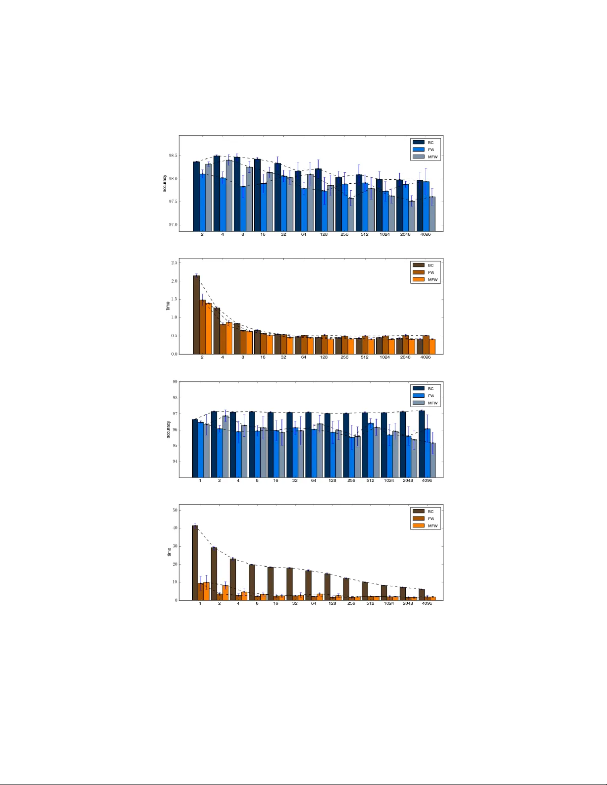
T raining Supp ort V ector Mac hines Using F rank-W olfe Optimization Metho ds Eman uele F randi 1 , Ricardo ˜ Nanculef 2 , Maria Grazia Gasparo 3 , Stefano Lo di 4 , and Claudio Sartori 5 1 Dept. of Science and High T echnology , Univ ersity of Insubria, Italy emanuele.frandi@uninsubria.it 2 Dept. of Informatics, F ederico Santa Mar ´ ıa Universit y , Chile jnancu@inf.utfsm.cl 3 Dept. of Energetics, Universit y of Florence, Italy mariagrazia.gasparo@unifi.it 4,5 Dept. of Electronics, Computer Science and Systems, Universit y of Bologna, Italy { stefano.lodi,claudio.sartori } @unibo.it Abstract T raining a Supp ort V ector Machine (SVM) requires the solution of a quadratic programming problem (QP) whose computational complexity b ecomes prohibitively exp ensive for large scale datasets. T raditional op- timization metho ds cannot b e directly applied in these cases, mainly due to memory restrictions. By adopting a sligh tly different ob jective function and under mild conditions on the kernel used within the mo del, efficien t algorithms to train SVMs hav e b een devised under the name of Core V ector Machines (CVMs). This framework exploits the equiv alence of the resulting learn- ing problem with the task of building a Minimal Enclosing Ball (MEB) problem in a feature space, where data is implicitly embedded by a kernel function. In this pap er, we improv e on the CVM approach by prop osing tw o no vel metho ds to build SVMs based on the F rank-W olfe algorithm, re- cen tly revisited as a fast metho d to approximate the solution of a MEB problem. In contrast to CVMs, our algorithms do not require to compute the solutions of a sequence of increasingly complex QPs and are defined b y using only analytic optimization steps. Exp erimen ts on a large collec- tion of datasets show that our metho ds scale better than CVMs in most cases, sometimes at the price of a slightly low er accuracy . As CVMs, the prop osed metho ds can b e easily extended to machine learning problems other than binary classification. How ever, effectiv e classifiers are also ob- tained using kernels which do not satisfy the condition required b y CVMs and can thus b e used for a wider set of problems. 1 In tro duction Supp ort V ector Machines (SVMs) are curren tly one of the most effectiv e meth- o ds to approac h classification and other mac hine learning problems, improving on more traditional tec hniques like decision trees and neural net works in a n um- b er of applications [16, 33]. SVMs are defined by optimizing a regularized risk functional on the training data, whic h in most cases leads to classifiers with an outstanding generalization performance [39, 33]. This optimization problem is usually form ulated as a large conv ex quadratic programming problem (QP), for which a naiv e implementation requires O ( m 2 ) space and O ( m 3 ) time in the n umber of examples m , complexities that are prohibitively exp ensiv e for large scale problems [33, 37]. Ma jor researc h efforts ha ve been hence directed to w ards scaling up SVM algorithms to large datasets. Due to the t ypically dense structure of the hessian matrices inv olv ed in the QP , traditional optimization methods cannot b e directly applied to train an SVM on large datasets. The problem is usually addressed using an active set metho d where at each iteration only a small num ber of v ariables are allow ed to c hange [32, 18, 30]. In non-linear SVMs problems, this is essen tially equiv alen t to selecting a subset of training examples called a working set [39]. The most prominen t example in this category of methods is Sequen tial Minimal Optimiza- tion (SMO), where only tw o v ariables are selected for optimization each time [8, 30]. The main disadv an tage of these metho ds is that they generally exhibit a slo w lo cal rate of conv ergence, that is, the closer one gets to a solution, the more slowly one approaches that solution. Moreo ver, p erformance results are in practice very sensitive to the size of the active set, the w ay to select the activ e v ariables and other implementation details like the caching strategy used to av oid rep etitiv e computations of the kernel function on which the mo del is based [32] Other attempts to scale up SVM methods consist in adapting interior p oint metho ds to some classes of the SVM QP .[9]. F or large-scale problems ho w- ev er the resulting rank of the k ernel matrix can still be to o high to b e handled efficien tly [37]. The reformulation of the SVM ob jectiv e function as in [12], the use of sampling metho ds to reduce the num b er of v ariables in the problem as in [22] and [20], and the combination of small SVMs using ensem ble me thods as in [29] ha ve also been explored. Lo oking for more efficient metho ds, in [37] a new approach was prop osed: the task of learning the classifier from data can b e transformed to the problem of computing a minimal enclosing b al l (MEB), that is, the ball of smallest radius containing a set of p oin ts. This equiv alence is obtained b y adopting a sligh tly different penalty term in the ob jectiv e function and imp osing some mild conditions on the kernel used by the SVM. Recent adv ances in computational geometry ha ve demonstrated that there are algorithms capable of approximating a MEB with any degree of accuracy  in O (1 / ) iterations indep enden tly of the n umber of points and the dimensionalit y of the space in whic h the ball is built [37]. Adopting one of these algorithms, Tsang and colleagues devised in [37] the Core V ector Machine (CVM), demonstrating that the new metho d compares fa vorably with most traditional SVM soft ware, including for example softw are 2 based on SMO [8, 30]. CVMs start by solving the optimization problem on a small subset of data and then pro ceed iterativ ely . At eac h iteration the algorithm lo oks for a p oin t outside the approximation of the MEB obtained so far. If this p oin t exists, it is added to the previous subset of data to define a larger optimization problem, whic h is solved to obtain a new approximation to the MEB. The pro cess is re- p eated un til no p oin ts outside the curren t appro ximating ball are found within a prescrib ed tolerance. CVMs hence need the resolution of a sequence of opti- mization problems of increasing complexit y using an external n umerical solv er. In order to b e efficient, the solv er should b e able to solv e each problem from a warm-start and to a void the full storage of the corresp onding Gram matrix. Exp erimen ts in Ref. 37 employ to this end a v ariant of the second-order SMO prop osed in [8]. In this pap er, we study tw o no vel algorithms that exploit the formalism of CVMs but do not need the resolution of a sequence of QPs. These algorithms are based on the F rank-W olfe (FW) optimization framework, introduced in [11] and recently studied in [41] and [4] as a metho d to approximate the solution of the MEB problem and other conv ex optimization problems defined on the unit simplex. Both algorithms can b e used to obtain a solution arbitrarily close to the optimum, but at the same time are considerably simpler than CVMs. The key idea is to replace the nested optimization problem to b e solved at each iteration of the CVM approac h b y a linearization of the ob jective function at the curren t feasible solution and an exact line search in the direction obtained from the linearization. Consequen tly , each iteration b ecomes fairly cheaper than a CVM iteration and do es not require an y external numerical solv er. Similar to CVMs, both algorithms incremen tally disco ver the examples which b ecome supp ort vectors in the SVM model, lo oking for the optimal set of w eights in the pro cess. How ever, the second of the prop osed algorithms is also endow ed with the abilit y to explicitly remov e examples from the w orking set used at each iteration of the pro cedure and has thus the potential to compute smaller models. On the theoretical side, b oth algorithms are guaranteed to succeed in O (1 / ) iterations for an arbitrary  > 0. In addition, the second algorithm exhibits an asymptotically linear rate of conv ergence [41]. This research was originally motiv ated b y the use of the MEB framework and computational geometry optimization for the problem of training an SVM. Ho wev er, a ma jor adv antage of the prop osed metho ds ov er the CVM approac h is the p ossibility to employ kernels which do not satisfy the conditions required to obtain the equiv alence b et ween the SVM and MEB optimization problems. F or example, the p opular p olynomial kernel do es not allow the use of CVMs as a training metho d. Since the optimal k ernel for a given application cannot b e sp ecified a priori , the capability of a training metho d to work with an y v alid k ernel function is an imp ortan t feature. Adaptations of the CVM to handle more general k ernels hav e b een recen tly prop osed in [38] but, in contrast, our algorithms can b e used with any Mercer kernel without c hanges to the theory or the implemen tation. The effectiveness of the prop osed metho ds is ev aluated on several data clas- 3 sification sets, most of them already used to show the impro vemen ts of CVMs o ver s econd-order SMO [37]. Our exp erimen tal results suggest that, as long as a minor loss in accuracy is acceptable, our algorithms significantly improv e the actual running times of this algorithm. Statistical tests are conducted to as- sess the significance of these conclusions. In addition, our exp erimen ts confirm that effective classifiers are also obtained with kernels that do not fulfill the conditions required b y CVMs. The article is organized as follows. Section 2 presents a brief ov erview on SVMs and the wa y by which the problem of computing an SVM can b e treated as a MEB problem. Section 3 describ es the CVM approac h. In Section 4 w e in tro duce the prop osed metho ds. Section 5 presents the exp erimen tal setting and our numerical results. Section 6 closes the article with a discussion of the main conclusions of this research. 2 Supp ort V ector Mac hines and the MEB Equiv- alence In this section we presen t an o verview on Supp ort V ector Machines (SVMs), and discuss the conditions under which the problem of building these mo dels can b e treated as a Minimal Enclosing Ball (MEB) problem in a feature space. 2.1 The Pattern Classification Problem Consider a set of training data S = { x i } with x i ∈ X , i ∈ I = { 1 , . . . , m } . The set X , often coinciding with R n , is called the input sp ac e , and each instance is asso ciated with a given category in the set C = { c 1 , c 2 , . . . , c K } . A pattern classification problem consists of inferring from S a prediction mechanism f : X → C ∈ F , termed hypothesis, to asso ciate new instances x ∈ X with the correct category . When K = 2 the problem describ ed ab o ve is called binary classification. This problem can b e addressed by defining a set of candidate mo dels F , a risk functional R l ( S, f ) assessing the ability of f to correctly predict the category of the instances in X , and a pro cedure L by whic h a dataset S is mapp ed to a giv en h yp othesis f = L ( S ) ∈ F ac hieving a lo w risk. In the con text of machine learning, L is called the learning algorithm, F the h yp othesis space and R l ( S, f ) the induction principle [33]. In the rest of this pap er we fo cus on the problem of computing a mo del designed for binary classification problems. The extension of these mo dels to handle multiple categories can b e accomplished in several wa ys. A p ossible approac h corresp onds to use several binary classifiers, separately trained and joined in to a multi-category decision function. W ell known approaches of this t yp e are one-versus-the-rest (OVR, se e [39]), where one classifier is trained to separate eac h class from the rest; one-v ersus-one (O V O, see [19]), where differen t binary SVMs are used to separate each p ossible pair of classes; and DDA G, where one-versus-one classifiers are organized in a directed acyclic graph decision structure [33]. Previous exp erimen ts with SVMs sho w that OV O frequently 4 obtains a b etter p erformance b oth in terms of accuracy and training time [17]. Another type of extension consists in reformulating the optimization problem underlying the metho d to directly address multiple categories. See [6], [23], [28] and [1] for details ab out these methods. 2.2 Linear Classifiers and Kernels Supp ort V ector Machines implement the decision mechanism by using simple linear functions. Since in realistic problems the configuration of the data can b e highly non-linear, SVMs build a linear mo del not in the original space X , but in a high-dimensional dot pro duct fe atur e sp ac e P = lin ( φ ( X )) where the original data is em b edded through the mapping p = φ ( x ) for each x ∈ X . In this space, it is exp ected that an accurate decision function can b e linearly represented. The feature space is related with X b y means of a so called kernel function k : X × X → R , which allo ws to compute dot pro ducts in P directly from the input space. More precisely , for each x i , x j ∈ X , we hav e p T i p j = k ( x i , x j ). The explicit computation of the mapping φ , which w ould b e computationally infeasible, is th us av oided [33]. F or binary classification problems, the most common approach is to asso ciate a p ositiv e lab el y i = +1 to the examples of the first class, and a negativ e lab el y i = − 1 to the examples b elonging to the other class. This approach allo ws the use of real v alued h yp otheses h : P → R , whose output is passed through a sign threshold to yield the classification lab el f ( x ) = sgn( h ( p )) = sgn( h ( φ ( x ))). Since h ( p ) is a linear function in P , the final prediction mechanism takes the form f ( x ) = sgn ( h ( φ ( x ))) = sgn  w T φ ( x ) + b  , (1) with w ∈ P and b ∈ R . This gives a classification rule whose decision b oundary H = { p : w T p + b = 0 } is a hyperplane with normal vector w and p osition parameter b . 2.3 Large Margin Classifiers It should b e noted that a decision function w ell predicting the training data do es not necessarily classify well unseen examples. Hence, minimizing the training error (or empiric al risk ) X i ∈I 1 2 | 1 − y i f ( x i ) | , (2) do es not necessarily imply a small test error. The implementation of an in- duction principle R l ( S, f ) guaranteeing a go o d classification p erformance on new instances of the problem is addressed in SVMs b y building on the con- cept of mar gin ρ . F or a giv en training pair x i , y i , the margin is defined as ρ i = ρ f ( x i , y i ) = y i h ( x i ) = y i  w T φ ( x ) + b  and is exp ected to estimate how reliable the prediction of the mo del on this pattern is. Note that the example x i is misclassified if and only if ρ i < 0. Note also that a large margin of the 5 pattern x i suggests a more robust decision with respect to changes in the param- eters of the decision function f ( x ), whic h are to b e estimated from the training sample [33]. The margin attained by a giv en prediction mechanism on the full training set S is defined as the minim um margin ov er the whole sample, that is ρ = min i ∈I ρ f ( x i , y i ). This implements a measure of the worst classification p erformance on the training set, since ρ i ≥ ρ ∀ i [35]. Under some regularity conditions, a large margin leads to theoretical guarantees of go od p erformance on new decision instances [39]. The decision function maximizing the margin on the training data is thus obtained b y solving maximize w ,b ρ = maximize w ,b min i ρ f ( x i , y i ) . (3) or, equiv alently , maximize w ,b ρ sub ject to ρ i ≥ ρ, i ∈ I . (4) Ho wev er, without some constrain t on the size of w , the solution to this maximin problem do es not exist [35, 14]. On the other hand, ev en if we fix the norm of w , a separating h yp erplane guaran teeing a p ositiv e margin ρ f ( x i , y i ) on each training pattern need not exist. This is the case, for example, if a high noise level causes a large o verlap of the classes. In this case, the hyperplane maximizing (3) p erforms p oorly b ecause the prediction mec hanism is determined en tirely b y misclassified examples and the theoretical results guaranteeing a go od classi- fication accuracy on unseen patterns no longer hold [35]. A standard approach to deal with noisy training patterns is to allo w for the p ossibilit y of examples violating the constraint ρ i ≥ ρ ∀ i and by computing the margin on a subset of training examples. The exact w ay by whic h SVMs address these problems gives rise to sp ecific formulations, called soft-mar gin SVMs. 2.4 Soft-Margin SVM F orm ulations In L 1 -SVMs (see e.g. [5, 33, 14]), degeneracy of problem (3) is addressed by scaling the constrain ts ρ i ≥ ρ as ρ i k w k ≥ ρ and b y adding the constrain t k w k = 1 ρ , so that the problem no w takes the form of the quadratic programming problem minimize w ,b 1 2 k w k 2 sub ject to ρ f ( x i , y i ) ≥ 1 , i ∈ I . (5) Noisy training examples are handled by incorp orating slac k v ariables ξ i ≥ 0 to the constraints in (5) and b y p enalizing them in the ob jectiv e function: minimize w ,b, ξ 1 2 k w k 2 + C X i ∈I ξ i sub ject to ρ f ( x i , y i ) ≥ 1 − ξ i , i ∈ I . (6) 6 This leads to the so called soft-mar gin L 1 -SVM. In this formulation, the pa- rameter C controls the trade-off betw een margin maximization and margin con- strain ts violation. Sev eral other reform ulations of problem (3) can b e found in literature. In particular, in some formulations the tw o–norm of ξ is p enalized instead of the one–norm. In this article, we are particularly interested in the soft mar gin L 2 -SVM prop osed by Lee and Mangasarian in [24]. In this form ulation, the margin constrain ts ρ i ≥ ρ in (3) are preserved, the margin v ariable ρ is explicitly incorp orated in the ob jectiv e function and degeneracy is addressed by penalizing the squared norms of b oth w and b , minimize w ,b,ρ, ξ 1 2 k w k 2 + b 2 + C X i ∈I ξ 2 i ! − ρ sub ject to ρ f ( x i , y i ) ≥ ρ − ξ i , i ∈ I . (7) In practice, L 2 -SVMs and L 1 -SVMs usually obtain a similar classification accuracy in predicting unseen patterns [24, 37]. 2.5 The T arget QP In this paper w e fo cus on the L 2 -SVM model as describ ed abov e. The use of this form ulation is mainly motiv ated by efficiency: b y adopting the slightly mo dified functional of Eqn. 7, we can exploit the framew ork introduced in [37] and solve the learning problem more easily , as we will explain in the next Subsection. As a drawbac k, the constrain ts of problem (7) explicitly dep end on the images p i = φ ( x i ) of the training examples under the mapping φ . In practice, to av oid the explicit computation of the mapping, it is conv enient to derive the W olfe dual of the problem by incorporating m ultipliers α i ≥ 0 , i ∈ I and considering its Lagrangian L ( w , b, ξ , α ) = 1 2 k w k 2 + b 2 + C X i ∈I ξ 2 i ! − ρ − X i ∈I α i ( ρ f ( x i , y i ) − ρ + ξ i ) . (8) F rom the Karush-Kuhn-T uck er conditions for the optimality of (7) with resp ect to the primal v ariables w e ha ve (see [5, 33, 14]): ∂ L ∂ w = 0 ⇔ w = X i ∈I α i y i φ ( x i ) ∂ L ∂ b = 0 ⇔ b = X i ∈I α i y i ∂ L ∂ ξ i = 0 ⇔ ξ i = α i C , i ∈ I ∂ L ∂ ρ = 0 ⇔ X i ∈I α i = 1 . (9) 7 Plugging into the Lagrangian, we hav e L ( w , b, ξ , α ) = − 1 2 X i,j ∈I α i α j y i y j  p T i p j + 1  − 1 2 X i ∈I α 2 i C . (10) By definition of W olfe dual (see [33]), it immediately follo ws that (7) is equiv alent to the follo wing QP: maximize α − X i,j ∈I α i α j  y i y j p T i p j + y i y j + δ ij C  sub ject to X i ∈I α i = 1 , α i ≥ 0 , i ∈ I , (11) where δ ij is equal to 1 if i = j , and 0 otherwise. In contrast to (7), the problem ab o v e dep ends on the training examples images p i = φ ( x i ) only through the dot products p T i p j . By using the k ernel function w e can hence obtain a problem defined entirely on the original data maximize α Θ( α ) := − X i,j ∈I α i α j  y i y j k ( x i , x j ) + y i y j + δ ij C  sub ject to X i ∈I α i = 1 , α i ≥ 0 , i ∈ I . (12) F rom equations (9), w e can also write the decision function (1) in terms of the original training examples as f ( x ) = sgn ( h ( x )), where h ( x ) = w T φ ( x ) + b = X i ∈I α i y i ( k ( x i , x ) + 1) . (13) Note that the decision function ab o ve dep ends only on the subset of training examples for whic h α i 6 = 0. These examples are usually called the supp ort ve ctors of the mo del [33]. The set of supp ort vectors is often considerably smaller than the original training set. 2.6 Computing SVMs as Minimal Enclosing Balls (MEBs) No w w e explain wh y the L 2 -SVM formulation introduced in the previous para- graphs can lead to efficient algorithms to extract SVM classifiers from data. As p oin ted out first in [37] and then generalized in [38], the L 2 -SVM can b e equiv alently formulated as a MEB problem in a certain feature space, that is, as the computation of the ball of smallest radius containing the image of the dataset under a mapping into a dot pro duct space Z . Consider the image of the training set S under a mapping ϕ , that is, ϕ ( S ) = { z i = ϕ ( x i ) : i ∈ I } . Supp ose no w that there exists a kernel function ˜ k such that ˜ k ( x i , x j ) = ϕ ( x i ) T ϕ ( x j ) ∀ i, j ∈ I . Denote the closed ball of center c ∈ Z 8 and radius r ∈ R + as B ( c , r ). The MEB B ( c ∗ , r ∗ ) of ϕ ( S ) can b e defined as the solution of the following optimization problem minimize r 2 , c r 2 sub ject to k z i − c k 2 ≤ r 2 , i ∈ I . (14) By using the k ernel function ˜ k to implement dot pro ducts in Z , the following W olfe dual of the MEB problem is obtained (see [41]): maximize α Φ( α ) := X i ∈I α i ˜ k ( x i , x i ) − X i,j ∈I α i α j ˜ k ( x i , x j ) sub ject to X i ∈I α i = 1 , α i ≥ 0 , i ∈ I . (15) If we denote b y α ∗ the solution of (15), form ulas for the center c ∗ and the squared radius r ∗ 2 of MEB( ϕ ( S )) follow from strong duality: c ∗ = X i ∈I α ∗ i z i , r ∗ 2 = Φ( α ∗ ) = X i,j ∈I α ∗ i α ∗ j ϕ ( x i ) T ϕ ( x j ) . (16) Note that the MEB dep ends only on the subset of p oin ts C for which α ∗ i 6 = 0. It can b e shown that computing the MEB on C ⊂ ϕ ( S ) is equiv alent to computing the MEB on the en tire dataset ϕ ( S ). This set is frequently called a c or eset of ϕ ( S ), a concept w e are going to explore further in the next sections. W e immediately notice a deep similarity b et ween problems (12) and (15), the only difference b eing the presence of a linear term in the ob jectiv e function of the latter. This linear term can b e neglected under mild conditions on the k ernel function ˜ k . Supp ose ˜ k fulfills the following normalization condition: ˜ k ( x i , x i ) = ∆ 2 = constan t . (17) Since P i ∈I α i = 1, the linear term P i ∈I α i ˜ k ( x i , x i ) in (15) b ecomes a con- stan t and can b e ignored when optimizing for α . Equiv alence b et ween the solutions of problems (12) and (15) follows if we set ˜ k to ˜ k ( x i , x j ) = y i y j ( k ( x i , x j ) + 1) + δ ij C , (18) where k is the k ernel function used within the SVM classifier. Therefore, com- puting an SVM for a set of lab elled data S = { x i : i ∈ I } is equiv alent to computing the MEB of the set of feature p oints ϕ ( S ) = { z i = ϕ ( x i ) : i ∈ I } , where the mapping ϕ satisfies the condition ˜ k ( x i , x j ) = ϕ ( x i ) T ϕ ( x j ). A p os- sible implementation of such a mapping is ϕ ( x i ) =  y i φ ( x i ) , y i , 1 √ c e i  , where φ ( x i ) is in turn the mapping asso ciated with the original Mercer kernel k used b y the SVM. Note that the previous equiv alence betw een the MEB and the SVM problems holds if and only if the kernel ˜ k fulfills assumption (17). If, for example, the SVM 9 classifier implements the well-kno wn d -th order p olynomial kernel k ( x i , x j ) =  x T i x j + 1  d , we hav e that ˜ k ( x i , x i ) is no longer a constant, and th us the MEB equiv alence no longer holds. Complex constructions are required to extend the MEB optimization framew ork to SVMs using differen t k ernel functions [38]. 3 B˘ adoiu-Clarkson Algorithm and Core V ector Mac hines Problem (15) is in general a large and dense QP . Obtaining a n umerical solution when m is large is v ery exp ensiv e, no matter whic h kin d of n umerical method one decides to employ . T aking in to accoun t that in practice we can only approximate the solution within a given tolerance, it is conv enien t to mo dify a priori our ob jective: instead of MEB( ϕ ( S )), we can try to compute an approximate MEB in the sense sp ecified by the follo wing definition. Definition 1. L et MEB ( ϕ ( S )) = B ( c ∗ , r ∗ ) and  > 0 b e a given toler anc e. Then, a (1 +  ) –MEB of ϕ ( S ) is a b al l B ( c , r ) such that r ≤ r ∗ and ϕ ( S ) ⊂ B ( c , (1 +  ) r ) . (19) A set C S ⊂ ϕ ( S ) is an  – coreset of ϕ ( S ) if MEB ( C S ) is a (1 +  ) –MEB of ϕ ( S ) . In [2] and [41], algorithms to compute (1 +  )–MEBs that scale ind ep endently of the dimension of Z and the cardinalit y of S hav e been pro vided. In particular, the B˘ adoiu-Clarkson (BC) algorithm describ ed in [2] is able to provide an  – coreset C S of ϕ ( S ) in no more than O (1 / ) iterations. W e denote with C k the coreset appro ximation obtained at the k -th iteration and its MEB as B k = B ( c k , r k ). Starting from a giv en C 0 , at eac h iteration C k +1 is defined as the union of C k and the p oin t of ϕ ( S ) furthest from c k . The algorithm then computes B k +1 and stops if B ( c k +1 , (1 +  ) r k +1 ) contains ϕ ( S ). Exploiting these ideas, Tsang and colleagues introduced in [37] the CVM (Core V ector Machine) for training SVMs supp orting a reduction to a MEB problem. The CVM is describ ed in Algorithm 1, where each C k is identified by the index set I k ⊂ I . The elements included in C k are called the c or e ve ctors . Their role is exactly analogous to that of supp ort vectors in a classical SVM mo del. The expression for the radius r k follo ws easily from (16). Moreov er, it is easy to sho w (see [37]) that step 13 exactly looks for the p oint x i ∗ whose image ϕ ( x i ∗ ) is the furthest from c k . In fact, by using the expressions c k = P j ∈I k α k,j z j and ˜ k ( x i , x i ) = ∆ 2 ∀ i ∈ I , w e obtain: k z i − c k k 2 = ∆ 2 + X j,l ∈I k α k,j α k,l ˜ k ( x j , x l ) − 2 X j ∈I k α k,j ˜ k ( x j , x i ) = ∆ 2 + R k − 2 X j ∈I k α k,j ˜ k ( x j , x i ) . (20) 10 Note how this computation can b e p erformed, by means of k ernel ev alu- ations, in spite of the lack of an explicit representation of c k and z i . Once i ∗ has b een found, it is included in the index set. Finally , the reduced QP corresp onding to the MEB of the new approximate coreset is solved. Algorithm 1 has tw o main sources of computational ov erhead: the computa- tion of the furthest point from c k , which is linear in m , and the solution of the optimization subproblem in step 10. The complexity of the former step can be made constan t and indep enden t of m b y suitable sampling techniques (see [37]), an issue to which we will return later. As regards the optimization step, CVMs adopt a SMO metho d, where only tw o v ariables are selected for optimization at each iteration [8, 30]. It is known that the cost of eac h SMO iteration is not to o high, but the metho d can require a large num b er of iterations in order to satisfy reasonable stopping criteria [30]. Algorithm 1 BC Algorithm for MEB-SVMs: the Core V ector Mac hine Input: S ,  . 1: initialization: compute I 0 and α 0 ; 2: ∆ 2 ← − ˜ k ( x 1 , x 1 ); 3: R 0 ← − P i,j ∈I 0 α 0 ,i α 0 ,j ˜ k ( x i , x j ); 4: r 2 0 ← − ∆ 2 − R 0 ; 5: i ∗ ← − argmax i ∈I γ 2 ( α 0 ; i ) := ∆ 2 + R 0 − 2 P j ∈I 0 α 0 ,j ˜ k ( x j , x i ); 6: k ← − 0; 7: while γ 2 ( α k ; i ∗ ) > (1 +  ) 2 r 2 k do 8: k ← − k + 1; 9: I k ← − I k − 1 ∪ { i ∗ } ; 10: Find α k b y solving the reduced QP problem minimize α ∈ R m R ( α ) := X i,j ∈I k α i α j ˜ k ( x i , x j ) sub ject to X i ∈I k α i = 1 , α i ≥ 0 , i ∈ I k ; (21) 11: R k ← − R ( α k ); 12: r 2 k ← − ∆ 2 − R k ; 13: i ∗ ← − argmax i ∈I γ 2 ( α k ; i ) := ∆ 2 + R k − 2 P j ∈I k α k,j ˜ k ( x j , x i ); 14: end while 15: return I S = I k , α = α k . As regards the initialization, that is, the computation of C 0 and α 0 , a simple c hoice is suggested in [21], which consists in choosing C 0 = { z a , z b } , where z a is an arbitrary p oin t in ϕ ( S ) and z b is the farthest p oin t from z a . Ob viously , in this case the cen ter and radius of B 0 are c 0 = 0 . 5( z a + z b ) and r 0 = 0 . 5 k z a − z b k , resp ectiv ely . That is, we initialize I 0 = { a, b } , α 0 ,a = α 0 ,b = 0 . 5 and α 0 ,i = 0 for i / ∈ I 0 . A more efficient strategy , implemen ted for example in the co de LIBCVM [36], is the following. The pro cedure consists in determining the MEB 11 of a subset P = { z i , i ∈ I P } of p training p oints, where the set of indices I P is randomly chosen and p is small. This MEB is approximated b y running a SMO solv er. In practice, p ' 20 is suggested to b e enough, but one can also try larger initial guesses, as long as SMO can rapidly compute the initial MEB. C 0 is then defined as the set of p oints x i ∈ P gaining a strictly p ositiv e dual weigh t in the pro cess, and I 0 as the set of the corresp onding indices. 4 F rank-W olfe Metho ds for the MEB-SVM Prob- lem 4.1 Ov erview of the F rank-W olfe Algorithm The F r ank-Wolfe algorithm (FW), originally presented in [11], is designed to solv e optimization problems of the form maximize α ∈ Σ f ( α ) , (22) where f ∈ C 1 ( R m ) is a concav e function, and Σ 6 = ∅ a bounded con vex p olyhe- dron. In the case of the MEB dual problem, the ob jective function is quadratic and Σ coincides with the unit simplex. Given the current iterate α k ∈ Σ, a standard F rank-W olfe iteration consists in the following steps: 1. Find a p oin t u k ∈ Σ maximizing the lo cal linear approximation ψ k ( u ) := f ( α k ) + ( u − α k ) T ∇ f ( α k ), and define d F W k = u k − α k . 2. Perform a line-search λ k = argmax λ ∈ [0 , 1] f ( α k + λ d F W k ). 3. Up date the iterate by α k +1 = α k + λ k d F W k = (1 − λ k ) α k + λ k u k . (23) The algorithm is usually stopp ed when the ob jective function is sufficien tly close to its optimal v alue, according to a suitable pro ximity measure [13]. Since ψ k ( u ) is a linear function and Σ is a bounded p olyhedron, the search directions d F W k are alwa ys directed tow ards an extreme p oint of Σ. That is, u k is a vertex of the feasible set. The constrain t λ k ∈ [0 , 1] ensures feasibility at each iteration. It is easy to show that in the case of the MEB problem u k = e i ∗ , where e i denotes the i -th v ector of the canonical basis, and i ∗ is the index corresp onding to the largest comp onen t of ∇ f ( α k ) [41]. The up dating step therefore assumes the form α k +1 = (1 − λ k ) α k + λ k e i ∗ . (24) It can b e prov ed that the ab o ve pro cedure con verges globally [13]. As a dra wback, ho wev er, it often exhibits a tendency to stagnate near a solution. In tuitively , supp ose that solutions α ∗ of (22) lie on the b oundary of Σ (this is 12 often true in practice, and holds in particular for the MEB problem). In this case, as α k gets close to a solution α ∗ , the directions d F W k b ecome more and more orthogonal to ∇ f ( α k ). As a consequence, α k p ossibly nev er reac hes the face of Σ containing α ∗ , resulting in a sublinear conv ergence rate [13]. 4.2 The Mo dified F rank-W olfe Algorithm W e no w describe an improv ement ov er the general F rank-W olfe pro cedure, whic h w as first prop osed in [40] and later detailed in [13]. This improv ement can b e quan tified in terms of the rate of con vergence of the algorithm and thus of the n umber of iterations in whic h it can b e exp ected to fulfill the stopping conditions. In practice, the tendency of FW to stagnate near a solution can lead to later iterations w asting computational resources while making minimal progress to wards the optimal function v alue. It would thus b e desirable to obtain a stronger result on the conv ergence rate, which guarantees that the sp eed of the algorithm do es not deteriorate when approaching a solution. This paragraph describ es a technique geared precisely tow ards this aim. Essen tially , the previous algorithm is enhanced by introducing alternative searc h directions known as away steps . The basic idea is that, instead of mo ving to wards the v ertex of Σ maximizing a linear approximation ψ k of f in α k , w e can mo ve a wa y from the vertex minimizing ψ k . At each iteration, a choice b etw een these t wo options is made by choosing the b est ascent direction. The whole pro cedure, known as Mo difie d F r ank-Wolfe algorithm (MFW), can be sk etched as follows: 1. Find u k ∈ Σ and define d F W k as in the standard FW algorithm. 2. Find v k ∈ Σ b y minimizing ψ k ( v ), s.t. v j = 0 if α k,j = 0. Define d A k = α k − v k . 3. If ∇ f ( α k ) T d F W k ≥ ∇ f ( α k ) T d A k , then d k = d F W k , else d k = d A k . 4. Perform a line-searc h λ k = argmax λ ∈ [0 , ¯ λ ] f ( α k + λ d k ), where ¯ λ = 1 if d k = d F W k and ¯ λ = max λ ≥ 0  λ | α k + λ d A k ∈ Σ  . 5. Up date the iterate by α k +1 = α k + λ k d k = ( (1 − λ k ) α k + λ k u k if d k = d F W k (1 + λ k ) α k − λ k v k if d k = d A k . (25) It is easy to sho w that b oth d F W k and d A k are feasible ascen t directions, unless α k is already a stationary p oin t. In the case of the MEB problem, step 2 corresp onds to finding the basis v ector e j ∗ corresp onding to the smaller comp onen t of ∇ f ( α k ) [41]. Note that a face of Σ of low er dimensionalit y is reac hed whenev er an a wa y step with maximal stepsize ¯ λ is p erformed. Imp osing the constraint in step 2 is tantamoun t to 13 ruling out a wa y steps with zero stepsize. That is, an a wa y step from e j cannot b e tak en if α k,j is already zero. In [13] linear conv ergence of f ( α k ) to f ( α ∗ ) was prov ed, assuming Lipschitz con tinuit y of ∇ f , strong concavit y of f , and strict complementarit y at the so- lution. In [41], a pro of of the same result was pro vided for the MEB problem, under weak er assumptions. It is imp ortan t to note that such assumptions are in particular satisfied for the MEB form ulation of the L 2 -SVM, and that as such the aforementioned linear con vergence prop ert y holds for all problems consid- ered in this pap er. In particular, uniqueness of the solution, which is implied if w e ask for strong (or just strict) conca vity , is not required. The gist is essen tially that, in a small neighborho o d of a solution α ∗ , MFW is forced to p erform aw ay steps un til the face of Σ containing α ∗ is reac hed, which happ ens after a finite n umber of iterations. Starting from that p oin t, the algorithm b ehav es as an unconstrained optimization metho d, and it can b e prov ed that f ( α k ) conv erges to f ( α ∗ ) linearly [13]. 4.3 The FW and MFW Algorithms for MEB-SVMs If FW metho d is applied to the MEB dual problem, the structure of the ob jectiv e function Φ( α ) can b e exploited in order to obtain explicit form ulas for steps 1 and 2 of the generic pro cedure. Indeed, the comp onen ts of ∇ Φ( α k ) are given b y ∇ Φ( α k ) i = k z i k 2 − 2 X j ∈I α k,j z T i z j = k z i k 2 − 2 z T i c k , (26) where c k = X j ∈I α k,j z j , (27) and therefore, since k c k k 2 do es not dep end on i , i ∗ = argmax i ∈I ∇ Φ( α k ) i = argmax i ∈I k z i − c k k 2 . (28) In practice, step 1 selects the index of the input p oint maximizing the distance from c k , exactly as done in the CVM pro cedure. Computation of distances can b e carried out as in CVMs, using (20). As regards step 2, it can be sho wn (see [4, 41]) that λ k = 1 2  1 − r 2 k k z i ∗ − c k k 2  , (29) where r 2 k = Φ( α k ) . (30) By comparing (27) and (30) with (16), we argue that, as in the BC algorithm, a ball B k = B ( c k , r k ) is iden tified at each iteration. The whole pro cedure is sketc hed in Algorithm 2, where at each iteration we asso ciate to α k the index set I k = { i ∈ I : α k,i > 0 } . 14 Algorithm 2 F rank-W olfe Algorithm for MEB-SVMs Input: S ,  . 1: initialization: compute I 0 and α 0 ; 2: ∆ 2 ← − ˜ k ( x 1 , x 1 ); 3: R 0 ← − P i,j ∈I 0 α 0 ,i α 0 ,j ˜ k ( x i , x j ); 4: r 2 0 ← − ∆ 2 − R 0 ; 5: i ∗ ← − argmax i ∈I γ 2 ( α 0 ; i ) := ∆ 2 + R 0 − 2 P j ∈I 0 α 0 ,j ˜ k ( x j , x i ); 6: δ 0 ← − γ 2 ( α 0 ; i ∗ ) r 2 0 − 1; 7: k ← − 0; 8: while δ k > (1 +  ) 2 − 1 do 9: λ k ← − 1 2  1 − r 2 k γ 2 ( α k ; i ∗ )  ; 10: k ← − k + 1; 11: α k ← − (1 − λ k − 1 ) α k − 1 + λ k − 1 e i ∗ ; 12: I k ← − { i ∈ I : α k,i > 0 } ; 13: R k ← − P i,j ∈I k α k,i α k,j ˜ k ( x i , x j ); 14: r 2 k ← − r 2 k − 1  1 + δ 2 k − 1 4(1+ δ k − 1 )  ; 15: i ∗ ← − argmax i ∈I γ 2 ( α k ; i ) := ∆ 2 + R k − 2 P j ∈I k α k,j ˜ k ( x j , x i ); 16: δ k ← − γ 2 ( α k ; i ∗ ) r 2 k − 1; 17: end while 18: return I S = I k , α = α k . As regards the initialization, α 0 and I 0 can be defined exactly as in the CVM pro cedure. A t subsequent iterations, the formula to up date I k immediately follo ws from the up dating (24) for α k ; indeed, the indices of the strictly p ositiv e comp onen ts of α k +1 are the same of α k , plus i ∗ if α k,i ∗ = 0 (which means that z i ∗ w as not already included in the current coreset). The introduction of the sequence {I k } in Algorithm 2 makes it evident that structure and output of Algorithm 1 are preserved. The up dating formula used in step 14 appears in [41]. It is easy to see that it is equiv alent to (30) and computationally more con venien t. In [41], it has b een prov ed that { r 2 k } is a monotonically increasing sequence with r ∗ 2 as an upp er b ound. Therefore, since the same stopping criterion of the BC algorithm is used, I S iden tifies an  –coreset C S of ϕ ( S ), and the last B k is a (1 +  )–MEB of ϕ ( S ). Ho wev er, the MEB-approximating pro cedure differs from that of BC in that the v alue of r 2 k is not equal to the squared radius of MEB( C k ), but tends to the correct v alue as α k gets near the optimal solution (see Fig. 1). The deriv ation of the MFW metho d applied to the MEB-SVM problem can b e written down along the same lines. F ollowing the presentation in [41], we describ e the detailed pro cedure in Algorithm 3. By now, it should b e apparent that j ∗ is the index identifying the p oin t furthest from c k , and that it corresponds to the smallest component of ∇ Φ( α k ). 15 z i ∗ B k +1 = MEB( C k +1 ) [BC] B k +1 [FW] MEB( C k ) c k Figure 1: Approximating balls computed by algorithms BC and FW. That is, in Algorithm 3 we consider p erforming aw ay steps in whic h the weigh t of the nearest p oin t to the current cen ter is reduced. Of course, since the weigh t of a p oin t is not allow ed to drop b elow zero, the search for j ∗ is p erformed on I k only . Again, the optimal stepsize can b e determined in closed form [41]. In particular, it is easy to see that the expression in step 19 corresp onds to λ k = argmax λ ∈  0 , α k,j ∗ 1 − α k,j ∗  Φ((1 + λ ) α k − λ e j ∗ ) , (31) where the upp er b ound on the interv al preserves dual feasibility . This kind of step has an intuitiv e geometrical meaning: if we consider a solution α ∗ of the MEB problem, it is known that nonzero comp onen ts of α ∗ corresp ond to p oin ts lying on the b oundary of the exact MEB. Therefore, it mak es sense to try to remo ve from the mo del p oints that lie near the center (i.e. far from the b oundary of the ball). When an aw ay step is p erformed, if λ k is chosen as the suprem um of the search interv al, we get α k +1 ,j ∗ = 0 and the corresp onding example is remov ed from the current coreset ( dr op step ). Moreo ver, it’s not hard to see that step 11 chooses to p erform an aw a y step whenev er ∇ Φ( α k ) T d A k > ∇ Φ( α k ) T d F W k . (32) That is, the choice b et ween FW and aw ay steps is done by choosing the b est ascen t direction, exactly as required b y the MFW pro cedure. Here d F W k = ( e i ∗ − α k ) and d A k = ( α k − e j ∗ ) denote the search directions of FW and aw ay steps, resp ectiv ely . Finally , step 20 shows that, just as with standard FW steps, after p erforming an a wa y step we can use an analytical form ula to up date r 2 k . This expression follows easily by writing the ob jectiv e function Φ( α ) for α = (1 + λ ) α k − λ e j ∗ . In Fig. 2, we try to give a geometrical insight on the difference b et ween FW and aw ay steps in terms of search directions. 16 Algorithm 3 Mo dified F rank-W olfe Algorithm for MEB-SVMs Input: S ,  . 1: initialization: compute I 0 and α 0 ; 2: ∆ 2 ← − ˜ k ( x 1 , x 1 ); 3: R 0 ← − P i,j ∈I 0 α 0 ,i α 0 ,j ˜ k ( x i , x j ); 4: r 2 0 ← − ∆ 2 − R 0 ; 5: i ∗ ← − argmax i ∈I γ 2 ( α 0 ; i ) := ∆ 2 + R 0 − 2 P j ∈I 0 α 0 ,j ˜ k ( x j , x i ); 6: j ∗ ← − argmin j ∈I 0 γ 2 ( α 0 ; j ); 7: δ 0+ ← − γ 2 ( α 0 ; i ∗ ) r 2 k − 1; 8: δ 0 − ← − 1 − γ 2 ( α 0 ; j ∗ ) r 2 k ; 9: k ← − 0; 10: while δ k + > (1 +  ) 2 − 1 do 11: if δ k + ≥ δ k − then 12: λ k ← − 1 2  1 − r 2 k γ 2 ( α k ; i ∗ )  ; 13: k ← − k + 1; 14: α k ← − (1 − λ k − 1 ) α k − 1 + λ k − 1 e i ∗ ; 15: r 2 k ← − r 2 k − 1  1 + δ 2 k − 1+ 4(1+ δ k − 1+ )  ; 16: else 17: λ k ← − min n δ k − 2(1 − δ k − ) , α k,j ∗ 1 − α k,j ∗ o ; 18: k ← − k + 1; 19: α k ← − (1 + λ k − 1 ) α k − 1 − λ k − 1 e j ∗ ; 20: r 2 k ← − (1 + λ k − 1 ) r 2 k − 1 − λ k − 1 (1 + λ k − 1 )( δ k − 1 − − 1) r 2 k − 1 ; 21: end if 22: I k ← − { i ∈ I : α k,i > 0 } ; 23: R k ← − P i,j ∈I k α k,i α k,j ˜ k ( x i , x j ); 24: i ∗ ← − argmax i ∈I γ 2 ( α k ; i ) := ∆ 2 + R k − 2 P j ∈I k α k,j ˜ k ( x j , x i ); 25: j ∗ ← − argmin j ∈I k γ 2 ( α k ; j ); 26: δ k + ← − γ 2 ( α k ; i ∗ ) r 2 k − 1; 27: δ k − ← − 1 − γ 2 ( α k ; j ∗ ) r 2 k ; 28: end while 29: return I S = I k , α = α k . W e previously hinted at the linear con vergence prop erties of MFW. This result can no w b e stated more precisely [41]. Prop osition 1. A t e ach iter ation of the MFW algorithm, we have: Φ( α ) − Φ( α k +1 ) Φ( α ) − Φ( α k ) ≤ M , (33) wher e M ≤ 1 − 1 36 mβ d S , β is a c onstant and d S = diam( S ) 2 . 17 e i ∗ e j ∗ α k d F W k d A k α F W k +1 α A k +1 Figure 2: A sketc h of the searc h directions used by FW and MFW. Substan tially , as shown in the conv ergence analysis of [13], there exists a p oin t in the optimization path of the MFW algorithm after whic h only aw ay steps are p erformed. That is, the algorithm only needs to remov e useless exam- ples to correctly identify the optimal supp ort vector set. F rom this stage on, the algorithm con verges linearly to the optim um v alue of the ob jective function. In contrast, the standard FW algorithm do es not possess the explicit ability to eliminate spurious patterns from the index set, and tends to slow down when getting near the solution. 4.4 Bey ond Normalized Kernels The methods studied in this pap er w ere originally motiv ated b y recent adv ances in computational geometry that led to efficient algorithms to address the MEB problem [41]. Ho wev er, a ma jor adv antage of the prop osed metho ds, ov er e.g. the CVM approach, is that b oth the theory and the implementation of our algorithms can b e applied without changes to train SVMs using kernels which do not satisfy condition (17), imp osed to obtain the equiv alence b et ween the MEB problem (15) and the SVM optimization problem (12). Both the FW and MFW metho ds were designed to maximize an y differen- tiable concav e function f ( α ) in a b ounded conv ex p olyhedron. The ob jective function in the SVM problem (12) is conca ve and the set of constrain ts coincides with the unit simplex. The prop osed metho ds can thus b e applied directly to solv e (12) without regard to (15). Theoretical results such as the global conv er- gence of algorithms still hold. In addition, since strict complemen tarity usually holds for SVM problems, results in [13] imply that MFW still conv erges linearly 18 to the optimum. Note also that the constant ∆ 2 , which makes the difference b et w een (15) and (12) for normalized kernels, can still be added to the ob jective function of (12) in the case of non-normalized k ernels, since it is simply ignored when optimizing for α . An implemen tation designed to handle normalized ker- nels can th us b e directly used with an y Mercer kernel. It is apparent that the geometrical in terpretation underlying Algorithms 2 and 3 needs to b e reformulated if the SVM problem is no longer equiv alent to the problem of computing a MEB. Ho wev er, it is easy to show that the search direction of the FW pro cedure at iteration k is still e i ∗ where the index i ∗ corresp onds to the largest comp onen t of ∇ f ( α k ). Similarly , the aw ay direction explored by MFW at iterate k is still e j ∗ where the index j ∗ corresp onds to the smallest component of ∇ f ( α k ). The set of constrain ts in problem (12) coincides with that of (15). In addition, any approximate solution α k pro duced by the prop osed algorithms is feasible. Thus, the sequence f ( α k ) is strictly increasing and con verges from below to the optim um f ( α ∗ ). It is not immediately evident, ho wev er, whether the stopping condition used within our algorithms guarantees the metho d to find a solution in a neighborho o d of the optimum α ∗ k . W e now sho w that this is indeed the case. F or simplicity of notation, it is conv enient to write explicitly the target QP of MEB-SVMs in matrix form: maximize α g ( α ) := ∆ 2 − α ˜ K α = ∆ 2 − k c k 2 sub ject to e T α = 1 , α ≥ 0 , (34) where ˜ K is the matrix of en tries ˜ k ij = ϕ ( x i ) T ϕ ( x j ) = y i y j k ( x i , x j ) + y i y j + δ ij C , c = Z α , and Z is the matrix whose columns are the feature v ectors z i = ϕ ( x i ). Note that K = Z T Z . When k is a normalized kernel, we get Φ( α ) = g ( α ). F or non-normalized kernels, instead, ∆ 2 can b e viewed as an arbitrary constant added to the SVM ob jective function in (12), Θ( α ) = − α ˜ K α . That is, we can alw ays think of g ( α ) as the ob jectiv e function when solving (12). It is not hard to see that the stopping condition used in Algorithms 2 and 3 can b e written as follows: δ k + ≤ (1 +  ) 2 − 1 ⇐ ⇒ k z i ∗ − c k k 2 ≤ (1 +  ) 2 r 2 k ⇐ ⇒ ∆ 2 − 2 z T i ∗ c k + k c k k 2 ≤ (1 +  ) 2 r 2 k . (35) Since by construction r 2 k = ∆ 2 − k c k k 2 , we get ∆ 2 − 2 z T i ∗ c k + k c k k 2 ≤ (1 + 2  +  2 )  ∆ 2 − k c k k 2  ⇐ ⇒ ∆ 2 − 2 z T i ∗ c k + k c k k 2 ≤ (1 + ε )  ∆ 2 − k c k k 2  ⇐ ⇒ ∆ 2 − 2 z T i ∗ c k + k c k k 2 ≤ ∆ 2 − k c k k 2 + εg ( α k ) ⇐ ⇒ − 2 z T i ∗ c k + 2 k c k k 2 ≤ εg ( α k ) , (36) with ε = 2  +  2 = O (  ). No w, since ∇ g ( α k ) = − 2 K α k = − 2 Z T c k , w e ha ve that ∇ g ( α k ) i ∗ = − 2 z T i ∗ c k . In addition, α T k ∇ g ( α k ) = − 2 α T k K α k = 19 − 2 α T k Z T Z α k = − 2 c T k c k = − 2 k c k k 2 . Th us, the stopping condition for b oth algorithms is equiv alent to ∇ g ( α k ) i ∗ − α T k ∇ g ( α k ) ≤ εg ( α k ) . (37) On the other hand, since the ob jective function g ( α ) is conca ve and differen- tiable, g ( α ∗ ) ≤ g ( α k ) + ( α ∗ − α k ) T ∇ g ( α k ) . (38) In addition, e T α ∗ = 1 and thus α ∗ T ∇ g ( α k ) ≤ max i ∈I ∇ g ( α k ) i = ∇ g ( α k ) i ∗ . Therefore, g ( α ∗ ) ≤ g ( α k ) + α ∗ T ∇ g ( α k ) − α T k ∇ g ( α k ) ≤ g ( α k ) + ∇ g ( α k ) i ∗ − α T k ∇ g ( α k ) . (39) In virtue of (37) and (39), we obtain that g ( α ∗ ) ≤ g ( α k ) + εg ( α k ) = (1 + ε ) g ( α k ) . (40) Finally , from the feasibilit y of α k , we hav e g ( α k ) ≤ g ( α ∗ ). Therefore, (1 − ε ) g ( α ∗ ) ≤ g ( α k ) ≤ g ( α ∗ ) , (41) that is, Algorithms 2 and 3 stop with an ob jective function v alue g ( α k ) in a left neigh b orho od of radius g ( α ∗ ) ε = g ( α ∗ )(2  +  2 ) = O (  ) around the optimum, ev en if the target problem (12) is not equiv alent to a MEB problem. 5 Exp erimen ts W e test all the classifications metho ds discussed ab o ve on sev eral classification problems. Our aim is to show that, as long as a minor loss in accuracy is acceptable, F rank-W olfe based methods are able to build L 2 -SVM classifiers in a considerably smaller time compared to CVMs, whic h in turn ha ve been prov en in [37] to b e faster than most traditional SVM softw are. This is esp ecially eviden t on large-scale problems, where the capability to construct a classifier in a significantly reduced amoun t of time ma y b e most useful. 5.1 Organization of this Section After discussing several implementation issues we compare the p erformance of the studied algorithms on several classical datasets. Our exp erimen ts include scalabilit y tests on tw o different collections of problems of increasing size, which assess the capability of F rank-W olfe based metho ds to efficiently solv e problems of increasingly large size. These results can b e found in Subsecs. 5.3 and 5.4. In Subsection 5.5 w e present additional exp erimen ts on the set of problems studied in [10]. The statistical significance of the results presented so far is analyzed in section 5.6. A separate test is then p erformed in Subsection 5.7 to study the influence of the p enalt y parameter C on each training algorithm. Finally , 20 in Subsection 5.8 we present some exp erimen ts sho wing the capabilit y of FW and MFW methods to handle a wider family of kernel function with respect to CVMs. W e highligh t that the purp ose of that paragraph is not to improv e the accuracy or the training time of the algorithms. A detailed commentary on the obtained results, whic h summarizes and expands on our conclusions, closes the section in Subsection 5.9. 5.2 Datasets and Implemen tation Issues As w e detail b elo w, all the datasets used in this section ha ve b een widely used in the literature. They were selected to cov er a large v ariety with resp ect to the n umber of instances, num b er of dimensions and num b er of classes. In most of the cases, the training and testing sets are standard (precomputed for b enc h- marking) and can be obtained from public repositories lik e [3], [15], or others w e indicate in the dataset descriptions. The exceptions to this rule are the datasets P endigits and KDD99-10p c . In these cases, the testing set was obtained b y random sampling from the original collection a 20% of the items. All the examples not selected as test instances were employ ed for training. F or each problem, we sp ecify , in T ab. 1, the num b er m of training p oin ts, the input space dimension n , and the num b er of classes K . W e indicate by t the n umber of examples in the test set , which is used to ev aluate the accuracy of the classifiers but never employ ed for training or parameter tuning. In the case of multi-category classification problems, we adopted the one-versus-one approac h (OV O), which is the metho d used in [37] to extend CVMs b ey ond binary classification and that usually obtains the b est p erformance both in terms of accuracy and training time according to [17]. Hence, for these cases we also rep ort the size m max of the largest binary subproblem and the size m min of the smallest binary subproblem in the OV O decomp osition. Here follo w some brief descriptions of the pattern recognition problems un- derlying each dataset, tak en from their resp ectiv e sources. • USPS , USPS-Ext - The USPS dataset is a classic handwritten digits recognition problem, where the patterns are 16 × 16 images from United States Postal Service en velopes. The extended version USPS-Ext first app eared in [37] to sho w the large-scale capabilities of CVMs. The original v ersion can b e downloaded from [3] and the extended one from [36]. • Pendigits - Another digit recognition dataset, created by exp erimen tally collecting samples from a total of 44 writers with a tablet and a stylus. This dataset can b e obtained from [15]. • Letter - An Optical Character Recognition (OCR) problem. The ob jec- tiv e is to identify e ac h of a large num b er of black-and-white rectangular pixel displays as one of the 26 capital letters in the English alphab et. The files can b e obtained from [3]. • Protein - A bioinformatics problem regarding protein structure predic- tion. This dataset can be download from [3]. 21 Dataset m t K m max m min n USPS 7291 2007 10 2199 1098 256 P endigits 7494 3498 10 1560 1438 16 Letter 15000 5000 26 1213 1081 16 Protein 17766 6621 3 13701 9568 357 Sh uttle 43500 14500 7 40856 17 9 IJCNN 49990 91701 2 49990 49990 22 MNIST 60000 10000 10 13007 11263 780 USPS-Ext 266079 75383 2 266079 266079 676 KDD99-10p c 395216 98805 5 390901 976 127 KDD99-F ull 4898431 311029 2 4898431 4898431 127 Reuters 7770 3299 2 7770 7770 8315 Adult a1a 1605 30956 2 1605 1605 123 Adult a2a 2265 30296 2 2265 2265 123 Adult a3a 3185 29376 2 3185 3185 123 Adult a4a 4781 27780 2 4781 4781 123 Adult a5a 6414 26147 2 6414 6414 123 Adult a6a 11220 21341 2 11220 11220 123 Adult a7a 16100 16461 2 16100 16100 123 W eb w1a 2477 47272 2 2477 2477 300 W eb w2a 3470 46279 2 3470 3470 300 W eb w3a 4912 44837 2 4912 4912 300 W eb w4a 7366 42383 2 7366 7366 300 W eb w5a 9888 39861 2 9888 9888 300 W eb w6a 17188 32561 2 17188 17188 300 W eb w7a 24692 25057 2 24692 24692 300 W eb w8a 49749 14951 2 49749 49749 300 T able 1: F eatures of the selected datasets. • Shuttle - This is a dataset in the Statlog collection, originated from NASA and concerning the p osition of radiators within the Space Sh uttle [27]. The dataset can b e obtained from [15] or [36]. • IJCNN - A dataset from the 2001 neural net work comp etition of the In ternational Joint Conference on Neural Netw orks. W e obtained this dataset from [37]. • MNIST - Another classic handwritten digit recognition problem, this time coming from National Institute of Standards (NIST) data. The dataset can b e obtained from [36]. • KDD99-10p c , KDD99-F ull - This is a dataset used in the 1999 Knowl- edge Discov ery and Data Mining Cup. The data are connection records for a netw ork, obtained b y simulating a wide v ariety of normal accesses and intrusions on a military net work. The problem is to detect different t yp es of accesses on the netw ork with the aim of identifying fraudulent ones. The 10pc version is a randomly selected 10% of the whole data. 22 • Reuters - A text categorization problem built from a collection of do cu- men ts that app eared on Reuters newswire in 1987. The do cumen ts w ere assem bled and indexed with categories. The binary version used in this pap er (relev ant versus non-relev ant do cumen ts) w as obtained from [36]. • Adult a1a-a8a - A series of problems derived from a dataset extracted from the 1994 US Census database. The original aim w as to predict whether an individual’s income exceeded 50000US$/year, based on p er- sonal data. All the instances of this collection can b e do wnloaded from [36]. • W eb w1a-w8a - A series of problems extracted from a web classification task dataset, first app eared in Platt’s pap er on Sequen tial Minimal Opti- mization for training SVMs [30]. All the instances of this collection can b e do wnloaded from [36]. 5.2.1 SVM P arameters F or the experiments presented in Subsection 5.3 to Subsection 5.7, SVMs w ere trained using a RBF k ernel k ( x 1 , x 2 ) = exp( −k x 1 − x 2 k 2 / 2 σ 2 ). The reason for this c hoice is that this k ernel is the best-known in the family of k ernels admitted b y CVMs and it is frequently used in practice [37]. In particular, this is the c hoice for the large set of exp erimen ts presented in [37] to demonstrate the adv antage of this framework on other SVM softw are. How ever, in Subsection 5.8 we presen t some results showing the capability of FW and MFW metho ds to handle a p olynomial kernel, which do es not satisfy the conditions required b y CVMs. F or the relatively small datasets Pendigits and USPS , parameter σ 2 w as determined together with parameter C of SVMs using 10-fold cross-v alidation on the logarithmic grid [2 − 15 , 2 5 ] × [2 − 5 , 2 15 ], where the first collection of v alues corresp ond to parameter σ 2 and the second to parameter C . F or the large-scale datasets, σ 2 w as determined using the default metho d employ ed b y CVMs in [37], that is, it was set to the a verage squared distance among training patterns. P arameter C w as determined on the logarithmic grid [2 0 , 2 12 ] using a v alidation set consisting in a randomly computed 30% fraction of the training set. W e stress that the aim of this pap er is not to determine an optimal v alue of the parameters by fine-tuning each algorithm on the test problems to seek for the b est possible accuracy . As our in tent is to compare the p erformance of the presen ted metho ds and analyze their b ehavior in a manner consistent with our theoretical analysis, it is necessary to p erform the exp erimen ts under the same conditions on a given dataset. That is to say , the optimization problem to b e solv ed should b e the same for each algorithm. F or this reason, we delib erately a voided using different training parameters when comparing different metho ds. Sp ecifically , parameters σ 2 and C w ere tuned using the CVM metho d and the obtained v alues were used for all the algorithms discussed in this paper (CVM, FW and MFW). 23 F urthermore, since the v alue of parameter C can hav e a significant influence on the running times, we devote a sp ecific subsection to ev aluate the effect of this parameter on the different training algorithms. 5.2.2 MEB Initialization and Parameters As regards the initialization of the CVM, FW and MFW metho ds, that is, the computation of I 0 and α 0 in Algorithms 1, 2 and 3, we adopted the random MEB metho d describ ed in the previous sections, using p = 20 p oin ts. As suggested in [37], we used  = 10 − 6 with all the algorithms. 5.2.3 Random Sampling T echniques Computing i ∗ , i.e. ev aluating (20) for all of the m training p oints, requires a num b er of k ernel ev aluations of order O ( q 2 k + mq k ) = O ( mq k ), where q k is the cardinality of I k . If m is very large, this complexity can quic kly b ecome unacceptable, ruling out the p ossibilit y to solve large scale classification prob- lems in a reasonable time. A sampling technique, called pr ob abilistic sp e e dup , w as prop osed in [34] to ov ercome this obstacle. In practice, the distance (20) is computed just on a random subset ϕ ( S 0 ) ⊂ ϕ ( S ), where S 0 is identified by an index set I 0 of small constant cardinality r . The ov erall complexity is thereb y reduced to order O ( q 2 k + q k ) = O ( q 2 k ), a ma jor impro vemen t on the previous estimate, since we generally hav e q k  m . The main result this technique relies on is the following [33]. Theorem 1. L et D := { d 1 , . . . , d m } ⊂ R b e a set of c ar dinality m , and let D 0 ⊂ S b e a r andom subset of size r . Then the pr ob ability that max D 0 is gr e ater or e qual than ˜ m elements of D is at le ast 1 − ( ˜ m m ) r . F or example, if r = 59 and ˜ m = 0 . 95 m ,then with probability at least 0 . 95 the p oint in ϕ ( S 0 ) farthest from the center lies among the 5% of the farthest p oin ts in the whole set ϕ ( S ). This is the choice originally made in [37] and used in [10] to test the CVM and FW algorithms. 5.2.4 Cac hing W e also adopted the LRR caching strategy designed in [36] for CVMs to a void the computation of recently used k ernel v alues. 5.2.5 Computational En vironment The exp erimen ts were conducted on a p ersonal computer with a 2.66GHz Quad Core CPU and 4 GB of RAM, running 64bit GNU/Linux (Ubuntu 10.10). The algorithms were implemen ted based on the (C++) source co de av ailable at [36]. 24 5.3 Scalabilit y Experiments on the W eb Dataset Collec- tion In Fig. 3, w e rep ort some results concerning accuracies , training times, sp eed- ups and supp ort vector set sizes obtained in the W eb datasets. The series is monotonically increasing in the num b er of training patterns, whic h grows appro ximately as m i = 1 . 4 i m 0 , i = 1 , . . . , 8, where m 0 is the num b er of training patterns in the first dataset [30]. The sp eed-up of the FW metho d with resp ect to CVMs is measured as s = t 0 /t 1 where t 0 is the training time of the CVM algorithm and t 1 is the training time of the FW metho d, b oth measured in seconds. Similarly , the sp eed-up of the MFW metho d with resp ect to CVMs is measured as s = t 0 /t 2 where t 2 is the training time of the MFW method. As depicted in Fig. 3 the prop osed metho ds are slightly less accurate than CVMs. The training time, in contrast, scales considerably b etter for our meth- o ds as the num b er of training patterns increases. The sp eed-ups are actually alw ays greater than 1, which shows that the FW and MFW metho ds indeed build classifiers faster than CVMs. More imp ortan tly , the sp eed-up is mono- tonically increasing, ranging from 12 times faster up to 107 times faster in the case of the FW algorithm and from 2 times faster up to almost 10 times faster in the case of the MFW metho d. This suggests that the improv ements of the prop osed metho d ov er CVMs becomes more and more significan t as the size of the training set grows. 5.4 Scalabilit y Exp erimen ts on the Adult Dataset Collec- tion Fig. 4 depicts accuracies and sp eed-ups obtained in the Adult datasets. Lik e the W eb datasets, this collection was created with the purp ose of analyzing the scalability of SVM metho ds and the num b er of training patterns grows appro ximately with the same rate [30]. The sp eed-up of the FW and MFW metho ds is computed as in the previous section. Results obtained in this exp erimen t confirm that the proposed methods tend to b e faster than CVMs as the dataset gro ws. CVMs are actually faster than FW just in tw o cases, corresp onding to the smallest versions of the sequence. MFW how ever runs alwa ys faster than CVMs, reaching a sp eed-up of 15 × in the fifth version of the series. The sp eed-ups obtained b y the FW metho d are in this exp erimen t more mo derate than in the W eb collection. How ever, most of the time FW exhibits also better test accuracies than CVMs. Finally , the MFW algorithm is not only faster but also as accurate as CVMs on this classification problem. 5.5 Exp erimen ts on Single Datasets Results of Figs. 5 and 6 corresp ond to accuracies and sp eed-ups obtained in the single datasets described in T ab. 1, that is, all of them but the W eb and Adult 25 series. Most of these problems ha ve been already used to sho w the improv ements of CVMs o ver other algorithms to train SVMs . Results sho w that the prop osed metho ds are faster than CVMs most of the time, sometimes at the price of a slightly low er accuracy . The sp eed-up ac hieved by FW and MFW b ecomes more significant as the size of the training set grows. FW in particular reaches p eaks of 102 × in the second largest dataset ( KDD99-10p c ) and 25 × in the largest of the problems studied in this exp er- imen t ( KDD99-F ull ). Finally , the results show that in the cases for whic h CVMs are faster, the adv antage of this algorithm on FW and MFW tend to b e very small, reac hing its b etter sp eed-up against MFW in the USPS-Ext dataset, for whic h how ever FW exhibits a sp eed up of around 3 × . Dataset CVM FW MFW Acc. STD. Acc. STD. Acc. STD. a1a 83.52 6.33E-003 83.52 7.53E-003 83.52 1.58E-003 a2a 83.55 1.15E-002 83.56 2.39E-002 83.56 9.19E-003 a3a 83.40 8.45E-003 83.39 4.17E-002 83.41 5.00E-003 a4a 84.06 1.59E-002 84.10 4.64E-002 84.07 1.15E-002 a5a 84.02 8.92E-003 84.03 2.93E-002 84.05 9.86E-003 a6a 84.28 3.51E-003 84.26 2.49E-002 84.25 1.86E-002 a7a 84.18 1.06E-002 84.23 4.41E-002 84.29 2.26E-002 w1a 97.80 2.81E-003 97.31 8.54E-002 97.65 2.97E-001 w2a 98.06 1.37E-003 97.42 2.58E-001 97.80 2.93E-001 w3a 98.21 1.67E-003 97.31 6.48E-002 97.60 4.83E-001 w4a 98.28 9.44E-004 97.46 2.17E-001 97.91 4.79E-001 w5a 98.39 2.01E-003 97.50 2.71E-001 98.36 1.76E-002 w6a 98.72 5.63E-003 97.40 3.45E-001 98.43 4.54E-001 w7a 98.73 5.29E-003 97.43 2.43E-001 97.88 6.60E-001 w8a 99.34 5.35E-003 97.80 2.82E-001 97.59 4.32E-001 Letter 97.48 2.19E-002 96.54 1.37E-001 97.35 1.50E-001 P endigits 98.35 9.46E-002 97.68 9.39E-002 97.65 1.22E-001 USPS 95.63 3.73E-002 95.12 1.05E-001 95.47 8.34E-002 Reuters 97.10 4.11E-002 96.40 1.53E-001 95.60 6.13E-001 MNIST 98.46 3.14E-002 97.91 5.99E-002 98.36 4.05E-002 Protein 69.79 0.00E+00 69.73 0.00E+00 69.78 0.00E+00 Sh uttle 99.67 1.51E-001 98.08 6.74E-001 97.82 1.54E+00 IJCNN 98.59 4.89E-002 95.71 7.95E-001 97.31 3.63E-001 USPS-Ext 99.50 1.26E-002 99.30 5.47E-002 99.57 2.76E-002 KDD10p c 99.87 2.06E-002 98.82 2.13E-001 99.10 2.86E-001 KDD-full 91.77 7.17E-002 91.53 1.14E+00 91.82 7.72E-002 T able 2: T est accuracy (%) of the proposed algorithms and the baseline method CVM. Statistics corresp ond to the mean (Acc) and standard deviation (STD) obtained from 5 repetitions of eac h experiment. F or the Protein dataset, just 1 rep etition w as carried out due to the significan tly longer training times. 26 Dataset CVM FW MFW Time STD. Time STD. Time STD. a1a 6.26 8.82E-02 12.5 6.99E-01 0.712 4.00E-03 a2a 16 1.82E-01 19.3 1.51E+00 1.46 1.41E-02 a3a 33.8 1.74E-01 26.8 1.44E+00 2.78 6.53E-02 a4a 89.1 2.67E-01 40.4 1.19E+00 6.37 1.08E-01 a5a 171 2.10E+00 56.1 1.94E+00 11.1 1.75E-01 a6a 590 2.62E+00 164 6.24E+00 45 1.15E+00 a7a 2060 2.79E+01 1420 5.86E+01 365 7.30E+00 w1a 3.59 3.62E-01 0.286 8.26E-02 1.67 7.62E-01 w2a 7.9 1.62E-01 0.658 3.32E-01 2.31 1.20E+00 w3a 12.8 1.11E+00 0.76 5.90E-02 2.27 2.25E+00 w4a 30.4 7.50E-01 1.26 5.01E-01 6.76 4.13E+00 w5a 52.7 6.39E-01 1.78 1.07E+00 15.8 1.44E+00 w6a 131 1.55E+00 2.67 2.36E+00 29.4 1.31E+01 w7a 215 1.17E+01 2.58 1.89E+00 91.4 1.31E+02 w8a 1030 6.05E+01 9.64 5.22E+00 111 1.27E+02 Letter 23.7 2.80E-01 13.3 2.05E-01 12.3 1.42E-01 P endigits 0.554 3.26E-02 0.82 2.97E-02 0.658 2.23E-02 USPS 6.89 7.46E-02 7.58 1.42E-01 7.22 9.00E-02 Reuters 7.24 3.62E-01 2.17 3.87E-01 1.69 5.87E-01 MNIST 364 1.31E+01 301 8.56E+00 349 2.59E+00 Protein 247000 0.00E+00 11900 0.00E+00 2000 0.00E+00 Sh uttle 1.41 3.41E-01 1.69 4.56E-01 0.176 2.73E-02 IJCNN 198 1.36E+01 40.5 2.27E+01 34.4 1.26E+01 USPS-Ext 84.4 2.02E+01 26.7 3.74E+00 161 1.49E+01 KDD10p c 42.3 3.58E+00 0.414 1.50E-02 1.22 1.24E+00 KDD-full 19.5 8.12E+00 0.764 2.42E-02 0.744 8.00E-03 T able 3: Running times (seconds) of the prop osed algorithms and the baseline metho d CVM. Statistics correspond to the mean (Time) and standard deviation (STD) obtained from 5 rep etitions of each exp erimen t. F or the Protein dataset, just 1 rep etition was carried out due to the significantly longer training times. F or sake of readability w e include in T ab. 2 and T ab. 3 a summary of the test accuracy and running times used to build the Figs. 3 to 6. 27 Figure 3: Comparison of accuracies (first ro w), sp eed-ups (second ro w), absolute running times (third ro w) and sizes of training sets and supp ort vector sets (fourth row) in the W eb datasets. 28 Figure 4: Comparison of accuracies (first ro w), sp eed-ups (second ro w), absolute running times (third ro w) and sizes of training sets and supp ort vector sets (fourth row) in the Adult datasets. 29 Figure 5: Comparison of accuracies (first ro w) and speed-ups (second row) obtained in some of the single datasets of T ab. 1 Figure 6: Comparison of accuracies (first column) and sp eed-ups (second col- umn) obtained in some of the single datasets of T ab. 1 30 5.6 Statistical T ests This paragraph is devoted to verify the statistical significance of the results obtained ab o ve. T o this end w e adopt the guidelines suggested in [7], that is, w e first conduct a m ultiple test to determine whether the h yp othesis that all the algorithms p erform equally can b e rejected or not. Then, we conduct separate binary tests to compare the p erformances of each algorithm against each other. F or the binary tests we adopt the Wilc oxon Signe d-R anks T est metho d. F or the multiple test we use the non-parametric F rie dman T est . In [7], Demsar recommends these tests as safe alternatives to the classical parametric t-tests to compare classifiers ov er m ultiple datasets. The main hypothesis of this pap er is that our algorithms are faster than CVM. W e hav e also observed than they are slightly less accurate. Therefore, our design for the binary tests b et ween our algorithms and CVM is that of T ab. 7. As regards the comparison of the prop osed metho ds, there is no an apparen t adv antage in terms of running time of one against the other. MFW seems how ever more accurate than FW. W e thus conduct a tw o-tailed test for the running times but adopt a one-tailed test for testing accuracy . FW vs. CVM Time H 0 : FW and CVM are equally fast H 1 : FW is faster than CVM Accuracy H 0 : FW and CVM are equally accurate H 1 : CVM is more accurate than FW MFW vs. CVM Time H 0 : MFW and CVM are equally fast H 1 : MFW is faster than CVM Accuracy H 0 : MFW and CVM are equally accurate H 1 : CVM is more accurate than MFW FW vs. MFW Time H 0 : FW and MFW are equally fast H 1 : Running times of MFW and FW are different Accuracy H 0 : FW and MFW are equally accurate H 1 : FW is less accurate than MFW T able 4: Null and alternative hypotheses for the binary statistical tests. In T ab. 5 we rep ort the v alues of the tests statistics calculated on the 26 datasets used in this pap er. The critical v alues for rejection of the n ull h yp othesis under a given significance level can b e obtained in several b ooks [26]. Here, in T ab. 6, w e rep ort the p-v alues corresponding to each test. 1 Note that in all but one case (binary test FW vs. MFW ab out running time) the p-v alues are low er than 0 . 01. Therefore, for most commonly used significance lev els (0 . 01, 0 . 05, 0 . 1, or low er) w e conclude that there are significan t differences in terms of time and accuracy among the algorithms. T able 7 summarizes the 1 F or reproducibility concerns, p-v alues w ere computed using the statistical softw are R [31]. F or the Wilco xon Signed-Ranks T est, the exact p-v alues were preferred to the asymptotic ones. The Pratt metho d to handle ties is employ ed b y default. In the case of the F riedman test, the Iman and Dav enp ort’s correction w as adopted, as suggested in [7]. 31 W statistic F statistic FW vs. CVM MFW vs. CVM FW vs. MFW FW,MFW,CVM Time 17 20 159 14.858 Accuracy 19 48.5 63.5 11.879 T able 5: V alues of the W and F statistics for Wilcoxon Signed-Ranks T ests and F riedman T ests respectively . Binary T ests Multiple T ests FW vs. CVM MFW vs. CVM FW vs. MFW FW,MFW,CVM Time 3 . 085 e − 06 5 . 528 e − 06 0 . 6893 1 . 72 e − 05 Accuracy 4 . 977 e − 06 3 . 21 e − 04 1 . 23 e − 03 1 . 20 e − 04 T able 6: P-v alues corresponding to the statistical tests. conclusions f rom the binary tests. Note that the main h yp othesis of this pap er is confirmed. Most of the time our algorithms run faster and are less accurate. In the previous sections we hav e seen ho wev er that the loss in accuracy is usually lo wer than 1%, while the running time can b e order of magnitudes b etter. As regards the comparison of the prop osed algorithms FW and MFW, we cannot conclude that the difference in training time is statistically significan t. How ever, w e conclude that MFW is more accurate than FW. T his last observ ation stresses the relev ance of this w ork as an extension of the results presented in [10]. FW vs. CVM Time H 0 rejected, so H 1 : FW is faster than CVM Accuracy H 0 rejected, so H 1 : CVM is more accurate than FW MFW vs. CVM Time H 0 rejected, so H 1 : MFW is faster than CVM Accuracy H 0 rejected, so H 1 : CVM is more accurate than MFW FW vs. MFW Time W e cannot reject H 0 : FW and MFW are equally fast Accuracy H 0 rejected, so H 1 : FW is less accurate than MFW T able 7: Conclusions from the binary statistical tests for significance lev els 0 . 01, 0 . 05, 0 . 1. 5.7 Exp erimen ts on the parameter C Previous exp erimen ts hav e shown that parameter C used by SVMs to handle noisy patterns can hav e a significant impact on the training time required to build the classifier [10]. W e hence conduct exp erimen ts on some datasets to study this effect in more detail. Figs. 7 and 8 show the training times and accuracies obtained in the Shut- tle , KDD99-10p c , Pendigits and Reuters datasets when c hanging the v alue of C . Results confirm the general effect of this parameter on the training time: as C gro ws all the algorithms b ecome faster. How ever the training times of the prop osed metho ds are most of time significantly low er than those of CVMs, indep enden tly of the v alue of parameter C used by the SVM. 32 Figure 7: T est accuracies (first row) and training times (second row) obtained while changing the v alue of C in the Shuttle and KDD99-10p c datasets. 33 Figure 8: T est accuracies (first row) and training times (second row) obtained while changing the v alue of C in the Pendigits and Reuters datasets. 34 5.8 Exp erimen ts with Non-Normalized Kernels Solving a classification problem using SVMs requires to select a kernel function. Since the optimal kernel for a given application cannot b e sp ecified a priori , the capabilit y of a training metho d to work with an y (or the widest p ossible) family of kernels is an imp ortan t feature. In order to show that the prop osed metho ds can obtain effective mo dels ev en if the kernel do es not satisfy the conditions required by CVMs, we conduct exp erimen ts using the homogeneous second order p olynomial kernel k ( x i , x j ) = ( γ x T i x j ) 2 . Here, parameter γ is estimated as the inv erse of the a verage squared distance among training patterns. Parameter C is determined as usual by using a v alidation grid search on the v alues 2 0 , 2 1 , . . . , 2 12 . The test set is nev er used to determine SVMs meta-parameters. Note ho wev er that the purp ose of this section is not to determine an optimal c hoice of the k ernel function on the considered problems. The results presented b elo w are merely indicativ e of the capability of the FW and MFW metho ds to handle a wide family of k ernels, thus allo wing for a greater flexibility in building a classifier. T ab. 8 summarizes the results obtained in some of the datasets used in this section. W e can see that both test accuracies and training times are comparable to those obtained using the gaussian kernel. It should be noted that the CVM algorithm cannot b e used to train an SVM using the k ernel selected for this exp erimen t and thus we only incorp orate the FW and MFW metho ds in the table. These results demonstrate the capability of our metho ds to b e used with kernels other than those satisfying the normalization condition imp osed b y CVMs. 5.9 Discussion W e now comment in more detail the results presented ab ov e. First of all w e note that, most of the time, the prop osed algorithms app ear very comp etitiv e against CVM, with a tendency to fa vor training sp eed in large datasets, some- times at the exp ense of a little accuracy . CVMs appear faster than FW just in three problems among the single datasets studied in Subsection 5.5: P endig- its , USPS and Sh uttle . It should b e noted ho wev er that the P endigits and USPS datasets corresp ond to multi-category problems and are approac hed us- ing a decomposition metho d based on solving sev eral binary subproblems. Now, as sho wn in T ab. 1, the greatest binary subproblem for these datasets, is smaller than all the problems of the W eb collection and all but one of the Adult col- lection. When each subproblem is v ery small, SMO iterations are quite c heap, and the ov erall cost of running the BC pro cedure is reasonably low. In these cases, training with a CVM (or even with a traditional SMO-based SVM) p os- sibly constitutes a conv enient choice. The adv an tage of FW-based metho ds lies instead in their capability to effectively handle larger problems, as results on the W eb and Adult collections sho w. All the metho ds offer very similar testing p erformances on all the charac- 35 Dataset Algorithm Accuracy STD-Accuracy Time(s) STD-Time Sh uttle FW 96.58 9.44E-01 6.32E+01 3.69E+01 Sh uttle MFW 95.86 9.33E-01 8.52E+01 1.29E+02 Reuters FW 95.80 3.00E-01 2.89E+00 3.23E-01 Reuters MFW 95.90 1.98E-01 2.39E+00 1.52E-01 W eb w1a FW 97.22 1.08E-01 7.60E-02 3.50E-02 W eb w1a MFW 97.49 1.47E-01 2.52E-01 1.34E-01 W eb w2a FW 97.33 1.65E-01 1.42E-01 1.11E-01 W eb w2a MFW 97.09 1.93E-01 8.40E-02 6.53E-02 W eb w3a FW 97.32 1.68E-01 2.64E-01 1.33E-01 W eb w3a MFW 97.22 1.22E-01 3.18E-01 3.19E-01 W eb w4a FW 97.16 1.43E-01 3.76E-01 3.22E-01 W eb w4a MFW 97.25 1.49E-01 3.74E-01 3.65E-01 W eb w5a FW 97.08 7.37E-02 1.54E-01 2.14E-01 W eb w5a MFW 97.11 1.12E-01 2.78E-01 3.20E-01 W eb w6a FW 97.28 2.37E-01 2.96E-01 2.37E-01 W eb w6a MFW 97.18 1.31E-01 5.02E-01 4.11E-01 W eb w7a FW 97.23 6.22E-02 3.88E-01 2.81E-01 W eb w7a MFW 97.23 1.51E-01 2.10E-01 1.35E-01 W eb w8a FW 97.06 1.10E-01 2.76E-01 2.32E-01 W eb w8a MFW 97.24 2.91E-01 3.38E-01 3.32E-01 T able 8: Accuracies and training times obtained with a p olynomial kernel. Statistics corresp ond to the mean and standard deviation obtained from 5 rep- etitions of eac h exp erimen t. ter recognition problems ( Letter , Pendigits , MNIST , USPS-Scaled and USPS-Ext ). On datasets IJCNN and Reuters , CVM offers more accurate classifiers but employs a larger running time compared to FW and MFW. The same can b e said ab out the KDD99-10p c problem, but in this case the sp eed- up offered b y FW and MFW is considerably larger, up to t wo orders of magni- tude. The Sh uttle dataset returns mixed results, whic h are probably due to the high lack of homogeneit y in the size of the subproblems solved in the OV O de- comp osition approac h. Finally , the t wo FW metho ds are clearly adv antageous on Protein and KDD99-F ull datasets, where they offer the same accuracy of CVMs along with a considerably improv ed running time. The results on the W eb and Adult datasets are of particular interest and deserv e further comment. They consist of a series of datasets of increasing size, and from their study we exp ect to gain an understanding of the p erformance of the algorithm as m gradually increases. In fact, as do cumen ted in [30] and [25] these datasets hav e b een commonly used to compare the scalability of SVM algorithms. In this regard, our results app ear very encouraging. Not only do b oth FW algorithms outp erform CVM in every instance of the W eb collection with resp ect to CPU time, but the observed sp eedup increases monotonically as the dataset size increases, reaching a p eak of tw o orders of magnitude for the FW metho d. Both algorithms also outp erforms running times of CVM on all 36 but tw o datasets of the Adult collection, with v ery similar testing accuracies. The clear adv antage of the MFW metho d with resp ect to b oth FW and CVM in the Adult series can b e probably explained by the considerable size of the supp ort vector set, whic h roughly amounts to a 60% of the full dataset, for all the metho ds. It is evident that, if C k b ecomes large, SMO iterations b ecome quite exp ensiv e, slowing down the CVM pro cedure. As regards the adv antage of MFW ov er FW, we interpret the results as follows. At the b eginning of the training process, the algorithms start with a small appro ximating ball, and progressiv ely expand it b y including new examples. In tuitively , in the first iterations b oth metho ds tend to include a large num b er of p oin ts in order to increase the radius of the ball (and thus the ob jective v alue). Some of these examples do not b elong to the optimal supp ort vector set and the algorithms will try to remov e them from the mo del once they approach the solution. When the supp ort v ector set is large, as in this case, the num b er of these spurious examples can b e quite large, hamp ering the progress tow ards the optimum. No w, FW is not endow ed with the p ossibilit y of explicitly remo ving points from the curren t coreset approximation, implying that the weigh ts of useless patterns v anish only in the limit. That is, a large n umber of iterations may b e tak en b efore they drop b elo w the tolerance under whic h they are numerically considered zeros. MFW, in contrast, p ossesses the ability to remo ve undesired p oin ts directly , and thus enjoys a considerable adv antage when the num b er of suc h examples is not small. 6 Conclusions and P ersp ectiv es In this pap er we hav e describ ed the application of  –coreset based metho ds from computational geometry to the task of efficiently training an SVM, an idea first prop osed in [37]. W e ha ve introduced tw o algorithms falling in this category , b oth based on the F rank-W olfe optimization scheme. These metho ds use analytical formulas to learn the classifier from the training set and thus do not require the solution of nested optimization subproblems. Compared with the results we presen ted in [10], we ha ve explored a v ariant of the algorithm whic h compares fav orably in terms of testing accuracy and achiev es training times similar to our original version. The large set of exp erimen ts w e report in this pap er confirms and consider- ably expands the conclusions reac hed in [10]. As long as a minor loss in accuracy is acceptable, b oth F rank-W olfe based metho ds are able to build SVM classi- fiers in a considerably smaller time compared to CVMs, which in turn ha ve b een prov en in [37] to b e faster than most traditional SVM softw are. These conclusions were statistically assessed using non-parametric tests. A second con tribution of this work has b een to present preliminary evidence ab out the capabilit y to handle a wider family of kernels than CVMs, thus allowing for a greater flexibility in building a classifier. F urther v ariations of this pro cedure will b e explored in a future work, including learning tasks other than classifica- tion. 37 References [1] S. Asharaf, M. Murt y , and S. Shev ade. Multiclass core vector machine. In Pr o c e e dings of the ICML’07 , pages 41–48. ACM, 2007. [2] M. B˘ adoiu and K. Clarkson. Smaller core-sets for balls. In Pr o c e e dings of the SODA’03 , pages 801–802. SIAM, 2003. [3] C.-C. Chang and C.-J. Lin. LIBSVM: a libr ary for supp ort ve ctor machines , 2010. [4] K. Clarkson. Coresets, sparse greedy approximation, and the Frank-Wolfe algorithm. In Pr o c e e dings of SODA’08 , pages 922–931. SIAM, 2008. [5] C. Cortes and V. V apnik. Supp ort-v ector netw orks. Machine L e arning , 20:273–297, 1995. [6] K. Crammer and Y. Singer. On the algorithmic implementation of m ulti- class k ernel-based vector mac hines. Journal of Machine L e arning R ese ar ch , 2:265–292, 2001. [7] J. Demsar. Statistical comparison of classifiers o ver multiple data sets. Journal of Machine L e arning R ese ar ch , 7:1–30, 2006. [8] R.-E. F an, P .-H. Chen, and C.-J. Lin. W orking set selection using second order information for training supp ort v ector mac hines. Journal of Machine L e arning R ese ar ch , 6:1889–1918, 2005. [9] S. Fine and K. Schein b erg. Efficien t SVM training using low-rank kernel represen tations. Journal of Machine L e arning R ese ar ch , 2:243–264, 2002. [10] E. F randi, M. G. Gasparo, S. Lo di, R. ˜ Nanculef, and C. Sartori. A new algorithm for training SVMs using approximate minimal enclosing balls. In Pr o c e e dings of the 15th Ib er o americ an Congr ess on Pattern R e c o gnition, L e ctur e Notes in Computer Scienc e , pages 87–95. Springer, 2010. [11] M. F rank and P . W olfe. An algorithm for quadratic programming. Naval R ese ar ch L o gistics Quarterly , 1:95–110, 1956. [12] G. F ung and O. L. Mangasarian. Finite newton metho d for lagrangian sup- p ort v ector machine classification. Neur o c omputing , 55(1-2):39–55, 2003. [13] J. Gu´ elat and P . Marcotte. Some commen ts on Wolfe’s “a wa y step”. Math- ematic al Pr o gr amming , 35:110–119, 1986. [14] T. Hastie, R. Tibshirani, and J. F riedman. The elements of statistic al le arning: data mining, infer enc e, and pr e diction: with 200 ful l-c olor il lus- tr ations . New Y ork: Springer-V erlag, 2001. [15] S. Hettic h and S. Ba y . The UCI KDD Ar chive. http://kdd.ics.uci.e du , 2010. 38 [16] T. Hofmann, B. Sch¨ olk opf, and A. J. Smola. Kernel metho ds in machine learning. Annals of Statistics , 36(3):1171–1220, 2008. [17] C. Hsu and C. Lin. A comparison of metho ds for multiclass supp ort vector mac hines. IEEE T r ansactions on Neur al Networks , 13(2):415–425, 2002. [18] T. Joac hims. Making large-scale support v ector machine learning practical. In A dvanc es in kernel metho ds: supp ort ve ctor le arning , pages 169–184. MIT Press, 1999. [19] U. Kressel. P airwise classification and supp ort vector machines. In A d- vanc es in kernel metho ds: supp ort ve ctor le arning , pages 255–268. MIT Press, Cambridge, MA, USA, 1999. [20] K. Kumar, C. Bhattachary a, and R. Hariharan. A randomized algorithm for large scale supp ort vector learning. In A dvanc es in Neur al Information Pr o c essing Systems 20 , pages 793–800. MIT Press, 2008. [21] P . Kumar, J. Mitchell, and E. A. Yildirim. Approximate minimum en- closing balls in high dimensions using core-sets. Journal of Exp erimental A lgorithmics , 8:1.1, 2003. [22] Y. Lee and S. Huang. Reduced supp ort vector machines: A statistical theory . IEEE T r ansactions on Neur al Networks , 18(1):1–13, 2007. [23] Y. Lee, Y. Li, and G. W ahba. Multicategory supp ort vector machines: Theory and application to the classification of microarra y data and satellite radiance data. Journal of the Americ an Statistic al Asso ciation , 99(465):67– 81, 2004. [24] Y. Lee and O. L. Mangasarian. RSVM: reduced support vector machines. In Pr o c e e dings of the first SIAM International Confer enc e on Data Mining , pages 325–361. SIAM, 2001. [25] O. L. Mangasarian and D. R. Musican t. Successive ov errelaxation for sup- p ort vector machines. IEEE T r ansactions on Neur al Networks , 10:1032– 1037, 1999. [26] W. Mendenhall. Intr o duction to pr ob ability and statistics (13th Ed.) . Duxbury Press, 2009. [27] D. Michie, D. Spiegelhalter, and C. T aylor. Machine L e arning, Neur al and Statistic al classific ation . Prentice Hall, Englewoo d Cliffs, NJ, 1994. [28] R. ˜ Nanculef, C. Concha, H. Allende, and C. Moraga. AD-SVMs: A light extension of SVMs for multicategory classification. International Journal of Hybrid Intel ligent Systems (to app e ar) , 2009. [29] D. P avlo v, J. Mao, and B. Dom. An improv e d training algorithm for sup- p ort vector machines. In Pr o c e e dings of the 15th International Confer enc e on Pattern R e c o gnition , volume 2, pages 2219–2222. IEEE, 2000. 39 [30] J. Platt. F ast training of support vector mac hines using sequential minimal optimization. In A dvanc es in kernel metho ds: supp ort ve ctor le arning , pages 185–208. MIT Press, 1999. [31] R Core T eam. R: A L anguage and Envir onment for Statistic al Computing . R F oundation for Statistical Computing, Vienna, Austria, 2012. ISBN 3- 900051-07-0. [32] K. Sc heinberg. An efficien t implementation of an active set metho d for SVMs. Journal of Machine L e arning R ese ar ch , 7:2237–2257, 2006. [33] B. Sch¨ olk opf and A. J. Smola. L e arning with Kernels: Supp ort V e ctor Machines, R e gularization, Optimization, and Beyond . MIT Press, 2001. [34] B. Sch¨ olk opf and A. J. Smola. Sparse greedy matrix approximation for mac hine learning. In Pr o c e e dings of the 17th International Confer enc e on Machine L e arning , pages 911–918, 2001. [35] A. J. Smola and P . Bartlett, editors. A dvanc es in L ar ge Mar gin Classifiers . MIT Press, Cam bridge, 2000. [36] I. Tsang, A. Ko csor, and J. Kwok. LibCVM T o olkit , 2009. [37] I. Tsang, J. Kwok, and P .-M. Cheung. Core vector machines: F ast SVM training on v ery large data sets. Journal of Machine L e arning R ese ar ch , 6:363–392, 2005. [38] I. Tsang, J. Kwok, and J. Zurada. Generalized core vector mac hines. IEEE T r ansactions on Neur al Networks , 17(5):1126–1140, 2006. [39] V. V apnik. The natur e of statistic al le arning the ory . Springer-V erlag, 1995. [40] P . W olfe. Con vergence theory in nonlinear programming. In J. Abadie, editor, Inte ger and Nonline ar Pr o gr amming , pages 1–36. North-Holland, Amsterdam, 1970. [41] E. A. Yildirim. Two algorithms for the minimum enclosing ball problem. SIAM Journal on Optimization , 19(3):1368–1391, 2008. 40