KP solitons and total positivity for the Grassmannian

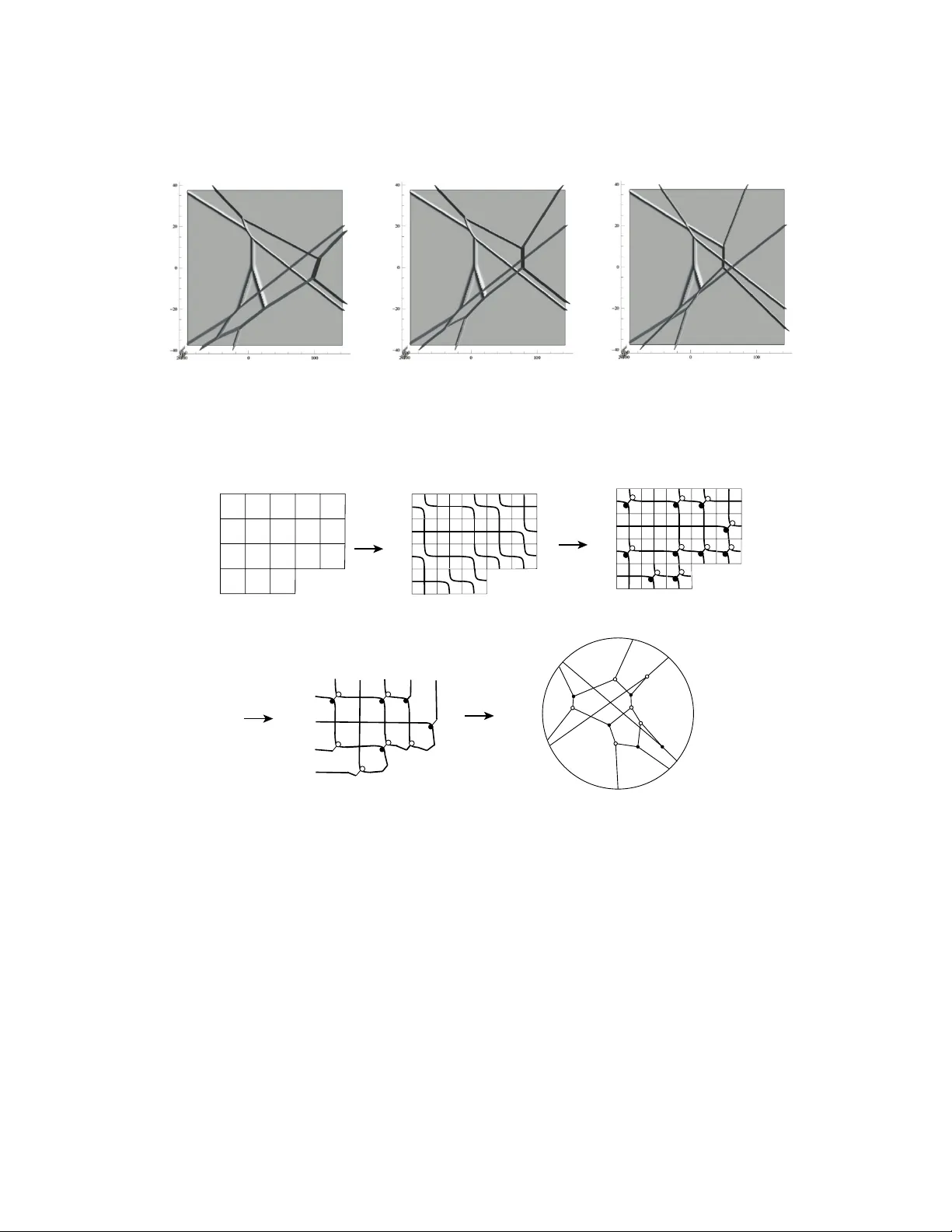
KP SOLITONS AND TOT AL POSITIVITY F OR THE GRASSMANNIAN YUJI KOD AMA AND LA UREN WILLIAMS Abstract. Soliton solutions of the KP equation hav e been studied since 1970, when Kadomtsev and Petviash vili proposed a tw o-dimensional nonlinear dispersive wa v e equation no w known as the KP equation. It is well-kno wn that one can use the W ronskian metho d to construct a soliton solution to the KP equation from each p oin t of the real Grassmannian Gr k,n . More recently , several authors [3, 15, 2, 4, 6] hav e studied the r e gular solutions that one obtains in this wa y: these come from points of the totally non-negative part of the Grassmannian ( Gr k,n ) ≥ 0 . In this pap er w e exhibit a surprising connection b et w een the theory of total p ositivit y for the Grassmannian, and the structure of regular soliton solutions to the KP equation. By exploiting this connection, we obtain new insights into the structure of KP solitons, as well as new interpretations of the combinatorial ob jects indexing cells of ( Gr k,n ) ≥ 0 [25]. In particular, we completely classify the spatial patterns of the soliton solutions coming from ( Gr k,n ) ≥ 0 when the absolute v alue of the time parameter is suﬃciently large. W e demonstrate an intriguing connection b et ween soliton graphs for ( Gr k,n ) > 0 and the cluster algebr as of F omin and Zelevinsky [9], and we use this connection to solve the inverse problem for generic KP solitons coming from ( Gr k,n ) > 0 . Finally we construct all the soliton graphs for ( Gr 2 ,n ) > 0 using the triangulations of an n -gon. Contents 1. In tro duction 1 2. T otal p ositivity for the Grassmannian 4 3. Soliton solutions to the KP equation 6 4. F rom soliton solutions to soliton graphs 8 5. P ermutations and soliton asymptotics 12 6. Grassmann necklaces and soliton asymptotics 14 7. Soliton graphs are generalized plabic graphs 16 8. A construction for asymptotic contour plots 18 9. X-crossings and v anishing Pl ¨ uc ker coordinates 27 10. TP Sch ub ert cells, reduced plabic graphs, and cluster algebras 31 11. The inv erse problem for soliton graphs 37 12. T riangulations of n -gon and soliton graphs for ( Gr 2 ,n ) > 0 41 References 45 1. Introduction The KP equation is a t w o-dimensional nonlinear dispersive wa ve equation given b y (1.1) ∂ ∂ x  − 4 ∂ u ∂ t + 6 u ∂ u ∂ x + ∂ 3 u ∂ x 3  + 3 ∂ 2 u ∂ y 2 = 0 , Date : Octob er 30, 2018. The ﬁrst author was partially supp orted by NSF gran ts DMS-0806219 and DMS-1108813. The second author was partially supported by the NSF grant DMS-0854432 and an Alfred Sloan F ellowship. 1 2 YUJI KOD AMA AND LAUREN WILLIAMS where u = u ( x, y , t ) represents the wa v e amplitude at the p oint ( x, y ) in the xy -plane for ﬁxed time t . The equation was proposed b y Kadomtsev and P eviash vili in 1970 to study the transversal stabilit y of the soliton solutions of the Korteweg-de V ries (KdV) equation [13]. The KP equation can also b e used to describ e shallow water wa ves, and in particular, the equation pro vides an excellen t model for the resonan t interaction of those wa v es (see [16] for recen t progress). The equation has a rich mathematical structure, and is no w considered to be the prototype of an in tegrable nonlinear disp ersiv e w a v e equation with tw o spatial dimensions (see for example [23, 1, 7, 22, 12]). One of the main breakthroughs in the KP theory w as given by Sato [27], who realized that solutions of the KP equation could b e written in terms of p oin ts on an inﬁnite-dimensional Grassmannian. The presen t pap er deals with a real, ﬁnite-dimensional v ersion of the Sato theory; in particular, we are in terested in solutions that are regular in the en tire xy -plane, where they are lo calized along certain ra ys. W e call suc h solution line-soliton solution , and they can b e constructed from a p oin t A of the real Grassmannian [27, 28, 10, 12]. In this pap er, we denote by u A ( x, y , t ) the solution asso ciated to A . Recen tly several authors hav e work ed on classifying the regular line-soliton solutions [3, 15, 2, 4, 6]. These solutions come from p oin ts of the total ly non-ne gative p art of the Gr assmannian , that is, those p oin ts of the real Grassmannian whose Pl ¨ uck er co ordinates are all non-negativ e. They found a large v ariety of soliton solutions which were previously o v erlooked b y those using the Hirota method of a p erturbation expansion [12]. In the generic situation, the asymptotic pattern at y → ±∞ of the solution consists of n line-solitons. Ho wev er, b ecause of the nonlinearity in the KP equation, the interaction pattern of the soliton solutions are very com plex. Figure 1 illustrates the time evolution of the pattern of a line-soliton solution. Eac h ﬁgure shows the contour plot of the solution at a ﬁxed time t in the xy -plane with x in the horizontal and y in the vertical directions. One of the main goals of this pap er 100 200 -100 -200 0 100 200 -100 -200 0 -200 -100 100 200 0 -200 -100 100 200 0 t = 70 t = 0 100 200 -100 -200 0 -200 -100 100 200 0 t = -70 Figure 1. Time evolution of the spatial pattern of a soliton solution. The ﬁgures illustrate the contour plots of the solution (see Example 8.16 to reconstruct the ﬁgures). is to give a combinatorial classiﬁcation of the patterns generated by the line-soliton solutions as in the ﬁgures. Recen tly Postnik o v [25] studied the totally non-negativ e part of the Grassmannian ( Gr k,n ) ≥ 0 from a combinatorial p oin t of view. T otal positivity has attracted a lot of interest in the last tw o decades, largely due to w ork of Lusztig [19, 20], who introduced the totally p ositiv e and non-negativ e parts of real reductiv e groups and ﬂag v arieties (of whic h the Grassmannian is an important example). Postnik ov ga ve a decomp osition of ( Gr k,n ) ≥ 0 in to p ositr oid c el ls , b y sp ecifying whic h Pl ¨ uc k er co ordinates are strictly p ositiv e and which are zero. He also introduced several remark able families of com binatorial ob jects, including de c or ate d p ermutations, Γ -diagr ams, plabic gr aphs, and Gr assmann ne cklac es, in order to index the cells and describe their prop erties. KP SOLITONS AND TOT AL POSITIVITY FOR THE GRASSMANNIAN 3 W e are interested in the wa ve pattern generated by a soliton solution u A ( x, y , t ) in the xy -plane for ﬁxed time t . W e then consider a c ontour plot C ( u A , t ) for eac h t in the xy -plane whic h is a tr opic al curve appro ximating the p ositions in the plane where the corresp onding w a ve has a peak, see Figure 1. While the lo cal interactions of arbitrary contour plots are extremely complicated, it is possible to understand their asymptotic structure for | y |  0. Moreov er, if we take the limit as the time v ariable t go es to inﬁnit y (or more generally , some of the symmetry parameters of the KP equation, denoted b y t = ( t 3 , t 4 , t 5 , . . . ) with t 3 = t , also go to inﬁnity), and rescale x and y accordingly , we obtain an asymptotic c ontour plot , whose com binatorial structure is muc h more tractable. W e then asso ciate to eac h asymptotic con tour plot a soliton gr aph by forgetting the metric structure of the pattern but remem b ering the top ological structure. In this pap er w e establish a tight connection b et w een total p ositivit y on the Grassmannian and the regular soliton solutions of the KP equation. This allows us to apply mac hinery from total positivity to understand soliton solutions of the KP equation. In particular: • w e classify the soliton graphs and asymptotic contour plots coming from ( Gr k,n ) ≥ 0 when t → ±∞ (Theorems 8.5 and 8.9); • w e demonstrate an intriguing connection b etw een soliton graphs for ( Gr k,n ) > 0 and the cluster algebr as of F omin and Zelevinsky [9] (Theorem 10.12); • w e solv e the inverse pr oblem for KP solitons coming from ( Gr k,n ) > 0 , and from ( Gr k,n ) ≥ 0 when | t |  0 (Theorems 11.4 and 11.2). • w e classify all soliton graphs and asymptotic con tour plots coming from ( Gr 2 ,n ) > 0 , and sho w that these soliton graphs are in bijection with triangulations of a p olygon (Theorem 12.2). Note that prior to our work almost nothing was kno wn ab out the classiﬁcation of soliton graphs, except in the cases of ( Gr 1 ,n ) > 0 [8], and ( Gr 2 , 4 ) ≥ 0 [6]. In the other direction, w e giv e a KP soliton interpretation to nearly all of Postnik o v’s com binatorial ob jects, as well as a new characterization of r e duc e d plabic gr aphs (Theorem 10.5). The structure of the pap er is as follo ws. In Sections 2 and 3 we provide background on total p ositivit y on the Grassmannian, and soliton solutions to the KP equation. In Section 4 we explain ho w to asso ciate soliton graphs to soliton solutions of the KP equation. In the next four sections (Sections 5, 6, 7, and 8) we explain the relationships b etw een combinatorial ob jects lab eling p ositroid cells and the corresp onding soliton solutions. In particular, we explain how (decorated) p erm utations and Grassmann nec klaces con trol the asympototics of soliton graphs when | y |  0, and how Γ -diagrams con trol the soliton graphs at | t |  0. W e also explain the connection b et w een plabic graphs and soliton graphs. In Section 9 we explain how the existence of X -crossings in contour plots corresp onds to “t wo- term” Pl¨ uc ker relations. In Section 10 w e pro v e that generically , the dominan t exponentials labeling the regions of a soliton graph for ( Gr k,n ) > 0 comprise a cluster for the cluster algebr a of Gr k,n . In Section 11 w e address the in v erse problem for regular soliton solutions to the KP equation. Finally , in Section 12, w e completely classify the soliton graphs coming from solutions u A for A ∈ ( Gr 2 ,n ) > 0 , and c onstruct them all using triangulations of an n -gon. The present paper pro vides proofs of the results announced in [17]. In the sequel to this work [18] we ha ve extended man y of the results of the presen t paper from the non-negative part of the Grassmannian to the real Grassmannian. In a future pap er we plan to mak e a detailed study of the relationship b et ween cluster tr ansformations and the ev olution of soliton graphs. A cknowledgements: The authors are grateful for the hospitality of the math departments at UC Berk eley and Ohio State, where some of this w ork was carried out. They are also grateful to Sara Billey , and to an anonymous referee, whose comments helped them to greatly improv e the exp osition. 4 YUJI KOD AMA AND LAUREN WILLIAMS 2. Tot al positivity for the Grassmannian In this section w e review the Grassmannian Gr k,n and Postnik ov’s decomp osition of its non-negativ e part ( Gr k,n ) ≥ 0 in to p ositroid cells [25]. Note that our conv entions sligh tly diﬀer from those of [25]. The real Grassmannian Gr k,n is the space of all k -dimensional subspaces of R n . An elemen t of Gr k,n can b e view ed as a full-rank k × n matrix mo dulo left multiplication by nonsingular k × k matrices. In other words, tw o k × n matrices represen t the same p oint in Gr k,n if and only if they can b e obtained from each other by row op erations. Let  [ n ] k  b e the set of all k -element subsets of [ n ] := { 1 , . . . , n } . F or I ∈  [ n ] k  , let ∆ I ( A ) denote the maximal minor of a k × n matrix A lo cated in the column set I . The map A 7→ (∆ I ( A )), where I ranges ov er  [ n ] k  , induces the Pl¨ ucker emb e dding Gr k,n  → RP ( n k ) − 1 . F or M ⊆  [ n ] k  , the matr oid str atum S M is the set of elements of Gr k,n represen ted b y all k × n matrices A with ∆ I ( A ) 6 = 0 for I ∈ M and ∆ J ( A ) = 0 for J / ∈ M . The decomp osition of Gr k,n in to the strata S M is called the the matr oid str atiﬁc ation . Deﬁnition 2.1 . The total ly non-ne gative Gr assmannian ( Gr k,n ) ≥ 0 (resp ectiv ely , total ly p ositive Gr ass- mannian ( Gr k,n ) > 0 ) is the subset of Gr k,n that can b e represented by k × n matrices A with all ∆ I ( A ) non-negativ e (resp ectiv ely , p ositiv e). P ostniko v [25] studied the decomp osition of ( Gr k,n ) ≥ 0 induced by the matroid stratiﬁcation. More sp eciﬁcally , for M ⊆  [ n ] k  , he deﬁned the p ositr oid c el l S tnn M as the set of elements of ( Gr k,n ) ≥ 0 represen ted by all k × n matrices A with ∆ I ( A ) > 0 for I ∈ M and ∆ J ( A ) = 0 for J 6∈ M . It turns out that each nonempt y S tnn M is actually a cell [25], and that this decomposition of ( Gr k,n ) ≥ 0 is a CW complex [26]. Note that ( Gr k,n ) > 0 is a p ositroid cell; it is the unique p ositroid cell in ( Gr k,n ) ≥ 0 of top dimension k ( n − k ). Postnik o v show ed that the cells of ( Gr k,n ) ≥ 0 are naturally lab eled by (and in bijection with) the following com binatorial ob jects [25]: • Grassmann necklaces I of type ( k , n ) • decorated p erm utations π : on n letters with k w eak excedances • equiv alence classes of r e duc e d plabic gr aphs of type ( k , n ) • Γ -diagrams of type ( k , n ). F or the purp ose of studying solitons, we are in terested only in the irr e ducible p ositroid cells. Deﬁnition 2.2 . W e sa y that a p ositroid cell S tnn M is irr e ducible if the reduced-row echelon matrix A of an y p oin t in the cell has the following properties: • Eac h column of A contains at least one nonzero element. • Eac h row of A contains at least one nonzero element in addition to the pivot. The irreducible p ositroid cells are indexed by: • irreducible Grassmann necklaces I of type ( k , n ) • derangemen ts π on n letters with k excedances • equiv alence classes of irr e ducible r e duc e d plabic gr aphs of type ( k , n ) • irreducible Γ -diagrams of type ( k , n ). W e now review the deﬁnitions of these ob jects and some bijections among them. Deﬁnition 2.3 . An irr e ducible Gr assmann ne cklac e of typ e ( k , n ) is a sequence I = ( I 1 , . . . , I n ) of subsets I r of [ n ] of size k such that, for i ∈ [ n ], I i +1 = ( I i \ { i } ) ∪ { j } for some j 6 = i . (Here indices i are taken mo dulo n .) Example 2.4 . I = (1257 , 2357 , 3457 , 4567 , 5678 , 6789 , 1789 , 1289 , 1259) is an example of a Grassmann nec klace of t yp e (4 , 9). KP SOLITONS AND TOT AL POSITIVITY FOR THE GRASSMANNIAN 5 Deﬁnition 2.5 . A der angement π = ( π (1) , . . . , π ( n )) is a p ermutation π ∈ S n whic h has no ﬁxed p oints. An exc e danc e of π is a pair ( i, π ( i )) such that π ( i ) > i . W e call i the exc e danc e p osition and π ( i ) the exc e danc e value . Similarly , a nonexc e danc e is a pair ( i, π ( i )) such that π ( i ) < i . R emark 2.6 . A de c or ate d p ermutation is a permutation in whic h ﬁxed points are colored with one of t wo colors. Under the bijection b et w een positroid cells and decorated p ermutations, the irreducible p ositroid cells corresp ond to derangements, i.e. those decorated p erm utations which ha v e no ﬁxed p oin ts. Example 2.7 . The derangement π = (6 , 7 , 1 , 2 , 8 , 3 , 9 , 4 , 5) ∈ S 9 has excedances in p ositions 1 , 2 , 5 , 7. Deﬁnition 2.8 . A plabic gr aph is a planar undirected graph G dra wn inside a disk with n b oundary vertic es 1 , . . . , n placed in counterclockwise order around the b oundary of the disk, suc h that each b oundary vertex i is inciden t to a single edge. 1 Eac h in te rnal vertex is colored blac k or white. See Figure 2 for an example. 1 2 3 4 5 + + + + + + + + + + + + + + + + + + + + 0 0 0 0 0 0 0 0 0 0 0 0 0 0 0 0 0 0 0 0 0 0 0 k n - k λ = (10, 9, 9, 8, 5, 2) k = 6, n = 16 Figure 2. A plabic graph, and an irreducible Le-diagram L = ( λ, D ) k,n . Deﬁnition 2.9 . Fix k and n . Let Y λ denote the Y oung diagram of the partition λ . A Γ -diagr am (or Le-diagram) L = ( λ, D ) k,n of type ( k , n ) is a Y oung diagram Y λ con tained in a k × ( n − k ) rectangle together with a ﬁlling D : Y λ → { 0 , + } which has the Γ -pr op erty : there is no 0 which has a + ab o v e it in the same column and a + to its left in the same row. A Γ -diagram is irr e ducible if each ro w and eac h column contains at least one +. See the righ t of Figure 2 for an example of an irreducible Γ -diagram. The or em 2.10 . [25, Theorem 17.2] Let S tnn M b e a positroid cell in ( Gr k,n ) ≥ 0 . F or 1 ≤ r ≤ n , let I r b e the element of M which is lexicographically minimal with resp ect to the order r < r + 1 < · · · < n < 1 < 2 < . . . r − 1. Then I ( M ) := ( I 1 , . . . , I n ) is a Grassmann necklace of type ( k , n ). L emma 2.11 . [25, Lemma 16.2] Giv en an irreducible Grassmann nec klace I , deﬁne a derangemen t π = π ( I ) b y requiring that: if I i +1 = ( I i \ { i } ) ∪ { j } for j 6 = i , then π ( j ) = i . 2 Indices are tak en mo dulo n . Then I → π ( I ) is a bijection from irreducible Grassmann necklaces I = ( I 1 , . . . , I n ) of type ( k , n ) to derangements π ( I ) ∈ S n with k excedances. The excedances of π ( I ) are in p ositions I 1 . Example 2.12 . If I and π are deﬁned as in Examples 2.4 and 2.7, then π ( I ) = π . Deﬁnition 2.13 . Giv en a Γ -diagram L contained in a k × ( n − k ) rectangle, label its southeast border with the num b ers 1 , 2 , . . . , n , starting at the northeast corner. Replace eac h + with an “elb o w” and eac h 0 with a “cross”; see Figure 3. Now trav el along eac h “pip e” from southeast to north w est, and lab el the end of a pip e with the same num b er that lab eled its origin. Finally , we deﬁne a p erm utation π = π ( L ) as follows. If i is the lab el of a vertical edge on the southeast b order of L , then set π ( i ) equal to the lab el of the vertical edge on the other side of that ro w. If i is the label of a horizontal edge on the southeast b order of L , then set π ( i ) equal to the label of the horizontal edge on the opp osite side of that column. See Figure 3. 6 YUJI KOD AMA AND LAUREN WILLIAMS + + + + 0 0 0 1 2 3 4 5 6 7 98 1 2 3 8 9 4 5 6 7 0 + + + + + + 0 0 Figure 3. The Le-diagram L together with the computation of π ( L ) = (7 , 4 , 2 , 9 , 1 , 3 , 8 , 6 , 5). Pr op osition 2.14 . The map deﬁned ab ov e gives a bijection from irreducible Γ -diagrams contained in a k × ( n − k ) rectangle to derangemen ts on n letters with k excedances. Pr o of . This map can b e shown to coincide with that from [30, Section 2], and up to a conv en tion c hange, coincides with the map in [25, Corollary 20.1]. R emark 2.15 . Consider a p ositroid cell S tnn M , and supp ose that the Grassmann nec klace I , the derange- men t π , and the Γ -diagram L , satisfy I = I ( M ), and π = π ( I ) = π ( L ). Then we also refer to this cell as S tnn M ( I ) , S tnn M ( L ) , S tnn I , S tnn π , S tnn L , etc. 3. Soliton solutions to the KP equa tion In this section we explain how to construct a τ -function τ A ( x, y , t ) from a p oin t of Gr k,n , and then ho w to obtain a soliton solution to the KP equation from that τ -function. 3.1. F rom a p oint of the Grassmannian to a τ -function. W e ﬁrst give a realization of Gr k,n with a speciﬁc basis of R n . The purpose of making this non-standard c hoice of basis is to iden tify the Pl¨ uck er em b edding of a p oint A of the Grassmannian with a particular τ -function, in (3.5) b elo w. Cho ose real parameters κ i suc h that κ 1 < κ 2 · · · < κ n . In this pap er w e will assume that the κ i ’s are generic , meaning that: • the sums p P j =1 κ i j are all distinct for any p with 1 < p < n . W e deﬁne a set of vectors { E 0 j : j = 1 , . . . , n } b y (3.1) E 0 j :=      1 κ j . . . κ n j      ∈ R n . Since all κ j ’s are distinct, the set { E 0 j : j = 1 , . . . , n } forms a basis of R n . No w deﬁne an n × n matrix E 0 = ( E 0 1 , . . . , E 0 n ) which is the V andermonde matrix in the κ j ’s, and let A b e a full-rank k × n matrix represen ting a point of Gr k,n . Then the v ectors { F 0 i ∈ R n : i = 1 , . . . , k } span a k -dimensional subspace in R n , where F 0 i is deﬁned by F 0 i := n P j =1 a i,j E 0 j , or ( F 0 1 , . . . , F 0 k ) = E 0 A T , 1 The conv ention of [25] w as to place the b oundary vertices in clockwise order. 2 Postnik ov’s con ven tion was to set π ( i ) = j abov e, so the permutation we are asso ciating is the inv erse one to his. KP SOLITONS AND TOT AL POSITIVITY FOR THE GRASSMANNIAN 7 where A T is the transp ose of A . F or I = { i 1 , . . . , i k } , deﬁne the v ector E 0 I = E 0 i 1 ∧ · · · ∧ E 0 i k . Then w e ha ve a realization of the Pl ¨ uc k er embedding: F 0 1 ∧ · · · ∧ F 0 k = P I ∈ ( [ n ] k ) ∆ I ( A ) E 0 I . In [27], Sato show ed that each solution of the KP equation is given by a GL ∞ -orbit on the universal Grassmannian. T o construct suc h an orbit for a ﬁnite dimensional Grassmannian, w e ﬁrst deﬁne multi- time v ariables ˆ t := ( t 1 , . . . , t m ) for m ≥ 3 which give a parameterization of the orbit. Then w e consider a deformation E ˆ t j of the vector E 0 j for j = 1 , . . . , n , given b y E ˆ t j := E 0 j exp θ j ( ˆ t ) with θ j ( ˆ t ) := m P i =1 κ i j t i . F or the KP equation, w e identify t 1 = x, t 2 = y and t 3 = t , and denote those ﬂow parameters by ˆ t = ( x, y , t ) , with t := ( t 3 , . . . , t m ) . W e now deﬁne an orbit generated by the matrix E ˆ t = ( E ˆ t 1 , . . . , E ˆ t n ) on elements of GL n , g ˆ t := E ˆ t g for each g ∈ GL n . Here w e iden tify the n × k matrix consisting of the ﬁrst k columns of g with the matrix A T , the transpose of the matrix A parametrizing a p oin t Gr k,n . Then the Pl ¨ uc k er embedding gives g · e 1 ∧ · · · ∧ e k = P 1 ≤ i 1 < ··· 0 for all ( x, y , t ) ∈ R m . Note that the τ -function deﬁned in (3.5) can b e also written in the W ronskian form (3.6) τ A ( x, y , t ) = W r( f 1 , f 2 , . . . , f k ) , 8 YUJI KOD AMA AND LAUREN WILLIAMS with the scalar functions { f j : j = 1 , . . . , k } given by ( f 1 , f 2 , . . . , f k ) T = A · ( E 1 , E 2 , . . . , E n ) T , where E j is the exp onential function deﬁned by E j := exp θ j ( x, y , t ). 3.2. F rom the τ -function to solutions of the KP equation. It is well known (see [12, 4, 5, 6]) that if we set x = t 1 , y = t 2 , t = t 3 (treating the other t i ’s as constants), the τ -function deﬁned in (3.6) giv es rise to a soliton solution of the KP equation (1.1), namely (3.7) u A ( x, y , t ) = 2 ∂ 2 ∂ x 2 ln τ A ( x, y , t ) . The other t j ’s corresp ond to the ﬂo w parameters of the higher symmetries of the KP equation, and the set of the symmetries is called the KP hier ar chy (see e.g. [22]). It is easy to show that if A ∈ ( Gr k,n ) ≥ 0 , then suc h a solution u A ( x, y , t ) is regular for all t j ∈ R . In the sequel to this paper [18], w e show that if u A ( x, y , t ) is regular for all x, y and t = t 3 (with the other t i ’s ﬁxed constants), then A ∈ ( Gr k,n ) ≥ 0 . (In [16, Prop osition 4.1], a w eaker statemen t w as pro ved: if u A ( x, y , t ) is regular for all t j ∈ R , then A ∈ ( Gr k,n ) ≥ 0 .) F or this reason w e are mainly in terested in solutions u A ( x, y , t ) of the KP equation which come from p oints A of ( Gr k,n ) ≥ 0 . 4. From soliton solutions to soliton graphs In this section w e deﬁne certain tropical curves asso ciated with soliton solutions: c ontour plots and asymptotic c ontour plots . W e also deﬁne the notion of soliton gr aph . 4.1. Con tour plots. One can visualize a solution u A ( x, y , t ) in the xy -plane by drawing level sets of the solution when the co ordinates t = ( t 3 , . . . , t m ) are ﬁxed. F or each r ∈ R , we denote the corresp onding lev el set b y C r ( t ) := { ( x, y ) ∈ R 2 : u A ( x, y , t ) = r } . Figure 4 depicts b oth a three-dimensional image of a solution u A ( x, y , t ) for ﬁxed t , as well as multiple lev el sets C r . These levels sets are lines parallel to the line of the wa v e p eak. Example 4.1 . W e compute the soliton solution u A ( x, y , t ) associated to the 1 × 2 matrix A = (1 a ) with a > 0, considered as an element of ( Gr 1 , 2 ) > 0 . W rite E 1 = e θ 1 and aE 2 = e θ 2 +ln a = e ˜ θ 2 . Then the τ -function τ A and the soliton solution u A are given b y τ A ( x, y , t ) = e θ 1 + e ˜ θ 2 = 2 e 1 2 ( θ 1 + ˜ θ 2 ) cosh 1 2 ( θ 1 − ˜ θ 2 ) , and u A ( x, y , t ) = 1 2 ( κ 1 − κ 2 ) 2 sec h 2 1 2 ( θ 1 − ˜ θ 2 ) . This is a line-soliton solution , and the p eak of the solution (w a v e crest) is giv en by the equation θ 1 = ˜ θ 2 , i.e. x + ( κ 1 + κ 2 ) y + m P j =3 h j − 1 ( κ 1 , κ 2 ) t j = − 1 κ 2 − κ 1 ln a. where we ha v e used κ j +1 2 − κ j +1 1 = ( κ 2 − κ 1 ) h j ( κ 1 , κ 2 ) with h j ( κ 1 , κ 2 ) = P p + q = j κ p 1 κ q 2 . F or each ﬁxed t , θ 1 = ˜ θ 2 giv es a line whic h divides the xy -plane in to t w o regions. The exp onen tial E 1 dominates in the region including x  0, and E 2 dominates the other region where x  0. W e label eac h region by its dominant exp onen tial. Figure 4 depicts u A ( x, y , t ), where t = (0 , . . . , 0), a = 1, and ( κ 1 , κ 2 ) = ( − 1 , 2). KP SOLITONS AND TOT AL POSITIVITY FOR THE GRASSMANNIAN 9 Figure 4. A line-soliton solution u A ( x, y , t ) where A = (1 , 1) ∈ ( Gr 1 , 2 ) ≥ 0 , depicted via the 3-dimensional proﬁle u A ( x, y , 0 ), and the lev el sets of u A ( x, y , 0). E i represen ts the dominant exponential in each region. T o study the b eha vior of u A ( x, y , t ) for A ∈ S M , we consider the dominant exp onen tials at each p oin t ( x, y , t ), and we deﬁne ˆ f A ( x, y , t ) = max J ∈M { ∆ J ( A ) E J ( x, y , t ) } = max J ∈M { ∆ J ( A ) K J E j 1 . . . E j k } = max J ∈M  exp  ln  ∆ J ( A ) K J  + Θ J ( x, y , t )  , where K J and Θ J ( x, y , t ) are deﬁned in (3.3) and (3.4). F rom (3.5), we see that τ A can be appro ximated b y ˆ f A . Let f A ( x, y , t ) b e the closely related function (4.1) f A ( x, y , t ) = max J ∈M  ln  ∆ J ( A ) K J  + Θ J ( x, y , t )  . Note that at a giv en p oin t ( x, y , t ), f A ( x, y , t ) is equal to a given term if and only if ˆ f A ( x, y , t ) is equal to the exp onentiated v ersion of that term. Deﬁnition 4.2 . Given a solution u A ( x, y , t ) of the KP equation as in (3.7), we deﬁne C ( u A , t 0 ) for ﬁxed t = t 0 to b e the lo cus in R 2 where f A ( x, y , t = t 0 ) is not linear, and we refer to this as a c ontour plot of the solution u A ( x, y , t ). 4.2. Asymptotic con tour plots. Some of this paper will b e concerned with the contour plots for large scales of the v ariables ( x, y , t 3 , . . . , t m ). In this case, each of the constant terms ln  ∆ J ( A ) K J  in f A ( x, y , t ) is negligible. More precisely , we use rescaled v ariables ¯ t := ( ¯ x, ¯ y , a ) deﬁned by ˆ t = ( x, y , t ) = s ( ¯ x, ¯ y , a ) , for some s  0 . W e then approximate f A b y the function f M ( ¯ x, ¯ y , a ) := max J ∈M { Θ J ( ¯ x, ¯ y , a )) } , whic h is obtained by taking the limit of 1 s f A ( x, y , t ) as s → ∞ . Deﬁnition 4.3 . W e deﬁne the asymptotic c ontour plot C a 0 ( M ) for ﬁxed a = a 0 to b e the lo cus in R 2 where f M ( ¯ x, ¯ y , a = a 0 ) is not linear. Most of this pap er will be concerned with the asymptotic con tour plots C a 0 ( M ) for a 0 = ± (1 , 0 , 0 , . . . ), which we denote by C ± ( M ). These asymptotic contour plots are the limits of the ﬁnite con tour plots C ( u A , t 0 ) for A ∈ S M and ˆ t = s ¯ t in the limit s → ∞ . 10 YUJI KOD AMA AND LAUREN WILLIAMS Note that eac h region of the complemen t of C ( u A , t 0 ) is a domain of linearit y for f A ( x, y , t 0 ), and hence each region is naturally asso ciated to a dominant exp onential ∆ J ( A ) E J ( x, y , t 0 ) from the τ - function (3.5). W e label this region b y E J or Θ J . W e label regions of the complement of eac h asymptotic con tour plot in the same w ay . A line-soliton is a ﬁnite or unbounded line segmen t in a contour plot (or asymptotic contour plot) whic h represents a balance b et ween t w o dominant exp onentials in the τ -function. Lemma 4.4 and (4.2) pro vide the equation for a line-soliton. Eac h contour plot C ( u A , t 0 ) and each asymptotic contour plot C a 0 ( M ) consists of line segments, some of which ha ve ﬁnite length, while others are unbounded and extend in the y direction to ±∞ . The un b ounded lines are all line-solitons, which we call unb ounde d line-solitons. The ﬁnite line segments in asymptotic contour plots are all line-solitons, but some of the ﬁnite line segments in non-asymptotic con tour plots may represen t phase shifts , which ha ve lengths whic h are determined by the κ -parameters (see [6, page 35] for details). L emma 4.4 . [6, Proposition 5] Consider a line-soliton in a contour plot. The index sets of the dominan t exp onen tials of the τ -function in adjacent regions of the con tour plot in the xy -plane are of the form { i, m 2 , . . . , m k } and { j, m 2 , . . . , m k } . According to Lemma 4.4, those tw o exp onential terms hav e k − 1 common phases, so w e call the line separating them a line-soliton of typ e [ i, j ], or simply an [ i, j ] -soliton . Lo cally we hav e τ A ≈ ∆ I ( A ) E I + ∆ J ( A ) E J = (∆ I ( A ) K I E i + ∆ J ( A ) K J E j ) k Y l =2 E m l =  e θ i +ln(∆ I ( A ) K I ) + e θ j +ln(∆ J ( A ) K J  k Y l =2 E m l , so the equation for this line-soliton is (4.2) x + ( κ i + κ j ) y + m P p =3 h p − 1 ( κ i , κ j ) t p = − 1 κ j − κ i ln ∆ J ( A ) K J ∆ I ( A ) K I . See also Example 4.1. The equation for a line-soliton in an asymptotic con tour plot is the same as in (4.2), except that the constan t term on the righ t-hand side is 0 (this is immediate from the deﬁnition of asymptotic contour plot). R emark 4.5 . Consider a line-soliton given by (4.2) for ﬁxed t = ( t 3 , . . . , t m ). Compute the angle Ψ [ i,j ] b et w een the line-soliton of type [ i, j ] and the positive y -axis, measured in the counterclockwise direction, so that the negativ e x -axis has an angle of π 2 and the positive x -axis has an angle of − π 2 . Then tan Ψ [ i,j ] = κ i + κ j , so we refer to κ i + κ j as the slop e of the [ i, j ] line-soliton (see Figure 4). Also note that the lo cation of the line dep ends on the ratio of the Pl ¨ uc k er co ordinates corresp onding to the dominan t exp onen tials on either side of the line-soliton. W e will b e interested in the combinatorial structure of asymptotic contour plots, that is, the pattern of ho w line-solitons in teract with eac h oth er. Generically w e expect a point at whic h sev eral line-solitons meet to hav e degree 3; we regard such a point as a triv alent vertex. Three line-solitons meeting at a triv alent v ertex exhibit a r esonant inter action (this corresp onds to the b alancing c ondition for a tropical curv e), see Section 4.4. One may also ha ve t w o line-solitons whic h cross o v er eac h other, forming an X -shap e: we call this an X -cr ossing , but do not regard it as a vertex. See Figure 5 for examples. W e will give more details ab out X-crossings in Section 9. KP SOLITONS AND TOT AL POSITIVITY FOR THE GRASSMANNIAN 11 Deﬁnition 4.6 . A contour plot C ( u A , t ) is called generic if there exists an  > 0 suc h that C ( u A , t 0 ) has the same top ology as C ( u A , t ) for any t 0 satisfying k t − t 0 k <  . Similarly , an asymptotic contour plot C a ( M ) is called generic if there exists an  > 0 suc h that C a 0 ( M ) has the same top ology as C a ( M ) for an y a 0 satisfying k a − a 0 k <  . Here the norm k · k is the usual Euclidian norm in R m − 2 . 4.3. Soliton graphs. The following notion of soliton gr aph forgets the metric data of the asymptotic con tour plot, but preserves the data of how line-solitons interact and which exponentials dominate. Deﬁnition 4.7 . Let C a 0 ( M ) b e an asymptotic con tour plot with n unbounded line-solitons. Color a triv alent vertex blac k (resp ectively , white) if it has a unique edge extending do wnw ards (respec tiv ely , up wards) from it. Lab el a region b y E I if the dominant exp onen tial in that region is ∆ I E I . Lab el eac h edge (line-soliton) by the typ e [ i, j ] of that line-soliton. Preserve the top ology of the metric graph, but forget the metric structure. Em bed the resulting graph with bicolored vertices into a disk with n b oundary vertices, replacing each unbounded line-soliton with an edge that ends at a b oundary vertex. W e call this lab eled graph the soliton gr aph G a 0 ( M ). Abusing notation, w e will often refer to the edges of G a 0 ( M ) as line-solitons , and use the terminology unb ounde d line-solitons and unb ounde d r e gions to refer to the edges and regions inciden t to the b oundary of the disk. [4,9] [2,4] [1,7] [5,9] [6,8] [3,6] [1,5] [2,3] [2,5] [4,5] [4,8] [1,9] [1,3] [1,6] E 1247 E 4789 [7,9] [7,8] [4,6] [4,9] [2,4] [1,7] [5,9] [6,8] [3,6] [1,5] [2,3] [7,8] E 1247 E 4789 Figure 5. Example of an asymptotic contour plot and the soliton graph asso ciated to S tnn π with π = (7 , 4 , 2 , 9 , 1 , 3 , 8 , 6 , 5). See Figure 5 for an example of a soliton graph. Although we ha ve not lab eled all regions or all edges, the remaining lab els can b e determined using Lemma 4.4. 4.4. Resonance of line-solitons. In this section we explain the physical meaning of triv alen t vertices in the contour plot. It follows from Example 4.1 that a line-soliton of [ i, j ]-type has the form u = 1 2 ( κ i − κ j ) 2 sec h 2 1 2 Θ [ i,j ] ( x, y , t ) , where the phase function Θ [ i,j ] ( x, y , t ) is given b y Θ [ i,j ] ( x, y , t ) = ( κ j − κ i ) x + ( κ 2 j − κ 2 i ) y + m P s =3 Ω ( s ) [ i,j ] ( κ ) t s + Θ 0 [ i,j ] ( κ, A ) , with Ω ( s ) [ i,j ] ( κ ) := κ s j − κ s i , and Θ 0 [ i,j ] ( κ, A ) := ln ∆ J ( A ) K J ∆ I ( A ) K I . 12 YUJI KOD AMA AND LAUREN WILLIAMS In particular, the co eﬃcients of x, y and t = t 3 are called the wa ven um ber-vector and the frequency , and they are given b y (4.3) K [ i,j ] := ( K x [ i,j ] , K y [ i,j ] ) = ( κ j − κ i , κ 2 j − κ 2 i ) , Ω [ i,j ] = κ 3 j − κ 3 i . There is an algebraic relation, called the disp ersion r elation of the KP equation, among K [ i,j ] and Ω [ i,j ] , which is given b y (4.4) D ( K [ i,j ] , Ω [ i,j ] ) := − 4Ω [ i,j ] K x [ i,j ] + ( K x [ i,j ] ) 4 + 3( K y [ i,j ] ) 2 = 0 . See [32, Chapter 11.1] for more details. This implies that if a plane wa v e of the form φ ( K j · x + Ω j t ) is a solution of the KP equation, then K j and Ω j m ust satisfy the disp ersion relation. Note that the w av enum b er-vectors and the frequency giv en in (4.3) satisfy (4.4), i.e. D ( K j , Ω j ) = 0. In wa ve theory , if for tw o plane wa v es φ i ( K i · x + Ω i t ) for i = 1 and 2 we hav e D ( K 1 + K 2 , Ω 1 + Ω 2 ) = 0 , then as a result, a third wa v e can b e generated. Moreov er, the new wa v e φ 3 ( K 3 · x + Ω 3 t ) satisﬁes the so-called r esonant c onditions , K 3 = K 1 + K 2 , and Ω 3 = Ω 1 + Ω 2 . In the KP disp ersion relation, the line-solitons of t yp es [ i, j ], [ j,  ], and [ i,  ] (here i < j <  ) trivially satisfy the resonant conditions, i.e. K [ i,` ] = K [ i,j ] + K [ j,` ] , and Ω [ i,` ] = Ω [ i,j ] + Ω [ j,` ] . (4.5) The resonant relations (4.5) also hold for the higher terms Ω ( s ) [ i,j ] for s = 4 , . . . , m , i.e. Ω ( s ) [ i,` ] = Ω ( s ) [ i,j ] + Ω ( s ) [ j,` ] for s = 4 , . . . , m. This means that resonant interactions arise quite naturally in the KP hierarc h y , and eac h 3-w a ve resonan t interaction appears as a triv alen t v ertex in the contour plot. A t that triv alen t vertex, since the slop e of each soliton is giv en by tan Ψ [ i,j ] = κ i + κ j , those three solitons app ear as [ i, j ] , [ j, l ] and [ i, l ] in coun terclockwise order. This condition led us to disco v er a new characterization of reduced plabic graphs, which we describ e in Section 10. Note also that in the contour plot, one ma y interpret equation (4.5) as the b alancing c ondition for a tropical curve. 5. Permut a tions and soliton asymptotics Giv en a contour plot C ( u A , t 0 ) where A b elongs to an irreducible positroid cell, w e show that the lab els of the un bounded solitons allow us to determine whic h p ositroid cell A belongs to. Con v ersely , giv en A in the irreducible p ositroid cell S tnn π , we can predict the asymptotic b eha vior of the un bounded solitons in C ( u A , t 0 ). The or em 5.1 . Supp ose A is an element of an irreducible p ositroid cell in ( Gr k,n ) ≥ 0 . Consider the con tour plot C ( u A , t 0 ) for an y time t 0 . Then there are k unbounded line-solitons at y  0 which are lab eled by pairs [ e r , j r ] with e r < j r , and there are n − k un b ounded line-solitons at y  0 which are lab eled by pairs [ i r , g r ] with i r < g r . W e obtain a derangement in S n with k excedances b y setting π ( e r ) = j r and π ( g r ) = i r . Moreov er, A must belong to the cell S tnn π . The ﬁrst part of this theorem follows from work of Biondini and Chakra v arty [2, Lemma 3.4 and Theorem 3.6] (see Proposition 5.2 b elow) and Chakra v art y and Kodama [4, Prop. 2.6 and 2.9], [6, Theorem 5] (see Theorem 5.3 b elow). In particular, Chakrav arty and Ko dama had already asso ciated a derangement π to A , but it w as not clear how this π was related to the derangement indexing the cell con taining A . Our contribution is a pro of that the derangemen t π is precisely the derangemen t lab eling KP SOLITONS AND TOT AL POSITIVITY FOR THE GRASSMANNIAN 13 the cell S tnn π that A b elongs to (see Prop osition 5.4) 3 . This fact is the ﬁrst step tow ards establishing that v arious other combinatorial ob jects in bijection with p ositroid cells (Grassmann necklaces, plabic graphs) carry useful information ab out the corresp onding soliton solutions. Giv en a matrix A with n columns, let A ( k, . . . ,  ) be the submatrix of A obtained from columns k , k + 1 , . . . ,  − 1 ,  , where the columns are listed in the circular order k, k + 1 , . . . , n − 1 , n, 1 , 2 , . . . , k − 1. Pr op osition 5.2 . [2, Lemma 3.4] Let A b e a k × n matrix represen ting an elemen t in an irreducible p ositroid cell in ( Gr k,n ) ≥ 0 , and consider the contour plot C ( u A , t 0 ) for an y time t 0 . Then there are n − k unbounded line-solitons at y  0 and k unbounded line-solitons at y  0: There is an unbounded line-soliton of C ( u A , t 0 ) at y  0 lab eled [ i, g ] with i < g if and only if (5.1) rank A ( i, . . . , g − 1) = rank A ( i + 1 , . . . , g ) = rank A ( i, . . . , g ) = rank A ( i + 1 , . . . , g − 1) + 1 . Moreo ev er, g is a non-pivot column of A . And there is an unbounded line-soliton of C ( u A , t 0 ) at y  0 lab eled [ e, j ] with e < j if and only if (5.2) rank A ( j, . . . , e − 1) = rank A ( j + 1 , . . . , e ) = rank A ( j, . . . , e ) = rank A ( j + 1 , . . . , e − 1) + 1 . Moreo ev er, e is a pivot column of A . The or em 5.3 . [4, Prop. 2.6 and 2.9][6, Theorem 5] Consider an irreducible p ositroid cell S tnn M in ( Gr k,n ) ≥ 0 , and let A b e a full rank matrix representing a p oin t in that cell. Use the notation of Prop osition 5.2. Deﬁne π ! := π ! ( M ) by setting π ! ( e ) := j and π ! ( g ) := ( i ) for each pivot e and non-piv ot g . Then π ! is a derangement on n letters with k w eak excedances. Pr op osition 5.4 . Consider an irreducible p ositroid cell S tnn M = S tnn π , where π = π ( I ( M )). Then π ! ( M ) = π . Pr o of . Consider a k × n matrix A represen ting an element in S tnn M . Then all maximal minors of A are non-negativ e, and the column indices of the non-zero minors are the subsets in M . Let us ﬁrst consider the derangement π = π ( I ( M )). Let I i = { i = x 1 , x 2 , . . . , x k } b e the lexicographically minimal minor in M with respect to the total order i < i + 1 < · · · < n < 1 < · · · < i − 1. Then I i +1 = ( I i \ { i } ) ∪ { j } is obtained from I i \ { i } b y considering the column indices in the order i + 1 , i + 2 , . . . , n, 1 , 2 , . . . , i and greedily c hoosing the earliest index h such that the columns of A indexed by the set { x 2 , . . . , x k } ∪ { h } are linearly indep endent. Then π ( h ) is deﬁned to b e i . No w consider the ranks of v arious submatrices of A obtained by selecting certain columns. Claim 0. rank A ( i + 1 , . . . , h − 1 , h ) = 1 + rank A ( i + 1 , . . . , h − 1). This claim follows from the wa y in which w e chose h ab o v e. Claim 1. rank A ( i, i + 1 , . . . , h ) = rank A ( i, i + 1 , . . . , h − 1). T o prov e this claim, w e consider t w o cases. Either x 1 < i h < i x k or x 1 < i x k < i h , where < i is the total order i < i + 1 < · · · < n < 1 < · · · < i − 1. In the ﬁrst case, the claim follows, b ecause h is not contained in the set I i but is contained in I i +1 . In the second case, rank A ( i, i + 1 , i + 2 , . . . , x k ) = k , and the index set { i, i + 1 , . . . , x k } is a strict subset of { i, i + 1 , . . . , h } , so rank A ( i, . . . , h ) = rank A ( i, . . . , h − 1) = k . No w let R = rank A ( i + 1 , i + 2 , . . . , h − 1). By Claim 0, rank A ( i + 1 , . . . , h ) = R + 1. Therefore we ha ve rank A ( i, . . . , h ) ≥ rank A ( i + 1 , . . . , h ) = R + 1. By Claim 1, rank A ( i, . . . , h ) = rank A ( i, . . . , h − 1), but rank A ( i, . . . , h − 1) ≤ R + 1, so rank A ( i, . . . , h ) ≤ R + 1. W e no w ha ve rank A ( i, . . . , h ) = R + 1. But also rank A ( i, . . . , h − 1) = rank A ( i, . . . , h ) = R + 1. W e ha ve just sho wn that rank A ( i, i + 1 , . . . , h − 1) = rank A ( i + 1 , . . . , h − 1 , h ) = rank A ( i, . . . , h ) = rank A ( i + 1 , . . . , h − 1) + 1. Comparing these rank conditions to either part of Proposition 5.2, and using Theorem 5.3, we see that π ! ( h ) = i . This shows that π ! and π coincide. R emark 5.5 . Prop osition 5.4 is closely related to results on cyclic rank matrices from [14]. 3 S. Chakrav arty informed us that he also prov ed an equiv alent prop osition. 14 YUJI KOD AMA AND LAUREN WILLIAMS [7,9] [5,8] [2,7] [1,6] [1,3] [2,4] [3,6] [4,8] [5,9] Interaction Region E 1257 E 1259 E 1289 E 1789 E 6789 E 2357 E 3457 E 4567 E 5678 Figure 6. Asymptotic line-solitons for π = (6 , 7 , 1 , 2 , 8 , 3 , 9 , 4 , 5). Each E ij kl sho ws the dominant exponential in this region. W e no w giv e a concrete algorithm for writing down the asymptotics of the soliton solutions of the KP equation. The or em 5.6 . Fix real generic paramete rs κ 1 < · · · < κ n . Let A b e a p oint in an irreducible p ositroid cell S tnn π in ( Gr k,n ) ≥ 0 . (So π has k excedances.) F or any t 0 , the asymptotic b eha vior of the con tour plot C ( u A , t 0 ) – its unbounded line-solitons and the dominant exp onen tials in its unbounded regions – can b e read oﬀ from π as follows. • F or y  0, there is an unbounded line-soliton which we lab el [ i, π ( i )] for each excedance π ( i ) > i . F rom left to right, list these solitons in decreasing order of the quan tity κ i + κ π ( i ) . • F or y  0, there is an unbounded line-soliton which w e lab el [ π ( j ) , j ] for each nonexcedance π ( j ) < j . F rom left to right, list these solitons in increasing order κ j + κ π ( j ) . • Lab el the un b ounded region for x  0 with the exp onen tial E i 1 ,...,i k , where i 1 , . . . , i k are the excedance p ositions of π . • Use Lemma 4.4 to lab el the remaining unbounded regions of the contour plot. Pr o of . The fact that the set of unbounded line-solitons are sp eciﬁed by the derangement π comes from [6, Theorem 5, page 125] and [6, Corollary 1, page 124]. It then follows from Remark 4.5 that for suﬃcien tly large y (resp ectively , suﬃciently small y ), these solitons are ordered from left to right b y decreasing (resp ectiv ely , increasing) order of their slop es κ i + κ j . Example 5.7 . Consider the positroid cell corresp onding to (6 , 7 , 1 , 2 , 8 , 3 , 9 , 4 , 5) ∈ S 9 . The algorithm of Theorem 5.6 giv es rise to the picture in Figure 6. Note that if one reads the dominant exponentials in coun terclo c kwise order, starting from the region at the left, then one reco v ers exactly the Grassmann nec klace from Examples 2.4 and 2.12. This corresp ondence will b e generalized in Theorem 6.2. 6. Grassmann neckla ces and soliton asymptotics One particularly nice class of p ositroid cells is the TP or total ly p ositive Schub ert c el ls . A TP Sc hubert cell is a p ositroid cell S tnn L whic h comes from a Γ -diagram L such that all boxes of L contain a +. Note that the in tersection of a usual Sch ub ert cell with ( Gr k,n ) ≥ 0 is a union of p ositroid cells, of whic h the one with greatest dimension is the TP Sch ube rt cell. When A lies in a TP Sch ubert cell S tnn π , w e can make another link b etw een the soliton solution u A ( x, y , t ) and the combinatorics of ( Gr k,n ) ≥ 0 . Namely , the dominan t exp onentials lab eling the un b ounded regions of the contour plot C ( u A , t ) form the Grassmann necklace asso ciated to S tnn π . It is easy to verify the following lemma. KP SOLITONS AND TOT AL POSITIVITY FOR THE GRASSMANNIAN 15 [ i k , π ( i k )] Interaction Region R 1 = E i 1,.., i k [ i 2 , π ( i 2 )] [ i 1 , π ( i 1 )] [ π ( j 1 ), j 1 ] [ π ( j 2 ), j 2 ] [ π ( j 3 ), j 3 ] [ π ( j n-k ), j n-k ] R 2 R 3 R n-k+1 R n Figure 7. Grassmann necklace ( R 1 , R 2 , . . . , R n ) in a con tour plot associated to the TP Sch ub ert cell S tnn π . L emma 6.1 . A p ositroid cell S tnn π = S tnn L of ( Gr k,n ) ≥ 0 is a TP Sch ubert cell if and only if the follo wing condition holds: If i 1 < i 2 < · · · < i k and j 1 < j 2 < · · · < j n − k are the p ositions of the excedances and nonexcedances, resp ectiv ely , of π , then π ( i 1 ) = n − k + 1, π ( i 2 ) = n − k + 2, . . . , π ( i k ) = n and π ( j 1 ) = 1, π ( j 2 ) = 2, . . . , π ( j n − k ) = n − k . W e hav e the following result. The or em 6.2 . Let A be an element of a TP Sc h ubert cell S tnn π , and consider the contour plot C ( u A , t 0 ) for an arbitrary time t 0 . Let the index sets of the dominant exponentials of the unbounded regions of C ( u A , t 0 ) be denoted R 1 , . . . , R n , where R 1 lab els the region at x  0, and R 2 , . . . , R n lab el the regions in the coun terclo c kwise direction from R 1 . Then ( R 1 , . . . , R n ) is a Grassmann necklace I , and π ( I ) = π . Theorem 6.2 is illustrated in Example 5.7. See also Figure 6. R emark 6.3 . Theorem 6.2 do es not hold if w e replace “TP Sc h ubert cell” b y “p ositroid cell.” F or exam- ple, the Grassmann nec klace asso ciated to the derangemen t π = (4 , 3 , 1 , 2) is (12 , 23 , 34 , 24). Ho w ever, if κ 1 = 0 , κ 2 = 1 , κ 3 = 1 . 5 , κ 4 = 1 . 75, then the corresp onding sequence of dominan t exp onentials labeling the unbounded regions of any con tour plot coming from the cell S tnn π is (12 , 23 , 34 , 13). R emark 6.4 . T o recov er a Grassmann necklace I = ( I 1 , . . . , I n ) from a derangemen t π ∈ S n (in verting the pro cedure of Lemma 2.11), we do the following: • Set I 1 = { i 1 , . . . , i k } , the p ositions of the excedances of π . • F or each r ≥ 1, set I r +1 = ( I r \ { r } ) ∪ { π − 1 ( r ) } . W e now prov e Theorem 6.2. Pr o of . Let i 1 < · · · < i k b e the p ositions of the excedances of π , and let j 1 < · · · < j n − k b e the p ositions of the nonexcedances. By Lemma 6.1, w e ha v e that π ( i 1 ) < π ( i 2 ) < · · · < π ( i k ), and π ( j 1 ) < π ( j 2 ) < · · · < π ( j n − k ). Deﬁne the partial order ≺ on pairs ( i, j ) of integers in { 1 , 2 , . . . , n } by setting ( i, j ) ≺ ( i 0 , j 0 ) if and only if κ i + κ j < κ i 0 + κ j 0 . Then the condition that κ 1 < κ 2 < · · · < κ n implies that ( i 1 , π ( i 1 )) ≺ ( i 2 , π ( i 2 )) ≺ · · · ≺ ( i k , π ( i k )) and ( j 1 , π ( j 1 )) ≺ · · · ≺ ( j n − k , π ( j n − k )). Using Theorem 5.6, the asymptotic directions of the con tour graph of the soliton solution are as in Figure 7. F rom the conditions on our p erm utation, w e must hav e π ( j 1 ) = 1 , π ( j 2 ) = 2 , . . . , π ( j n − k ) = n − k , and also π ( i 1 ) = n − k + 1 , π ( i 2 ) = n − k + 2 , . . . , π ( i k ) = n . Therefore the unbounded line-solitons of the con tour plot of the soliton solution are labeled as [ i l , n − k + l ] for l = 1 , . . . , k and [ m, j m ] for m = 1 , . . . , n − k . 16 YUJI KOD AMA AND LAUREN WILLIAMS Claim 1 . W e claim that if R 1 , . . . , R n are the index sets of the dominant exp onen tials in the un- b ounded regions as in Figure 7, then R ` con tains  . Therefore by Lemma 4.4, R ` +1 is obtained from R ` b y removing  and adding one more index not already in R ` . By Remark 6.4, Claim 1 implies ( R 1 , . . . , R n ) is the Grassmann necklace asso ciated to π , and therefore implies Theorem 6.2. W e ﬁrst pro ve Claim 1 for  ≤ n − k + 1. Clearly 1 ∈ R 1 , since 1 is alw ays the p osition of an excedance of a derangement. Supp ose b y induction that the claim is true up through  − 1. Then R ` = ((((( { i 1 , . . . , i k } ∪ { j 1 } ) \ { 1 } ) ∪ { j 2 } ) \ { 2 } ) · · · ∪ { j ` 1 } ) \ {  1 } . Supp ose that  / ∈ R ` . In steps 1 through  − 1, we ha v e only remov ed the num bers { 1 , 2 , . . . ,  − 1 } , and so  / ∈ { i 1 , . . . , i k } . And w e hav e only added the num b ers { j 1 , . . . , j ` − 1 } , and so  / ∈ { j 1 , . . . , j ` − 1 } . Since  / ∈ { i 1 , . . . , i k } , we hav e π (  ) <  , and so  ∈ { j 1 , . . . , j n − k } . Since  / ∈ { j 1 , . . . , j ` − 1 } , we hav e  ∈ { j ` , j ` +1 , . . . , j n − k } . But 1 < j 1 < j 2 < · · · < j n − k and so eac h elemen t in { j ` , j ` +1 , . . . , j n − k } is greater than  . This is a contradiction. Claim 2 . R n − k +1 = { π ( i 1 ) , . . . , π ( i k ) } . Note that since Claim 1 is true for  ≤ n − k + 1, R n − k +1 con tains an index for each excedance p osition i r suc h that π − 1 ( i r ) < i r < π ( i r ). (These are the elements of R 1 that remain in each R 2 , R 3 , . . . , R n − k +1 .) R n − k +1 also contains any nonexcedance p osition j r as long as it is not the case that j r = π − 1 ( j s ) for some s . That is, R n − k +1 con tains any j r suc h that π − 1 ( j r ) < j r . Therefore we see that R n − k +1 is equal to the set of v alues that π tak es at the excedance p ositions of π . This prov es Claim 2. W e now pro v e Claim 1 for  > n − k + 1. Again we use induction on  . The claim is true for n − k + 1. Supp ose that  / ∈ R ` but Claim 1 is true for smaller  . Certainly  ∈ R n − k +1 . So  / ∈ R ` means that  must hav e been remo v ed at some earlier step – say step r , for n − k + 1 ≤ r <  . But the n um b ers remo ved at these steps were precisely the num b ers n − k + 1 , n − k + 2 , . . . ,  − 1. This is a contradiction. This ﬁnishes the pro of of Claim 1 and hence of Theorem 6.2. 7. Soliton graphs are generalized plabic graphs In this section we will sho w that w e can think of soliton graphs as gener alize d plabic gr aphs . More precisely , we will associate a generalized plabic graph P l ( C ) to each soliton graph C . W e then show that from P l ( C ) – whose only lab els are on the b oundary vertices – we can reco ver the lab els of the line-solitons and dominant exp onentials of C . The upshot is that all edge and region labels of a soliton graph C ma y b e reconstructed from a lab eling of each boundary vertex of C by an integer. Deﬁnition 7.1 . A gener alize d plabic gr aph is an undirected graph G drawn inside a disk with n b oundary vertic es lab eled 1 , . . . , n placed in any order around the boundary of the disk, suc h that each b oundary v ertex i is inciden t to a single edge. Eac h internal vertex is colored blac k or white, and edges are allow ed to cross each other in an X -crossing (which is not considered to b e a vertex). Deﬁnition 7.2 . Fix an irreducible cell S tnn π of ( Gr k,n ) ≥ 0 . T o each soliton graph C coming from that cell we associate a generalized plabic graph P l ( C ) by: • lab eling the b oundary vertex inciden t to the edge { i, π i } by π i = π ( i ); • forgetting the lab els of all edges and regions. See Figure 8 for a soliton graph C (the same one from Figure 5) together with the corresp onding generalized plabic graph P l ( C ). R emark 7.3 . When π indexes a TP Sc h ubert cell in ( Gr k,n ) ≥ 0 , the boundary v ertices will b e lab eled by 1 , 2 , . . . , n in coun terclo c kwise order, with 1 , 2 , . . . , n − k lab eling the b oundary verti ces corresp onding to the y  0 part of the soliton graph. W e now generalize the notion of trip from [25, Section 13]. KP SOLITONS AND TOT AL POSITIVITY FOR THE GRASSMANNIAN 17 [4,9] [2,4] [1,7] [5,9] [6,8] [3,6] [1,5] [2,3] [7,8] E 1247 E 4789 2 1 9 6 3 5 7 4 8 Figure 8. A soliton graph C and generalized plabic graph P l ( C ) for π = (7 , 4 , 2 , 9 , 1 , 3 , 8 , 6 , 5). Deﬁnition 7.4 . Given a generalized plabic graph G , the trip T i is the directed path whic h starts at the b oundary vertex i , and follows the “rules of the road”: it turns right at a black vertex, left at a white v ertex, and goes straigh t through the X -crossings. Note that T i will also end at a boundary v ertex. The trip p ermutation π G is the p ermutation suc h that π G ( i ) = j whenev er T i ends at j . W e use the trips to lab el the edges and regions of each generalized plabic graph. Deﬁnition 7.5 . Given a generalized plabic graph G with n boundary v ertices, start at each b oundary v ertex i and lab el every edge along trip T i with i . Such a trip divides the disk containing G in to tw o parts: the part to the left of T i , and the part to the righ t. Place an i in ev ery region which is to the left of T i . After rep eating this pro cedure for each boundary vertex, eac h edge will b e lab eled by up to t w o n umbers (b etw een 1 and n ), and each region will b e lab eled b y a collection of n umbers. Two regions separated by an edge lab eled by b oth i and j will ha v e region labels S and ( S \ { i } ) ∪ { j } . When an edge is lab eled by tw o num b ers i < j , we write [ i, j ] on that edge, or { i, j } or { j, i } if w e do not wish to sp ecify the order of i and j . The or em 7.6 . Consider a soliton graph C coming from an irreducible p ositroid cell S tnn π . Then the trip p ermutation asso ciated to P l ( C ) is π , and b y lab eling edges and regions of P l ( C ) according to Deﬁnition 7.5, we will recov er the original lab els in C . W e invite the reader to verify Theorem 7.6 for the graphs in Figure 8. R emark 7.7 . By Theorem 7.6, we can iden tify eac h soliton graph C with its generalized plabic graph P l ( C ). F rom now on, w e will often ignore the labels of edges and regions of a soliton graph, and simply record the lab els on b oundary v ertices. In the pro of b elo w, we will sometimes refer to the contour plot from which the soliton graph came; it is useful to think about whether edges are directed up or down. Pr o of . W e begin by analyzing the edge lab els around a triv alent v ertex in a soliton graph. They m ust ha ve edge lab els [ i, j ], [ i, m ], and [ j, m ] in some order, where without loss of generality i < j < m . Recall that the slop e of a line-soliton labeled [ i, j ] is κ i + κ j . Also recall that we ﬁxed κ 1 < κ 2 < · · · < κ n . Therefore we know that the slop es of these three line-solitons are ordered by κ i + κ j < κ i + κ m < κ j + κ m . It follows that a triv alen t vertex in the con tour plot with a unique edge directed do wn (resp ectiv ely , up) from the vertex m ust ha ve line-solitons lab eled as in the left (resp ectiv ely , righ t) of Figure 9. W e now ﬁx r b etw een 1 and n , and analyze the set of all edges in the soliton graph C whose label con tains an r . W e aim to show that this set of edges is a trip . If r is an excedance v alue of π , then we know from Theorem 5.6 that there is an edge incident to the b oundary of C whic h is lab eled [ , r ], where  < r . This is an unbounded edge going to y → ∞ in the 18 YUJI KOD AMA AND LAUREN WILLIAMS i < j < m [i,j] [i,m] [j,m] [i,j] [i,m] [j,m] Figure 9. Contour plots of resonan t interactions of three line-solitons con tour plot. And if r is a nonexcedance v alue, there is an edge inciden t to the b oundary of C which is lab eled [ r,  ] where r <  . This is an un b ounded edge going to y → −∞ in the con tour plot. Considering Figure 9 and Deﬁnition 7.2, it is clear that the set of all edges con taining an r in C will b e a path b etw een b oundary v ertices r and π r in P l ( C ). W e call this the soliton p ath . W e now claim that if we start at vertex r and follow the soliton path to vertex π r , then the path will ha v e the follo wing property: the path tra v els down along an edge with lab els q and r if and only if q < r , and the path trav els up along an edge with lab els q and r if and only if q > r . This claim is clearly true for the ﬁrst edge of each soliton path. No w we just need to c heck that the claim remains true as we pass through black and white v ertices. Supp ose that we are trav eling down along an edge with lab els i and r where i < r , and we get to a white vertex. Then, lo oking at the righ t side of Figure 9, w e m ust hav e m = r , so the next edge that w e trav erse must be the edge [ j, m ] in the ﬁgure (that is, [ j, r ]). Note that we will contin ue to go do wn along an edge with lab els j and r , with j < r . Supp ose that w e are trav eling down along an edge with lab els q and r where q < r , and w e get to a black vertex. Then, lo oking at the left side of Figure 9, there are tw o p ossibilities. Either w e are tra veling down along the left edge (lab eled [ j, m ] in the ﬁgure, so that j = q and m = r ), or we are tra veling do wn along the righ t edge (lab eled [ i, j ] in the ﬁgure, so that i = q and j = r ). In the ﬁrst case, the next edge w e trav erse will be the edge labeled [ i, m ] in the ﬁgure, i.e. [ i, r ], so w e will con tin ue to go down along an edge with labels i and r , with i < r . In the second case, the next edge we trav erse will be the edge lab eled [ j, m ] in the ﬁgure, i.e. [ r, m ]. So in this case, our next edge in the path will go up along an edge with labels [ r, m ], where m > r . In all cases, the claim contin ues to hold. There are also three cases to analyze if w e go up along an edge. These three cases are completely analogous. Therefore the claim is true by induction. Finally we note that in all of the ab o v e cases, every sequence of edges in the soliton path ob eys the “rules of the road”. This shows that the soliton paths agree with the trips, completing the proof of Theorem 7.6. 8. A constr uction for asymptotic contour plots In this section w e will explicitly compute the asymptotic con tour plots C ± ( M ). That is, we ha v e the scaled co ordinates ( ¯ x, ¯ y , a ) with a = ( ± 1 , 0 , . . . , 0). In particular, w e will provide an algorithm that constructs the asso ciated soliton graphs, and we will give coordinates for all the triv alen t vertices in the ¯ x ¯ y -plane, which then allows one to completely describe the asymptotic contour plot. Most of this section will b e devoted to the case when a 3 = − 1 (i.e. t = t 3 → −∞ ), and then we will explain how the same ideas can b e applied to the case a 3 = 1 (i.e. t = t 3 → ∞ ). Since we consider the co ordinates ( ¯ x, ¯ y , a ) = ( ¯ x, ¯ y , − 1 , 0 , . . . , 0), we ﬁrst deﬁne φ i ( ¯ x, ¯ y ) := θ i ( x, y , − 1 , 0 , . . . , 0) = κ i ¯ x + κ 2 i ¯ y − κ 3 i . Then from Deﬁnition 4.3, the asymptotic contour plot C − ( M ) is deﬁned to b e the lo cus in R 2 where max J ∈M  k P i =1 φ j i ( ¯ x, ¯ y )  KP SOLITONS AND TOT AL POSITIVITY FOR THE GRASSMANNIAN 19 is not linear. T o compute C + ( M ), w e need to work with the functions φ 0 i ( ¯ x, ¯ y ) := θ i ( x, y , +1 , 0 , . . . , 0) = κ i ¯ x + κ 2 i ¯ y + κ 3 i instead of φ i . Note that κ i ¯ x + κ 2 i ¯ y + κ 3 i is maximized if and only if κ i ( − ¯ x ) + κ 2 i ( − ¯ y ) − κ 3 i is minimized. Therefore C + ( M ) can b e computed as the 180 ◦ rotation of the lo cus where min J ∈M  k P i =1 φ j i ( ¯ x, ¯ y )  is not linear. Deﬁnition 8.1 . F or 1 ≤ i < j ≤ n , let L ij b e the line in the ¯ x ¯ y -plane where φ i ( ¯ x, ¯ y ) = φ j ( ¯ x, ¯ y ). And let v i,`,m b e the p oin t where φ i ( ¯ x, ¯ y ) = φ ` ( ¯ x, ¯ y ) = φ m ( ¯ x, ¯ y ) . The following lemma is easy to chec k. L emma 8.2 . L ij has the equation ¯ x + ( κ i + κ j ) ¯ y − ( κ 2 i + κ i κ j + κ 2 j ) = 0 , and the p oints v i,`,m ha ve coordinates v i,`,m = ( − ( κ i κ ` + κ i κ m + κ ` κ m ) , κ i + κ ` + κ m ) ∈ R 2 . Some of the p oints v i,`,m ∈ R 2 will b e triv alent v ertices in the contour plots w e construct; suc h a p oin t corresp onds to the resonant in teraction of three line-solitons of types [ i,  ], [ , m ] and [ i, m ] (see Theorem 8.5 b elow). 8.1. Main results on C ± ( M ) and their soliton graphs. Consider a p ositroid cell S tnn M = S tnn L where L is the Γ -diagram indexing the cell. W e will explain ho w to use L to construct a generalized plabic graph G − ( L ). A lgorithm 8.3 . F rom a Γ -diagram L to the graph G − ( L ): (1) Start with a Γ -diagram L contained in a k × ( n − k ) rectangle, and use the construction of Deﬁnition 2.13 to replace 0’s and +’s by crosses and elb ows, and to lab el its b order. (2) Add an edge, and one white and one black vertex to each elb o w, as sho wn in the upp er righ t of Figure 10. F orget the lab els of the southeast border. If there is an endp oin t of a pip e on the east or south border whose pipe starts b y going straight, then erase the straigh t p ortion preceding the ﬁrst elb o w. (3) F orget any degree 2 vertices, and forget an y edges of the graph which end at the southeast b order of the diagram. Denote the resulting graph G − ( L ). (4) After embedding the graph in a disk with n b oundary v ertices (this is just a cosmetic change whic h w e sometimes omit), we obtain a generalized plabic graph, whic h we also denote G − ( L ). If desired, stretch and rotate G − ( L ) so that the boundary v ertices at the west side of the diagram are at the north instead. Figure 10 illustrates the steps of Algorithm 8.3, starting from the Γ -diagram of the positroid cell S tnn π where π = (7 , 4 , 2 , 9 , 1 , 3 , 8 , 6 , 5). After labeling the edges according to the rules of the road, w e will pro duce the graph from Figure 5. R emark 8.4 . If every box of L contains a + (that is, S tnn L is a TP Sch ub ert cell), then G − ( L ) will not con tain any X -crossings. The following is the main result of this section. The pro of will b e giv en in the next subsection. 20 YUJI KOD AMA AND LAUREN WILLIAMS ++ + + + + 0 0 0 0 + + 4 9 8 7 5 6 3 1 2 1 2 3 6 5 7 4 8 9 4 5 8 9 9 8 7 2 1 6 5 6 3 1 2 3 4 7 4 9 8 7 5 6 3 1 2 0 ++ 0 Figure 10. Construction of G − ( L ) where π ( L ) = (7 , 4 , 2 , 9 , 1 , 3 , 8 , 6 , 5). The top left ﬁgure is L . The or em 8.5 . Cho ose a p ositroid cell S tnn M = S tnn L = S tnn π . Use Algorithm 8.3 to obtain G − ( L ). Then G − ( L ) has trip p erm utation π , and we can use it to explicitly construct C − ( M ) as follo ws. Lab el the edges of G − ( L ) according to the rules of the road. Lab el each triv alen t v ertex incident to solitons [ i,  ], [ i, m ], and [ , m ] by x i,`,m and give that point the coordinates ( ¯ x, ¯ y ) = ( − ( κ i κ ` + κ i κ m + κ ` κ m ) , κ i + κ ` + κ m ). Place each un b ounded line-soliton of t yp e [ i, j ] so that it has slop e κ i + κ j . (Each b ounded line-soliton of type [ i, j ] will automatically hav e slop e κ i + κ j .) R emark 8.6 . Although Theorem 8.5 dictates whic h collections of line-solitons meet at a triv alent v ertex, it do es not determine which pairs of line-solitons form an X -crossing. Which line-solitons form an X - crossing is determined by the parameters ( κ 1 , . . . , κ n ). See Figure 11 for three contour plots based on three diﬀeren t c hoices of ( κ 1 , . . . , κ n ). All of them can be constructed using the graph G − ( L ) from Figure 10, together with Theorem 8.5. W e can use a v ery similar algorithm to construct G + ( L ) from the “dual” Γ -diagram of L . Deﬁnition 8.7 . Giv en M ⊂  [ n ] k  , we deﬁne its dual M ∗ to b e the collection M ∗ = {{ n + 1 − j 1 , n + 1 − j 2 , . . . , n + 1 − j k } | { j 1 , . . . , j k } ∈ M} . Giv en π ∈ S n , w e deﬁne its dual to be the p ermutation π ∗ = ι ◦ π − 1 , where ι is the in volution in S n suc h that ι ( j ) = n + 1 − j . Giv en a Γ -diagram L , we deﬁne its dual to b e the Γ -diagram L ∗ suc h that π ( L ∗ ) = π ( L ) ∗ . R emark 8.8 . Note that whic h positroid cell S tnn M = S tnn π = S tnn L a ﬁxed elemen t of ( Gr k,n ) ≥ 0 lies in dep ends on a choice of ordered basis ( e 1 , e 2 , . . . , e n ) for R n . If we relabel eac h basis element e i b y e n +1 − i , then M , π , and L are replaced b y their duals M ∗ , π ∗ , and L ∗ . The or em 8.9 . Choose a p ositroid cell S tnn M = S tnn L = S tnn π where π ∈ S n . Apply Algorithm 8.3 to L ∗ , but replace every lab el j around the b oundary of the Γ -diagram and plabic graph with π ( n + 1 − j ). KP SOLITONS AND TOT AL POSITIVITY FOR THE GRASSMANNIAN 21 Figure 11. Three diﬀerent asymptotic con tour plots C −∞ ( M ) where π ( M ) = (7 , 4 , 2 , 9 , 1 , 3 , 8 , 6 , 5), based on diﬀerent c hoices for ( κ 1 , . . . , κ 9 ). The left panel cor- resp onds to the con tour plot with ( κ 1 , . . . , κ 9 ) = ( − 4 , − 3 , − 2 , − 1 , 0 , 1 , 2 , 3 , 4); note that this is the same as G − ( L ) (cf. Figure 10). ++ + + + 0 0 0 0 + + 7 4 2 3 1 8 9 6 5 9 1 5 6 8 4 7 3 1 2 3 5 6 2 9 8 0 0 + + + 0 0 7 4 9 8 7 4 1 2 3 5 6 1 2 3 5 6 9 8 7 4 Figure 12. Construction of G + ( L ) where π ( L ) = (7 , 4 , 2 , 9 , 1 , 3 , 8 , 6 , 5). The top left ﬁgure sho ws L ∗ . If w e compare the un b ounded solitons in G + ( L ) and G − ( L ), they app ear to b e in a diﬀeren t order. How ev er, their order will b e the same at | y |  0. This pro duces a graph we call G + ( L ). Then we can explicitly construct C + ( M ) from G + ( L ), just as in Theorem 8.5. See Figure 12. 8.2. The pro of of Theorem 8.5. In this section we present the pro of of Theorem 8.5. The main strategy is to use induction on the num ber of ro ws in the Γ -diagram L . More sp eciﬁcally , let L 0 denote the Γ -diagram L with its top row remo v ed. In Lemma 8.11 w e will explain that G − ( L 0 ) can b e seen as a lab eled subgraph of G − ( L ). In Theorem 8.14, we will explain that if M 0 = M ( L 0 ), then there is a p olyhedral subset of C − ( M ) which coincides with C − ( M 0 ). And moreov er, every vertex of C − ( M 0 ) app ears as a vertex of C − ( M ). By induction w e can assume that Theorem 8.5 correctly computes C − ( M 0 ), which in turn pro vides us with a description of “most” of C − ( M ), including all 22 YUJI KOD AMA AND LAUREN WILLIAMS line-solitons and vertices whose indices do not include 1. On the other hand, Theorem 5.6 gives a complete description of the unbounded solitons of b oth C − ( M 0 ) and C − ( M ) in terms of π ( L 0 ) and π ( L ). In particular, C − ( M ) contains one more un bounded soliton at ¯ y  0 than does C − ( M ), and C − ( M ) con tains  more un b ounded solitons at ¯ y  0 where  is the diﬀerence in length of the ﬁrst tw o ro ws. This information together with the resonance prop ert y allows us to complete the description of C − ( M ) and match it up with the combinatorics of G − ( L ). L emma 8.10 . Let π = π ( L ) b e the derangement asso ciated to L . Then Algorithm 8.3 pro duces a generalized plabic graph G − ( L ) whose trip p erm utation is π . Pr o of . It is clear from the construction that G − ( L ) is a generalized plabic graph. Note that if w e follo w the rules of the road starting from a b oundary vertex of G − ( L ), w e will ﬁrst follo w a “pip e” north west (see the top right picture in Figure 10), and then trav el straight across the ro w or column where that pip e ended. This has the same eﬀect as the bijection of Deﬁnition 2.13. W e no w present a lemma whic h explains the relationship b et w een G − ( L ) and G − ( L 0 ), where L 0 is the Γ -diagram L with the top ro w remov ed. L emma 8.11 . Let L b e a Γ -diagram with k ro ws and n − k columns, and let G denote the generalized plabic graph associated to L via Algorithm 8.3. Recall that Algorithm 8.3 uses Deﬁnition 2.13 to label the b oundary v ertices of G ; w e then use the rules of the road to label edges of G by pairs of integers. F orm a new Γ -diagram L 0 from L b y remo ving the top ro w of L ; supp ose that  is the sum of the n umber of rows and columns in L 0 . Let G 0 denote the edge-lab eled plabic graph asso ciated to L 0 , but instead of using the lab els { 1 , 2 , . . . ,  } , use the lab els { n −  + 1 , n −  + 2 , . . . , n } . Let h denote the lab el of the top row of L . Then G 0 is obtained from G b y removing the trip T h starting at h , together with any edges to the righ t of the trip which ha v e a triv alent v ertex on T h . W e omit the pro of of Lemma 8.11; it should b e clear after the following example. Example 8.12 . Figure 13 illustrates Lemma 8.11 with the example of π = (7 , 4 , 2 , 9 , 1 , 3 , 8 , 6 , 5) as in Figure 8.3. It illustrates the result of Algorithm 8.3, applied to the chain of Γ -diagrams obtained b y successiv ely adding rows from the b ottom of the diagram. W e suggest that the reader use the rules of the road to ﬁll in all edge labels on these (generalized) plabic graphs. The middle part of Figure 13 giv es the p erm utation asso ciated to the corresp onding Γ -diagram. Notice the relationship b et ween the excedances in these p ermutations and the labeled line-solitons on the right side of the ﬁgure, e.g. the excedances (1 , 2 , 4 , 7) and the soliton index [1 , 7] , [2 , 4] , [4 , 9] , [7 , 8] in the top ﬁgure. It follo ws immediately from the rules of the road that the sequence of (edge-lab eled) plabic graphs on the righ t side of the ﬁgure are nested within each other. Let { i 1 , . . . , i k } denote the lexicographically minimal element of M . (This corresp onds to the col- lection of pivots for any A ∈ S tnn M .) T o simplify the notation, we will assume without loss of gener ality that i 1 = 1 . Now set M 0 = M ( L 0 ). W e can also describe M 0 = { J \ { 1 } | 1 ∈ J and J ∈ M} . Our next goal is to explain in Theorem 8.14 the relationship b et w een C − ( M ) and C − ( M 0 ). How ev er, we ﬁrst prov e a useful lemma. L emma 8.13 . Consider the p oin t v a,b,c where 1 / ∈ { a, b, c } . Then at this p oin t, w e hav e that φ 1 > φ a = φ b = φ c . It follows that every region R in C − ( M ) incident to the p oin t v a,b,c is lab eled by a dominant exp onen tial E J suc h that 1 ∈ J . Pr o of . Recall that φ i ( ¯ x, ¯ y ) = κ i ¯ x + κ 2 i ¯ y − κ 3 i . A calculation shows that φ a ( v a,b,c ) = φ b ( v a,b,c ) = φ c ( v a,b,c ) = − κ a κ b κ c , while φ 1 ( v a,b,c ) = − κ 1 ( κ a κ b + κ a κ c + κ b κ c ) + κ 2 1 ( κ a + κ b + κ c ) − κ 3 1 . Without loss of generality suppose a < b < c , so then κ 1 < κ a < κ b < κ c . It follows that ( κ b − κ 1 )( κ c − κ 1 ) > 0, which implies that κ 1 κ b + κ 1 κ c − κ 2 1 < κ b κ c . Multiplying b oth sides by ( κ a − κ 1 ), KP SOLITONS AND TOT AL POSITIVITY FOR THE GRASSMANNIAN 23 1 2 3 4 5 6 7 8 9 7 4 2 9 1 3 8 6 5 2 3 4 5 6 7 8 9 4 2 9 3 5 8 6 7 4 5 6 7 8 9 9 4 5 8 6 7 7 8 9 8 7 9 9 8 4 0 0 0 0 1 8 9 7 6 4 5 3 2 7 5 6 3 1 2 0 0 0 8 9 7 6 5 3 4 8 9 7 6 5 4 8 9 7 2 0 0 0 0 0 [1,7] 7 6 5 3 2 9 8 4 9 8 7 6 5 4 9 7 8 [2,4] [4,9] [7,8] [5,9] [6,8] [3,6] [1,5] [2,3] [2,4] [4,9] [7,8] [7,9] [6,8] [5,6] [3,5] [2,3] [4,9] [7,8] [7,9] [6,8] [5,6] [4,5] [7,8] [7,8] [7,9] [5,6] [3,5] [4,5] Figure 13. Inductive construction of the edge-lab eled generalized plabic graph G − ( L ) of the case π = (7 , 4 , 2 , 9 , 1 , 3 , 8 , 6 , 5). whic h is positive, we get κ 1 κ a κ b + κ 1 κ a κ c − κ 2 1 κ 1 − κ 2 1 κ b − κ 2 1 κ c + κ 3 1 < κ a κ b κ c − κ 1 κ b κ c . Therefore κ 1 ( κ a κ b + κ a κ c + κ b κ c ) − κ 2 1 ( κ a + κ b + κ c ) + κ 3 1 < κ a κ b κ c , whic h implies that φ 1 ( v a,b,c ) > φ a ( v a,b,c ) = φ b ( v a,b,c ) = φ c ( v a,b,c ) . The or em 8.14 . There is an unbounded polyhedral subset R of R 2 whose b oundary is formed b y line- solitons of C − ( M ), such that every region in R is lab eled b y a dominan t exponential E J for some J con taining 1. In R , C − ( M ) coincides with C − ( M 0 ). Moreo ver, ev ery region of C − ( M 0 ) whic h is inciden t to a triv alent vertex and lab eled by E J 0 corresp onds to a region of C − ( M ) which is lab eled by E J 0 ∪{ 1 } . Pr o of . The pro of of the ﬁrst part of the theorem is straigh tforward. Note that for any v alue of ¯ y , there is an ¯ x suﬃcien tly large such that φ 1 ( ¯ x, ¯ y )  φ 2 ( ¯ x, ¯ y )  · · ·  φ n ( ¯ x, ¯ y ) . This pro v es the existence of the subset R , where ev ery dominant exp onential E J has the prop erty that 1 ∈ J . Therefore the asymptotic con tour plot within R dep ends only on the information of M 0 , and hence coincides with C − ( M 0 ). (More sp eciﬁcally , the p ositions of p oin ts and line-solitons are iden tical, and each region lab el is identical to the one from C − ( M 0 ) except that a 1 is added to the index set.) W e ha v e no w shown that R exists, but do not yet hav e any information ab out how large it is. What w e’ll sho w next is that R contains “most” of C − ( M 0 ). More speciﬁcally , ev ery region of C − ( M 0 ) whic h 24 YUJI KOD AMA AND LAUREN WILLIAMS [ 1, π (1) ] [ 1, π (1) ] -1 T 1 R Contour plot for C ( M ’ ) − x _ > 0 > 0 y > 0 0 > _ y _ x _ Figure 14. The asymptotic contour plot C − ( M 0 ) within the asymptotic contour plot C − ( M ) . is inciden t to at least one triv alen t v ertex also corresponds to a region of C − ( M ). 4 F or this we need Lemma 8.13. By deﬁnition, all p oin ts v a,b,c that app ear in C − ( M 0 ) hav e the prop ert y that 1 / ∈ { a, b, c } . The three regions R 1 , R 2 , R 3 inciden t to v a,b,c in C − ( M 0 ) are lab eled b y E ( J 1 ), E ( J 2 ), and E ( J 3 ). In particular, this means that at region R 1 , J 1 is the subset { j 1 , . . . , j k − 1 } of M 0 whic h maximizes the v alue φ j 1 + · · · + φ j k − 1 . Without loss of generality we can assume that a ∈ J 1 , b ∈ J 2 , and c ∈ J 3 . By Lemma 8.13, there is a neighborho o d N of v a,b,c where φ 1 > φ a . It follo ws that in N ∩ R 1 , J 1 ∪ { j k = 1 } is the subset of M that maximizes the v alue φ j 1 + · · · + φ j k . Therefore the region R 1 of C − ( M 0 ) whic h is lab eled by E J 1 corresp onds to a region of C − ( M ) which is lab eled by E J 1 ∪{ 1 } . Similarly for R 2 and R 3 . This completes the pro of of the theorem. Figure 14 illustrates how the asymptotic con tour plot C − ( M 0 ) sits inside the asymptotic con tour plot C − ( M ) . Recall that T 1 represen ts the trip consisting of all line-solitons lab eled [1 , j ] for an y j (cf. Figure 5). Theorem 8.14 immediately implies the follo wing. Cor ol lary 8.15 . The set of triv alent v ertices in C − ( M ) is equal to the set of triv alen t v ertices in C − ( M 0 ) together with some vertices of the form v 1 ,b,c . These vertices are the v ertices along the trip T 1 . In particular, every line soliton in C − ( M ) whic h w as not present in C − ( M 0 ) and is not along the trip T 1 m ust b e unbounded. And every new b ounded line-soliton in C − ( M ) that did not come from a line-soliton in C − ( M 0 ) is of type [1 , j ] for some j . W e can no w complete the pro of of Theorem 8.5. This pro of will rep eatedly use the characterization of unbounded line-solitons given b y Theorem 5.6. Pr o of . Recall that M = M ( L ) and M 0 = M ( L 0 ), where L 0 is L with the top row remov ed. By Theorem 8.14, we can construct the asymptotic contour plot C − ( M ) inductively from the Γ -diagram L : w e start by drawing the asymptotic contour plot associated with its b ottom ro w, and then consider what happ ens when we add back one row at a time. On the other hand, by Lemma 8.11, the construction of Algorithm 8.3 can also b e viewed as an inductive pro cedure which inv olv es adding one row at a time to the Γ -diagram. Using Lemma 8.10 and Theorem 5.6, w e see that Algorithm 8.3 produces a (generalized) 4 In theory C − ( M 0 ) could e.g. ha v e an unbounded region inciden t to an X -crossing but not incident to an y triv alent vertices, which does not corresp ond to a region in C − ( M ). KP SOLITONS AND TOT AL POSITIVITY FOR THE GRASSMANNIAN 25 plabic graph whose lab els on un b ounded edges agree with the lab els of the un b ounded line-solitons for the soliton graph of any A ∈ S tnn L . The same is true for A 0 ∈ S tnn L 0 . Let us no w c haracterize the new v ertices and line-solitons whic h C − ( M ) con tains, but which C − ( M 0 ) did not. In particular, w e will show that the set of new v ertices is precisely the set of v 1 ,b,c (where 1 < b < c ), suc h that either c → b is a nonexcedance of π = π ( M ), or c → b is a nonexcedance of π 0 = π ( M 0 ), but not both. Moreov er, if c → b is a nonexcedance of π , then v 1 ,b,c is white, while if c → b is a nonexcedance of π 0 , then v 1 ,b,c is black. By Corollary 8.15, all new vertices ha v e the form v 1 ,b,c and lie on the trip T 1 . Additionally , all new line-solitons which b egin at some p oint v 1 ,b,c and which are not on the trip T 1 m ust b e un b ounded. Since the points v 1 ,b,c are triv alent, each one is incident to either an unbounded line-soliton in C − ( M ), whic h lies in R c , or is incident to a b ounded soliton of t yp e [ i, j ] whic h lies in R . (Possibly b oth are true when i = 1). If v 1 ,b,c is incident to a b ounded line-soliton [ i, j ] which lies in R , that soliton must hav e been un b ounded in C − ( M 0 ), and hence came from a nonexcedance j → i in π 0 . (All excedances of π 0 are also excedances in π .) In particular, i 6 = 1, so we can conclude that v 1 ,b,c = v 1 ,i,j . Con v ersely , if j → i is a nonexcedance of π 0 whic h is not a nonexcedance of π , then the corresp onding unbounded line-soliton [ i, j ] from C − ( M 0 ) b ecomes a b ounded line-soliton [ i, j ] in C − ( M ) which is incident to v 1 ,i,j . This c haracterizes the new p oin ts v 1 ,b,c whic h are inciden t to a b ounded line-soliton [ i, j ] contained in R . Eac h other new p oin t v 1 ,b,c will b e incident to either: • one un b ounded line-soliton [ i, j ] of C − ( M ) whic h lies in R c (plus t w o b ounded line-solitons of T 1 ), or • t wo un bounded line-solitons of C − ( M ) which lie in R c (plus one b ounded line-soliton of T 1 ). Either w a y , it follows that v 1 ,b,c is inciden t to an unbounded line-soliton [ i, j ] where i 6 = 1, such that j → i is a nonexcedance of π but not a nonexcedance of π 0 . Therefore v 1 ,b,c = v 1 ,i,j . Con versely , each nonexcedance j → i of π (resp ectiv ely , π 0 ) suc h that 1 < i < j , and such that j → i is not a nonexcedance of π 0 (resp ectiv ely , π ), gives rise to a point v 1 ,i,j of C − ( M ). This is simply b ecause these line-solitons must hav e an endp oin t in C − ( M ) which did not app ear in C − ( M 0 ). Also note that if v 1 ,b,c is a new vertex suc h that c → b is a nonexcedance of π , then the line-soliton [ b, c ] must go do wn (to wards ¯ y < 0) from v 1 ,b,c . How ev er, remembering the resonant condition (see Figure 9), and using the fact that 1 < b < c , w e see that [ b, c ] cannot b e the only line-soliton going do wn from v 1 ,b,c . Therefore v 1 ,b,c m ust hav e tw o line-solitons going do wn from it and one line-soliton going up from it, so it is a white vertex. Similarly , if v 1 ,b,c is a new vertex suc h that c → b is a nonexcedance of π 0 , then the line-soliton [ b, c ] m ust go up (tow ards ¯ y > 0) from v 1 ,b,c . By the resonant condition, w e see that [ b, c ] cannot b e the only line-soliton going up from v 1 ,b,c . Therefore v 1 ,b,c m ust ha ve tw o line-solitons going up from it and one line-soliton going down from it, so it is a black v ertex. Using the bijection from Deﬁnition 2.13, it is straigh tforward to v erify that the abov e description also c haracterizes the set of new vertices which Algorithm 8.3 associates to the top row of the Γ -diagram L . Finally , let us discuss the order in whic h the v ertices v 1 ,b,c o ccur along the trip T 1 in the asymptotic con tour plot. First note that the trip T 1 starts at ¯ y < 0 and along each line-soliton it alwa ys heads up (to wards ¯ y > 0). This follo ws from the resonance condition – see Figure 9 and tak e i = 1. Therefore the order in which we encoun ter the v ertices v 1 ,b,c along the trip is giv en b y the total order on the ¯ y -coordinates of the v ertices, namely κ 1 + κ b + κ c . W e now claim that this total order is iden tical to the total order on the positive integers 1 < b < c , that is, it does not depend on the c hoice of κ i ’s, as long as κ 1 < · · · < κ n . If we can show this, then w e will be done, b ecause this is precisely the order in whic h the new v ertices o ccur along the trip T 1 in the graph G − ( L ). 26 YUJI KOD AMA AND LAUREN WILLIAMS 1 i j k l i j v 1,j,k v 1,i,l Figure 15. T o prov e the claim, it is enough to show that among the set of new vertices v 1 ,b,c , there are not tw o of the form v 1 ,i,` and v 1 ,j,k where i < j < k <  . T o see this, note that the indices b and c of the new v ertices v 1 ,b,c can be easily read oﬀ from the algorithm in Deﬁnition 2.13: c will come from the b ottom lab el of the corresp onding column, while b will come from the north west endp oin t of the pipe that v 1 ,b,c lies on. Therefore, if there are t w o new v ertices v 1 ,i,` and v 1 ,j,k , then they m ust come from a pair of crossing pip es, as in Figure 15. Note that the crossing of the pipes must ha v e come from a 0 in the Γ -diagram. F rom the ﬁgure it is clear that the pipe heading north from the crossing m ust turn west at some p oin t, while the pip e heading west from the crossing must turn north at some p oin t. Both of these turning points must hav e come from a + in the Γ -diagram, but no w we see that the Γ -diagram violates the Γ -prop ert y . This is a contradiction, and completes the pro of. 8.3. The pro of of Theorem 8.9. Theorem 8.9 can b e seen as a corollary of Theorem 8.5. Pr o of . Recall that κ 1 < · · · < κ n . W e deﬁne λ i = − κ n +1 − i . Then λ 1 < · · · < λ n . Set ¯ y 0 = − ¯ y . Then max J ∈M  k P i =1 φ j i ( ¯ x, ¯ y )  = max J ∈M  k P i =1 κ j i ¯ x + κ 2 j i ¯ y − κ 3 j i  = min J ∈M  k P i =1 − κ j i ¯ x − κ 2 j i ¯ y + κ 3 j i  = min J ∈M  k P i =1 λ n +1 − j i ¯ x − λ 2 n +1 − j i ¯ y − λ 3 n +1 − j i  = min J ∈M ∗  k P i =1 λ j i ¯ x − λ 2 j i ¯ y − λ 3 j i  = min J ∈M ∗  k P i =1 λ j i ¯ x + λ 2 j i ¯ y 0 − λ 3 j i  . Therefore C + ( M ) is the locus of R 2 where the last equation ab ov e is not linear. Comparing this with the deﬁnition of C − ( M ), we see that C + ( M ) can b e constructed from C − ( M ∗ ), with each label j replaced b y n + 1 − j , and with an in v olution replacing ¯ y by − ¯ y . The eﬀect of the in v olution is to switc h the colors of the black and white vertices in the plabic graph, or equiv alen tly , to replace every b oundary v ertex i of the plabic graph by π ( i ). This completes the pro of of the theorem. Example 8.16 . W e in vite readers to reconstruct the asymptotic contour plots in Figure 1. The plots cor- resp ond to the TP Sch ubert cell S tnn π with π = (4 , 5 , 1 , 2 , 6 , 3). T ake the κ -parameters as ( κ 1 , . . . , κ 6 ) = ( − 1 , − 1 2 , 0 , 1 2 , 1 , 3 2 ). Calculate the triv alent vertices v i,j,k = ( ∓ ( κ i κ j + κ j κ k + κ i κ k ) , ± ( κ i + κ j + κ k )) obtained from the Γ -diagram and its dual. There are 8 triv alen t vertices for b oth t  0 and t  0 as KP SOLITONS AND TOT AL POSITIVITY FOR THE GRASSMANNIAN 27 sho wn in Figure 16. Then following Theorem 8.5, one obtains the asymptotic contour plots for C ± ( M ) whic h approximate the plots in Figure 1. 4 5 5 6 2 1 6 3 2 1 3 4 2 6 6 3 5 4 3 4 5 1 1 2 0 0 + + + + + + + + + + + + + + Figure 16. The Le-diagrams L , L ∗ , and the plabic graphs for π = (4 , 5 , 1 , 2 , 6 , 3). Note that there are tw o X-crossings corresp onding to the 0’s in L ∗ (cf. Figure 1). 9. X-crossings and v anishing Pl ¨ ucker coordina tes In this section w e show that for an arbitrary matroid stratum S M , and for an arbitrary v ector a , eac h X -crossing in the asymptotic contour plot C a ( M ) corresponds to a v anishing Pl ¨ uc ker co ordinate, i.e. an index J suc h that J / ∈ M . This implies that f or any A ∈ S M , the four Pl¨ uck er coordinates corresp onding to the dominant exp onen tials incident to that X -crossing satisfy a “tw o-term” Pl¨ uck er relation. Note that in this section w e are working o v er the real Grassmannian, as opposed to restricting to ( Gr k,n ) ≥ 0 . One conse quence of our main result (Theorem 9.1) is that the asymptotic contour plots (and hence the soliton graphs) coming from the totally p ositiv e Grassmannian ( Gr k,n ) > 0 ha ve no X -crossings. Before stating Theorem 9.1, we need some notation. Let h j ( x 1 , . . . , x r ) b e the c omplete homo gene ous symmetric p olynomial of degree j deﬁned b y h j ( x 1 , . . . , x r ) = P n 1 + ··· + n r = j x n 1 1 x n 2 2 · · · x n r r . Then for each a = ( a 3 , . . . , a m ), we deﬁne (9.1) γ a ( x 1 , . . . , x r ) := m − 2 P j =1 h j − 1 ( x 1 , . . . , x r ) a j +2 , The or em 9.1 . Let S M b e a matroid stratum in Gr k,n , and consider the corresp onding asymptotic con tour plot C a ( M ) for ﬁxed a . Cho ose 1 ≤ h < i < j <  ≤ n , and set γ a ( κ ) := γ a ( κ h , κ i , κ j , κ ` ). In the statements below, S is a ( k − 2)-elemen t subset of { 1 , 2 , . . . , n } which is disjoint from { h, i, j,  } . (1) Supp ose there is an X -crossing in v olving line-solitons [ h,  ] and [ i, j ]. (a) Then if κ h + κ ` > κ i + κ j , the dominan t exp onentials around the X -crossing in C a ( M ) are as in Figure 17 (a). If γ a ( κ ) < 0 then S ∪ { h,  } / ∈ M , and if γ a ( κ ) > 0 then S ∪ { i, j } / ∈ M . (b) Then if κ i + κ j > κ h + κ ` , the dominan t exp onentials around the X -crossing in C a ( M ) are as in Figure 17 (b). If γ a ( κ ) < 0 then S ∪ { i, j } / ∈ M , and if γ a ( κ ) > 0 then S ∪ { h,  } / ∈ M . (2) Supp ose there is an X -crossing inv olving line-solitons [ h, i ] and [ j,  ]. Then the dominant exp onen tials around the X -crossing in C a ( M ) are as in Figure 17 (c). If γ a ( κ ) < 0 then S ∪ { j,  } / ∈ M , and if γ a ( κ ) > 0 then S ∪ { h, i } / ∈ M . (3) Supp ose there is an X -crossing inv olving line-solitons [ h, j ] and [ i,  ]. Then the dominan t exp onen tials around the X -crossing in C a ( M ) are as in Figure 17 (d). If γ a ( κ ) < 0 then S ∪ { h, j } / ∈ M , and if γ a ( κ ) > 0 then S ∪ { i,  } / ∈ M . It follows that in each of the ab ov e cases, we get a “tw o-term” Pl ¨ uc k er relation for any A ∈ S M : • In Case (1), we ha v e ∆ i`S ( A )∆ hj S ( A ) = ∆ hiS ( A )∆ j `S ( A ). 28 YUJI KOD AMA AND LAUREN WILLIAMS • In Case (2), we ha v e ∆ h`S ( A )∆ ij S ( A ) = ∆ hj S ( A )∆ i`S ( A ) . • In Case (3), we ha v e ∆ h`S ( A )∆ ij S ( A ) = − ∆ hiS ( A )∆ j `S ( A ) . where ∆ hiS is shorthand for ∆ { h,i }∪ S , etc. (a) (b) (c) (d) [ i,l ] [ h,j ] jlS Δ ijS Δ hiS Δ hlS Δ [ j,l ] [ h,i ] ilS Δ ijS Δ hjS Δ hlS Δ [ i,j ] [ h,l ] jlS Δ ilS Δ hiS Δ hjS Δ [ h,l ] [ i,j ] jlS Δ hjS Δ hiS Δ ilS Δ Figure 17. Diﬀerent types of X -crossings. Corollary 9.2 follows immediately from Theorem 9.1. Cor ol lary 9.2 . Let M =  [ n ] k  and consider the corresp onding uniform matr oid str atum S M ⊂ Gr k,n . Then for any vector a , there are no X -crossings in the asymptotic contour plot C a ( M ). In particular, the asymptotic con tour plots coming from the totally p ositiv e Grassmannian ( Gr k,n ) > 0 ha ve no X - crossings. R emark 9.3 . Note that Case (3) (i.e. Figure 17 (d)) is imp ossible for A ∈ ( Gr kn ) ≥ 0 , since the relation ∆ h`S ( A )∆ ij S ( A ) = − ∆ hiS ( A )∆ j `S ( A ) implies that one of these four Pl¨ uck er co ordinates must hav e a sign which is diﬀerent from the other three. Therefore asymptotic contour plots asso ciated to p ositroid cells cannot contain X -crossings in v olving line-solitons [ h, j ] and [ i,  ] for h < i < j <  . 9.1. Pro of of Theorem 9.1. First note that if we are considering the neigh b orhoo d of an X -crossing formed b y t w o line-s olitons on indices h, i, j ,  , then w e ma y as well assume that { h, i, j,  } = { 1 , 2 , 3 , 4 } and S = ∅ . Recall that κ 1 < · · · < κ n . Also recall that θ i ( ¯ x, ¯ y , a ) = κ i ¯ x + κ 2 i ¯ y + m P p =3 κ p i a p and the asymptotic contour plot C a ( M ) is deﬁned to b e the lo cus in R 2 where f M ( ¯ x, ¯ y , a ) = max J ∈M  k P i =1 θ j i ( ¯ x, ¯ y , a )  is not linear. Recall from (4.2) that a line-soliton of type [ i, j ] in C a ( M ) lies on the line L ij whose equation is (9.2) ¯ x + ( κ i + κ j ) ¯ y + m − 2 P p =1 h p +1 ( κ i , κ j ) a p +2 = 0 . L emma 9.4 . Let κ a < κ b < κ c . Then the ¯ y -co ordinate of the triv alent vertex v abc = ( v ¯ x abc , v ¯ y abc ) where the lines L a,b , L b,c , and L a,c m utually intersect is given b y v ¯ y abc = − m − 2 P p =1 h p ( κ a , κ b , κ c ) a p +2 . KP SOLITONS AND TOT AL POSITIVITY FOR THE GRASSMANNIAN 29 Pr o of . F rom the intersection betw een L a,b and L b,c , we ha v e ( κ c − κ a ) ¯ y + m − 2 P p =1 [ h p +1 ( κ b , κ c ) − h p +1 ( κ a , κ b )] a p +2 = 0 . So we need to show that h p +1 ( κ b , κ c ) − h p +1 ( κ a , κ b ) = ( κ c − κ a ) h p ( κ a , κ b , κ c ) . This follows from Lemma 9.5 b elo w. L emma 9.5 . F or each i ≥ 1, we hav e h i ( x 1 , . . . , x r , x α ) − h i ( x 1 , . . . , x r , x β ) = ( x α − x β ) h i − 1 ( x 1 , . . . , x r , x α , x β ) . Pr o of . Recall that the generating function for the homogeneous symmetric p olynomials is given by exp " ∞ P i =1 1 i r P j =1 x i j ! λ i # = ∞ P i =0 h i ( x 1 , . . . , x r ) λ i . Then we ha v e ∞ P i =1 [ h i ( x 1 , . . . , x r , x α ) − h i ( x 1 , . . . , x r , x β )] λ i = exp " ∞ P i =1 1 i r P j =1 x i j + x i α ! λ i # − exp " ∞ P i =1 1 i r P j =1 x i j + x i β ! λ i # = exp " ∞ P i =1 1 i r P j =1 x i j + x i α + x i β ! λ i #  e − P 1 i x i β λ i − e − P 1 i x i α λ i  =  ∞ P i =0 h i ( x 1 , . . . , x r , x α , x β ) λ i  ( x α − x β ) λ =( x α − x β ) ∞ P i =1 h i − 1 ( x 1 , . . . , x r , x α , x β ) λ i . Here we ha v e used the formula ∞ P i =1 1 i x i = − ln(1 − x ) . L emma 9.6 . Recall from (9.1) and Theorem 9.1 the deﬁnition of γ a ( κ ) = γ a ( κ h , κ i , κ j , κ ` ). Then using Lemma 9.4, we hav e (i) if γ a ( κ ) < 0, then v ¯ y 123 < v ¯ y 124 < v ¯ y 134 < v ¯ y 234 , and (ii) if γ a ( κ ) > 0, then v ¯ y 123 > v ¯ y 124 > v ¯ y 134 > v ¯ y 234 . Pr o of . Using Lemma 9.5, we compute v ¯ y abd − v ¯ y abc = − m − 2 P p =1 [ h p ( κ a , κ b , κ d ) − h p ( κ a , κ b , κ c )] a p +2 = − ( κ d − κ c ) " m − 2 P p =1 h p − 1 ( κ a , κ b , κ c , κ d ) a p +2 # = − ( κ d − κ c ) γ a ( κ ) . Then it is straightforw ard to show the assertion. W e hav e the following total order on the slop es of the lines L ij for 1 ≤ i < j ≤ 4: 30 YUJI KOD AMA AND LAUREN WILLIAMS (a) If κ 1 + κ 4 > κ 2 + κ 3 then κ 1 + κ 2 < κ 1 + κ 3 < κ 2 + κ 3 < κ 1 + κ 4 < κ 2 + κ 4 < κ 3 + κ 4 . (b) If κ 1 + κ 4 < κ 2 + κ 3 then κ 1 + κ 2 < κ 1 + κ 3 < κ 1 + κ 4 < κ 2 + κ 3 < κ 2 + κ 4 < κ 3 + κ 4 . Pr op osition 9.7 . Suppose γ a ( κ ) = γ a ( κ 1 , κ 2 , κ 3 , κ 4 ) < 0. If κ 1 + κ 4 > κ 2 + κ 3 then the conﬁguration of lines L ij for 1 ≤ i < j ≤ 4 is as in the left of Figure 18 (up to perturbing the κ i ’s, which p erturbs the slop es of lines while keeping the total order as shown ab o v e). And if κ 1 + κ 4 < κ 2 + κ 3 then the conﬁguration of lines is as in the right of Figure 18. F or the other cases with γ a ( κ ) > 0, the conﬁgurations of lines L ij can b e obtained by a 180 ◦ rotation of those ﬁgures. [2,4] [3,4] 123 v v 234 v 134 [1,2] [1,3] [2,3] [1,4] v 124 [2,4] [3,4] 123 v v 234 v 134 [1,2] [1,3] [2,3] [1,4] v 124 Figure 18. The conﬁguration of the lines L ij for γ a ( κ ) < 0, based on whether κ 1 + κ 4 > κ 2 + κ 3 or κ 1 + κ 4 < κ 2 + κ 3 . Pr o of . Let x b e the point where L 14 and L 23 meet. If κ 1 + κ 4 > κ 2 + κ 3 , then L 24 m ust intersect b oth L 14 and L 23 b elow x . This follows from the fact that κ 2 + κ 4 > κ 1 + κ 4 and v ¯ y 124 < v ¯ y 234 (from Lemma 9.6). While if κ 1 + κ 4 < κ 2 + κ 3 , then L 24 m ust intersect b oth L 14 and L 23 ab ove x . This follo ws from the fact that κ 2 + κ 4 > κ 2 + κ 3 and v ¯ y 124 < v ¯ y 234 . In either case, we can now draw L 24 , and so hav e lo cations for the p oints v 124 and v 234 . No w consider the placemen t of L 13 . If κ 1 + κ 4 > κ 2 + κ 3 (resp ectiv ely κ 1 + κ 4 < κ 2 + κ 3 ) then κ 1 + κ 3 < κ 2 + κ 3 (resp ectiv ely , κ 1 + κ 3 < κ 1 + κ 4 ). And L 13 in tersects L 14 and L 23 in v 134 and v 123 , whic h m ust satisfy v ¯ y 234 > v ¯ y 134 > v ¯ y 124 > v ¯ y 123 . So L 13 m ust b e as shown in Figure 18. W e no w ha v e lo cations for all four p oin ts v ij k , so we can draw in all six lines L ij . No w for eac h region in the tw o ﬁgures, we will compute the total order on { θ 1 , θ 2 , θ 3 , θ 4 } . If θ a ( ¯ x, ¯ y , a ) > θ b ( ¯ x, ¯ y , a ) > θ c ( ¯ x, ¯ y , a ) > θ d ( ¯ x, ¯ y , a ) then we will write abcd as shorthand for this order. Also note that if ¯ y is ﬁnite then for ¯ x  0, we hav e θ 1 ( ¯ x, ¯ y , a ) > θ 2 ( ¯ x, ¯ y , a ) > θ 3 ( ¯ x, ¯ y , a ) > θ 4 ( ¯ x, ¯ y , a ) . This allows us to compute the total orders on the θ i ’s, as shown in Figure 19. Using Figure 19 for γ a ( κ ) < 0, w e can compute the dominant exp onen tials. T o compute the dominant exp onen tials in a given region, w e consider the region lab el abcd and c hoose the leftmost tw o indices suc h that the corresp onding Pl ¨ uc k er co ordinate is nonzero. W e now prov e Theorem 9.1. Pr o of . Consider Part (1a) of the theorem. Supp ose that we see an X -crossing in the con tour plot in volving line-solitons of types [1 , 4] and [2 , 3]. Let us consider the local neigh b orhoo d of this X -crossing, lo oking at the left of Figure 19. Note that in all four regions immediately incident to the X -crossing, w e ha ve that eac h of θ 1 and θ 4 is greater than eac h of θ 2 and θ 3 . So at γ a ( κ ) < 0, if ∆ 14 ( A ) 6 = 0, KP SOLITONS AND TOT AL POSITIVITY FOR THE GRASSMANNIAN 31 [2,4] [3,4] [1,2] [1,3] [2,3] [1,4] 1234 2134 2314 3214 1324 3124 3241 1243 1423 1432 4132 4312 3412 3421 4123 4321 1342 3142 [2,4] [3,4] [1,2] [1,3] [2,3] [1,4] 1234 2134 2314 3214 1324 3124 3241 1243 1423 1432 4132 4312 3412 3421 2341 4321 1342 3142 Figure 19. The total order on the θ i ( ¯ x, ¯ y , a )’s for γ a ( κ ) < 0, based on whether κ 1 + κ 4 > κ 2 + κ 3 or κ 1 + κ 4 < κ 2 + κ 3 . then this X -crossing would not app ear in the contour plot ( E 14 w ould b e the dominant exp onen tial in a neighborho o d of the X -crossing). Therefore we m ust hav e ∆ 14 ( A ) = 0. Similarly , at γ a ( κ ) > 0, if ∆ 23 ( A ) 6 = 0, then this X -crossing would not app ear in the contour plot ( E 23 w ould b e the dominan t exp onen tial in a neighborho o d of the X -crossing.) Therefore we m ust hav e ∆ 23 ( A ) = 0. Pro ving Part (1b) of the theorem is precisely analogous, but we lo ok at the right of Figure 19. Pro ving Parts (2) and (3) are very similar, and we lea ve them to the reader. 10. TP Schuber t cells, reduced plabic graphs, and cluster algebras The most important plabic graphs are those which are r e duc e d [25, Section 12]. Although it is not easy to c haracterize reduced plabic graphs (they are deﬁned to b e plabic graphs whose move-e quivalenc e class contains no graph to whic h one can apply a r e duction ), they are very imp ortan t b ecause of their application to cluster algebras [29] and parameterizations of cells [25]. In this section, after recalling deﬁnitions, we will state and prov e a new c haracterization of reduced plabic graphs. W e then use this characterization to pro v e that soliton graphs for TP Sch ub ert cells whic h hav e no X -crossings are in fact reduced plabic graphs. Using Corollary 9.2, w e deduce that the set of dominant exp onentials lab eling any soliton graph for the TP Grassmannian is a cluster for the cluster algebra asso ciated to the Grassmannian. W e conjecture that the co ordinate ring of eac h Sc hubert v ariety has a cluster algebra structure in whic h the set of dominant exp onen tials labeling a soliton graph without X -crossings for the corresp onding TP Sc hubert cell is a cluster. 10.1. Reduced plabic graphs. W e will alwa ys assume that a plabic graph is le aﬂess , i.e. that it has no non-b oundary leav es, and that it has no isolated comp onen ts. In order to deﬁne r e duc e d , we ﬁrst deﬁne some lo cal transformations of plabic graphs. (M1) SQUARE MO VE. If a plabic graph has a square formed by four triv alent vertices whose colors alternate, then we can switch the colors of these four v ertices. Figure 20. Square mov e 32 YUJI KOD AMA AND LAUREN WILLIAMS (M2) UNICOLORED EDGE CONTRACTION/UNCONTRA CTION. If a plabic graph contains an edge with tw o vertices of the same color, then w e can contract this edge in to a single vertex with the same color. W e can also uncontract a v ertex into an edge with v ertices of the same color. Figure 21. Unicolored edge contraction (M3) MIDDLE VER TEX INSER TION/REMOV AL. If a plabic graph contains a v ertex of degree 2, then w e can remov e this vertex and glue the incident edges together; on the other hand, we can alwa ys insert a vertex (of any color) in the middle of an y edge. Figure 22. Middle vertex insertion/ remo v al (R1) P ARALLEL EDGE REDUCTION. If a net w ork con tains tw o triv alen t v ertices of diﬀerent colors connected by a pair of parallel edges, then we can remo v e these v ertices and edges, and glue the remaining pair of edges together. Figure 23. Parallel edge reduction Deﬁnition 10.1 . [25] Two plabic graphs are called move-e quivalent if they can b e obtained from eac h other by mo ves (M1)-(M3). The move-e quivalenc e class of a given plabic graph G is the set of all plabic graphs which are mov e-equiv alen t to G . A leaﬂess plabic graph without isolated components is called r e duc e d if there is no graph in its mov e-equiv alence class to which w e can apply (R1). The or em 10.2 . [25, Theorem 13.4] Tw o reduced plabic graphs whic h each hav e n boundary vertices are mo ve-equiv alent if and only if they hav e the same trip p erm utation. 10.2. A new c haracterization of reduced plabic graphs. Deﬁnition 10.3 . W e sa y that a (generalized) plabic graph has the r esonanc e pr op erty , if after lab eling edges via Deﬁnition 7.5, the set E of edges inciden t to a given v ertex has the follo wing prop ert y: • there exist n um b ers i 1 < i 2 < · · · < i m suc h that when we read the labels of E , w e see the lab els [ i 1 , i 2 ] , [ i 2 , i 3 ] , . . . , [ i m − 1 , i m ] , [ i 1 , i m ] app ear in counterclockwise order. W e call this the r esonanc e pr op erty by analogy with the resonance of solitons (se e Section 4.4). R emark 10.4 . Note that the graphs in Figure 9 satisfy the resonance prop ert y . The or em 10.5 . A plabic graph is reduced if and only if it has the resonance prop erty . 5 R emark 10.6 . In fact, our pro of b elo w also prov es that if a generalized plabic graph has the resonance prop ert y , then it is reduced. 5 Recall from Deﬁnition 2.8 that our con v ention is to label boundary vertices of a plabic graph 1 , 2 , . . . , n in counter- clockwise order. If one c ho oses the opp osite con ven tion, then one must replace the word c ounter clo ckwise in Deﬁnition 10.3 by clockwise . KP SOLITONS AND TOT AL POSITIVITY FOR THE GRASSMANNIAN 33 Pr o of . By Prop osition 10.8 below, for every p ositroid cell S tnn L there is a reduced plabic graph G Γ L satisfying the resonance prop ert y , whose trip p erm utation equals π ( L ). W e will show that the mo v es (M1), (M2), and (M3) preserve the resonance property . This will sho w that the entire mo v e-equiv alence class of G L satisﬁes the resonance prop ert y . {i,k} {i,m} {j,m} {i,j} {k,m} {j,k} {j,m} {i,k} {i,k} {j,k} {j,m} {i,j} {k,m} {i,k} {i,m} {j,m} Figure 24. The edge-lab eling of the square mov e By consideration of the rules of the road, the edges of a plabic graph with a local conﬁguration as in the left of Figure 20 must b e lab eled by the pairs of integers as shown in the left of Figure 24, for some i, j, k , m . The edge lab eling after a square mov e is shown in the right of Figure 24. But now note that if we compare the top left vertex of the left ﬁgure with the b ottom righ t vertex of the right ﬁgure, their edge lab els together with the circular order on them concide. Similarly w e can matc h the other three vertices of the left ﬁgure with the other three vertices of the right ﬁgure in Figure 24. Therefore the lab els around eac h vertex at the left of Figure 24 satisfy the resonance prop erty if and only if the lab els around each v ertex at the righ t of Figure 24 satisfy the resonance prop erty . {h,i} {h,m} {k,h} {i,j} {j,k} {k,m} {h,i} {h,m} {i,j} {j,k} {k,m} Figure 25. The edge-lab eling of the unicolored edge contraction Similarly , the edge lab els of a plabic graph with a lo cal conﬁguration as in the left of Figure 21 must b e as in the left of Figure 25, for some integers h, i, j, k , m . The right of Figure 25 show the new edge lab els w e’d get after a unicolored edge contraction. Note that in order for the conﬁguration on the left to satisfy the resonance prop erty , w e m ust ha ve h, i, j, k , m b e cyclically ordered, e.g. h < i < j < k < m or i < j < k < m < h or j < k < m < h < i or .... Similarly , in order for the conﬁguration at the righ t of Figure 25 to satisfy the resonance prop ert y , we m ust ha ve h, i, j , k , m b e cyclically ordered. Therefore the mov e (M2) preserves the resonance prop erty . The mov e (M3) trivially preserves the resonance prop ert y . All edges in Figure 22 will be lab eled [ i, j ] for some i and j . Therefore we hav e shown that mo v es (M1), (M2), and (M3) preserve the resonance prop ert y . By [25, Theorem 13.4], for any tw o reduced plabic graphs G and G 0 with the same n um b er of b oundary v ertices, the following claims are equiv alent: • G can b e obtained from G 0 b y mov es (M1)-(M3) • G and G 0 ha ve the same (decorated) trip p erm utation. Therefore it follows that all reduced plabic graphs with the (decorated) trip p ermutation π satisfy the resonance prop erty . Letting L v ary ov er all Γ -diagrams, w e see that all reduced plabic graphs satisfy the resonance prop erty . No w we need to sho w that if a plabic graph G has the resonance prop erty , then it m ust b e reduced. Assume for the sake of contradiction that it is not reduced. Then by [25, Lemma 12.6], there is another graph G 0 in its mov e-equiv alence class to whic h one can apply a parallel edge reduction (R1). Since 34 YUJI KOD AMA AND LAUREN WILLIAMS applications of (M1), (M2), (M3) preserve the resonance prop erty , G 0 has the resonance prop ert y . But then, it is imp ossible to apply (R1). This is b ecause an edge-lab eling of a lo cal conﬁguration to which i j [i,j] [i,j] [i,j] Figure 26. The edge-lab eling of the parallel edge reduction one can apply (R1) must b e as in the left hand side of Figure 26. Ho wev er, this lo cal conﬁguration violates the resonance prop ert y: it has a triv alent v ertex with tw o incident edges which ha v e the same edge-lab el. Therefore one cannot apply (R1) to G 0 so G must b e reduced. W e no w pro vide an algorithm from [25, Section 20] for associating a reduced plabic graph G Γ L to any Γ -diagram L . The plabic graph G Γ L will hav e the trip permutation π ( L ). A lgorithm 10.7 . [25, Section 20] (1) Start with a Γ -diagram L contained in a k × ( n − k ) rectangle, and lab el its southeast b order from 1 to n , starting from the northeast corner of the rectangle. Reﬂect the ﬁgure o ver the horizon tal axis. (2) F rom the center of eac h b o x containing a +, drop a “ho ok” up and to the right, so that the arm and leg of the ho ok extend b eyond the east and north boundary of the Y oung diagram. Consider the ho ok gr aph H ( L ) formed by the set of all such hooks. (3) Mak e lo cal mo diﬁcations to H ( L ) as in Figure 27. Figure 27. (4) The b order lab els from the ﬁrst picture b ecome lab eled “b oundary vertices;” they are labeled 1 to n in count erclo c kwise order. After embedding the ﬁgure in a disk, we ha v e a plabic graph whic h we denote by G Γ L . Figure 28 illustrates the steps of Algorithm 10.7. Pr op osition 10.8 . The plabic graph G Γ L has the resonance prop ert y . Pr o of . W e pro v e this directly by analyzing the trips in the graph. One can collapse the plabic graph G Γ L bac k to the ho ok graph H ( L ), and consider how the trips look in H ( L ). In H ( L ), the trips ha ve the following form: • a trip which starts from the lab el of a vertical edge in the original Γ -diagram ﬁrst go es w est as far as p ossible, and then takes a zigzag path north and east, turning whenever p ossible. • a trip whic h starts from the lab el of a horizontal edge in the original Γ -diagram ﬁrst go es south as far as p ossible, and then takes a zigzag path east and north, turning whenev er p ossible. See Figure 29 for a depiction of the general form of the trips, as well as the trip which b egins at 8 in the example from Figure 28. KP SOLITONS AND TOT AL POSITIVITY FOR THE GRASSMANNIAN 35 1 2 3 4 5 6 7 8 ++ + ++ + + + + 0 0 0 1 2 3 4 5 6 7 8 ++ + ++ + + + + 0 0 0 2 3 4 1 8 7 65 2 3 4 1 7 65 8 2 3 4 1 7 65 8 [7,8] [4,7] [1,8] [4,8] [6,8] [1,6] [5,6] [1,5] [1,6] [4,8] [5,8] [4,5] [4,6] [1,4] [2,4] [2,5] [2,6] [2,3] [3,6] Figure 28. A plabic graph for S tnn π with π = (6 , 4 , 2 , 7 , 1 , 3 , 8 , 5) 2 3 4 1 8 7 6 5 Figure 29. W e now analyze the edge lab eling around a blac k vertex in G Γ L whic h comes from a triv alent v ertex in the ho ok graph H ( L ), see Figure 30. By consideration of the zigzag shap e of the trips, the trip whic h approac hes the black vertex from ab o ve must come straight south from some b oundary vertex lab eled j , while the trip which approac hes the blac k vertex from the righ t must come straight w est from some b oundary vertex i . The trip which approaches the black vertex from b elow could hav e started from a b oundary vertex k which is either southeast of i or west of j , see the ﬁrst t wo pictures in Figure 30. Either wa y , the resulting edge lab eling will be as shown in the third picture in Figure 30. Clearly i < j , and either k < i or k > j . Therefore the edge lab eling in the third picture in Figure 30 satisﬁes the resonance prop ert y . i i j k {i,j} {i,k} {j,k} i j j k k i k j i i k {i,j} {i,k} {j,k} j i k Figure 30. The argument for a white v ertex in G Γ L whic h comes from a triv alent vertex in the ho ok graph H ( L ) is analogous; see the fourth, ﬁfth, and sixth pictures in Figure 30. Finally we analyze the edge lab eling around a pair of v ertices in G Γ L whic h came from a degree 4 v ertex in H ( L ). In H ( L ), the trip which approac hes the v ertex from ab o v e must come straigh t south 36 YUJI KOD AMA AND LAUREN WILLIAMS from some b oundary vertex lab eled j , while the trip which approaches the vertex from the right must come straight west from some boundary v ertex i . As b efore, i < j . Let k and  denote the b oundary v ertices whose trips approach the degree 4 vertex from the left and below, resp ectiv ely . The resulting edge-lab eling is shown at the right of Figure 31. There are multiple possibilities for the trips starting from k and  ; Figure 31 shows several of them. The only restriction is that neither k nor  lies in b etw een i and j . In particular, one of the follo wing m ust b e true: • k < i < j and  < i < j • i < j < k and i < j <  • k < i < j <  •  < i < j < k In all cases, the edge lab eling in Figure 31 satisﬁes the resonance prop ert y . i j k l {i,j} {j,k} {i,k} {i,l} {j,l} i j l k i j k l Figure 31. Cor ol lary 10.9 . Let S tnn M b e a TP Sch ubert cell. Then if the soliton graph G a ( M ) is generic and has no X -crossings, it is a reduced plabic graph. Moreov er, every generic soliton graph coming from the TP Grassmannian ( Gr k,n ) > 0 is a reduced plabic graph. Pr o of . By Remark 7.3 and Theorem 7.6, ev ery such graph is a plabic graph which satisﬁes the resonance prop erty . The second statement is now a consequence of Corollary 9.2, which sa ys that a soliton graph from the TP Grassmannian has no X -crossings. 10.3. The connection to cluster algebras. Cluster algebras are a class of comm utativ e rings, in tro- duced by F omin and Zelevinsky [9], whic h ha v e a remark able com binatorial structure. Man y co ordinate rings of homogeneous spaces hav e a cluster algebra structure: as shown b y Scott [29], the Grassmannian is one such example. The or em 10.10 . [29] The co ordinate ring of (the aﬃne cone o v er) Gr k,n has a cluster algebra structure. Moreo ver, the set of Pl¨ uc ker co ordinates whose indices come from the lab els of the regions of a reduced plabic graph for ( Gr k,n ) > 0 comprises a cluster for this cluster algebra. R emark 10.11 . In fact [29] used the com binatorics of alternating str and diagr ams , not reduced plabic graphs, to describ e clusters. How ever, alternating strand diagrams are easily seen to be in bijection with reduced plabic graphs [25]. The or em 10.12 . The set of Pl ¨ uc k er co ordinates labeling regions of a generic soliton graph for the TP Grassmannian is a cluster for the cluster algebra asso ciated to the Grassmannian. Pr o of . This follows from Corollary 10.9 and Theorem 10.10. Conjecturally , ev ery p ositroid cell S tnn π of the totally non-negative Grassmannian also carries a cluster algebra structure, and the Pl ¨ uck er co ordinates lab eling the regions of any reduced plabic graph for S tnn π should b e a cluster for that cluster algebra. In particular, the TP Sch ub ert cells should carry cluster KP SOLITONS AND TOT AL POSITIVITY FOR THE GRASSMANNIAN 37 algebra structures. Therefore w e conjecture that Theorem 10.12 holds with “Sch ub ert cell” replacing “Grassmannian.” Finally , there should b e a suitable generalization of Theorem 10.12 for arbitrary p ositroid cells. 11. The inverse problem for soliton graphs The inverse problem for soliton solutions of the KP equation is the following: given a time t together with the con tour plot C ( u A , t ) of a soliton solution, can one reconstruct the p oin t A of Gr k,n whic h ga ve rise to the solution? Note that solving for A is desirable, b ecause this information would allo w us to completely reconstruct the soliton solution. In order to address the inv erse problem we must w ork with the con tour plots C ( u A , t ) for ﬁnite times t , as opp osed to their limits, the asymptotic con tour plots, b ecause the former include information regarding the v alues of the Pl ¨ uck er co ordinates. How ever, our results on the corresponding asymptotic con tour plots will b e a crucial to ol in the pro ofs of our results. W e will use the notation | t |  0 to indicate that k t k is “large enough” so that the contour plot C ( u A , t ) has the same top ology as the corresp onding asymptotic contour plot C t ( M ) for A ∈ S M , i.e. there is a bijection b et w een the regions of the complements of the con tour plots with the prop ert y that corresp onding regions are lab eled by the same dominant exp onen tial. W e will solve the in v erse problem in tw o diﬀeren t situations: • When A ∈ ( Gr k,n ) > 0 and | t |  0 (see Theorem 11.2), and • When A ∈ ( Gr k,n ) ≥ 0 , | t 3 |  0, and t 4 = · · · = t m = 0 (see Theorem 11.4). W e will write t instead of t when we are assuming that t i = 0 for i ≥ 4. L emma 11.1 . Fix generic real parameters κ 1 < · · · < κ n , and consider a generic con tour plot C ( u A , t ) of a soliton solution coming from a p oin t A of ( Gr k,n ) ≥ 0 with | t |  0. Then from the κ i ’s, the con tour plot, and t , w e can iden tify what cell S tnn π the element A comes from, and reconstruct the labels of the dominant exp onen tials and the v alues of all Pl ¨ uck er coordinates corresponding to these dominant exp onen tials in the contour plot. Pr o of . Since the pairwise sums of the κ i ’s are all distinct, w e can determine from the contour plot precisely how to label eac h line-soliton with a pair [ i, j ]. Note here that some of the edges in C ( u A , t ) corresp ond to the phase shifts. Ho wev er, those can b e easily identiﬁed by c hecking the types of solitons at the in tersection point, since a phase shift app ears as the in teraction of tw o solitons of [ i, j ]- and [ , m ]-types with either i < j <  < m or i <  < m < j , and its length go es to 0 when w e tak e the limit lim s →∞ C ( u A , s a ). F rom the labels of the un b ounded line-solitons, w e can use Theorem 5.1 to determine which p ositroid cell S tnn π the elemen t A comes from. Finally , w e can lab el the dominant exp onen tials b y using Lemma 4.4, together with the fact that for x  0, the dominan t exp onen tial is E I , where ∆ I is the lexicographically minimal Pl ¨ uc k er coordinate which is nonzero on S tnn π ( I is the set of excedance p ositions of π ). No w recall that the equation of each line-soliton is given by (4.2). Since eac h line-soliton has b een lab eled by [ i, j ], and we know the κ i ’s, w e can solv e for all ratios of Pl ¨ uck er co ordinates which app ear as labels of adjacent regions of the contour plot. The Pl ¨ uck er co ordinates are only deﬁned up to a sim ultaneous scalar, so without loss of generality we set the Pl¨ uck er coordinate ∆ I with lexicographically minimal index set I equal to 1. Using the cluster algebra structure for Grassmannians, we can now pro v e the following. The or em 11.2 . Consider a generic contour plot C ( u A , t ) of a soliton solution which comes from a point A of the TP Grassmannian and a multi-time v ector t such that | t |  0. Then from the con tour plot together with t we can uniquely reconstruct the p oin t A . 38 YUJI KOD AMA AND LAUREN WILLIAMS Pr o of . By Lemma 11.1, w e can compute the lab els of the dominant exp onentials in the contour plot and the v alues of the corresp onding Pl ¨ uc k er co ordinates. And by Theorem 10.12, the set of dominant exp onen tials lab eling C ( u A , t ) forms a cluster c for the cluster algebra A asso ciated to the Grassmannian. Since the co ordinate ring of the Grassmannian is a cluster algebra (whose cluster v ariables include the set of all Pl ¨ uck er co ordinates), it follo ws that w e can express each Pl ¨ uck er coordinate of A as a Lauren t p olynomial in the elements of c . Therefore we can determine the element A ∈ ( Gr k,n ) > 0 itself. R emark 11.3 . W e ha ve written the pro of of Theorem 11.2 using the language of cluster algebras, b ecause w e expect it should b e p ossible to generalize some of the results of this paper to other in tegrable systems asso ciated to cluster algebras. How ever, the com binatorial heart of the pro of is the following argumen t (whic h indeed is part of Scott’s pro of [29] that the Grassmannian has a cluster algebra structure): any t wo reduced plabic graphs for a given positroid cell are connected via a sequence of mov es (M1), (M2), (M3) [25, Theorem 12.7], and the non-trivial mov e (M1) corresp onds to a three-term Pl ¨ uc k er relation. Also, every Pl¨ uc ker co ordinate o ccurs in some reduced plabic graph for the TP Grassmannian [24]. Therefore from the v alues of the Pluck er co ordinates ∆ I ( A ) for all I lab eling the faces of some reduced plabic graph for the TP Grassmannian, we can reconstruct A . The or em 11.4 . Fix generic real parameters κ 1 < · · · < κ n . Consider a generic contour plot C ( u A , t ) of a soliton solution coming from a p oint A of a p ositroid cell S tnn π , for | t |  0. Then from the contour plot together with t we can uniquely reconstruct the p oin t A . Theorem 8.5 will b e instrumen tal in pro ving Theorem 11.4. Ho wev er, we ﬁrst remind the reader (see Remark 8.6) that the combinatorics of the X -crossings in the contour plot may diﬀer from the com binatorics of the X -crossings in the graph G − ( L ). W e will describ e these diﬀerences using the follo wing notion of slide . Deﬁnition 11.5 . Consider a generalized plabic graph G with at least one X -crossing. Let v a,b,c b e a triv alent v ertex (with edges lab eled [ a, b ], [ a, c ], and [ b, c ]) which has a small neigh borho o d N con taining one or t wo X -crossings with a line lab eled [ i, j ], but no other triv alen t v ertices or X -crossings. Here { a, b, c } and { i, j } must b e disjoin t. Then a slide is a lo cal deformation of the graph G which mov es the line so that it in tersects a diﬀerent set of edges of v a,b,c , creating or destroying at most one region in the pro cess. Figure 32. Examples of slides. These con tour plots corresp ond to the same Le- diagram L with π ( L ) = (5 , 3 , 2 , 1 , 4), but these plots all diﬀer from G − ( L ). L emma 11.6 . Consider the contour plot C ( u A , t ) of a soliton solution coming from A ∈ S tnn L at t  0. Then its soliton graph either coincides with G − ( L ) or diﬀers from it via a series of slides. Similarly , if one considers t wo con tour plots of a soliton solution coming from A ∈ S tnn L at t  0, which are KP SOLITONS AND TOT AL POSITIVITY FOR THE GRASSMANNIAN 39 computed using diﬀerent sets of parameters ( κ 1 , . . . , κ n ), then one can b e obtained from the other via a sequence of slides. Pr o of . Theorem 8.5 gives a precise description of the triv alent vertices which app ear in the con tour plot, together with the top ology of how they are connected to eac h other (including the circular order of the three line-solitons [ a, b ], [ a, c ], and [ b, c ] inciden t to a given v ertex v a,b,c ). In particular, the com binatorics of the triv alen t vertices and their inciden t edges in the contour plot is precisely that whic h app ears in G − ( L ). The only feature of the con tour plot which Theorem 8.5 do es not determine is which pairs of line- solitons form an X -crossing. Therefore the topology of the con tour plot ma y diﬀer from that of G − ( L ) via a sequence of slides. In each slide, a line-soliton of type [ i, j ] may pass across a triv alent v ertex v a,b,c , c hanging the lo cation of the X -crossing, or p ossibly replacing one X -crossing with t w o X -crossings (or vice-v ersa). Note that the indices { i, j } and { a, b, c } must b e disjoint, since an X -crossing in volv es tw o lines-solitons with disjoint indices. L emma 11.7 . Consider tw o contour plots which diﬀer by a single slide. Let S 1 and S 2 denote the t wo sets of Pl ¨ uck er co ordinates corresp onding to the dominant exp onentials in the t w o contour plots. Then from the v alues of the Pl ¨ uck er co ordinates in S 1 , one can reconstruct the v alues of the Pl ¨ uc ker co ordinates in S 2 , and vice-versa. Pr o of . Recall from Theorem 9.1 that the four Pl ¨ uc k er co ordinates inciden t to an X -crossing are dep enden t, in particular they satisfy a “tw o-term” Pl ¨ uck er relation. Now it is easy to verify the lemma b y insp ection, since each slide only creates or remo v es one region, and there is a dep endence among the Pl ¨ uc k er coordinates lab eling the dominan t exp onen tials. The reader ma y wish to chec k this b y looking at the ﬁrst and second, or the second and third, or the third and fourth contour plots in Figure 32. W e now turn to the pro of of Theorem 11.4. Pr o of . W e consider the case that t  0. By Lemma 11.1, we can identify the cell S tnn π = S tnn L con taining A . W e can also compute the lab els of the dominan t exp onen tials in the con tour plot and the v alues of the corresponding Pl ¨ uc k er co ordinates. Deﬁne T =  I ∈  [ n ] k     E I is a dominant exp onen tial in C ( u A , t )  . W e now claim that from the v alues of each ∆ I ( A ) for I ∈ T , w e can determine A . T o prov e the claim, note that since t  0 suﬃciently small, the con tour plot C ( u A , t ) has the same top ology as C − ( M ). Therefore C ( u A , t ) will either ha ve the same topological structure as the graph G − ( L ), or b y Lemma 11.6, it will diﬀer from G − ( L ) via a sequence of slides. And so by Lemma 11.7, w e can determine the v alues of the Pl ¨ uc k er co ordinates lab eling the regions in G − ( L ). W e no w use Theorem 11.14, b elo w, which shows that from the v alues of the Pl¨ uck er co ordinates lab eling the regions in G − ( L ), one can reconstruct all nonzero Pl ¨ uck er coordinates. This determines the p oin t A ∈ ( Gr k,n ) ≥ 0 . This completes the pro of of Theorem 11.4 for t  0. The proof of the theorem for t  0 just follows the same argument, with the dual Γ -diagram (which is a relabeled Γ -diagram) replacing the Γ -diagram in the construction of the asymptotic contour plot. 11.1. Reconstructing a p oint of ( Gr k,n ) ≥ 0 from a minimal set of Pl ¨ uck er co ordinates. T alask a [31] studied the problem of how to reconstruct an element A ∈ ( Gr k,n ) ≥ 0 from a subset of its Pl ¨ uc k er co ordinates ∆ I ( A ). F or each cell S tnn M , she c haracterized a minimal set of Pl ¨ uck er co ordinates whic h suﬃce to reconstruct the corresp onding elemen t of S tnn M . Her pro of work ed by explicitly inv erting P ostniko v’s b oundary me asur ement map [25]. In this section we review some of T alask a’s w ork. Giv en a Γ -diagram L of shap e λ whic h ﬁts inside a k × ( n − k ) rectangle, w e construct a planar net work N L as follows. First we draw a disk whose b oundary consists of the north and west edges of 40 YUJI KOD AMA AND LAUREN WILLIAMS the k × ( n − k ) box and the path determining the southeast boundary of λ . Place a v ertex, called a b oundary sour c e , at the end of each ro w, and a vertex, called a b oundary sink , at the end of each column of λ . Label these in sequence with the in tegers { 1 , 2 , . . . , n } , following the path from the northeast corner to the southw est corner which determines λ . Let I = { i 1 < i 2 < · · · < i k } b e the set of b oundary sources, so that [ n ] \ I = { j 1 < j 2 < · · · < j n − k } is the set of b oundary sinks. Giv en a b o x b in L which con tains a +, w e drop a ho ok do wn and to the right, extending the tw o segmen ts comprising the ho ok all the wa y to the boundary of the disk. W e direct the horizon tal segment left and the vertical segmen t down. After forgetting the +’s and 0’s in L , w e no w ha v e a planar directed net work. There is exactly one face for each b ox b in λ containing a +, and in addition, there is one face whose northw est b oundary is the boundary of the disk. See the ﬁrst t w o pictures in Figure 33, which sho ws this construction applied to the Γ -diagram from Figure 10. ++ 1 2 3 4 5 6 7 8 9 + + + ++ + + + + + 00 0 0 + + + + + + + 1 2 3 4 5 6 7 8 9 1347 3457 1457 1257 1267 4567 1278 1248 1289 4789 + 0 0 1247 Figure 33. A minimal set of Pl ¨ uck er co ordinates for π = (7 , 4 , 2 , 9 , 1 , 3 , 8 , 6 , 5). T alask a prov ed the following. The or em 11.8 . [31, Corollary 4.2], [31, Lemma 2.1] Let L b e the Γ -diagram of a positroid cell S tnn L , and A ∈ S tnn L . Deﬁne a set of Pl ¨ uck er coordinates T ( L ) := { ∆ I ( A ) } ∪ { ∆ J ( b ) ( A ) } b , where b ranges o ver all boxes con taining a + in the Γ -diagram, and J ( b ) is the destination set of the northw est-most path collection lying weakly southeast of the b ho ok. Then T ( L ) is a total ly p ositive b ase ; that is, each nonzero Pl ¨ uc k er co ordinate on S tnn L can b e written as a subtraction-free expression in the elements of T ( L ). It follows that one can reconstruct A from T ( L ). The right side of Figure 33 sho ws the Pl ¨ uc ker coordinate ∆ J ( b ) asso ciated with each b o x b whic h con tained a + in the Γ -diagram. Deﬁnition 11.9 . Giv en a Γ -diagram L and a b o x b containing a +, let L b b e the Γ -diagram obtained from L by changing the conten t of eac h box to a 0 if the b o x lies in a ro w abov e b or a column left of b . Deﬁnition 11.10 . W e deﬁne a total order on elements of  [ n ] k  b y saying that J 1 = { j 1 1 > · · · > j 1 k } > J 2 = { j 2 1 > · · · > j 2 k } if in the ﬁrst p osition i where they diﬀer, j 1 i > j 2 i . Then if M ⊂  [ n ] k  , we refer to the largest element of M as lexic o gr aphic al ly maximal . The following lemma is implicit in [31]. L emma 11.11 . Let M := M ( L b ) be the collection of Pl¨ uc ker co ordinates whic h are positive on the cell S tnn L b . Then ∆ J ( b ) is the lexicographically maximal element of M . The following lemma is obvious. L emma 11.12 . The generalized plabic graph G − ( L b ) that Algorithm 8.3 asso ciates to L b is contained inside G − ( L ). KP SOLITONS AND TOT AL POSITIVITY FOR THE GRASSMANNIAN 41 L emma 11.13 . Consider the graph G − ( L ) constructed by Algorithm 8.3. Let J b e the k -element subset of [ n ] whic h lab els the region R that comes from the northw est corner of the Γ -diagram L (see the b ottom left picture in Figure 10). Then J is the lexicographically maximal element of M ( L ). Pr o of . One ma y pro v e directly that the label of R coincides with the destination set of the north w est- most path collection in N L . Alternativ ely , w e may pro v e this using a soliton argumen t. Let A ∈ S tnn L . When x  0, w e ha v e that E n > E n − 1 > · · · > E 1 . Therefore if J is the lexicographically maximal element of M ( L ), then the term ∆ J ( A ) E J dominates the τ -function τ A . It follows that E J is the dominant exp onen tial of any con tour plot C ( u A , t ) in the re gion where x  0. By Lemma 11.6, for t  0, this contour plot coincides with G − ( L ) up to a series of slides, none of whic h will change the lab el of the region at x  0. And this region corresp onds to the region coming from the north west corner of the Γ -diagram L . The or em 11.14 . Let L b e a Γ -diagram. Consider the set S of Pl ¨ uck er co ordinates asso ciated to the dominan t exp onen tials in the regions of the graph G − ( L ), as constructed in Algorithm 8.3. Then S con tains T ( L ). In particular, one ma y reconstruct the element A ∈ S tnn L from the v alues of the Pl ¨ uc k er co ordinates lab eling G − ( L ) for t  0. Pr o of . By Lemmas 11.11, 11.12, and 11.13, for eac h b o x b in L , E J ( b ) is a dominan t exp onential lab eling a region of G − ( L ). Also, if I is the lexicographically minimal element of M ( L ), then E I lab els the region at x  0 in G − ( L ). Therefore T ( L ) ⊂ S . The pro of now follo ws from Theorem 11.8. 12. Triangula tions of n -gon and soliton graphs for ( Gr 2 ,n ) > 0 The main result of this section is an algorithm for pro ducing all generic soliton graphs (up to the (M2)-equiv alence of Section 10.1) that come from ( Gr 2 ,n ) > 0 . W e consider the generic asymptotic con tour plot C a ( M ) for each ﬁxed a = ( a 3 , . . . , a m ), and classify those plots by taking v arious choices of a in the R m − 2 -space. Here w e will show that it is suﬃcient to consider m = n − 1 for n ≥ 4. Note that b y Corollary 9.2, these asymptotic contour plots do not hav e an y X -crossings, and hence their generic soliton graphs hav e only triv alen t v ertices. W e state the algorithm and main theorem in Section 12.1, and then prov e it in the rest of the section. 12.1. Algorithm to produce soliton graphs. A lgorithm 12.1 . Let T b e a triangulation of an n -gon P , whose n vertices are lab eled b y the num b ers 1 , 2 , . . . , n , in counterclockwise order. Therefore each edge of P and each diagonal of T is sp eciﬁed b y a pair of distinct integers b et ween 1 and n . The following pro cedure yields a lab eled graph Ψ( T ). (1) Put a black vertex in the interior of each triangle in T . (2) Put a white v ertex at each of the n vertices of P whic h is incident to a diagonal of T ; put a blac k vertex at the remaining v ertices of P . (3) Connect each v ertex which is inside a triangle of T to the three v ertices of that triangle. (4) Erase the edges of T , and contract ev ery pair of adjacent vertices which ha v e the same color. This pro duces a new graph G with n b oundary vertices, in bijection with the vertices of the original n -gon P . (5) Add one unbounded ra y to eac h of the b oundary v ertices of G , so as to pro duce a new (planar) graph Ψ( T ). Note that Ψ( T ) divides the plane into regions; the b ounded regions corresp ond to the diagonals of T , and the un b ounded regions corresp ond to the edges of P . More speciﬁcally , a region of Ψ( T ) is labeled b y E ij , where i and j are the endpoints of the corresp onding diagonal or edge of T . See Figure 34. Our main result in this section is the following. 42 YUJI KOD AMA AND LAUREN WILLIAMS The or em 12.2 . Up to (M2)-equiv alence, the graphs Ψ( T ) constructed abov e are soliton graphs for ( Gr 2 ,n ) > 0 , and con v ersely , up to (M2)-equiv alence, any generic soliton graph for ( Gr 2 ,n ) > 0 comes from this construction. Moreov er, one can realize eac h graph Ψ( T ) by choosing a = ( a 3 , . . . , a n ) appropriately . 1 2 3 4 5 6 [2,6] [1,5] [3,5] [2,4] [4,6] [1,3] 1 2 3 4 5 6 E 16 E 12 E 23 E 34 E 45 E 56 E 26 E 25 E 35 [2,6] [1,5] [3,5] [2,4] [4,6] [1,3] Graph Ψ (T) Soliton graph Figure 34. Algorithm 12.1, starting from a triangulation of a hexagon. The right ﬁgure sho ws the corresponding soliton graph from the contour plot for a soliton solution from ( Gr 2 , 6 ) > 0 . The graph Ψ( T ) is (M2)-equiv alen t to the soliton graph. R emark 12.3 . The pro cess of ﬂipping a diagonal in the triangulation corresp onds to a m utation in the cluster algebra. In the terminology of reduced plabic graphs, a m utation corresponds to the square mo v e (M1) (see Section 10.1). In the setting of KP solitons, eac h mutation ma y b e considered as an evolution along a particular ﬂo w of the KP hierarch y . F or example, the contour plot for ( Gr 2 , 4 ) > 0 for t 3  0 has one b ounded region with the dominan t exp onen tial E 1 , 3 , and as t 3 increases, the b ounded region closes at some t 3 , then for t 3  0, the contour plot has again one bounded region with the dominan t exp onen tial E 2 , 4 . (This can b e easily veriﬁed using the construction giv en in Section 8.) Thus, the time t 3 can b e considered as a mutation parameter for A 1 cluster, i.e. ∆ 1 , 3 → ∆ 2 , 4 as t 3 increases. R emark 12.4 . It is kno wn already that the reduced plabic graphs for ( Gr 2 ,n ) > 0 all ha v e the form given b y Algorithm 12.1 (up to (M2)-equiv alence). And by Corollary 10.9, every generic soliton graph is a reduced plabic graph. Therefore it follows immediately that every generic soliton graph for ( Gr 2 ,n ) > 0 m ust hav e the form of Algorithm 12.1. Therefore in order to prov e Theorem 12.2, w e m ust show that each graph that one can obtain from Algorithm 12.1 is realizable as a soliton graph (up to (M2)-equiv alence). 12.2. Sequence of asymptotic con tour plots. Let M =  [ n ] 2  , the set of all tw o-element subsets of [ n ]. Recall that for ﬁxed a = ( a 3 , . . . , a m ) the asymptotic contour plot C a ( M ) for S tnn M = ( Gr 2 ,n ) > 0 is deﬁned as the lo cus in the ¯ x ¯ y -plane where f M ( ¯ x, ¯ y , a ) := max 1 ≤ i 0 , where the indices of the line- solitons come from the set I ` . By Prop osition 12.10, w e see the “whole” contour plot for C ( ` ) a within the region R I ` , i.e. we see every triv alent v ertex and a p ortion of every un b ounded line-soliton. Moreov er, (12.1) guaran tees that if Θ i,j is a dominant plane in some region of C ( ` ) a , then it remains a dominan t plane in some region of C ( ` +1) a . W rite I ` = { j 1 , j 2 , . . . , j ` } , where j 1 < j 2 < · · · < j ` , and write m = i ` +1 . Since C ( ` +1) a is an asymptotic con tour plot for ( Gr 2 ,` +1 ) > 0 with labels on the line-solitons and regions coming from the set I ` +1 , the dominant planes lab eling the unbounded regions of C ( ` +1) a corresp ond to all cyclically adjacen t pairs in the set I ` ∪ { m } . F or example, if j s < m < j s +1 , then those dominan t planes are { Θ j 1 ,j 2 , Θ j 2 ,j 3 , . . . , Θ j s ,m , Θ m,j s +1 , . . . , Θ j ` − 1 ,j ` , Θ j 1 ,j ` } . Among these, C ( ` +1) a con tains tw o new dominan t planes that C ( ` ) a did not, namely Θ j s ,m and Θ m,j s +1 – see Figure 35. No w we kno w that: • the soliton graph for C ( ` +1) a has the form Ψ( T ) for some triangulation T of a p olygon with v ertices I ` +1 . • If T 0 = λ ( i 1 , . . . , i ` ), then since C ( ` ) a = Ψ( T 0 ) up to (M2)-equiv alence (by induction), and each dominan t plane of C ( ` ) a remains a dominan t plane of C ( ` +1) a , it follows that T con tains all the edges and diagonals that T 0 do es. • C ( ` +1) a con tains Θ j − ,m and Θ m,j + as dominan t planes, where j − and j + are the clo ckwise and coun terclo c kwise neigh b ors of m in the set I ` , and hence T contains t wo edges or diagonals lab eled by ( j − , m ) and ( m, j + ). (In Figure 35, where we ha v e j s < m < j s +1 , w e hav e { j + , j − } = { j s , j s +1 } .) The only T with all the properties ab o v e is the triangulation obtained from T 0 b y inserting a new v ertex m = i ` +1 in b et w een its clockwise and coun terclo c kwise neighbors j − and j + , and connecting it b y edges to those tw o vertices, see Figure 36. This completes the pro of. References [1] M. J. Ablowitz and P . A. Clarkson, Solitons, nonline ar evolution e quations and inverse sc attering (Cambridge Universit y Press, Cambridge, 1991). 46 YUJI KOD AMA AND LAUREN WILLIAMS Θ j s , j s+1 Θ j s , m Θ m , j s+1 j s j s+1 m j s-1 Figure 36. Adding a new vertex m to the triangulation together with one new tri- angle with the vertices { j s , m, j s +1 } ; and the eﬀect on the graph Ψ( T ) pro duced from Algorithm 12.1. The regions are lab eled by the dominant planes Θ i,j . [2] G. Biondini and S. Chakrav arty , Soliton solutions of the Kadomtsev-P etviashvili I I equation, J. Math. Phys. , 47 (2006) 033514 (26pp). [3] G. Biondini, Y. Ko dama, On a family of solutions of the Kadomtsev-P etviashvili equation which also satisfy the T o da lattice hierarch y , J. Phys. A: Math. Gen. 36 (2003), 10519–10536. [4] S. Chakrav arty , Y. Ko dama, Classiﬁcation of the line-solitons of KPII, J. Phys. A: Math. Theor. 41 (2008) 275209 (33pp). [5] S. Chakrav arty , Y. Ko dama, A generating function for the N-soliton solutions of the Kadomtsev-P etviashvili II equation, Contemp. Math., 471 (2008), 47–67. [6] S. Chakrav arty , Y. Ko dama, Soliton solutions of the KP equation and applications to shallow water wa ves, Stud. Appl. Math. 123 (2009) 83–151. [7] L. A. Dick ey , Soliton e quations and Hamiltonian systems , Adv anced Series in Mathematical Ph ysics, V ol. 12 , (W orld Scientiﬁc, Singap ore, 1991). [8] A. Dimakis, F. M ¨ uller-Hoissen, KP line-solitons and T amari lattices, J. Phys. A: Math. Theor. 44 (2011), 025203 (49pp). [9] S. F omin, A. Zelevinsky , Cluster Algebras I: F oundations, J. Amer. Math. So c. 15 (2002), 497-529. [10] N. F reeman, J. Nimmo, Soliton-solutions of the Korteweg-deV ries and Kadomtsev-P etviashvili equations: the W ronskian technique, Phys. Lett. A 95 (1983), 1–3. [11] M. Gross, T ropical geometry and mirror symmetry , b ook av ailable at http://www.math.ucsd.edu/~mgross/kansas.pdf . [12] R Hirota, The Dir e ct Metho d in Soliton The ory (Cambridge Universit y Press, Cam bridge, 2004). [13] B. B. Kadomtsev and V. I. P etviashvili, On the stability of solitary wa ves in weakly disp ersive media, Sov. Phys. - Dokl. 15 (1970) 539-541. [14] A. Knutson, T. Lam, and D. Speyer, P ositroid v arieties: juggling and geometry , to app ear in Comp ositio. [15] Y. Ko dama, Y oung diagrams and N -soliton solutions of the KP equation, J. Phys. A: Math. Gen. , 37 (2004) 11169-11190. [16] Y. Ko dama, KP solitons in shallow water, J. Phys. A: Math. The or. 43 (2010) 434004 (54pp). [17] Y. Ko dama, L. Williams, KP solitons, total positivity , and cluster algebras, Proc. Natl. Acad. Sci., published online ahead of print May 11, 2011, doi:10.1073/pnas.1102627108. [18] Y. Ko dama, L. Williams, The Deo dhar decomp osition of the Grassmannian and the regularity of KP solitons, Adv ances in Mathematics 244 (2013), 979–1032. [19] G. Lusztig, T otal p ositivit y in partial ﬂag manifolds, Representation Theory , 2 (1998) 70-78. [20] G. Lusztig, T otal p ositivit y in reductive groups, in: Lie theory and geometry: in honor of Bertram Kostant, Progress in Mathematics 123, Birkhauser, 1994. [21] D. Maclagan, B. Sturmfels, Introduction to T ropical Geometry , in preparation. [22] T. Miwa and M. Jim b o and E. Date, Solitons: diﬀerential e quations, symmetries and inﬁnite-dimensional algebr as (Cambridge University Press, Cambridge, 2000). [23] S. Novik ov, S. V. Manako v, L. P . Pitaevskii and V. E. Zakharov, The ory of Solitons: The Inverse Sc attering Metho d , Contemporary Soviet Mathematics, (Consultan ts Bureau, New Y ork and London, 1984). [24] S. Oh, A. Postnik ov, D. Sp ey er, We ak sep ar ation and plabic gr aphs , . [25] A. Postnik ov, T otal p ositivit y , Grassmannians, and netw orks, http://front.math.ucdavis.edu/math.CO/0609764 . KP SOLITONS AND TOT AL POSITIVITY FOR THE GRASSMANNIAN 47 [26] A. Postnik ov, D. Sp ey er, L. Williams, Matching p olytopes, toric geometry , and the non-negative part of the Grassmannian, J. Alg. Combin., 30, 2009, 173–191. [27] M. Sato, Soliton equations as dynamical systems on an inﬁnite dimensional Grassmannian manifold, RIMS Kokyuroku (Kyoto University) 439 (1981), 30–46. [28] J. Satsuma, A W ronskian representation of N -soliton solutions of nonlinear evolution equations, J. Phys. So c. Jap an , 46 (1979) 356-360. [29] J. Scott, Grassmannians and cluster algebras, Pro c. London Math. So c. (3) 92 (2006), 345–380. [30] E. Steingrimsson, L. Williams, Perm utation tableaux and p erm utation patterns, J. Com b. Th. A, 114, 2007, 211–234. [31] K. T alask a, Combinatorial formulas for Γ -coordinates in a totally nonnegative Grassmannian, J. Combin. Theory Ser. A 118 (2011), no. 1, 58–66. [32] G. B. Whitham, Linear and nonlinear wa ves. Pure and Applied Mathematics. Wiley-Interscience (John Wiley and Sons), New Y ork - London - Sydney , 1974. xvi+636 pp. Dep ar tment of Ma thema tics, Ohio St a te University, Columbus, OH 43210 E-mail address : kodama@math.ohio-state.edu Dep ar tment of Ma thema tics, University of Calif ornia, Berkeley, CA 94720-3840 E-mail address : williams@math.berkeley.edu

KP solitons and total positivity for the Grassmannian

Original Paper

Comments & Academic Discussion

Leave a Comment

Original Paper

Related Papers

Comments & Academic Discussion

Leave a Comment