Community Detection in Networks using Graph Distance

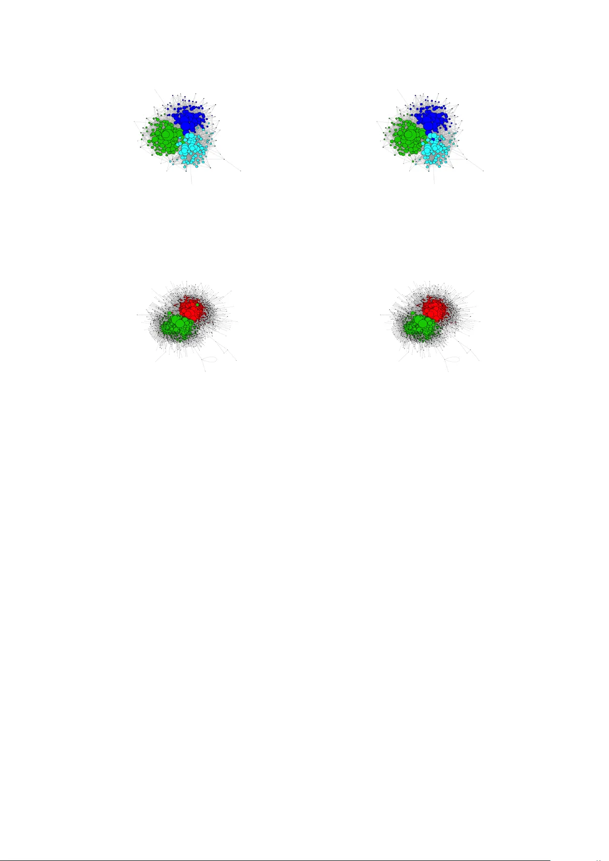
Community Detection in Netw orks using Graph Dist ance Sharmo deep Bhattac haryya and P eter J. Bic k el Jan uary 27, 2014 Abstract The study of net w orks has received increased atten tion recently not only from the so cial sciences and statistics but also from physicists, computer scien tists and mathematicians. One of the principal problem in net works is comm unity detection. Many algorithms ha ve been prop osed for communit y ﬁnding [37] [44] but most of them do not hav e hav e theoretical guaran tee for sparse netw orks and netw orks close to the phase transition b oundary prop osed b y ph ysicists [18]. There are some exceptions but all ha ve incom- plete theoretical basis [16] [14] [29]. Here w e prop ose an algorithm based on the graph distance of vertices in the netw ork. W e give theoretical guar- an tees that our metho d works in iden tifying comm unities for block mo dels, degree-corrected block mo dels [25] and blo ck mo dels with the num b er of comm unities growing with num b er of v ertices. Despite fa vorable sim ulation results, we are not y et able to conclude that our metho d is satisfactory for w orst p ossible case. W e illustrate on a netw ork of p olitical blogs, F acebo ok net works and some other netw orks. 1 In tro duction The study of netw orks has received increased atten tion recen tly not only from the so cial sciences and statistics but also from physicists, computer scientists and mathematicians. With the information b o om, a huge num b er of netw ork data sets ha ve come in to prominence. In biology - gene transcription net- w orks, protein-protein interaction netw ork, in so cial media - F aceb o ok, Twitter, Link edin netw orks, information netw orks arising in connection with text mining, tec hnological netw orks such as the In ternet, ecological and epidemiological net- w orks and man y others ha v e app eared. Although the study of netw orks has a long history in physics, social sciences and mathematics literature and informal metho ds of analysis hav e arisen in many ﬁelds of application, statistical inference on netw ork mo dels as opp osed to descriptive statistics, empirical mo deling and some Bay es ian approaches [39] [28] [23] has not b een addressed extensively in 1 the literature. A mathematical and systematic study of statistical inference on net work models has only started in recent y ears. One of the fundamen tal questions in analysis of such data is detecting and model- ing communit y structure within the net work. A lot of algorithmic approaches to comm unity detection ha ve b een prop osed, particularly in the physics and com- puter science literature [41] [36] [20]. In terms of comm unity detection, there are t wo diﬀeren t goals that researchers ha ve tried to pursue - • Algorithmic Goal: Iden tify the comm unit y eac h v ertex of the netw ork b elongs to. • Theoretical Goal: If the netw ork is generated by an underlying genera- tiv e mo del, then, what is the probability of success for the algorithm. 1.1 Algorithms Sev eral p opular algorithms for comm unity detection ha ve b een proposed in ph ysics, computer science and statistics literature. Most of these algorithms sho w decent p erformance in communit y detection for selected real-w orld and sim ulated net works [30] and ha ve p olynomial time complexity . W e shall brieﬂy men tion some of these algorithms. 1. Mo dularit y maximizing metho ds [42]. One of the most p opular metho d of comm unity detection. The problem is NP hard but spectral relaxations of p olynomial complexit y exist [40]. 2. Hierarc hical clustering techniques [15]. 3. Sp ectral clustering based metho ds [37] [16], [44] [13]. These methods are also very popular. Most of the time these metho ds ha ve linear or p olyno- mial running times. Mostly sho wn to work for dense graphs only . 4. Proﬁle likelihoo d maximization [7]. The problem is NP hard, but heuristic algorithms hav e been proposed, which hav e goo d performance for dense graphs. 5. Sto c hastic Mo del based metho ds: • MCMC based lik eliho o d maximization by Gibbs Sampling, the ca vity metho d and belief propagation based on sto chastic block mo del. [18] • V ariational Likelihoo d Maximization based on sto c hastic blo ck mo del [11], [6]. P olynomial running time but appears to w ork only for dense graphs. 2 • Pseudo-lik eliho o d Maximization [14]. F ast metho d which works well for b oth dense and sparse graphs. But the metho d is not fully justi- ﬁed. • Mo del-based: (a) Mixed Membership Blo ck Mo del [2]. Iterativ e metho d and works for dense graphs. The algorithm for this mo del is based on v ari- ational appro ximation of the maximum lik eliho o d estimation. (b) Degree-corrected blo c k mo del [25]: Incorp orates degree inhomo- geneit y in the mo del. Algorithms based on maximum likelihoo d and proﬁle lik eliho o d estimation has b een developed. (c) Ov erlapping sto c hastic blo c k mo del [31]: Stochastic block model where eac h vertex can lie within more than one comm unit y . The algorithm for this mo del is based on v ariational approximation of the maxim um likelihoo d estimation. (d) Mixed conﬁgurations model [4]: Another extension to degree- corrected sto c hastic blo c k mo del, where, the mo del is a mixture of conﬁgurations mo del (degree-corrected blo c k mo del with one blo c k) and each vertex can lie in more than one communit y . The algorithm for this mo del is based on the EM algorithm and max- im um likelihoo d estimation. 6. Mo del based clustering [22]. 1.2 Theoretical Goal The sto c hastic blo ck model (SBM) is p erhaps the most commonly used and b est studied mo del for comm unity detection. An SBM with Q blo c ks states that eac h no de b elongs to a communit y c = ( c 1 , . . . , c n ) ∈ { 1 , . . . , Q } which are dra wn in- dep enden tly from the multinomial distribution with parameter π = ( π 1 , . . . , π Q ), where π i > 0 for all i , and Q is the num b er of communities, assumed known. Conditional on the lab els, the edge v ariables A ij for i < j are indep endent Bernoulli v ariables with E [ A ij | c ] = P c i c j , (1) where P = [ P ab ] and K = [ K ab ] are Q × Q symmetric matrix. P can be consid- ered the c onne ction pr ob ability matrix, where as K is the kernel matrix for the connection. So, we ha ve P ab ≤ 1 for all a, b = 1 , . . . , Q , P 1 ≤ 1 and 1 T P ≤ 1 elemen t-wise. The netw ork is undirected, so A j i = A ij , and A ii = 0 (no self- lo ops). The problem of comm unity detection is then to infer the no de labels 3 c from A . Th us we are not really interested in estimation or inference on pa- rameters π and P , but, rather w e are interested in estimating c . But, it do es not mean the t wo problems are mutually exclusive. In realit y , the inferen tial problem and the communit y detection problem are quite interlink ed. The theoretical results of communit y detection for sto chastic blo ck mo dels can b e divided in to 3 diﬀerent regimes - (a) E ( degree ) log n → ∞ , equiv alen t to, P [there exists an isolated p oint] → 0. (b) E (degree) → ∞ , which means existence of gian t component, but also pres- ence of isolated small comp onents from Theorem 2.7. (c) If E (degree) = O (1), phase boundaries exist, b elo w whic h comm unity iden- tiﬁcation is not p ossible. Note: (a) All of the ab o ve men tioned algorithms perform satisfactorily on regime (a). (b) None of the ab ov e algorithms hav e b een shown to hav e near p erfect proba- bilit y of success under either regime (b) or (c), for the full parameter space. Some algorithms like [16] [7] [13] [14] are shown to partially w ork in the sparse setting. Some v ery recent algorithms include [29] [43]. In this pap er, w e shall only concen trate on stochastic block mo dels. In the future, w e shall try to extend our metho d and results for more general mo dels. 1.3 Con tributions and Outline of the Chapter In real life net w orks, most of the time we seem to see mo derately sparse net w orks [33] [34] [35]. Most of the large or small complex netw orks w e see seem to fall in the (b) regime of Section 1.2 w e describ e before, that is, E (degree) → ∞ . W e prop ose a simple algorithm, whic h performs w ell in practice in both regimes (b) and (c) and has some theoretical bac king If degree distribution can iden tify block parameters then classiﬁcation using our metho d should giv e reasonable result in practice. Our algorithm is based on graph distance betw een vertices of the graph. W e p erform sp ectral clustering based on the graph distance matrix of the graph. By lo oking at the graph distance matrix instead of adjacency matrix for sp ectral clustering increases the performance of the comm unity detection, as the normal- ized distance betw een cluster centers increases when w e go from the adjacency matrix to the graph distance matrix. This helps in communit y detection even for sparse matrices. W e only show theoretical results for sto chastic blo ck mo d- els. The theoretical pro ofs are quite intricate and in volv e careful coupling of 4 the stochastic block mo del with multi-t yp e branching pro cess to ﬁnd asymp- totic distribution of the t ypical graph distances. Then, a careful analysis of the eigen vector of the asymptotic graph distance matrix reveals the existence of sep- aration needed for sp ectral clustering to succeed. This metho d of analysis has b een used for sp ectral clustering analysis using the adjacency matrix also [46], but the analysis is simpler. The rest of the paper is organized as follo ws. W e giv e a summary of the prelim- inary results needed in Section 2. W e present the algorithms in Section 3. W e giv e an outline of pro of of theoretical guarantee of performance of the metho d and then the details in Section 4. The n umerical performance of the methods is demonstrated on a range of sim ulated netw orks and on some real w orld netw orks in Section 5. Section 6 concludes with discussion, and the App endix con tains some additional tec hnical results. 2 Preliminaries Let us suppose that w e hav e a random graph G n as the data. Let V ( G n ) = { v i , . . . , v n } denote the v ertices of G n and E ( G n ) = { e 1 , . . . , e m } denote the edges of G n . So, the num b er of v ertices in G n is | V ( G n ) | = n and n umber of edges of G n is | E ( G n ) | = m . Let the adjacency matrix of G n b e denoted b y A n × n . F or the sake of notational simplicity , from here onw ards we shall denote G n b y G ha ving n v ertices unless sp eciﬁcally men tioned. W e consider the n v ertices of G are clustered into Q diﬀeren t communities w ith eac h communit y ha ving size n a , a = 1 , . . . , Q and P a n a = n . In this pap er, we are interested in the problem of vertex c ommunity identiﬁc ation or gr aph p artitioning . That means that w e are interested in ﬁnding whic h of the Q diﬀeren t communit y eac h vertex of G b elongs to. Ho w ever, the problem is an unsup ervise d le arning problem. So, we assume that the data is coming from an underlying mo del and we try to verify ho w go o d ‘our’ c ommunity dete ction metho d w orks for that mo del. 2.1 Mo del for Communit y Detection As a mo del for communit y detection, we consider the sto c hastic blo ck mo del. W e shall deﬁne the sto chastic blo ck mo del shortly , but, w e ﬁrst w e shall intro- duce some more general models, of which sto chastic blo ck mo del is a sp ecial case. 5 2.1.1 Bic k el-Chen Mo del The general non-parametric mo del, as described in Bick el, Chen and Levina (2011) [8], that generates the random data netw ork G can b e deﬁned by the follo wing equation - P( A ij = 1 | ξ i = u, ξ j = v ) = h n ( u, v ) = ρ n w ( u, v ) 1 ( w ≤ ρ − 1 n ) , (2) where, w ( u, v ) ≥ 0, symmetric, 0 ≤ u, v ≤ 1, ρ n → 0. F or blo c k mo dels, the laten t v ariable for eac h vertex ( ξ 1 , . . . , ξ n ) can b e considered to b e coming from a discrete and ﬁnite set. Then, eac h elemen t of that set can b e considered to b e inducing a partition in the vertex set V ( G n ). Th us, w e get a mo del for vertex partitioning, where, the set of vertices can be partitioned in to ﬁnite num b er of disjoin t classes, but ho wev er the partition to which each vertex b elongs to is the latent v ariable in the mo del and thus unkno wn. The main goal becomes estimating this laten t v ariable. 2.1.2 Inhomogeneous Random Graph Mo del The inhomogeneous random graph mo del (IRGM) w as introduced in Bollob´ as et. al. (2007) [9]. Let S b e a separable metric space equipped with a Borel probabilit y measure µ . F or most cases S = (0 , 1] with µ Leb esgue measure, that means a U (0 , 1) distribution. The “kernel” κ will b e a symmetric non-negative function on S × S . F or eac h n we hav e a deterministic or random sequence x = ( x 1 , . . . , x n ) of p oin ts in S . W riting δ x for the measure consisting of a point mass of w eight 1 at x , and ν n ≡ 1 n n X i =1 δ x i for the empirical distribution of x , it is assumed that ν n con verges in probabilit y to µ as n → ∞ , with conv ergence in the usual space of probability measures on S . One example where the conv ergence holds is the random case, where the x i are indep enden t and identically distributed on S with distribution µ con vergence in probabilit y holds b y the law of large n umbers. Of course, w e do not need ( x n ) n ≥ 1 to b e deﬁned for every n , but only for an inﬁnite set of in tegers n . F rom here on wards, we shall only focus on this sp ecial case, where, ( x 1 , . . . , x n ) iid ∼ µ . Deﬁnition 2.1. A kernel κ n on a gr ound sp ac e ( S , µ ) is a symmetric non- ne gative (Bor el) me asur able function on S × S . κ is also c ontinuous a.e. on S × S . By a kernel on a vertex sp ac e ( S , µ, ( x n ) n ≥ 1 ) we me an a kernel on ( S , µ ) . Giv en the (random) sequence ( x 1 , . . . , x n ), we let G ( n, κ ) b e the random graph G ( n, ( p ij )) with p ij ≡ min { κ ( x i , x j ) /n, 1 } . (3) 6 In other w ords, G V ( n, κ ) has n vertices { 1 , . . . , n } and, giv en x 1 , . . . , x n , an edge ij (with i 6 = j ) exists with probability p ij , indep endently of all other (unordered) pairs ij . Based on the graph k ernel we can also deﬁne an integral op erator T κ in the follo wing wa y Deﬁnition 2.2. The inte gr al op er ator T κ : L 2 ( S ) → L 2 ( S ) c orr esp onding to G ( n, κ ) , is deﬁne d as T κ f ( x )( · ) = Z 1 0 κ ( x, y ) f ( y ) dµ ( y ) , wher e, x ∈ S and any me asur able function f ∈ L 1 ( S ) . The random graph G ( n, κ ) dep ends not only on κ but also on the choice of x 1 , . . . , x n . The freedom of choice of x i in this mo del giv es some more ﬂexibility than Bick el-Chen mo del. The asymptotic b ehavior of G ( n, κ ) dep end very m uc h on S and µ . Many of these k ey results such as existence of giant comp onen t, t ypical distance, phase transition prop erties are prov ed in [9]. W e shall use these results on inhomogeneous random graphs in order to prov e results on graph distance for sto c hastic blo ck models. Here is further comparison of the Inhomogeneous random graph mo del (IR GM) with the Bick el-Chen model (BCM), to understand their similarities and dissim- ilarities - (a) In BCM, ( ξ 1 , . . . , ξ n ) iid ∼ U (0 , 1) are the latent v ariables asso ciated with the v ertices ( v 1 , . . . , v n ) of random graph G n . Similarly , in IRGM, ( x 1 , . . . , x n ) ∼ µ are the laten t v ariables asso ciated with the v ertices ( v 1 , . . . , v n ) of ran- dom graph G n . Now, if in IR GM, ( x 1 , . . . , x n ) iid ∼ µ then the laten t v ariable structure of the tw o mo dels b ecome equiv alent. (b) In BCM, the conditional probabilit y of connection betw een t wo vertices giv en the v alue of their laten t v ariables is con trolled by the kernel function h n ( u, v ). In IR GM, the conditional probabilit y of connection b et ween t wo v ertices giv en the v alue of their laten t v ariables is controlled b y the k ernel function κ ( u,v ) n . (c) So, if h n ( u, v ) = κ ( u, v ) /n , S [(0 , 1) and the underlying measure spaces are same and the measure µ is a uniform measure on in terv al S = (0 , 1), then, BCM and IRGM generates graphs from the same distribution. In fact, as noted in [7], if S = R and µ has a p ositive densit y with resp ect to Leb esgue measure, then the (limiting) IR GM is equiv alent to Bick el-Chen mo del with suitable h n . (d) F or IR GM, let us deﬁne λ ≡ || T κ || ≡ sup f ∈ L 2 ( S ) , || f || L 2 ( S ) =1 Z S Z S κ ( u, v ) f ( u ) f ( v ) dµ ( u ) dµ ( v ) , 7 where, T κ is the op erator deﬁne in Deﬁnition 2.2 and || · || is the op erator norm. In BCM, ρ n ≡ Z 1 0 Z 1 0 h n ( u, v ) dudv . If BCM and IRGM ha ve same underlying measure spaces ( S = (0 , 1) , µ = U (0 , 1)) and h n ( u, v ) = κ ( u, v ) /n and Case 1: 1 is the principal eigenfunction of T κ , then nρ n → λ where, λ is as deﬁned ab ov e. Case 2: 1 is not the principal eigenfunction of T κ , then nρ n ≤ λ In case of BCM nρ n is the natural scaling parameter for the random graph, since, E [Num b er of Edges in G n ] = 1 2 nρ n . In case of IR GM, λ is ﬁxed. How ever, w e shall see that the limiting b ehavior of the graph distance b etw een tw o vertices of the netw ork b ecomes dep endent on the parameter λ . So, the parameter λ still remains of imp ortance. W e shall henceforth fo cus on IRGM, with parameter of imp ortance b eing λ 2.1.3 Sto c hastic Blo c k Mo del The stochastic blo c k model is p erhaps the most commonly used and b est studied mo del for comm unit y detection. W e con tinue with IRGM framework, so the graph is sparse. Deﬁnition 2.3. A gr aph G Q ( , ( P , π )) gener ate d fr om sto chastic blo ck mo del (SBM) with Q blo cks and p ar ameters P ∈ (0 , 1) Q × Q and π ∈ (0 , 1) Q c an b e deﬁne d in fol lowing way - e ach vertex of gr aph G n fr om an SBM b elongs to a c ommunity c = ( c 1 , . . . , c n ) ∈ { 1 , . . . , Q } which ar e dr awn indep endently fr om the multinomial distribution with p ar ameter π = ( π 1 , . . . , π Q ) , wher e π i > 0 for al l i . Conditional on the lab els, the e dge variables A ij for i < j ar e indep endent Bernoul li variables with E [ A ij | c ] = P c i c j = min { K c i c j n , 1 } , (4) wher e P = [ P ab ] and K = [ K ab ] ar e Q × Q symmetric matric es. P is known as the c onne ction pr ob ability matrix and K as the kernel matrix for the c onne ction. So, we have P ab ≤ 1 for al l a, b = 1 , . . . , Q , P 1 ≤ 1 and 1 T P ≤ 1 element-wise. 8 The netw ork is undirected, so A j i = A ij , and A ii = 0 (no self-lo ops). The problem of comm unit y detection is then to infer the node labels c from A . Th us w e are not really interested in estimation or inference on parameters π and P , but, rather we are in terested in estimating c . But, it does not mean the t wo problems are mutually exclusiv e, in reality , the inferen tial problem and the comm unity detection problem are quite in terlink ed. W e can see that SBM is a special case of b oth Bick el-Chen model and IR GM. In IR GM, if we consider S to be a ﬁnite set, ( x 1 , . . . , x n ) ∈ [ Q ] n ([ Q ] = { 1 , . . . , Q } ) with x i iid ∼ M ul t ( n, π ) and k ernel κ : [ Q ] → [ Q ] as κ ( a, b ) = K ab ( a, b = 1 , . . . , Q ), then the resulting IR GM graph follo ws sto c hastic blo ck mo del. So, for SBM w e can deﬁne an inte gr al op er ator on [ Q ] with measure { π 1 , . . . , π Q } . Deﬁnition 2.4. The inte gr al op er ator T K : ` 1 ( S ) → ` 1 ( S ) c orr esp onding to G Q ( n, ( P , π )) , is deﬁne d as ( T K ( x )) a = Q X b =1 K ab π b x b , for a = 1 , . . . , Q wher e, x ∈ R Q . The sto chastic blo ck mo del has deep connections with Multi-type branching pro cess, just as, Ero d¨ os-R´ en yi random graph mo del (ERR GM) has connections with the branc hing pro cess. Let us introduce branching process ﬁrst. 2.2 Multi-t yp e Branc hing Pro cess W e shall try to link net work formed by SBM with the tree net w ork generated b y m ulti-t yp e Galton-W atson branch ing pro cess. In our case, the Multi-t yp e branc hing process (MTBP) has t yp e space S = { 1 , . . . , Q } , where a particle of t yp e a ∈ S is replaced in the next generation b y a set of particles distributed as a Poisson process on S with in tensity ( K ab π b ) Q b =1 . W e denote this branching pro cess, started with a single particle of type a , by B K,π ( a ). W e write B K,π for the same pro cess with the t yp e of the initial particle random, distributed according to π . Deﬁnition 2.5. (a) Deﬁne ρ k ( K, π ; a ) as the pr ob ability that the br anching pr o c ess B K,π ( a ) has a total p opulation of exactly k p articles. (b) Deﬁne ρ ≥ k ( K, π ; a ) as the pr ob ability that the total p opulation is at le ast k . (c) Deﬁne ρ ( K , π ; a ) as the pr ob ability that the br anching pr o c ess survives for eternity. 9 (d) Deﬁne, ρ k ( K, π ) ≡ Q X a =1 ρ k ( K, π ; a ) π a , ρ ≡ ρ ( K , π ) ≡ Q X a =1 ρ ( K, π ; a ) π a (5) and deﬁne ρ ≥ k ( K ) analo gously. Thus, ρ ( K, π ) is the survival pr ob ability of the br anching pr o c ess B K,π given that its initial distribution is π If the probabilit y that a particle has inﬁnitely man y c hildren is 0, then ρ ( K, π ; a ) is equal to ρ ∞ ( a ), the probability that the total p opulation is inﬁnite. As we shall see later, the branc hing pro cess B K,π ( a ) arises naturally when exploring a comp onen t of G n starting at a vertex of t yp e a ; this is directly analogous to the use of the single-type P oisson branc hing pro cess in the analysis of the Erd¨ os-R ´ enyi graph G ( n, c/n ). 2.3 Kno wn Results for Sto chastic Blo c k Mo del The p erformance of communit y detection algorithms dep ends on the parameters π and P . W e refer to Deﬁnition 2.3 for deﬁnition of sto chastic block models. An imp ortan t condition that we usually put on parameter P is irr e ducibility . Deﬁnition 2.6. A c onne ction matrix P on a S = { 1 , . . . , Q } is r e ducible if ther e exists A ⊂ S with 0 < | A | < Q such that P = 0 a.e. on A × ( S − A ) ; otherwise P is irr e ducible . Thus P is irr e ducible if A ⊆ S and P = 0 a.e. on A × ( S − A ) implies | A | = 0 or | A | = Q . So, the results on existence of gian t comp onents in [9] also apply for SBM. The follo wing theorem describ es the result on existence of gian t comp onents. Theorem 2.7 ([9]) . L et us deﬁne op er ator T K as in deﬁnition 2.4, (i) If || T K || ≤ 1 ( || · || r efer to op er ator norm), then the size of lar gest c om- p onent is o P ( n ) , while if || T K || > 1 , then the size of lar gest c omp onent is Θ P ( n ) whp. (ii) If P is irr e ducible, then 1 n ( Size of lar gest c omp onent ) → π T ρ , wher e, ρ ∈ [0 , 1] Q is the survival pr ob ability as deﬁne d in (5) . The theoretical results on communit y detection dep end on the 3 diﬀerent regime on whic h the generative model is based on - (a) E ( degree ) log n → ∞ , equiv alent to, P [there exists an isolated p oint] → 0. In this setting, there are sev eral algorithms, suc h as those describ ed in Section 1, can identify correct communit y with high probability under quite relaxed conditions on parameters P and π . See [13] (Theorem 2 and 3), [44] (Theorem 3.1), [16] (Theorem 1). 10 (b) E (degree) → ∞ , which means existence of gian t component, but also pres- ence of isolated small comp onen ts from Theorem 2.7. In this setting, al- gorithms prop osed in [16], [14] is prov ed to iden tify comm unit y labels that are highly correlated with original communit y lab els with high probability . (c) If E (degree) = O (1), phase boundaries exist, b elo w whic h comm unity iden- tiﬁcation is not possible. These results and rigorous pro of are given in [38]. The results can b e summarized for 2-blo ck mo del with parameters P 11 = a, P 12 = b, P 22 = a as Theorem 2.8 ([38]) . (i) If ( a − b ) 2 < 2( a + b ) then pr ob ability mo del of SBM and ERR GM with p = a + b 2 n ar e mutual ly c ontiguous. Mor e over, if ( a − b ) 2 < 2( a + b ) , ther e exists no c onsistent estimators of a and b . (ii) If ( a − b ) 2 > 2( a + b ) then pr ob ability mo del of SBM and ERRGM with p = a + b 2 n ar e asymptotic al ly ortho gonal. So, in the range ( a − b ) 2 > 2( a + b ), there should exists an algorithm which iden tiﬁes highly correct clustering with high probability at least within the gian t comp onents. 3 Algorithm The algorithm we prop ose dep end on the graph distance or geodesic distance b et ween v ertices in a graph. Deﬁnition 3.1. Gr aph distanc e or Ge o desic distanc e b etwe en two vertic es i and j of gr aph G is given by the length of the shortest p ath b etwe en the vertic es i and j , if they ar e c onne cte d. Otherwise, the distanc e is inﬁnite. So, for an y tw o vertices u, v ∈ V ( G ), graph distance, d g is deﬁned b y d g ( u, v ) = ( | V ( e ) | , if e is the shortest path connecting u and v ∞ , u and v are not connected F or sak e of n umerical con v enience, w e shall replace ∞ by a large n umber for v alue of d g ( u, v ), when, u and v are not connected. The main steps of the algorithm can b e describ ed as follo ws 1. Find the graph distance matrix D = [ d g ( v i , v j )] n i,j =1 for a given net work but with distance upper b ounded b y k log n . Assign non-connected vertices an arbitrary high v alue B . 2. P erform hierarc hical clustering to identify the giant comp onen t G C of graph G . Let n C = | V ( G C ) | . 11 3. Normalize the graph distance matrix on G C , D C b y ¯ D C = −  I − 1 n C 11 T  ( D C ) 2  I − 1 n C 11 T  4. P erform eigenv alue decomposition on ¯ D C . 5. Consider the top Q eigenv ectors of normalized distance matrix ¯ D C and ˜ W b e the n × Q matrix formed by arranging the Q eigen vectors as columns in ˜ W . P erform Q -means clustering on the rows ˜ W , that means, ﬁnd an n × Q matrix C , which has Q distinct ro ws and minimizes || C − ˜ W || F . 6. (Alternativ e to 5.) Perform Gaussian mixture mo del based clustering on the ro ws of ˜ W , when there is an indication of highly-v arying av erage degree b et ween the comm unities. 7. Let ˆ ξ : V 7→ [ Q ] b e the blo c k assignmen t function according to the cluster- ing of the rows of ˜ W p erformed in either Step 5 or 6. Here are some imp ortan t observ ations ab out the algorithm - (a) There are standard algorithms for graph distance ﬁnding in the algorith- mic graph theory literature. In algorithmic graph theory literature the problem is kno wn as the all pairs shortest path problem. The t wo most p opular algorithms are Floyd-W arshall [19] [48] and Johnson’s algo- rithm [24]. The time complexity of the Flo yd-W arshall algorithm is O ( n 3 ), where as, the time complexit y of Johnson’s algorithm is O ( n 2 log n + ne ) [32] ( n = | V ( G n ) | and e = | E ( G n ) | ). So, for sparse graphs, Johnson’s algorithm is faster than Floyd-W arshall. Memory storage is also another issue for this algorithm, since the algorithm in v olves a matrix multiplica- tion step of complexity Ω( n 2 ). Recently , there also has b een some progress on parallel implementation of all-pairs shortest path problem [45] [10] [21], whic h addresses b oth memory and computation asp ects of the algorithm and lets us scale the algorithm for large graphs, b oth dense and sparse. (b) The Step 3 of the algorithm is nothing but the classical multi-dimensional scaling (MDS) of the graph distance matrix. In MDS, we try to ﬁnd v ectors ( x 1 , . . . , x n ), where, x i ∈ R Q , suc h that, n X i,j =1  || x i − x j || 2 − ( D C ) ij  2 is minimized. The minimizer is attained b y the ro ws of the matrix formed b y the top Q eigen vectors of ¯ D C as columns. So, p erforming sp ectral clustering on ¯ D C is the same as p erforming Q -means clustering on the m ulti-dimensional scaled space. 12 Instead of ¯ D C , w e could also use the matrix ( D C ) 2 , but then, the topmost eigen vector do es not carry an y information ab out the clustering. Similarly , w e can also use the matrix D C directly for spectral clustering, but, in that case, D C is not a positive semi-deﬁnite matrix and as a result w e ha ve to consider the eigenv ectors corresp onding to largest absolute eigen v alues (since eigen v alues can b e negative). (c) In the Step 5 of the algorithm Q -means clustering if the exp ected degree of the blo c ks are equal. How ever, if the exp ected degree of the blo cks are diﬀeren t, it leads to multi scale b ehavior in the eigenv ectors of the nor- malized distance matrix. So, we perform Gaussian Mixture Mo del (GMM) based clustering instead of Q -means to tak e in to accoun t the multi scale b eha vior. 4 Theory Let us consider that we hav e a random graph G n as the data. Let V ( G n ) = { v i , . . . , v n } denote the vertices of G n and E ( G n ) = { e 1 , . . . , e m } denote the edges of G n . So, the num b er of v ertices in G n is | V ( G n ) | = n and n umber of edges of G n is | E ( G n ) | = m . Let the adjacency matrix of G n b e denoted by A n × n . F or sake of notational simplicit y , from here on wards we shall denote G n b y G having n vertices unless speciﬁcally men tioned. There are Q comm unities for the v ertices and each communit y has ( n a ) Q a =1 n umber of vertices. In this pap er, w e are interested in the problem of vertex c ommunity identiﬁc ation or gr aph p artitioning . Ho wev er, the problem is an unsup ervise d le arning problem. So, w e assume that the data is coming from an underlying mo del and w e try to v erify ho w goo d ‘our’ c ommunity dete ction metho d w orks for that mo del. The theoretical analysis of the algorithm has tw o main parts - I. Finding the limiting distribution of graph distance b etw een tw o typical v ertices of type a and type b (where, a, b = 1 , . . . , Q ). This part of the analysis is highly dep enden t on results from multi-t yp e branc hing processes and their relation with sto chastic blo ck mo dels. The proof tec hniques and results are b orro wed from [9], [5] and [3]. I I. Finding the b ehavior of top Q eigenv ectors of the graph distance matrix D using the limiting distribution of the t ypical graph distances. This part of analysis is highly dependent on p erturbation theory of linear operators. The pro of tec hniques and results are b orrow ed from [26], [12] and [46]. 13 4.1 Results of Part I W e shall give limiting results for typic al distanc e betw een vertices in G n . If u and v ∈ V ( G n ) are tw o v ertices in G n , which has b een selected uniformly at random from type a and t yp e b resp ectively , where, a, b = 1 , . . . , Q are the diﬀeren t communities. Then, the graph distance b et ween u and v is d G ( u, v ). No w, the op erator that con trols the pro cess is T K as deﬁned in Deﬁnition 2.4. T K is another represen tation of the matrix ˜ K Q × Q , whic h is deﬁned as ˜ K ab ≡ π a K ab π b , for a, b = 1 , . . . , Q (6) The matrix ˜ K deﬁnes the quadratic form for T K : ` 1 ( S , π ) → ` 1 ( S , π ). So, w e ha ve that λ ≡ || T K || = λ max ( ˜ K ) . (7) The relation b etw een λ and E [num b er of Edges in G n ] is given Section 2.1.2. Here, we use λ as the scaling op erator, not either av erage, minimum or maxi- m um degree of vertices as used in [46] and [44]. But, w e already kno w that, if the graph is homo gene ous , then, E [n umber of Edges in G n ] = 1 2 λ and otherwise E [n umber of Edges in G n ] ≤ λ . Let us also denote, ν ∈ R Q as the eigenv ector of ˜ K corresp onding to λ . W e at ﬁrst, try to ﬁnd an asymptotic b ound on the graph distance d G ( u, v ) for v ertices u, v ∈ V ( G ). Theorem 4.1. L et λ > 1 (deﬁne d in Eq. (7) ), then, the gr aph distanc e d G ( u, v ) b etwe en two uniformly chosen vertic es of typ e a and b r esp e ctively, c onditione d on b eing c onne cte d, satisﬁes the fol lowing asymptotic r elation - (i) If a = b P  d G ( u, v ) ≤ (1 − ε ) log n log( π a K aa )  = o (1) (8) P  d G ( u, v ) ≥ (1 + ε ) log nπ a log( π a K aa )  = o (1) (9) (ii) If a 6 = b , P  d G ( u, v ) ≤ (1 − ε ) log n log | λ |  = o (1) (10) P  d G ( u, v ) ≥ (1 + ε ) log n log | λ |  = o (1) (11) No w, let us consider the limiting op erator D deﬁned as 14 Deﬁnition 4.2. The normalize d limiting matrix is an n × n matrix, D , which in limit as n → ∞ b e c omes an op er ator on l 2 (sp ac e of c onver gent se quenc es), is deﬁne d as D = [ D ij ] n i,j =1 , wher e, D ij = ( 1 log | λ | , if typ e of v i = a 6 = b = typ e of v j 1 log( π a K aa ) , if typ e of v i = typ e of v j = a and D ii = 0 for al l i = 1 , . . . , n . The gr aph distanc e matrix D c an b e deﬁne d as D = [ d ( v i , v j )] n i,j =1 . In Theorem 4.1 we had a p oint-wise result, so, we combine these p oin t-wise results to giv e a matrix result - Theorem 4.3. L et λ = || T K || > 1 , then, within the big c onne cte d c omp onent, P          D log n − D         F ≤ O ( n 1 − ε )  = 1 − o (1) Th us, the ab o v e theorem gives us an idea about the limiting b eha vior of the normalized v ersion of geo desic matrix D . 4.1.1 Sk etc h of Analysis of Part I A rough idea of the proof of part I is as follo ws. Fix tw o vertices, say 1 and 2, in the gian t comp onen t. Think of a branc hing pro cess starting from v ertices of t yp e 1 and 2, so that at time t , B P π ( a )( t ) is the branc hing pro cess tree from v ertex of t yp e a and includes the shortest paths to all v ertices in the tree at or b efore time t from v ertex a , a = 1 , 2. When these tw o trees meet via the formation of an edge ( v 1 , v 2 ) b etw een tw o v ertices v 1 ∈ B P π (1)( · ) and v 2 ∈ B P π (2)( · ), then the shortest-length path betw een the t wo v ertices 1 and 2 has been found. If D n ( v a ), a = 1 , 2, denotes the n umber of edges b et ween the source a and the v ertex v a along the tree B P π ( a ), then the graph distance d n (1 , 2) is giv en by d n (1 , 2) = D n ( v 1 ) + D n ( v 2 ) + 1 (12) The ab o ve idea is indeed a v ery rough sketc h of our pro of and it follows from the graph distance ﬁnding idea developed in [9]. In the pap er, w e em b ed the SBM in a m ulti-type branc hing process (MTMBP) or a single-type mark ed branc hing pro cess (MBP), dep ending on whether the t yp es of tw o vertices are same or not. The oﬀspring distribution is binomial with parameters n − 1 and k ernel P (see Section 4.4). With high probability , the v ertex exploration pro cess in the SBM can b e coupled with tw o multi-t yp e branching pro cesses, b ounding the vertex exploration pro cess on SBM on b oth sides. Now, using the prop ert y of the t wo 15 m ulti-type branc hing pro cesses, we can b ound the num b er of v ertices explored in the v ertex exploration process of a SBM graph and infer about the asymptotic limit of the graph distance. With the ab o ve sk etch of proof can b e organized as follo ws. 1. W e analyze v arious prop erties of a Galton-watson pro cess conditioned on non-extinction, including times to grow to a particular size. In this branc h- ing pro cess, the oﬀspring will hav e a Poisson distribution. 2. W e in tro duce m ulti-type branching pro cess trees with binomially distributed oﬀspring and make the connection b etw een these trees and the SBM. W e b ound the v ertices explored for an SBM graph, starting from a ﬁxed v ertex, b y considering a muti-t yp e branching process coupled with it. 3. W e bound the geo desic distance using the num b er of v ertices explored in the coupled m ulti-type branching pro cesses within a certain generation. The limiting b ehavior of the generation give us the limiting b ehavior of graph distance. 4. The whole analysis is true for IR GM. So, the results are true for SBM with increasing blo c k num b ers and degree-corrected blo ck models also. The idea of the argument is quite simple, but m aking these ideas rigorous tak es some technical work, particularly b ecause we need to condition on our vertices b eing in the gian t comp onent. 4.2 Results of Part I I So, from Part I of the analysis, we get an idea ab out the p oin t-wise asymptotic con vergence of the matrix D = [ d ( v i , v j )] n i,j =1 to the normalized limiting operator D , deﬁned in Deﬁnition 4.2. The limiting matrix D can also b e written in terms of limiting lo w-dimensional matrix, D , whic h is deﬁned as follows - Deﬁnition 4.4. The limiting kernel matrix, D Q × Q is deﬁne d as D ab = ( 1 log | λ | , if a 6 = b 1 log( π a K aa ) , if a = b So, we can see that if J n × n = 11 T is an n × n matrix of all ones, then, there exists a p ermutation of rows of D , whic h is obtained by m ultiplying D with p erm utation matrix R , such that, D R = D ? J − D iag ( ˜ d ) ≡ [ D ab J ab ] Q a,b =1 − D iag ( ˜ d ) (13) 16 where, [ J ab ] Q a,b =1 is a Q × Q partition of J in the following wa y - the ro ws and columns are partitioned in similar fashion according to ( n 1 , . . . , n Q ). Note t hat, ( n a ) Q a =1 are the num b er of vertices of t yp e a in the graph G n . So, J ab is an n a × n b matrix of all ones. ˜ d is a vector of length containing n a elemen ts of v alue 1 log( π a K aa ) , a = 1 , . . . , Q . Note that pro duct ? can also b e seen as a Khatri-Rao pro duct of t wo partitioned matrices [27]. No w, w e assume some conditions on the limiting low-dimensional matrix D . (C1) W e assume that λ < min a { π a K aa } , where, λ deﬁned in Eq. (7) is the principal eigenv ector of op erator T K deﬁned in Def. 2.4 or the matrix ˜ K deﬁned in Eq. (6). (C2) The eigenv alues of D , λ 1 ( D ) ≥ · · · ≥ λ Q ( D ), satisfy the condition that there exists an constant α , suc h that, 0 < α ≤ λ Q ( D ). (C3) The eigenv ectors of D , ( v 1 ( D ) , . . . , v Q ( D )) corresp onding to λ 1 , . . . , λ Q , satisfy the condition that there exists a constan t β , such that, rows of the Q × Q matrix V = [ v 1 · · · v Q ], represented as ( u 1 , . . . , u Q ) ( u a ∈ R Q ), satisﬁes the condition 0 < β ≤ || u a − u b || 2 for all pairs of rows of V . (C4) The n umber of v ertices in each t yp e ( n 1 , . . . , n Q ), satisfy the condition that there exists a constant θ such that 0 < θ < n a n for all a = 1 , . . . , Q and all n . Theorem 4.5. Under the c onditions (C1)-(C4), supp ose that the numb er of blo cks Q is known. L et ˆ ξ : V 7→ [ Q ] b e the blo ck assignment function ac c or ding to a clustering of the r ows of ˜ W ( n ) satisfying algorithm in Se ction 3 and ξ : V 7→ [ Q ] b e the actual assignment. L et P Q b e the set of p ermutations on [ Q ] . With high pr ob ability and for lar ge n it holds that min π ∈P Q |{ u ∈ V : ξ ( u ) 6 = π ( ˆ ξ ( u )) }| = O ( n 1 / 2 − ε ) (14) 4.2.1 Sk etc h of Pro of of Part I I W e can consider the limiting distribution of the graph distance matrix as D whic h w as proposed in Theorem 4.3, with ( D ij ) = d G ( v i , v j ), where, v i , v j ∈ V ( G ). Our goal is to sho w that the eigenv ectors of D or normalized version of it, conv erge to eigenv ectors of D or D . F or that reason, w e use the p erturbation theory of op erators, as giv en in Kato [26] and Davis-Kahan [17]. The steps are as follo ws • W e use Da vis-Kahan to sho w conv ergence of eigenspace ˜ W , formed b y top Q eigen vectors of D / log n to WR , where, W is the eigenspace formed by the top Q eigenv ectors of D and R is some orthogonal p erm utation matrix, whic h p ermutes the ro ws of W . 17 • W e sho w b y contradiction that if the clustering assignmen t mak es to o man y mistak es then the rate of conv ergence of ˜ W to WR would b e violated. 4.3 Branc hing Pro cess Results The branc hing process B K ( a ) is a m ulti-type Galton-W atson branc hing processes with t yp e space S ≡ { 1 , . . . , Q } , a particle of t yp e a ∈ S is replaced in the next generation by its “children”, a set of particles whose t yp es are distributed as a P oisson pro cess on S with intensit y { K ab π b } Q b =1 . Recall the parameters K ∈ R Q × Q and π ∈ [0 , 1] Q with P Q a =1 π a = 1, from the deﬁnition of Sto chastic blo c k mo del in equation (4). The zeroth generation of B K ( a ) consists of a single particle of t yp e a . Also, the branc hing pro cess B K is just the pro cess B K ( a ) started with a single particle whose (random) type is distributed according to the probabilit y measure ( π 1 , . . . , π Q ). Let us recall our notation for the surviv al probabilities of particles in B K ( a ). W e write ρ k ( K ; a ) for the probabilit y that the total p opulation consists of exactly k particles, and ρ ≥ k ( K ; a ) for the probabilit y that the total p opulation con tains at least k particles. F urthermore, ρ ( K ; a ) is the probabilit y that the branc hing pro cess survives for eternity . W e write ρ k ( K ) , ρ ≥ k ( K ) and ρ ( K ) for the corre- sp onding probabilities for B K , so that, e.g., ρ k ( K ) = P Q a =1 ρ k ( K ; a ) π a . No w, we try to ﬁnd a coupling relation b et ween neighb orho o d explor ation pr o c ess of a v ertex of t yp e a in sto c hastic blo c k mo del and m ulti-type Galton-W atson pro cess, B ( a ) starting from a vertex of t yp e a . W e assume all v e rtices of graph G n generated from a sto c hastic blo c k mo del has b een assigned a communit y or t yp e ξ i (sa y) for vertex v i ∈ V ( G n ). By neighb orho o d explor ation pr o c ess of a v ertex of type a in sto chastic blo ck mo del, w e mean that w e start from a random vertex v i of t yp e a in the random graph G n generated from sto c hastic blo ck mo del. Then, w e coun t the num b er of vertices of the random graph G n are neigh b ors of v i , N ( v i ). W e repeat the neighborho o d exploration pro cess b y looking at the neighbors of the v ertices in N ( v i ). W e con tinue until w e hav e cov ered all the vertices in G n . Since, we either consider G n connected or only the gian t comp onent of G n , the neighborho o d exploration pro cess will end in ﬁnite steps but the n umber of steps may dep end on n . Lemma 4.6. Within the giant c omp onent, the neighb orho o d explor ation pr o c ess for a sto chastic blo ck mo del gr aph with p ar ameters ( P , π ) = ( K /n, π ) , c an b e b ounde d with high pr ob ability by two multi-typ e br anching pr o c esses with kernels (1 − 2  ) K and (1 +  ) K for some  > 0 . Pr o of. The pro of is giv en in App endix A1 and follows from Lemma 9.6 [9]. 18 No w, w e restrict ourselv es to the giant component only . So, if w e condition that the exploration process do es not leav e the gian t component, it is same as conditioning that the branching pro cess do es not die out. Under this additional condition, the branc hing process can b e coupled with another branching pro cess with a diﬀeren t k ernel. The kernel of that branc hing pro cess is giv en in following lemma. Lemma 4.7. If we c ondition a br anching pr o c ess, B K π on survival, the new br anching pr o c ess has kernel ( K ab ( ρ ( K ; a ) + ρ ( K ; b ) − ρ ( K ; a ) ρ ( K ; b ))) Q a,b =1 . Pr o of. The pro of is given in App endix A2 and follows from Section 10 of [9]. No w, we shall try to pro ve the limiting behavior of t ypical distance b etw een v ertices v and w of G n , where, v , w ∈ V ( G n ). W e ﬁrst try to ﬁnd a low er bound for distance b etw een t wo vertices. W e shall separately giv e an upper bound and lo wer b ound for distance b et ween tw o v ertices of same t yp e and diﬀeren t t yp es. The result on low er b ound in prov ed in Lemma 4.8. Lemma 4.8. F or vertic es v , w ∈ V ( G ) , if (a) typ e of v = a 6 = b = typ e of w (say) and λ ≡ || T K || > 1 , then, E |{{ v , w } : d G ( v , w ) ≤ (1 − ε ) log n/ log | λ |}| = O ( n 2 − ε ) and so      { v , w } : d G ( v , w ) ≤ (1 − ε ) log n log λ      ≤ O ( n 2 − ε/ 2 ) with high pr ob ability (b) typ e of v = typ e of w = a (say), λ ≡ || T K || < π a K aa and λ > 1 , then, E |{{ v , w } : d G ( v , w ) ≤ (1 − ε ) log n/ log( π a K aa ) }| = O ( n 2 − ε ) and so      { v , w } : d G ( v , w ) ≤ (1 − ε ) log n log( π a K aa )      ≤ O ( n 2 − ε/ 2 ) with high pr ob ability Pr o of. The pro of is giv en in App endix A3 and follows from Lemma 14.2 of [9]. No w, w e ﬁrst try to upp er b ound the t ypical distance b etw een tw o v ertices of the same type. F or the same t yp e v ertices, w e just fo cus on the subgraph of the original graph from sto c hastic blo ck model having v ertices of same type. So, in Lemma 4.9, the graph G n is the subgraph of the original graph containing only the vertices of the same type. So, the coupled branching proces s on that graph automatically b ecomes a single-t yp e branching process. 19 Lemma 4.9. F or vertic es v , w ∈ V ( G ) , if typ e of v = typ e of w = a (say) P  d G ( v , w ) < (1 + ε ) log( nπ a ) log( π a K aa )  = 1 − exp ( − Ω( n 2 η )) c onditione d on the event that the br anching pr o c ess B K aa ( a ) survives. Pr o of. The pro of is giv en in App endix A4 and follows from Lemma 14.3 of [9]. No w, let us try to upp er b ound the typical distance betw een t wo vertices of diﬀeren t t yp es. So, in Lemma 4.10, the graph G n is the original graph con taining with vertices of the diﬀerent types. So, the coupled branching pro cess on that graph b ecomes a m ulti-type branching process. Lemma 4.10. L et us have λ ≡ || T K || = λ max ( ˜ K ) > 1 fr om Eq (7) . F or uni- formly sele cte d vertic es v , w ∈ V ( G ) , P  d G ( v , w ) < (1 + ε ) log n log λ  = 1 − exp ( − Ω( n 2 η )) c onditione d on the event that the br anching pr o c ess B K survives. Pr o of. The pro of is giv en in App endix A5 follows from Lemma 14.3 of [9]. 4.4 Pro of of Theorem 4.1 and Theorem 4.3 4.4.1 Pro of of Theorem 4.1 W e shall try to prov e the limiting b eha vior of typical graph distance in the gian t comp onen t as n → ∞ . The Theorem essen tially follo ws from Lemma 4.8 - 4.10. Under the conditions mentioned in the Theorem, part (a) follows from Lemma 4.8(b) and 4.9 and part (b) follows from Lemma 4.8(a) and 4.10. 4.4.2 Pro of of Theorem 4.3 F rom the deﬁnition 4.2, we ha ve that D ij = graph distance b etw een vertices v i and v j , where, v i , v j ∈ V ( G n ). Case 1: F or the case when t yp e of v i = t yp e of v j = a (sa y) F rom Lemma 4.8(b), we get for any v ertices v and w of same type a with high probabilit y ,      { v , w } : d G ( v , w ) ≤ (1 − ε ) log n log( π a K aa )      ≤ O ( n 2 − ε ) . Also from Lemma 4.9, we get, for an y vertices v and w of same type a P  d G ( v , w ) < (1 + ε ) log n log( π a K aa )  = 1 − exp ( − Ω( n 2 η )) 20 So, w e hav e that, for v i , v j ha ving same type a , with high probability ,  D ij log n − D ij  2 ≤ Constan t ε 2 Since,  = O ( n − 1 / 2 ) b y Eq (16) and (1 − exp ( − Ω( n 2 η ))) n 2 → 1 as n → ∞ , n X i,j =1: ty pe ( v i )= ty pe ( v j )  D ij log n − D ij  2 ≤ ε 2 .O (( nπ a ) 2 ) = O ( n ) with high probabilit y . Case 2: F or the case when t yp e of v i 6 = t yp e of v j F rom Lemma 4.8(a), w e get for any v ertices v and w with high probability ,      { v , w } : d G ( v , w ) ≤ (1 − ε ) log n log λ      ≤ O ( n 2 − ε ) . Also, from Lemma 4.10, we get P  d G ( v , w ) < (1 + ε ) log n log λ  = 1 − exp ( − Ω( n 2 η )) So, putting the tw o statements together, w e get that with high probability , n X i,j =1: ty pe ( v i ) 6 = ty pe ( v j )  D ij log n − D ij  2 = O ( n 2 − ε ) + O ( n 2 ) .ε 2 = O ( n 2 − ε ) since, by Eq. (16)  = O (1 / √ n ) and and (1 − exp ( − Ω( n 2 η ))) n 2 → 1 as n → ∞ . So, putting the tw o cases together, we get that with high probabilit y , n X i,j =1  D ij log n − D ij  2 = O ( n 2 − ε ) + O ( n 2 ) .ε 2 = O ( n 2 − ε ) . Hence,         D log n − D         F ≤ O ( n 1 − ε/ 2 ) . 4.5 P erturbation Theory of Linear Op erators Once, we ha ve the limiting b eha vior of the matrix D established in Theorem 4.3, w e shall now try to see the b eha vior of the eigenv ectors of the matrix D . Now, matrix D can b e considered as a p erturbation of the op erator D . The Davis-Kahan Theorem states a b ound on p erturbation of eigenspace in- stead of eigenv ector, as discussed previously . The sin θ Theorem of Davis-Kahan [17] 21 Theorem 4.11 (Da vis-Kahan (1970)[17]) . L et H , H 0 ∈ R n × n b e symmetric, supp ose V ⊂ R is an interval, and supp ose for some p ositive inte ger d that W , W 0 ∈ R n × d ar e such that the c olumns of W form an orthonormal b asis for the sum of the eigensp ac es of H asso ciate d with the eigenvalues of H in V and that the c olumns of W 0 form an orthonormal b asis for the sum of the eigensp ac es of H 0 asso ciate d with the eigenvalues of H 0 in V . L et δ b e the minimum distanc e b etwe en any eigenvalue of H in V and any eigenvalue of H not in V . Then ther e exists an ortho gonal matrix R ∈ R d × d such that || WR − W 0 || F ≤ √ 2 || H − H 0 || F δ . 4.6 Pro of of Theorem 4.5 No w, w e can try to approximate limiting op erator b y the graph distance matrix D in F robenius norm based on Theorem 4.3 of P art I. The b ehavior of the eigen v alues of the limiting op erator D can b e stated as follo ws - Lemma 4.12. The eigenvalues of D - | λ 1 ( D ) | ≥ | λ 2 ( D ) | ≥ · · · ≥ | λ n ( D ) | , c an b e b ounde d as fol lows - λ 1 ( D ) < n, | λ K ( D ) | > C n, λ Q +1 ( D ) = − min { ˜ d 1 , . . . , ˜ d Q } , . . . , λ n = − max { ˜ d 1 , . . . , ˜ d Q } (15) wher e, ˜ d , a ve ctor of length Q , is deﬁne d in Eq. (13) and the smal lest ( n − Q ) absolute eigenvalues of D ar e − ˜ d wher e − ˜ d a has multiplicity ( n a − 1) for a = 1 , . . . , Q . Pr o of. The matrix D can b e considered as a Khatri-Rao product of the matrices D and J according to equation (13). Now, there exists a constant τ such that log || T K || > τ > 0, since || T K || > 1. So, we ha v e λ 1 ( D ) < τ . So, we ha v e λ 1 ( D ) < 1 and since n a ≤ n for all a and P a n a = n . So, we ha ve λ 1 ( D ) ≤ n . No w, By Assumption (C2) and (C4), λ Q ( D ) ≥ α and n a ≥ γ n , so, λ Q ( D ) ≥ αγ n . No w, it is easy to see that the remaining eigenv alues of D is -1, since, B ? J is a rank Q matrix and its remaining eigenv alues are zero and the eigenv alues of diagonal matrix are ˜ d with ˜ d a ha ving multiplicit y ( n a ) for a = 1 , . . . , Q . Corollary 4.13. With high pr ob ability it holds that | λ Q ( D / log n ) | ≥ O ( n ) and λ Q +1 ( D / log n ) ≤ O ( n 1 − ε ) . Pr o of. By W eyl’s Inequalit y , for all i = 1 , . . . , n , || λ i ( D / log n ) | − | λ i ( D ) || ≤         D log n − D         F ≤ O ( n 1 − ε/ 2 ) ≤ O ( n 1 − ε ) So, | λ Q ( D / log n ) | ≥ O ( n ) − O ( n 1 − ε ) = O ( n ) for large n and | λ Q +1 ( D / log n ) | ≤ − 1 + O ( n 1 − ε ) = O ( n 1 − ε ). 22 No w, if we consider W is the eigenspace corresp onding to top Q absolute eigen- v alues of D and ˜ W is the eigenspace corresponding to top Q absolute eigen v alues of D . Using Da vis-Kahan Lemma 4.14. With high pr ob ability, ther e exists an ortho gonal matrix R ∈ R Q × Q such that || WR − ˜ W || F ≤ O ( n − ε ) Pr o of. The top Q eigen v alues of b oth D and D / log n lies in ( C n, ∞ ) for some C > 0. Also, the gap δ = O ( n ) b etw een top Q and Q + 1th eigenv alues of matrix D . So, no w, we can apply Davis-Kahan Theorem 4.11 and Theorem 4.3, to get that, || WR − ˜ W || F ≤ √ 2       D log n − D       F δ ≤ O ( n 1 − ε ) O ( n ) = O ( n − ε ) No w, the relationship b etw een the rows of W can b e sp eciﬁed based on Assump- tion (C3) as follows - Lemma 4.15. F or any two r ows i, j of W n × Q matrix, || u i − u j || 2 ≥ O (1 / √ n ) , if typ e of v i 6 = typ e of v j . Pr o of. The matrix D can b e considered as a Khatri-Rao product of the matrices D and J according to equation (13). Now, by Assumption (C3), we ha ve a constan t diﬀerence b etw een the rows of matrix D . So, rows of D as well as the pro jection of D into into its top Q eigenspace has diﬀerence of order O ( n − 1 / 2 ) b et ween ro ws of matrix. No w, if we consider Q -means criterion as the clustering criterion on ˜ W , then, for the Q -means minimizer centroid matrix C is an n × Q matrix with Q distinct ro ws corresp onding to the Q centroids of Q -means algorithm. By prop erty of Q -means ob jectiv e function and Lemma 4.14, with high probability , || C − ˜ W || F ≤ || WR − ˜ W || F || C − WR || F ≤ || C − ˜ W || F + || WR − ˜ W || F ≤ 2 || WR − ˜ W || F ≤ O ( n − ε ) By Lemma 4.15, for large n , w e can get constant C , suc h that, Q balls, B 1 , . . . , B Q , of radius r = C n − 1 / 2 around Q distinct rows of W are disjoint. 23 No w note that with high probability the num b er of rows i suc h that || C i − ( WR ) i || > r is at most O ( n 1 / 2 − ε ). If the statemen t do es not hold then, || C − WR || F > r.O ( n 1 / 2 − ε ) ≥ C n − 1 / 2 .O ( n 1 / 2 − ε ) = O ( n − ε ) So, we get a contradiction, since || C − WR || F ≤ O ( n − ε ). Thus, the num b er of mistak es should b e at most of order O ( n 1 / 2 − ε ). So, for eac h v i ∈ V ( G n ), if ξ i is the t yp e of v i and ˆ ξ i is the t yp e of v i as estimated from applying Q -means on top Q eigenspace of geo desic matrix D , we get that with high probabilit y , for some small 0 < ε , min π ∈P Q |{ u ∈ V : ξ ( u ) 6 = π ( ˆ ξ ( u )) }| = O ( n 1 / 2 − ε ) 5 Application W e inv estigate the empirical p erformance of the algorithm in sev eral diﬀerent setup. At ﬁrst, we use simulated net works from stochastic blo c k mo del to ﬁnd the empirical p erformance of the algorithm. Then, w e apply our metho d to ﬁnd comm unities in several real w orld net works. 5.1 Sim ulation W e simulate netw orks from sto c hastic blo c k mo dels with Q = 3 blo cks. Let w corresp ond to a Q -blo ck mo del deﬁned b y parameters θ = ( π , ρ n , S ), where π a is the probabilit y of a no de b eing assigned to blo ck a as b efore, and F ab = P( A ij = 1 | i ∈ a, j ∈ b ) = ρ n S ab , 1 ≤ a, b ≤ K. and the probability of no de i to b e assigned to blo ck a to be π a ( a = 1 , . . . , K ). 5.1.1 Equal Densit y Clusters W e consider a sto c hastic blo c k mo del with Q = 3. W e consider the parameter matrix F = 0 . 012(1 + 0 . 1 ν )( ˜ λF (1) + (1 − ˜ λ ) F (2) ), where, F (1) 3 × 3 = Diag(0 . 9 , 0 . 9 , 0 . 9) and F (2) 3 × 3 = 0 . 1 J 2 , where, J 2 is a 2 × 2 matrix of all 1’s and ν v aries from 1 to 15 to giv e netw orks of diﬀerent densit y . So, we get ρ n = π T F π . W e now, v ary ˜ λ to get diﬀerent com binations of F as well as ρ n . In the following ﬁgures, we try to see the b ehavior of mean and v ariances of the coun t statistics, as we v ary λ n as w e v ary ν . 24 Figure 1: The LHS is the p erformance of graph distance based metho d and RHS is the p erformance of Pseudolikelihoo d metho d on same generative SBM. Figure 2: The LHS is the p erformance of graph distance based metho d and RHS is the p erformance of Pseudolikelihoo d metho d on same generative SBM. 5.1.2 Unequal Densit y Clusters W e consider a sto c hastic blo c k mo del with Q = 3. W e consider the parameter matrix F = 0 . 012(1 + 0 . 1 ν )( ˜ λF (1) + (1 − ˜ λ ) F (2) ), where, F (1) 3 × 3 = Diag(0 . 1 , 0 . 5 , 0 . 9) and F (2) 3 × 3 = 0 . 1 J 2 , where, J 2 is a 2 × 2 matrix of all 1’s and ν v aries from 1 to 15 to giv e netw orks of diﬀerent densit y . So, we get ρ n = π T F π . W e now, v ary ˜ λ to get diﬀerent com binations of F as well as ρ n . In the following ﬁgures, we try to see the b ehavior of mean and v ariances of the coun t statistics, as we v ary λ n as w e v ary ν . 5.2 Application to Real Net work Data 5.2.1 F aceb o ok Collegiate Net w ork In this application, we try to ﬁnd communities for F acebo ok collegiate netw orks. The net w orks w ere presen ted in the paper b y T raud et.al. (2011) [47]. The net- w ork is formed by F acebo ok users acting as no des and if tw o F aceb o ok users are “friends” there is an edge b etw een the corresp onding no des. Along with the net- w ork structure, w e also ha ve the data on cov ariates of the no des. Eac h node has 25 Figure 3: The LHS is communit y allo cation and RHS is the one estimated b y graph distance for F acebo ok Caltech net work with 3 dorms. Figure 4: The LHS is communit y allo cation and RHS is the one estimated b y graph distance for Political W eb blogs Netw ork. co v ariates: gender, class year, and data ﬁelds that represent (using anonymous n umerical iden tiﬁers) high sc ho ol, ma jor, and dormitory residence. W e consider the net work of a sp eciﬁc college (Caltec h). W e compare the comm unities found with the dormitory aﬃliation of the no des. 5.2.2 P olitical W eb Blogs Net work This dataset on p olitical blogs was compiled b y [1] so on after the 2004 U.S. presiden tial election. The no des are blogs fo cused on US p olitics and the edges are hyperlinks b etw een these blogs. Eac h blog was manually lab eled as lib eral or conserv ativ e b y [1], and w e treat these as true communit y lab els. W e ignore directions of the hyperlinks and analyze the largest connected component of this net work, whic h has 1222 no des and the av erage degree of 27. The distribution of degrees is highly sk ewed to the righ t (the median degree is 13, and the maxim um is 351). This is a net work where the degree distribution is heavy-tailed and the graph is inhomogeneous. 26 6 Conclusion The prop osed graph distance based communit y detection algorithm giv es a v ery general w ay for communit y detection for graphs o ver a large range of densities - from v ery sparse graphs to v ery dense graphs. W e theoretically pro ve the eﬃcacy of the method under the model that the graph is generated from stochastic block mo del with ﬁxed num b er of blocks. W e prov e that the proportion of mislabeled comm unities go es to zero as the num b er of vertices n → ∞ . This result is true for graphs coming from stochastic blo ck mo del under certain conditions on the stochastic blo ck mo del parameters. These conditions are satisﬁed ab ov e the threshold of blo ck identiﬁcation for tw o blo cks as giv en in [38]. The condition (C1) of 1 not being the eigenv ector of ˜ K for our communit y iden tiﬁcation result to hold, seems to be an artiﬁcial one, as sim ulation suggests that our method is able to iden tify communities, ev en when 1 is an eigenv ector of ˜ K . W e demonstrate the empirical p erformance of the method by using b oth sim u- lated and real world net w orks. W e compare with the pseudo-likelihoo d metho d and sho w that they ha v e similar empirical p erformances. W e demonstrate the empirical p erformance b y applying the method for communit y detection in sev- eral real w orld netw orks to o. The metho d also w orks when num b er of blocks in the sto chastic blo ck mo del bro ws with n (n um b er of vertices) and for degree-corrected block mo del [25]. W e conjecture that under these models too the metho d will hav e the theoretical guaran tee of correct communit y detection. The pro of can b e obtained by using similar tec hniques that we ha ve used in this pap er. References [1] Lada A Adamic and Natalie Glance. The p olitical blogosphere and the 2004 us election: divided they blog. In Pr o c e e dings of the 3r d international workshop on Link disc overy , pages 36–43. ACM, 2005. [2] Edoardo M Airoldi, David M Blei, Stephen E Fien b erg, and Eric P Xing. Mixed mem b ership sto chastic blockmodels. The Journal of Machine L e arn- ing R ese ar ch , 9:1981–2014, 2008. [3] Krishna B A threya and Peter E Ney . Br anching pr o c esses , volume 28. Springer-V erlag Berlin, 1972. [4] Brian Ball, Brian Karrer, and MEJ Newman. Eﬃcien t and princi- pled method for detecting comm unities in netw orks. Physic al R eview E , 84(3):036103, 2011. 27 [5] Shank ar Bhamidi, Remco V an der Hofstad, and Gerard Hooghiemstra. First passage percolation on the erds-ren yi random graph. Combinatorics, Pr ob- ability & Computing , 20(5):683–707, 2011. [6] P eter Bic kel, Da vid Choi, Xiangyu Chang, and Hai Zhang. Asymptotic nor- malit y of maxim um lik eliho o d and its v ariational approximation for stochas- tic blo c kmo dels. arXiv pr eprint arXiv:1207.0865 , 2012. [7] P eter J Bick el and Aiy ou Chen. A nonparametric view of netw ork mo dels and newman–girv an and other modularities. Pr o c e e dings of the National A c ademy of Scienc es , 106(50):21068–21073, 2009. [8] P eter J Bic kel, Aiy ou Chen, and Eliza veta Levina. The metho d of mo- men ts and degree distributions for netw ork models. The A nnals of Statistics , 39(5):2280–2301, 2011. [9] B ´ ela Bollob´ as, Sv an te Janson, and Oliver Riordan. The phase transition in inhomogeneous random graphs. R andom Structur es & A lgorithms , 31(1):3– 122, 2007. [10] Aydın Bulu¸ c, John R Gilb ert, and Ceren Budak. Solving path problems on the gpu. Par al lel Computing , 36(5):241–253, 2010. [11] Alain Celisse, J-J Daudin, and Lauren t Pierre. Consistency of maximum- lik eliho o d and v ariational estimators in the sto c hastic block mo del. arXiv pr eprint arXiv:1105.3288 , 2011. [12] F ran¸ coise Chatelin. Sp e ctr al Appr oximation of Line ar Op er ators . SIAM, 1983. [13] Kamalik a Chaudh uri, F an Ch ung Graham, and Alexander Tsiatas. Spectral clustering of graphs with general degrees in the extended planted partition mo del. Journal of Machine L e arning R ese ar ch-Pr o c e e dings T r ack , 23:35–1, 2012. [14] Aiy ou Chen, Arash A Amini, Peter J Bick el, and Elizav eta Levina. Fitting communit y models to large sparse net works. arXiv pr eprint arXiv:1207.2340 , 2012. [15] Aaron Clauset, Mark EJ Newman, and Cristopher Mo ore. Finding com- m unity structure in very large netw orks. Physic al r eview E , 70(6):066111, 2004. [16] Amin Co ja-Oghlan and Andr´ e Lank a. Finding planted partitions in ran- dom graphs with general degree distributions. SIAM Journal on Discr ete Mathematics , 23(4):1682–1714, 2009. 28 [17] Chandler Davis and William Morton Kahan. The rotation of eigenv ectors b y a p erturbation. iii. SIAM Journal on Numeric al Analysis , 7(1):1–46, 1970. [18] Aurelien Decelle, Florent Krzak ala, Cristopher Mo ore, and Lenk a Zde- b oro v´ a. Asymptotic analysis of the sto chastic blo c k mo del for mo dular net works and its algorithmic applications. Physic al R eview E , 84(6):066106, 2011. [19] Rob ert W Flo yd. Algorithm 97: shortest path. Communic ations of the A CM , 5(6):345, 1962. [20] San to F ortunato. Comm unity detection in graphs. Physics R ep orts , 486(3):75–174, 2010. [21] Ma yiz B Habbal, Haris N Koutsop oulos, and Stev en R Lerman. A decomp o- sition algorithm for the all-pairs shortest path problem on massiv ely parallel computer arc hitectures. T r ansp ortation Scienc e , 28(4):292–308, 1994. [22] Mark S Handco c k, Adrian E Raftery , and Jeremy M T an trum. Mo del- based clustering for social net works. Journal of the R oyal Statistic al So ciety: Series A (Statistics in So ciety) , 170(2):301–354, 2007. [23] P eter D Hoﬀ, Adrian E Raftery , and Mark S Handcock. Latent space ap- proac hes to so cial netw ork analysis. Journal of the americ an Statistic al asso ciation , 97(460):1090–1098, 2002. [24] Donald B Johnson. Eﬃcient algorithms for shortest paths in sparse net- w orks. Journal of the A CM (JACM) , 24(1):1–13, 1977. [25] Brian Karrer and Mark EJ Newman. Sto c hastic blo c kmo dels and commu- nit y structure in netw orks. Physic al R eview E , 83(1):016107, 2011. [26] T osio Kat¯ o. Perturb ation the ory for line ar op er ators , volume 132. springer, 1995. [27] CG Khatri and C Radhakrishna Rao. Solutions to some functional equa- tions and their applications to characterization of probabilit y distributions. Sankhy¯ a: The Indian Journal of Statistics, Series A , pages 167–180, 1968. [28] Eric D Kolaczyk. Statistic al analysis of network data . Springer, 2009. [29] Floren t Krzak ala, Cristopher Mo ore, Elchanan Mossel, Jo e Neeman, Allan Sly , Lenk a Zdeb oro v´ a, and Pan Zhang. Sp ectral redemption: clustering sparse net works. arXiv pr eprint arXiv:1306.5550 , 2013. [30] Andrea Lancichinetti and Santo F ortunato. Communit y detection algo- rithms: a comparativ e analysis. Physic al r eview E , 80(5):056117, 2009. 29 [31] Pierre Latouc he, Etienne Birmel´ e, and Christophe Ambroise. Overlapping sto c hastic blo c k mo dels with application to the frenc h p olitical blogosphere. The A nnals of Applie d Statistics , 5(1):309–336, 2011. [32] Charles E Leiserson, Ronald L Rivest, Cliﬀord Stein, and Thomas H Cor- men. Intr o duction to algorithms . The MIT press, 2001. [33] Jure Lesk o vec, Jon Klein b erg, and Christos F aloutsos. Graph ev olution: Densiﬁcation and shrinking diameters. A CM T r ansactions on Know le dge Disc overy fr om Data (TKDD) , 1(1):2, 2007. [34] Jure Lesko vec, Kevin J Lang, Anirban Dasgupta, and Michael W Mahoney . Statistical prop erties of communit y structure in large s ocial and information net works. In Pr o c e e dings of the 17th international c onfer enc e on World Wide Web , pages 695–704. ACM, 2008. [35] Jure Lesko vec, Kevin J Lang, Anirban Dasgupta, and Michael W Mahoney . Comm unity structure in large netw orks: Natural cluster sizes and the ab- sence of large well-deﬁned clusters. Internet Mathematics , 6(1):29–123, 2009. [36] Jure Lesko v ec, Kevin J Lang, and Mic hael Mahoney . Empirical comparison of algorithms for net work comm unity detection. In Pr o c e e dings of the 19th international c onfer enc e on World wide web , pages 631–640. ACM, 2010. [37] F rank McSherry . Sp ectral partitioning of random graphs. In F oundations of Computer Scienc e, 2001. Pr o c e e dings. 42nd IEEE Symp osium on , pages 529–537. IEEE, 2001. [38] Elc hanan Mossel, Joe Neeman, and Allan Sly . Sto c hastic block mo dels and reconstruction. arXiv pr eprint arXiv:1202.1499 , 2012. [39] Mark Newman. Networks: an intr o duction . OUP Oxford, 2009. [40] Mark EJ Newman. Finding communit y structure in netw orks using the eigen vectors of matrices. Physic al r eview E , 74(3):036104, 2006. [41] Mark EJ Newman. Mo dularity and comm unity structure in net works. Pr o- c e e dings of the National A c ademy of Scienc es , 103(23):8577–8582, 2006. [42] Mark EJ Newman and Mic helle Girv an. Finding and ev aluating communit y structure in net works. Physic al r eview E , 69(2):026113, 2004. [43] MEJ Newman. Sp ectral communit y detection in sparse netw orks. arXiv pr eprint arXiv:1308.6494 , 2013. [44] Karl Rohe, Soura v Chatterjee, and Bin Y u. Sp ectral clustering and the high- dimensional sto chastic blo ckmodel. The Annals of Statistics , 39(4):1878– 1915, 2011. 30 [45] Edgar Solomonik, Aydın Bulu¸ c, and James Demmel. Minimizing commu- nication in all-pairs shortest paths. University of California at Berkeley, Berkeley, US , 2012. [46] Daniel L Sussman, Minh T ang, Donniell E Fishkind, and Carey E Priebe. A consisten t adjacency sp ectral em b edding for sto chastic blo c kmo del graphs. Journal of the A meric an Statistic al Asso ciation , 107(499):1119–1128, 2012. [47] Amanda L T raud, Eric D Kelsic, Peter J Mucha, and Mason A P orter. Comparing comm unity structure to c haracteristics in online collegiate social net works. SIAM r eview , 53(3):526–543, 2011. [48] Stephen W arshall. A theorem on b o olean matrices. Journal of the ACM (JA CM) , 9(1):11–12, 1962. App endix: Branching Pro cess Results A1. Pro of of Lemma 4.6 W e hav e n a v ertices of type a , a = 1 , . . . , Q , and that n a /n a.s. → π a . F rom no w on we condition on n 1 , . . . , n Q ; we ma y th us assume that n 1 , . . . , n Q are deterministic with n a /n → π a . Let ω ( n ) b e an y function suc h that ω ( n ) → ∞ and ω ( n ) /n → 0. W e call a comp onent of G n ≡ G ( n, P ) = G ( n, K/n ) big if it has at least ω ( n ) v ertices. Let B b e the union of the big comp onents, so | B | = N ≥ ω ( n ) ( G n ). Fix  > 0.W e may assume that n is so large that ω ( n ) /n <  π i and | n a /n − π a | <  π a for every a ; th us (1 −  ) π a n < n a < (1 +  ) π a n . W e ma y also assume that n > max K , as K is a function on the ﬁnite set S × S . Since, n a /n is a √ n -consisten t estimator of π a , w e get that  = O ( n − 1 / 2 ) . (16) Select a v ertex and explore its comp onen t in the usual wa y , that means looking at its neigh b ors, one vertex at a time. W e ﬁrst reveal all edges from the initial v ertex, and put all neigh b ors that we ﬁnd in a list of unexplored v ertices; we then c ho ose one of these and reveal its entire neigh b orho o d, and so on. Stop when w e ha ve found at least ω ( n ) vertices (so x ∈ B ), or when there are no unexplored v ertices left (so we ha ve found the en tire comp onent and x / ∈ B ). Consider one step in this exploration, and assume that w e are about to rev eal the neighborho o d of a vertex x of type a . Let us write n 0 b for the num b er of un used vertices of t yp e b remaining. Note that n b ≥ n 0 b ≥ n b − ω ( n ), so (1 − 2  ) π b < n 0 b /n < (1 +  ) π b (17) 31 The num b er of new neighbors of x of t yp e b has a binomial B in ( n 0 b , K ab /n ) distribution, and the n umbers for diﬀerent b are independent. The total v ariation distance betw een a binomial B in ( n, p ) distribution and the P oisson distribution with the same mean is at most p. Hence the total v ariation distance b et ween the binomial distribution abov e and the P oisson distribution P oi ( K ab n 0 b /n ) is at most K ab /n = O (1 /n ). Also, by (17), (1 − 2  ) K ab π b ≤ K ab n 0 b /n ≤ (1 +  ) K ab π b . (18) Since w e p erform at most ω ( n ) steps in the exploration, we may , with an error probabilit y of O ( ω ( n ) /n ) = o (1), couple the exploration with tw o multi-t yp e branc hing pro cesses B ((1 − 2  ) K ) and B ((1 +  ) K ) such that the ﬁrst pro cess alw ays ﬁnds at most as many new vertices of each t yp e as the exploration, and the second pro cess ﬁnds at least as many . Consequen tly , for a vertex x of t yp e a , ρ ≥ ω ( n ) ((1 − 2  ) K ; a ) + o (1) ≤ P( x ∈ B ) ≤ ρ ≥ ω ( n ) ((1 +  ) K ; a ) + o (1) . (19) Since ω ( n ) → ∞ , by Lemma 9.5 of [9], we ha v e ρ ≥ ω ( n ) ( K ; a ) → ρ ( K ; a ) for every matrix or ﬁnitary kernel K , whic h parametrizes the oﬀspring distribution of the branc hing pro cess in the sense that the num b er of oﬀsprings of t yp e b coming from a paren t of t yp e a follo ws P oi ( K ab π b ) distribution. So we can rewrite (19) as ρ ((1 − 2  ) K ; a ) + o (1) ≤ P ( x ∈ B ) ≤ ρ ((1 +  ) K ; a ) + o (1) . (20) A2. pro of of Lemma 4.7 W e need to consider certain branching pro cess exp ectations σ ( K ) and σ ≥ k ( K ) in place of ρ ( K ) and ρ ≥ k ( K ). In preparation for the proof, we shall relate ζ ( K ) to the branching pro cess B K via σ ( K ). As b efore, w e assume that K is a kernel on ( S , π ) with K ∈ L 1 . Let A b e a P oisson pro cess on S , with intensit y giv en b y a ﬁnite measure λ , so that A is a random multi-set on S . If g is a b ounded measurable function on m ulti-sets on S , it is easy to see that E ( | A | g ( A )) = X i ∈S E g ( A ∪ { i } ) λ i (21) F or details see Prop osition 10.4 of [9]. Let B ( x ) denote the ﬁrst generation of the branching pro cess B K ( x ). Th us B ( x ) is giv en b y a P oisson process on S with intensit y K ( x, y ) π x . Suppose that P b K ab π b < ∞ for ev ery a = 1 , . . . , Q , so B ( x ) is ﬁnite. Let σ ( K ; x ) denote 32 the exp ectation of | B ( x ) | 1 [ |B K ( x ) | = ∞ ], recalling that under the assumption P b K ab π b < ∞ for ev ery a , the branching process B K ( x ) dies out if and only if |B K ( x ) | < ∞ . Then Q X b =1 K xb π b − σ ( K ; x ) = E [ | B ( x ) | 1 ( B K ( x ) < ∞ )] = E   | B ( x ) | Y z ∈ B ( x ) ρ ( K ; z )   = Q X b =1 K xb (1 − ρ ( K ; b )) E   Y z ∈ B ( x ) ρ ( K ; z )   π b = Q X b =1 K xb (1 − ρ ( K ; b ))(1 − ρ ( K ; x )) π b Here the p enultimate step is from (21); the last step uses the fact that the branc hing pro cess dies out if and only if none of the children of the initial par- ticle surviv es. W riting B for the ﬁrst generation of B K conditioned on surviv al b ecomes σ ( K ) ≡ E | B | 1 [ |B K | = ∞ ] = Q X x =1 σ ( K ; x ) π x Then, in tegrating ov er x and subtracting from P a,b K ab π a π b , w e get, σ ( K ) = X a,b K ab (1 − (1 − ρ ( K ; a ))(1 − ρ ( K ; b ))) π a π b (22) So, the k ernel for the conditioned branching process b ecomes K ab ( ρ ( K ; a ) + ρ ( K ; b ) − ρ ( K ; a ) ρ ( K ; b )) (23) A3. pro of of Lemma 4.8 W e hav e S is ﬁnite, say S = { 1 , 2 , . . . , Q } . Let Γ d ( v ) ≡ Γ d ( v , G n ) denote the d -distance set of v in G n , i.e., the set of v ertices of G n at graph distance exactly d from v , and let Γ ≤ d ( v ) ≡ Γ ≤ d ( v , G n ) denote the d -neighborho o d ∪ d 0 ≤ d Γ d 0 ( v ) of v . Let 0 < ε < 1 / 10 b e arbitrary . The pro of of (20) inv olv ed ﬁrst showing that, for n large enough, the neigh b orho o d exploration pro cess starting at a given vertex v of G n with type a (chosen without insp ecting G n ) could b e coupled with the branc hing process B (1+ ε ) K 0 ( i ), where the K 0 is deﬁned by equation (23), so that the branching pro cess is conditioned to survive. Ho wev er, henceforth we shall abuse notation and denote K 0 as K . The neigh b orho o d exploration process and m ulti-t yp e branc hing process can be coupled so that for ev ery d , | Γ d ( v ) | is at most the n umber N d of particles in 33 generation d of B (1+2 ε ) K ( i ). The n umber of vertices at generation d of t yp e c of branc hing pro cess B (1+2 ε ) K ( a ), denoted by N a d,c and the n umber of vertices of t yp e c at distance d from v for the neighborho o d exploration pro cess of G n is denoted b y | Γ a d,c ( v ) | f, where, c = 1 , . . . , Q . Elemen tary prop erties of the branching pro cess imply that E N d = O  || T (1+2 ε ) K || d  = O (((1 + 2 ε ) λ ) d ), where λ = || T K || > 1. Let N a t ( c ) b e the num b er of particles of type c in the t -th generation of B K ( a ), then, N a t is the vector ( N a t (1) , . . . , N a t ( Q )). Also, let ν = ( ν 1 , . . . , ν Q ) b e the eigen vector of T K with eigenv alue λ (unique, up to normalization, as P is irre- ducible). F rom standard branching process results, we ha ve N a t /λ t a.s. → X ν , (24) where X ≥ 0 is a real-v alued random v ariable, X is contin uous except that it has some mass at 0, and X = 0 if and only if the branc hing pro cess even tually dies out and lastly , E X = ν a . under the conditions given in Theorem V.6.1 and Theorem V.6.2 of [3]. Set D = (1 − 10 ε ) log ( n/ν a ν b ) / log λ . Then D < (1 − ε ) log ( n/ν a ν b ) / log((1 + 2 ε ) λ ) if ε is small enough, which w e shall assume. Thus, E | Γ ≤ D ( v ) | ≤ E D X d =0 N d = O (((1 + 2 ε ) λ ) D ) = O ( n 1 − ε ) So, summing o ver v , w e hav e X v ∈ V ( G n ) | Γ ≤ D ( v ) | = |{{ v , w } : d G ( v , w ) ≤ (1 − ε ) log ( n/ν a ν b ) / log λ }| and its exp ected v alue to b e E |{{ v , w } : d G ( v , w ) ≤ (1 − ε ) log ( n/ν a ν b ) / log λ }| = E X v ∈ V ( G n ) | Γ ≤ D ( v ) | = O ( n 2 − ε ) The ab o ve statemen t is equiv alen t to E      { v , w } : d G ( v , w ) ≤ (1 − ε ) log n log λ/ log ( ν a ν b )      = E X v ∈ V ( G n ) | Γ ≤ D ( v ) | = O ( n 2 − ε ) So, b y Marko v’s Theorem, we ha ve, P       { v , w } : d G ( v , w ) ≤ (1 − ε ) log n log λ/ log ( ν a ν b )      ≤ O ( n 2 − ε/ 2 )  = o (1) for an y ﬁxed ε > 0. 34 A4. pro of of Lemma 4.9 W e consider the branc hing pro cess conditioned on surviv al. Now, we consider the single type branc hing pro cess with oﬀspring distribution P oi ( K aa π a ) and the corresp onding sto chastic block model graph G 0 n , is the induced subgraph of the original graph G n , where, vertices of G 0 n are only the vertices of t yp e a from G n . So, G 0 n has in total n a v ertices. So, we can alwa ys upp er b ound the the distance b etw een t wo v ertices of same t yp e in G n , b y the distance b et ween the t wo v ertices in G 0 n , since, the path representing distance b etw een tw o v ertices in G 0 n is present in G n but, the con v erse is not true. So, distance b etw een tw o v ertices in G n is alwa ys less than distance b etw een t wo v ertices in G 0 n . So, w e can sa y for any v , w ∈ V ( G n ) or V ( G 0 n ) of same type, d G ( v , w ) ≤ d G 0 ( v , w ) F rom here on, w e shall abuse notation a bit and call G 0 n as G n , since w e are only considering the graph G 0 n from here on as the graph from sto chastic blo c k mo del. W e ha ve K aa > 0. Fix 0 < η < 1 / 10. W e shall assume that η is small enough that (1 − 2 η ) K aa π a > 1. In the argument leading to (20) in pro of of Lemma 4.6, we sho wed that, given ω ( n ) with ω ( n ) = o ( n ) and a vertex v of t yp e a , the neigh b orho o d exploration pro cess of v in G n could be coupled with the branching pro cess B (1 − 2 η ) K aa ( a ) so that whp the former dominates until it reaches size ω ( n ). F rom here onw ards w e shall only consider a single-ty p e branc hing process where particles ha ve t yp e a . More precisely , writing N d,a for the n umber of v ertices of t yp e a in generation d of B (1 − 2 η ) K aa ( a ), and Γ d,a ( v ) for the set of t yp e- a v ertices at graph distance d from v , whp | Γ d,a ( v ) | ≥ N d,a , for all d s.t. | Γ ≤ d ( v ) | < ω ( n ) . (25) This relation b etw een the num b er of v ertices at generation d of branc hing process B (1 − 2 η ) K aa ( a ), denoted by N d,a and the n umber of vertices at distance d from v for the neigh b orho o d exploration pro cess of G n , denoted b y | Γ d,a ( v ) | b ecomes highly imp ortant later on in this pro of. Note that the relation only holds when | Γ ≤ d ( v ) | < ω ( n ) for some ω ( n ) such that ω ( n ) /n → 0 as n → ∞ . No w let us b egin the second part of the pro of. Let N t ( a ) b e the n umber of particles of type a in the t -th generation of B K . Also, let λ a = K aa π a . F rom standard branc hing pro cess results, we ha ve N t ( a ) /λ t a a.s. → X , (26) 35 where X ≥ 0 is a real-v alued random v ariable, X is contin uous except that it has some mass at 0, and X = 0 if and only if the branc hing pro cess even tually dies out. Let D be the integer part of log(( nπ a ) 1 / 2+2 η ) / log((1 − 2 η ) λ a ).F rom (26), condi- tioned on surviv al of branching pro cess B K aa ( a ), whp either N D,a = 0 or N D,a ≥ n 1 / 2+ η (note that N D,a comes from branc hing process B (1 − 2 η ) K aa ( a ) not branc h- ing pro cess B K aa ( a )). F urthermore, as lim d →∞ P( N d 6 = 0) = ρ ((1 − 2 η ) K aa ) and D → ∞ , we ha ve P( N D,a 6 = 0) → ρ ((1 − 2 η ) K aa ). Th us, if n is large enough, P  N D,a ≥ ( nπ a ) 1 / 2+ η  ≥ ρ ((1 − 2 η ) K aa ) − η . No w, we ha ve conditioned that the branching process with kernel K aa is condi- tioned to surviv e. The right-hand side tends to ρ ( K aa ) = 1 as η → 0. Hence, giv en any ﬁxed γ > 0, if we c ho ose η > 0 small enough we ha ve P  N D,a ≥ ( nπ a ) 1 / 2+ η  ≥ 1 − γ for n large enough. No w, the neighborho o d exploration pro cess and branching pro cess can be cou- pled so that for every d , | Γ d ( v ) | is at most the num b er M d of particles in gener- ation d of B (1+2 ε ) K aa ( a ) from Lemma 4.6 and Eq (18). So, w e hav e, E | Γ ≤ D ( v ) | ≤ E D X d =0 M d = O (((1 + 2 ε ) λ a ) D ) = o (( n a ) 2 / 3 ) if η is small enough, since D be the integer part of log(( nπ a ) 1 / 2+2 η ) / log((1 − 2 η ) λ a ) and | n a /n − π a | < ε . Note that the pow er 2 / 3 here is arbitrary , w e could ha ve an y p ow er in the range (1 / 2 , 1). Hence, | Γ ≤ D ( v ) | ≤ n 2 / 3 a w hp, and whp the coupling describ ed in (25) extends at least to the D -neighborho o d. So, no w, we are in a p osition to apply Eq (25), as w e ha ve | Γ ≤ D ( v ) | ≤ n 2 / 3 a < ω ( n ), with ω ( n ) /n → 0. No w let v and w b e tw o ﬁxed vertices of G ( n a , P a ), of type a . W e explore b oth their neighborho o ds at the same time, stopping either when w e reac h distance D in b oth neigh b orho o ds, or we ﬁnd an edge from one to the other, in whic h case v and w are within graph distance 2 D + 1. W e consider tw o indep enden t branc hing processes B (1 − 2 η ) K aa ( a ), B 0 (1 − 2 η ) K aa ( a ), with N d,a and N 0 d,a v ertices of t yp e a in generation d respectively . By previous equation, whp we encounter o ( n ) vertices in the explorations so, b y the argumen t leading to (25), whp either the explorations meet, or | Γ D,a ( v ) | ≥ N D,a and | Γ D,a ( w ) | ≥ N 0 D,a with the 36 explorations not meeting. Using b ound on N d,a and the indep endence of the branc hing pro cesses, it follows that P  d ( v , w ) ≤ 2 D + 1 or | Γ D,a ( v ) | , | Γ D,a ( w ) | ≥ n 1 / 2+ η a  ≥ (1 − γ ) 2 − o (1) . Note that the t wo ev en ts in the ab o v e probability statemen t are not disjoin t. W e shall try to ﬁnd the probabilit y that the second ev ent in the abov e equation holds but not the ﬁrst. W e ha ve not examined any edges from Γ D ( v ) to Γ D ( w ), so these edges are present independently with their original unconditioned probabilities. The exp ected num b er of these edges is at least | Γ D,a ( v ) || Γ D,a ( w ) | K aa /n . If K aa > 0, this expectation is Ω(( n 1 / 2+ η ) 2 /n ) = Ω( n 2 η ). It follows that at least one edge is present with probabilit y 1 − exp( − Ω( n 2 η )) = 1 − o (1). If such an edge is present, then d ( v , w ) ≤ 2 D + 1. So, the probabilit y that the second even t in the ab ov e equation holds but not the ﬁrst is o (1). Thus, the last equation implies that P( d ( v , w ) ≤ 2 D + 1) ≥ (1 − γ ) 2 − o (1) ≥ 1 − 2 γ − o (1) . Cho osing η small enough, w e ha ve 2 D + 1 ≤ (1 + ε ) log n/ log λ a . As γ is arbitrary , w e hav e P( d ( v , w ) ≤ (1 + ε ) log nπ a / log λ a ) ≥ 1 − exp( − Ω( n 2 η )) . No w, λ a = K aa π a and the lemma follows. A5. pro of of Lemma 4.10 W e consider the multi-t yp e branching pro cess with probability kernel P ab = K ab n ∀ a, b = 1 , . . . , Q and the corresp onding random graph G n generated from sto c hastic blo c k model has in total n nodes. W e condition that branching pro cess B K surviv es. Note that an upp er b ound 1 is obvious, since w e are b ounding a probability , so it suﬃces to prov e a corresponding lo w er bound. W e ma y and shall assume that K ab > 0 for some a, b . Fix 0 < η < 1 / 10. W e shall assume that η is small enough that (1 − 2 η ) λ > 1. In the argument leading to (20) in proof of Lemma 4.6, w e show ed that, giv en ω ( n ) with ω ( n ) = o ( n ) and a v ertex v of t yp e a , the neighborho o d exploration pro cess of v in G n could b e coupled with the branc hing process B (1 − 2 η ) K ( a ) so that whp the former dominates un til it reaches size ω ( n ). More precisely , writing N d,c for the n umber of particles of t yp e c in generation d of B (1 − 2 η ) K ( a ), and Γ d,c ( v ) for the set of type c vertices at graph distance d from v , whp | Γ d,c ( v ) | ≥ N d,c , c = 1 , . . . , Q, for all d s.t. | Γ ≤ d ( v ) | < ω ( n ) . (27) 37 This relation b et ween the n um b er of vertices at generation d of type c of branch- ing pro cess B (1 − 2 η ) K ( a ), denoted b y N d,c and the n umber of v ertices of t yp e c at distance d from v for the neighborho o d exploration pro cess of G n , denoted b y | Γ d,c ( v ) | b ecomes highly imp ortan t later on in this pro of, where, c = 1 , . . . , Q . Note that the relation only holds when | Γ ≤ d ( v ) | < ω ( n ) for some ω ( n ) such that ω ( n ) /n → 0 as n → ∞ . Let N a t ( c ) b e the num b er of particles of type c in the t -th generation of B K ( a ), then, N a t is the vector ( N a t (1) , . . . , N a t ( Q )). Also, let ν = ( ν 1 , . . . , ν Q ) b e the eigen vector of T K with eigenv alue λ (unique, up to normalization, as P is irre- ducible). F rom standard branching process results, we ha ve N a t /λ t a.s. → X ν , (28) where X ≥ 0 is a real-v alued random v ariable, X is contin uous except that it has some mass at 0, and X = 0 if and only if the branc hing pro cess even tually dies out and lastly , E X = ν a under the conditions given in Theorem V.6.1 and Theorem V.6.2 of [3]. Let D b e the in teger part of log(( n ) 1 / 2+2 η ) / log((1 − 2 η ) λ ). F rom (28), condi- tioned on surviv al of branching pro cess B K ( a ), whp either N a D = 0, or N a D,c ≥ n 1 / 2+ η for each c (note that N a D,c comes from branc hing process B (1 − 2 η ) K ( a ) not branc hing pro cess B K ( a )). F urthermore, as lim d →∞ P( N a d 6 = 0) = ρ ((1 − 2 η ) K ) and D → ∞ , we hav e P( N a D 6 = 0) → ρ ((1 − 2 η ) K ). Th us, if n is large enough, P  ∀ c : N a D,c ≥ n 1 / 2+ η  ≥ ρ ((1 − 2 η ) K ) − η . No w, we ha ve conditioned that the branching pro cess with k ernel K is condi- tioned to survive. The right-hand side tends to ρ ( K ) = 1 as η → 0. Hence, giv en any ﬁxed γ > 0, if we c ho ose η > 0 small enough we ha ve P  ∀ c : N a D,c ≥ n 1 / 2+ η  ≥ 1 − γ for n large enough. No w, the neighborho o d exploration pro cess and branching pro cess can be cou- pled so that for every d , | Γ d ( v ) | is at most the num b er M d of particles in gener- ation d of B (1+2 ε ) K ( a ) from Lemma 4.6 and Eq (18). So, w e hav e, E | Γ ≤ D ( v ) | ≤ E D X d =0 M d = O (((1 + 2 ε ) λ ) D ) = o ( n 2 / 3 ) 38 if η is small enough, since D b e the in teger part of log( n 1 / 2+2 η ) / log((1 − 2 η ) λ ). Note that the p ow er 2 / 3 here is arbitrary , we could ha ve any p ow er in the range (1 / 2 , 1). Hence, | Γ ≤ D ( v ) | ≤ n 2 / 3 w hp, and whp the coupling describ ed in (27) extends at least to the D -neighborho o d. So, no w, we are in a p osition to apply Eq (27), as w e ha ve | Γ ≤ D ( v ) | ≤ n 2 / 3 a < ω ( n ), with ω ( n ) /n → 0. No w let v and w b e t wo ﬁxed v ertices of G ( n, P ), of types a and b resp ectively . W e explore b oth their neighborho o ds at the same time, stopping either when w e reac h distance D in b oth neigh b orho o ds, or w e ﬁnd an edge from one to the other, in whic h case v and w are within graph distance 2 D + 1. W e consider t wo indep enden t branc hing pro cesses B (1 − 2 η ) K ( a ), B 0 (1 − 2 η ) K ( b ), with N a d,c and N b d,c v ertices of t yp e c in generation d resp ectiv ely . By previous equation, whp we encoun ter o ( n ) vertices in the explorations so, b y the argument leading to (27), whp either the explorations meet, or | Γ a D,c ( v ) | ≥ N a D,c and | Γ b D,c ( w ) | ≥ N b D,c , c = 1 , . . . , Q , with the explorations not meeting. Using b ound on N a d,c and the indep endence of the branc hing pro cesses, it follows that P  d ( v , w ) ≤ 2 D + 1 or ∀ c : | Γ a D,c ( v ) | , | Γ b D,c ( w ) | ≥ n 1 / 2+ η  ≥ ( ρ ( K ) − γ ) 2 − o (1) . Note that the t w o even ts in the abov e probability statement are not disjoin t. W e shall try to ﬁnd the probability that the second even t in the ab ov e equa- tion holds but not the ﬁrst. W e hav e not examined an y edges from Γ D ( v ) to Γ D ( w ), so these edges are presen t independently with their original uncondi- tioned probabilities. F or an y c 1 , c 2 , the exp ected num b er of these edges is at least | Γ a D,c 1 ( v ) || Γ b D,c 2 ( w ) | K c 1 c 2 /n . Choosing c 1 , c 2 suc h that K c 1 c 2 > 0, this ex- p ectation is Ω(( n 1 / 2+ η ) 2 /n ) = Ω( n 2 η ). It follo ws that at least one edge is presen t with probabilit y 1 − exp( − Ω( n 2 η )) = 1 − o (1). If such an edge is present, then d ( v , w ) ≤ 2 D + 1. So, the probabilit y that the second ev en t in the abov e equation holds but not the ﬁrst is o (1). Th us, the last equation implies that P( d ( v , w ) ≤ 2 D + 1) ≥ (1 − γ ) 2 − o (1) ≥ 1 − 2 γ − o (1) . Cho osing η small enough, w e ha v e 2 D + 1 ≤ (1 + ε ) log( n ) / log λ . As γ is arbitrary , w e hav e P( d ( v , w ) ≤ (1 + ε ) log ( n ) / log λ ) ≥ 1 − exp( − Ω( n 2 η )) . The ab o ve statemen t is equiv alen t to P  d ( v , w ) ≤ (1 + ε ) log n log λ  ≥ 1 − exp( − Ω( n 2 η )) . and the lemma follows. 39

Community Detection in Networks using Graph Distance

Original Paper

Comments & Academic Discussion

Leave a Comment

Original Paper

Related Papers

Comments & Academic Discussion

Leave a Comment