A framework for the local information dynamics of distributed computation in complex systems

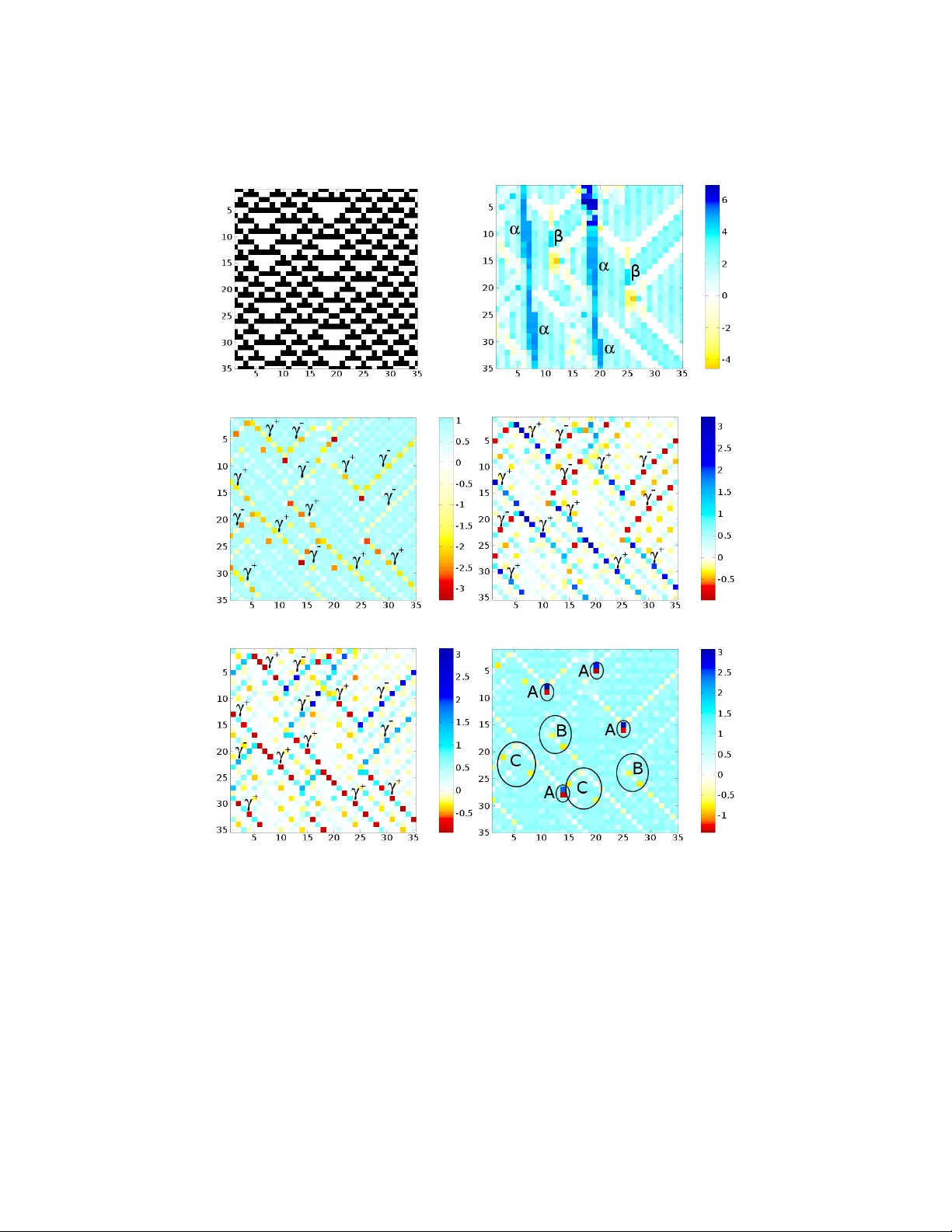
1 A framework f or the local inf ormation dynamics of distrib uted computation in complex systems Joseph T . Lizier 1 , 2 , Mikhail Prokopenko 1 and Albert Y . Zomaya 2 1 CSIR O Computational Informatics, Locked Bag 17, North Ryde, NSW 1670, Australia 2 School of Information T echnologies, The Uni versity of Sydney , NSW 2006, Australia Summary . The nature of distributed computation has often been described in terms of the com- ponent operations of univ ersal computation: information stora ge , transfer and modiﬁcation . W e revie w the ﬁrst complete frame work that quantiﬁes each of these individual information dy- namics on a local scale within a system, and describes the manner in which they interact to create non-trivial computation where “the whole is greater than the sum of the parts”. W e de- scribe the application of the framework to cellular automata, a simple yet powerful model of distributed computation. This is an important application, because the framework is the ﬁrst to provide quantitati ve e vidence for se veral important conjectures about distributed computation in cellular automata: that blinkers embody information storage, particles are information transfer agents, and particle collisions are information modiﬁcation e vents. The framework is also shown to contrast the computations conducted by sev eral well-known cellular automata, highlighting the importance of information coherence in complex computation. The results reviewed here provide important quantitativ e insights into the fundamental nature of distributed computation and the dynamics of comple x systems, as well as impetus for the framew ork to be applied to the analysis and design of other systems. 1.1 Introduction The nature of distrib uted computation has long been a topic of interest in complex sys- tems science, physics, artiﬁcial life and bioinformatics. In particular, emergent com- plex behavior has often been described from the perspectiv e of computation within the system (Mitchell 1998b,a) and has been postulated to be associated with the capability to support univ ersal computation (Langton 1990; W olfram 1984c; Casti 1991). In all of these relev ant ﬁelds, distributed computation is generally discussed in terms of “memory”, “communication”, and “processing”. Memory refers to the stor- age of information by some v ariable to be used in the future of its time-series process. It has been in vestigated in coordinated motion in modular robots (Prokopenko et al. 2006), in the dynamics of inter-e vent distribution times (Goh and Barab ´ asi 2008), and in synchronization between coupled systems (Morgado et al. 2007). Communication 2 Joseph T . Lizier, Mikhail Prokopenk o and Albert Y . Zomaya refers to the transfer of information between one v ariable’ s time-series process and another; it has been shown to be of rele vance in neuroscience (W ibral et al. 2011; Lindner et al. 2011; Marinazzo et al. 2012) and in other biological systems (e.g. dipole- dipole interaction in microtubules (Brown and T uszynski 1999), and in signal trans- duction by calcium ions (Pahle et al. 2008)), social animals (e.g. schooling behavior in ﬁsh (Couzin et al. 2006)), agent-based systems (e.g. the inﬂuence of agents over their en vironments (Klyubin et al. 2005), and in inducing emergent neural structure (Lungarella and Sporns 2006)). Processing refers to the combination of stored and/or transmitted information into a new form; it has been discussed in particular for bio- logical neural networks and models thereof (Kinouchi and Copelli 2006; Atick 1992; S ´ anchez-Monta ˜ n ´ es and Corbacho 2002; Y amada and Aihara 1994) (where it has been suggested as a potential biological driver), and also regarding collision-based comput- ing (e.g. (Jakubowski et al. 1997; Adamatzky 2002), and including soliton dynamics and collisions (Edmundson and Enns 1993)). Signiﬁcantly , these terms correspond to the component operations of T uring uni- versal computation: information storage , inf ormation transfer (or transmission) and information modiﬁcation . Y et despite the obvious importance of these information dynamics , until recently there was no framework for either quantifying them individ- ually or understanding how the y interact to giv e rise to distributed computation. Here, we revie w the ﬁrst complete framew ork (Lizier et al. 2007, 2008c, 2012c, 2010, 2012b; Lizier and Prok openko 2010; Lizier 2013) which quantiﬁes each of these information dynamics or component operations of computation within a system, and describes how they inter-relate to produce distributed computation. W e refer to the dynamics of information for two key reasons here. First, this approach describes the composition of information in the dynamic state update for the time-series process of each v ariable within the system, in terms of ho w information is stored, transferred and modiﬁed. This perspectiv e of state updates brings an important connection between information theory and dynamical systems. Second, the approach focuses on the dy- namics of these operations on information on a local scale in space and time within the system. This focus on the local scale is an important one. Sev eral authors have suggested that a complex system is better characterized by studies of its local dynam- ics than by averaged or overall measures (Shalizi et al. 2006; Hanson and Crutch- ﬁeld 1992), and indeed here we believe that quantifying and understanding distributed computation will necessitate studying the information dynamics and their interplay on a local scale in space and time. Additionally , we suggest that the quantiﬁcation of the indi vidual information dynamics of computation provides three axes of complex- ity within which to in vestigate and classify complex systems, allowing deeper insights into the variety of computation taking place in dif ferent systems. An important focus for discussions on the nature of distributed computation hav e been cellular automata (CAs) as model systems offering a range of dynamical behav- ior , including supporting complex computations and the ability to model complex sys- tems in nature (Mitchell 1998b). W e revie w the application of this framework to CAs here because there is very clear qualitative observation of emergent structures repre- senting information storage, transfer and modiﬁcation therein (Langton 1990; Mitchell 1998b). CAs are a critical proving ground for any theory on the nature of distrib uted 1 A framework for local information dynamics 3 computation: signiﬁcantly , V on Neumann was kno wn to be a strong believer that “a general theory of computation in ‘complex networks of automata’ such as cellular automata would be essential both for understanding complex systems in nature and for designing artiﬁcial complex systems” (Mitchell (1998b) describing V on Neumann (1966)). Information theory provides the logical platform for our in vestigation, and we be- gin with a summary of the main information-theoretic concepts required. W e provide additional background on the qualitativ e nature of distributed computation in CAs, highlighting the opportunity which existed for our framew ork to provide quantitativ e insights. Subsequently , we consider each component operation of universal computa- tion in turn, and describe how to quantify it locally in a spatiotemporal system. As an application, we revie w the measurement of each of these information dynamics at ev ery point in space-time in sev eral important CAs. W e sho w that our framework pro- vided the ﬁrst complete quantitativ e e vidence for a well-known set of conjectures on the emergent structures dominating distrib uted computation in CAs: that blinkers pro- vide information storage, particles provide information transfer, and particle collisions facilitate information modiﬁcation. Furthermore, we describe the manner in which our results implied that the coherence of information may be a deﬁning feature of complex distributed computation. Our ﬁndings are signiﬁcant because these emergent structures of computation in CAs hav e known analogues in many physical systems (e.g. solitons and biological pattern formation processes, coherent wa ves of motion in ﬂocks), and as such this work will contribute to our fundamental understanding of the nature of distributed computation and the dynamics of complex systems. W e ﬁnish by brieﬂy revie wing the subsequent application of the framework to various complex systems, including in analyzing ﬂocking behavior and in a computational neuroscience setting. 1.2 Information-theor etic preliminaries Information theory (Shannon 1948; Cover and Thomas 1991; MacKay 2003) is an obvious tool for quantifying the information dynamics in volved in distributed com- putation. In fact, information theory has already prov en to be a useful framework for the design and analysis of comple x self-org anized systems (e.g. see (Prok openko et al. 2009)). W e begin by re viewing several necessary information theoretic quantities, includ- ing sev eral measures explicitly deﬁned for use with time-series processes. W e also describe local information-theoretic quantities - i.e. the manner in which information- theoretic measures can be used to describe the information content associated with single observations. 1.2.1 Fundamental quantities The fundamental quantity is the Shannon entropy , which represents the uncertainty associated with any measurement x of a random variable X (using units in bits): 4 Joseph T . Lizier, Mikhail Prokopenk o and Albert Y . Zomaya H X = − X x p ( x ) log 2 p ( x ) . (1.1) The joint entropy of two (or more) random variables X and Y is a generalization to quantify the uncertainty of the joint distribution of X and Y : H X,Y = − X x,y p ( x, y ) log 2 p ( x, y ) . (1.2) The conditional entropy of X given Y is the average uncertainty that remains about x when y is known: H X | Y = − X x,y p ( x, y ) log 2 p ( x | y ) . (1.3) The mutual inf ormation (MI) between X and Y measures the average reduction in uncertainty about x that results from learning the value of y , or vice v ersa: I X ; Y = X x,y p ( x, y ) log 2 p ( x, y ) p ( x ) p ( y ) . (1.4) I X ; Y = H X − H X | Y = H Y − H Y | X . (1.5) One can also describe the MI as measuring the information contained in X about Y (or vice versa). The conditional mutual inf ormation between X and Y giv en Z is the mutual in- formation between X and Y when Z is known: I X ; Y | Z = H X | Z − H X | Y ,Z (1.6) = H Y | Z − H Y | X,Z . (1.7) Importantly , the conditional MI I X ; Y | Z can be larger or smaller than the unconditioned I X ; Y (MacKay 2003); it is reduced by redundant information held by Y and Z about X , and increased by syner gy between Y and Z about X (e.g. where X is the result of an exclusi ve-OR or XOR operation between Y and Z ). 1.2.2 Measures f or time-series processes Next, we describe sev eral measures which are explicitly deﬁned for time-series pro- cesses X . The entropy rate is the limiting value of the rate of change of the joint entropy ov er k consecuti ve v alues of a time-series process X , (i.e. measurements x ( k ) n = { x n − k +1 , . . . , x n − 1 , x n } , up to and including time step n , of the random variable X ( k ) n = { X n − k +1 , . . . , X n − 1 , X n } ), as k increases (Co ver and Thomas 1991; Crutch- ﬁeld and Feldman 2003): H µX = lim k →∞ H X ( k ) n k = lim k →∞ H 0 µX ( k ) , (1.8) H 0 µX ( k ) = H X ( k ) n k , (1.9) 1 A framework for local information dynamics 5 where the limit exists. Note that X ( k ) n is a k -dimensional embedding vector of the state of X (T akens 1981). A related deﬁnition is giv en by the limiting value of the conditional entropy of the next value of X (i.e. measurements x n +1 of the random variable X n +1 ) giv en knowledge of the previous k values of X (i.e. measurements x ( k ) n of the random variable X ( k ) n ): H µX = lim k →∞ H X n +1 | X ( k ) n = lim k →∞ H µX ( k ) , (1.10) H µX ( k ) = H X ( k +1) n +1 − H X ( k ) n , (1.11) again, where the limit exists. This can also be viewed as the uncertainty of the next state x ( k ) n +1 giv en the pre vious state x ( k ) n , since x n +1 is the only non-overlapping quantity in x ( k ) n +1 which is capable of carrying any conditional entropy . Cov er and Thomas (1991) point out that these two quantities correspond to two subtly different notions. These authors go on to demonstrate that for stationary processes X , the limits for the two quantities H 0 µ ( X ) and H µ ( X ) exist (i.e. the average entropy rate con verges) and are equal. For our purposes in considering information dynamics, we are interested in the latter formulation H µ ( X ) , since it e xplicitly describes how one random v ariable X n +1 is related to the previous instances X ( k ) n . Grassberger (1986b) ﬁrst noticed that a slow approach of the entropy rate to its limiting value was a sign of complexity . Formally , Crutchﬁeld and Feldman (2003) use the conditional entropy form of the entropy rate (1.10) 1 to observ e that at a ﬁnite block size k , the difference H µX ( k ) − H µX represents the information carrying capacity in size k -blocks that is due to correlations. The sum over all k gives the total amount of structure in the system, quantiﬁed as the effective measure complexity or excess entropy (measured in bits): E X = ∞ X k =0 [ H µX ( k ) − H µX ] . (1.12) The excess entropy can also be formulated as the mutual information between the semi-inﬁnite past and semi-inﬁnite future of the system: E X = lim k →∞ I X ( k ) n ; X ( k + ) n +1 , (1.13) where X ( k + ) n +1 = { X n +1 , X n +2 , . . . , X n + k } is the random variable (with measure- ments x ( k + ) n +1 = { x n +1 , x n +2 , . . . , x n + k } ) referring to the k future values of the pro- cess X (from time step n + 1 onwards). This interpretation is kno wn as the predictive information (Bialek et al. 2001), as it highlights that the excess entropy captures the information in a process’ past which is relev ant to predicting its future. 1.2.3 Local information-theor etic measures Finally , we note that the aforementioned information-theoretic quantities are aver ages ov er all of the observations used to compute the rele vant probability distrib ution func- 1 H µX ( k ) here is equiv alent to h µ ( k + 1) in (Crutchﬁeld and Feldman 2003). 6 Joseph T . Lizier, Mikhail Prokopenk o and Albert Y . Zomaya tions (PDFs). One can also write do wn local or pointwise measures for each of these quantities, representing their v alue for one speciﬁc observation or conﬁguration of the variables ( x, y , z ) being observed. The a verage of a local quantity o ver all observ ations is of course the relev ant av erage information-theoretic measure. Primarily , the Shannon inf ormation content or local entr opy of an outcome x of measurement of the variable X is (MacKay 2003): h ( x ) = − log 2 p ( x ) . (1.14) Note that by con vention we use lo wer-case symbols to denote local information- theoretic measures throughout this chapter . The quantity h ( x ) is simply the informa- tion content attributed to the speciﬁc symbol x , or the information required to predict or uniquely specify that value. Less probable outcomes x hav e higher information con- tent than more probable outcomes, and we have h ( x ) ≥ 0 . Speciﬁcally , the Shannon information content of a given symbol x is the code-length for that symbol in an op- timal encoding scheme for the measurements X , i.e. one that produces the minimal expected code length. 2 Now , note that although the PDF p ( x ) is evaluated for h ( x ) locally at the giv en observation x , it is deﬁned using all of the av ailable (non-local) observations of the variable X which w ould go into ev aluation of the corresponding H ( X ) . That is to say , we deﬁne a certain PDF p ( x ) from all given measurements of a variable X : we can measure local entropies h ( x ) by ev aluating p ( x ) for a giv en observation x , or we can measure av erage entropies H ( X ) from the whole function p ( x ) , and indeed we have H ( X ) = h h ( x ) i when the expectation v alue is taken over p ( x ) . Similarly , we have the local conditional entropy h ( x | y ) = − log 2 p ( x | y ) with H ( X | Y ) = h h ( x | y ) i . Next, the local mutual information (Fano 1961) for a speciﬁc observation ( x, y ) is the information held in common between the speciﬁc values x and y : i ( x ; y ) = h ( x ) − h ( x | y ) , (1.15) = log 2 p ( x | y ) p ( x ) . (1.16) The local mutual information is the difference in code lengths between coding the value x in isolation (under the optimal encoding scheme for X ), or coding the v alue x giv en y (under the optimal encoding scheme for X giv en Y ). Similarly , we hav e the local conditional mutual information : i ( x ; y | z ) = h ( x | z ) − h ( x | y , z ) , (1.17) = log 2 p ( x | y , z ) p ( x | z ) . (1.18) 2 This “optimal code-length” may specify non-integer choices; full discussion of the impli- cations here, practical issues in selecting integer code-lengths, and block-coding optimisations are contained in (Cov er and Thomas 1991, Chapter 5). 1 A framework for local information dynamics 7 Indeed, the form of i ( x ; y ) and i ( x ; y | z ) are derived directly from four postulates by Fano (1961, ch. 2): once-differentiability , similar form for conditional MI, additi vity (i.e. i ( { y n , z n } ; x n ) = i ( y n ; x n ) + i ( z n ; x n | y n ) ), and separation for independent ensembles. This deriv ation means that i ( x ; y ) and i ( x ; y | z ) are uniquely speciﬁed, up to the base of the logarithm. Of course, we ha ve I ( X ; Y ) = h i ( x ; y ) i and I ( X ; Y | Z ) = h i ( x ; y | z ) i , and like I ( X ; Y ) and I ( X ; Y | Z ) , the local values are symmetric in x and y . Importantly , i ( x ; y ) may be positiv e or negati ve, meaning that one variable can either positiv ely inform us or actually misinform us about the other . An observer is misinformed where, conditioned on the value of y the observed outcome of x was r elatively unlikely as compared to the unconditioned probability of that outcome (i.e. p ( x | y ) < p ( x ) ). Similarly , i ( x ; y | z ) can become neg ative where p ( x | y , z ) < p ( x | z ) . Applied to time-series data, local measures tell us about the dynamics of informa- tion in the system, since they vary with the speciﬁc observations in time, and local val- ues are kno wn to re veal more details about the system than the a verages alone (Shalizi 2001; Shalizi et al. 2006). 1.3 Cellular automata 1.3.1 Introduction to Cellular A utomata Cellular automata (CA) are discrete dynamical systems consisting of an array of cells which each synchronously update their discrete v alue as a function of the values of a ﬁxed number of spatially neighboring cells using a uniform rule. Although the behavior of each individual cell is very simple, the (non-linear) interactions between all cells can lead to v ery intricate global behavior , meaning CAs ha ve become a classic e xample of self-organized complex behavior . Of particular importance, CAs have been used to model real-world spatial dynamical processes, including ﬂuid ﬂow , earthquakes and biological pattern formation (Mitchell 1998b). The neighborhood of a cell used as inputs to its update rule at each time step is usually some regular conﬁguration. In 1D CAs, this means the same range r of cells on each side and including the current value of the updating cell. One of the simplest variety of CAs – 1D CAs using binary values, deterministic rules and one neighbor on either side ( r = 1 ) – are known as the Elementary CAs , or ECAs . Example ev olutions of ECAs from random initial conditions may be seen in Fig. 1.2a and Fig. 1.6a. For more complete deﬁnitions of CAs, including the deﬁnition of the W olfram rule number con vention for specifying update rules, see W olfram (2002). W olfram (1984c, 2002) sought to classify the asymptotic behavior of CA rules into four classes: I. Homogeneous state; II. Simple stable or periodic structures; III. Chaotic aperiodic behavior; and IV . Complicated localized structures, some propagating. Much conjecture remains as to whether these classes are quantitativ ely distinguishable, e.g. see Gray (2003), howe ver they do provide an interesting analogy (for discrete-state and time) to our knowledge of dynamical systems, with classes I and II representing 8 Joseph T . Lizier, Mikhail Prokopenk o and Albert Y . Zomaya ordered behavior , class III representing chaotic behavior , and class IV representing complex beha vior and considered as lying between the ordered and chaotic classes. More importantly though, the approach seeks to characterize complex behavior in terms of emergent structure in CAs, reg arding gliders , particles and domains . Quali- tativ ely , a domain may described as a set of background conﬁgurations in a CA, for which any given conﬁguration will update to another such conﬁguration in the set in the absence of any disturbance. Domains are formally deﬁned within the framew ork of computational mechanics (Hanson and Crutchﬁeld 1992) as spatial process languages in the CA. Particles are qualitativ ely considered to be moving elements of coherent spatiotemporal structure. Gliders are particles which repeat periodically in time while moving spatially (repetitive non-moving structures are known as blinkers ). Formally , particles are deﬁned within the framework of computational mechanics as a boundary between two domains (Hanson and Crutchﬁeld 1992); as such, they can also be termed as domain walls, though this is typically used with reference to aperiodic particles. These emer gent structures are more clearly visible when the CA is ﬁltered in some way . Early ﬁltering methods were hand-crafted for speciﬁc CAs (relying on the user knowing the pattern of background domains) (Grassberger 1983, 1989), while later methods can be automatically applied to any giv en CA. These include:  -machines (Hanson and Crutchﬁeld 1992), input entropy (W uensche 1999), local information (Helvik et al. 2004), and local statistical complexity (Shalizi et al. 2006). All of these ﬁltering techniques produce a single ﬁltered view of the structures in the CA: our measures of local information dynamics will present sev eral ﬁltered views of the dis- tributed computation in a CA, separating each operation on information. The ECA examples analyzed in this chapter are introduced in Section 1.3.3. 1.3.2 Computation in Cellular A utomata CAs can be interpreted as undertaking distributed computation: it is clear that “data represented by initial conﬁgurations is processed by time ev olution” (W olfram 1984c). As such, computation in CAs has been a popular topic for study (see Mitchell (1998b)), with a particular focus in observing or constructing (T uring) universal computation in certain CAs. An ability for universal computation is deﬁned to be where “suitable ini- tial conﬁgurations can specify arbitrary algorithm procedures” in the computing entity , which is capable of “ev aluating any (computable) function” (W olfram 1984c). W ol- fram (1984c,a) conjectured that all class IV complex CAs were capable of univ ersal computation. He went on to state that prediction in systems exhibiting univ ersal com- putation is limited to explicit simulation of the system, as opposed to the av ailability of any simple formula or “short-cut”, drawing parallels to the halting problem for uni- versal Turing machines (W olfram 1984c,a) which are echoed by Langton (1990) and Casti (1991). (Casti extended the analogy to undecidable statements in formal systems, i.e. G ¨ odel’ s Theorem). The capability for universal computation has been proven for sev eral CA rules, through the design of rules generating elements to (or by identifying elements which) speciﬁcally provide the component operations required for universal computation: information storage, transmission and modiﬁcation. Examples here in- 1 A framework for local information dynamics 9 clude most notably the Game of Life (Conway 1982) and ECA rule 110 (Cook 2004); also see Lindgren and Nordahl (1990) and discussions by Mitchell (1998b). The focus on elements providing information storage, transmission and modiﬁca- tion pervades discussion of all types of computation in CAs, e.g. (Adamatzky 2002; Jakubowski et al. 2001). W olfram (1984a) claimed that in class III CAs information propagates over an inﬁnite distance at a (regular) ﬁnite speed, while in class IV CAs information propagates at an irregular speed over an inﬁnite range. Langton (1990) hypothesized that complex behavior in CAs exhibited the three component operations required for universal computation. He suggested that the more chaotic a system be- comes the more information transmission increases, and the more ordered a system becomes the more information it stores. Complex behavior was said to occur at a phase transition between these extremes requiring an intermediate lev el of both information storage and transmission: if information propagates too well, coherent information de- cays into noise . Langton elaborates that transmission of information means that the “dynamics must provide for the propagation of information in the form of signals ov er arbitrarily long distances”, and suggests that particles in CAs form the basis of these signals. T o complete the qualitati ve identiﬁcation of the elements of computation in CAs, he also suggested that blinkers formed the basis of information storage, and collisions between propagating (particles) and static structures (blinkers) “can mod- ify either stored or transmitted information in the support of an overall computation”. Rudimentary attempts were made at quantifying the av erage information transfer (and to some extent information storage), via mutual information (although as discussed later this is a symmetric measure not capturing directional transfer). Recognizing the importance of the emergent structures to computation, sev eral examples exist of at- tempts to automatically identify CA rules which giv e rise to particles and gliders, e.g. (W uensche 1999; Eppstein 2002), suggesting these to be the most interesting and com- plex CA rules. Sev eral authors howe ver criticize the aforementioned approaches of attempting to classify CAs in terms of their generic behavior or “b ulk statistical properties”, suggest- ing that the wide range of dif fering dynamics taking place across the CA makes this problematic (Hanson and Crutchﬁeld 1992; Mitchell 1998b). Gray (2003) suggests that there there may indeed be classes of CAs capable of more complex computation than univ ersal computation alone. More importantly , Hanson and Crutchﬁeld (1992) criticize the focus on universal computational ability as drawing away from the abil- ity to identify “generic computational properties”, i.e. a lack of ability for univ ersal computation does not mean a CA is not undertaking any computation at all. Alter- nativ ely , these studies suggest that analyzing the rich space-time dynamics within the CA is a more appropriate focus. As such, these and other studies have analyzed the local dynamics of intrinsic or other speciﬁc computation, focusing on particles facili- tating the transfer of information and collisions facilitating the information processing. Notew orthy examples here include: the method of applying ﬁlters from the domain of computational mechanics by Hanson and Crutchﬁeld (1992); and analysis using such computational mechanics ﬁlters of CA rules selected via ev olutionary computation to perform classiﬁcation tasks by Mitchell et al. (1994, 1996). Related are studies which deeply inv estigate the nature of particles and their interactions, e.g. particle types and 10 Joseph T . Lizier, Mikhail Prokopenk o and Albert Y . Zomaya their interaction products identiﬁed for particular CAs (Mitchell et al. 1996; Boccara et al. 1991; Martinez et al. 2006), and rules established for their interaction products by Hordijk et al. (2001). Despite such interest, until recently there was no complete framework that locally quantiﬁes the indi vidual information dynamics of distributed computation within CAs or other systems. In this revie w , we describe how the information dynamics can be locally quantiﬁed within the spatiotemporal structure of a CA. In particular, we de- scribe the dynamics of how information storage and information transfer interact to giv e rise to information processing. Our approach is not to quantify computation or ov erall complexity , nor to identify univ ersal computation or determine what is being computed; it is simply intended to quantify the component operations in space-time. 1.3.3 Examples of distributed computation in CAs In this chapter, we revie w analysis of the computation carried out by se veral important ECA rules: • Class IV complex rules 110 and 54 (W olfram 2002) (see Fig. 1.4a and Fig. 1.2a), both of which exhibit a number of glider types and collisions. ECA rule 110 is the only prov en computationally universal ECA rule (Cook 2004). • Rules 22 and 30 as representativ e class III chaotic rules (W olfram 2002) (see rule 22 in Fig. 1.6a); • Rules 18 as a class III rule which contains domain walls against a chaotic back- ground domain (W olfram 1984b; Hanson and Crutchﬁeld 1992). These CAs each carry out an intrinsic computation of the e volution to their ultimate attractor and phase on it (see W uensche (1999) for a discussion of attractors and state space in ﬁnite-sized CAs). That is to say , we view the attractor as the end point of an intrinsic computation by the CA – the dynamics of the transient to the attractor may contain information storage, transfer and modiﬁcation, whi le the dynamics on the attractor itself can only contain information storage (since the attractor is either a ﬁxed point or periodic process here). As such, we are generally only interested in studying computation during the transient dynamics here, as non-trivial computation processes. W e also examine a CA carrying out a “human-understandable” computational task. Rule φ par is a 1D CA with range r = 3 (the 128-bit W olfram rule number 0xfeed- ffdec1aaeec0eef000a0e1a020a0) that was ev olved by Mitchell et al. (1994, 1996) to classify whether the initial CA conﬁguration had a majority of 1’ s or 0’ s by reaching a ﬁxed-point conﬁguration of all 1’ s for the former or all 0’ s for the latter . This CA rule achieved a success rate abov e 70% in its task. An example e volution of this CA can be seen in Fig. 1.5a. The CA appears to carry out this computation using blink- ers and domains for information storage, gliders for information transfer and glider collisions for information modiﬁcation. The CA exhibits an initial emergence of do- main regions of all 1’ s or all 0’ s storing information about local high densities of either value. Where these domains meet, a checkerboard domain propagates slowly (1 cell per time step) in both directions, transferring information of a soft uncertainty in this part of the CA. Some “certainty” is provided where the glider of the leading edge of 1 A framework for local information dynamics 11 a checkerboard encounters a blinker boundary between 0 and 1 domains, which stores information about a hard uncertainty in that region of the CA. This results in an in- formation modiﬁcation ev ent where the domain on the opposite side of the blinker to the incoming checkerboard is concluded to represent the higher density state, and is allowed to propagate over the checkerboard. This new information transfer associ- ated with local decision of which is the higher density state has evolv ed to occur at a faster speed (3 cells per time step) than the checkerboard uncertainty; it can overrun checkerboard regions, and in fact collisions of opposing types of this strong propaga- tion give rise to the (hard uncertainty) blinker boundaries in the ﬁrst place. The ﬁnal conﬁguration is therefore the result of this distributed computation. Quantiﬁcation of the local information dynamics via these three axes of complexity (information storage, transfer and modiﬁcation) will provide quite detailed insights into the distributed computation carried out in a system. In all of these CAs we e xpect local measures of information storage to highlight blinkers and domain regions, local measures of information transfer to highlight particles (including gliders and domain walls), and local measures of information modiﬁcation to highlight particle collisions. This will provide a deeper understanding of computation than single or generic measures of bulk statistical behavior , from which conﬂict often arises in attempts to provide classiﬁcation of complex behavior . In particular , we seek clariﬁcation on the long-standing debate regarding the nature of computation in ECA rule 22. Suggestions that rule 22 is complex include the dif ﬁculty in estimating the metric entropy (i.e. tem- poral entropy rate) for rule 22 by Grassberger (1986b), due to “complex long-range effects, similar to a critical phenomenon” (Grassberger 1986a). This effecti vely cor- responds to an implication that rule 22 contains an inﬁnite amount of memory (see Section 1.4.1). Also, from an initial condition of only a single “on” cell, rule 22 forms a pattern known as the “Sierpinski Gasket” (W olfram 2002) which exhibits clear frac- tal structure. Furthermore, rule 22 is a 1D mapping of the 2D Game of Life CA (kno wn to have the capability for uni versal computation (Conway 1982)) and in this sense is referred to as “life in one dimension” (McIntosh 1990), and complex structure in the language generated by iterations of rule 22 has been identiﬁed by Badii and Politi (1997). Also, we reported in (Lizier et al. 2012b) that we hav e in vestigated the C 1 complexity measure (Lafusa and Bossomaier 2005) (an enhanced version of the vari- ance of the input entropy (W uensche 1999)) for all ECAs, and found rule 22 to clearly exhibit the largest value of this measure (0.78 bits to rule 110’ s 0.085 bits). On the other hand, suggestions that rule 22 is not complex include its high sensiti vity to ini- tial conditions leading to W olfram (2002) classifying it as class III chaotic. Gutowitz and Domain (1997) claim this renders it as chaotic despite the subtle long-range ef- fects it displays, further identifying its fast statistical con ver gence, and exponentially long and thin transients in state space (see W uensche (1999)). Importantly , no coherent structure (particles, collisions, etc.) is found for typical proﬁles of rule 22 using a num- ber of known ﬁlters for such structure (e.g. local statistical complexity (Shalizi et al. 2006)): this reﬂects the paradigm shift to an e xamination of local dynamics rather than generic, overall or averaged analysis. In our approach, we seek to combine this local viewpoint of the dynamics with a quantitativ e breakdown of the individual elements of computation, and we will revie w the application to rule 22 in this light. 12 Joseph T . Lizier, Mikhail Prokopenk o and Albert Y . Zomaya 1.4 Information Storage In this section we revie w the methods to quantify information storage on a local scale in space and time, as presented in (Lizier et al. 2012c). W e describe how total infor- mation storage used in the future is captured by excess entropy , and introduce activ e information storage to capture the amount of information storage that is currently in use. W e revie w the application of local proﬁles of both measures to cellular automata. 1.4.1 Excess entropy as total inf ormation storage Although discussion of information storage or memory in CAs has often focused on periodic structures (particularly in construction of univ ersal T uring machines), infor - mation storage does not necessarily entail periodicity . The excess entropy Eq. (1.12, 1.13) more broadly encompasses all types of structure and memory by capturing correlations across all lengths of time, including non-linear correlations. It is quite clear from the predictiv e information formulation of the excess entropy Eq. (1.13) – as the informa- tion from a process’ past that is contained its future – that it is a measure of the total information storage used in the future of a system. 3 W e use the term univariate excess entr opy 4 to refer to measuring the excess en- tropy for indi vidual variables X using their one-dimensional time-series process, i.e. E X = lim k →∞ I X ( k ) n ; X ( k + ) n +1 from Eq. (1.13). This is a measure of the averag e memory for each variable X . Furthermore, we use the term collective excess en- tr opy to refer to measuring the temporal excess entropy for a collective of variables X = { X 1 , X 2 , . . . , X m } (e.g. a set of neighboring cells in a CA) using their two- dimensional time-series process. Considered as the mutual information between their joint past and future, i.e. a joint temporal predictiv e information: E X = lim k →∞ I { X ( k ) 1 ,n , X ( k ) 2 ,n ,..., X ( k ) m,n } ; { X ( k + ) 1 ,n +1 , X ( k + ) 2 ,n +1 ,..., X ( k + ) m,n +1 } , (1.19) this is a measure of the avera ge total memory stored in the collective (i.e. stored collec- tively by a set of cells in a CA). Collecti ve excess entropy could be used for example to quantify the “undiscov ered collective memory that may present in certain ﬁsh schools” (Couzin et al. 2006). Grassberger (1986b,a) studied temporal entropy rate estimates for several ECAs in order to gain insights into their excess entropies. He rev ealed div ergent collectiv e excess entropy for a number of rules, including rule 22, implying a highly complex process. This case has been described by Lindgren and Nordahl (1988) as “a phe- nomenon which can occur in more complex en vironments”, as with strong long-range 3 In (Lizier et al. 2012c) we provide further comment on the relation to the statistical com- plexity (Crutchﬁeld and Y oung 1989), which measures all information stored by the system which may be used in the future, while the excess entr opy measures that information which is used by the system at some point in the future. The relation between the two concepts is cov ered in a more general mathematical context by Shalizi and Crutchﬁeld (2001). 4 Called “single-agent excess entropy” in (Lizier et al. 2012c). 1 A framework for local information dynamics 13 correlations a semi-inﬁnite sequence “could store an inﬁnite amount of information about its continuation” (as per the predictiv e information form of the excess entropy Eq. (1.13)). On the other hand, inﬁnite collective excess entropy can also be achiev ed for systems that only tri vially utilise all of their available memory (e.g. simply copying cell values to the right when started from random initial states). Rule 22 w as inferred to hav e H µ,N = 0 and inﬁnite collective e xcess entropy , which was interpreted as a pro- cess requiring an inﬁnite amount of memory to maintain an aperiodicity (Crutchﬁeld and Feldman 2003). In attempting to quantify local information dynamics of distributed computation here, our focus is on information storage for single variables or cells rather than the joint information storage across the collectiv e. W ere the univ ariate excess entropy found to be div ergent (this has not been demonstrated), this may be more signiﬁcant than for the collecti ve case: di vergent collecti ve e xcess entropy implies that the collec- tiv e is at least trivially utilizing all of its av ailable memory (and even the chaotic rule 30 exhibits this), whereas div ergent univ ariate excess entropy implies that all cells are individually highly utilizing the resources of the collectiv e in a highly complex pro- cess. Again though, we emphasize that our focus is on local measures in time as well as space, which we present in the next section. First we note that with respect to CAs, where each cell has only a ﬁnite number of values b and takes direct inﬂuence from only its single past value and the values of a ﬁnite number of neighbors, the meaning of (either average or local) information storage being greater log 2 b bits (let alone inﬁnite) in the time series process of a single cell is not immediately ob vious. Clearly , a cell in an ECA cannot store more than 1 bit of information in isolation. Ho wever , the bidir ectional communication in CAs effec- tiv ely allo ws a cell to store e xtra information in neighbors (e ven be yond the immediate neighbors), and to subsequently retrieve that information from those neighbors at a later point in time. While measurement of the excess entropy does not explicitly look for such self-inﬂuence communicated through neighbors, it is indeed the method by which a signiﬁcant portion of information is channeled. Considering the predictive information interpretation in Eq. (1.13), it is easy to picture self-inﬂuence between semi-inﬁnite past and future blocks being conv eyed via neighbors (see Fig. 1.1a). This is akin to the use of stigmergy (indirect communication through the en vironment, e.g. see Klyubin et al. (2004)) to communicate with oneself. A measurement of more than log 2 b bits stored by a cell on average, or indeed an inﬁnite information storage, is then a perfectly v alid result: in an inﬁnite CA, each cell has access to an inﬁnite amount of neighbors in which to store information which can later be used to inﬂuence its own future. Note howe ver , that since the storage medium is shared by all cells, one should not think about the total memory as the total number of cells multiplied by this average. The total memory would be properly measured by the collectiv e excess entropy , which takes into account the inherent redundancy here. Follo wing similar reasoning (i.e. that information may be stored and retriev ed from one’ s neighbors), we note that a v ariable can store information reg ardless of whether it is causally connected with itself. Also, note that a variable can be perceived to store in- formation simply as a result of ho w that v ariable is dri ven (Obst et al. 2013), i.e. where information is physically stored elsewhere in the system b ut recurs in the v ariable at 14 Joseph T . Lizier, Mikhail Prokopenk o and Albert Y . Zomaya (a) Excess Entropy (b) Activ e Information Storage Fig. 1.1: Measures of information storage in the time-series processes of single vari- ables in distributed systems. (a) Excess Entropy: total information from the variable’ s past that is predictive of its future. (b) Active Information storage: the information storage that is curr ently in use in determining the next v alue of the variable. The stored information can be conv eyed directly through the variable itself or via feed- back from neighbors. (NB: This ﬁgure is reprinted from (Lizier et al. 2012c), Lizier , J. T ., Prokopenko, M., and Zomaya, A. Y ., Local measures of information storage in complex distributed computation, Information Sciences , 208:39–54, Copyright (2012), with permission from Elsevier .) different time steps (e.g. see the description of information storage in feed-forward loop motifs in (Lizier et al. 2012a)). 1.4.2 Local excess entropy W e now shift focus to local measures of information storage, which ha ve the potential to pro vide more detailed insights into information storage structures and their in volve- ment in computation than single ensemble measures. The local e xcess entr opy is a measure of how much information a given variable is storing at a particular point in time (Shalizi 2001). 5 The local excess entropy e X ( n + 1) of a process is simply the local mutual information Eq. (1.16) of the semi-inﬁnite past and future of the process X at the giv en time step n + 1 : e X ( n + 1) = lim k →∞ log 2 p ( x ( k ) n , x ( k + ) n +1 ) p ( x ( k ) n ) p ( x ( k + ) n +1 ) . (1.20) Note that the excess entropy is the average of the local v alues, E X = h e X ( n ) i . The limit k → ∞ is an important part of this deﬁnition, since correlations at all time 5 This is as per the original formulation of the local excess entropy by Shalizi (2001), how- ev er this presentation is for a single time-series rather than the light-cone formulation used there. 1 A framework for local information dynamics 15 scales should be included in the computation of information storage. Since this is not computationally feasible in general, we retain the notation e X ( n + 1 , k ) to denote ﬁnite- k estimates of e X ( n + 1) . The notation is generalized for lattice systems (such as CAs) with spatially-or der ed variables to represent the local e xcess entropy for cell X i at time n + 1 as: e ( i, n + 1) = lim k →∞ log 2 p ( x ( k ) i,n , x ( k + ) i,n +1 ) p ( x ( k ) i,n ) p ( x ( k + ) i,n +1 ) . (1.21) Again, e ( i, n + 1 , k ) is used to denote ﬁnite- k estimates of e ( i, n + 1) . Local excess entropy is deﬁned for e very spatiotemporal point ( i, n ) in the system. (Alternativ ely , the collectiv e excess entropy can only be localized in time). As a local mutual information, the local excess entropy may be positive or negativ e, meaning the past history of the cell can either positiv ely inform us or actually misin- form us about its future. An observer is misinformed where a giv en semi-inﬁnite past and future are relativ ely unlik ely to be observed together as compared to the product of their mar ginal probabilities. Another view is that we ha ve misinformati ve values when p ( x ( k + ) i,n +1 | x ( k ) i,n ) < p ( x ( k + ) i,n +1 ) , meaning that taking the past x ( k ) i,n into account reduced the probability of the future which was observed x ( k + ) i,n +1 . 1.4.3 Active inf ormation storage The excess entropy measures the total stored information which will be used at some point in the future of the time-series process of a v ariable, possibly but not necessarily at the next time step n + 1 . In examining the local information dynamics of compu- tation, we are interested in how much of the stored information is actually in use at the next time step. As we will see in Section 1.6, this is particularly important in un- derstanding how stored information interacts with information transfer in information processing. As such, the active information storage A X was introduced in (Lizier et al. 2012c) as the average mutual information between the (semi-inﬁnite) past state of the process and its next value , as opposed to its whole (semi-inﬁnite) future: A X = lim k →∞ I ( X ( k ) n ; X n +1 ) . (1.22) The local active inf ormation storage is then a measure of the amount of information storage in use by the process at a particular time-step n + 1 : a X ( n + 1) = lim k →∞ log 2 p ( x ( k ) n , x n +1 ) p ( x ( k ) n ) p ( x n +1 ) , (1.23) = lim k →∞ log 2 p ( x n +1 | x ( k ) n ) p ( x n +1 ) , (1.24) and we have A X = h a X ( n ) i . W e retain the notation a X ( n + 1 , k ) and A X ( k ) for ﬁnite- k estimates. Ag ain, we generalize the measure for v ariable X i in a lattice system as: 16 Joseph T . Lizier, Mikhail Prokopenk o and Albert Y . Zomaya a ( i, n + 1) = lim k →∞ log 2 p ( x ( k ) i,n , x i,n +1 ) p ( x ( k ) i,n ) p ( x i,n +1 ) , (1.25) and use a ( i, n + 1 , k ) to denote ﬁnite- k estimates there, noting that the local acti ve in- formation storage is deﬁned for ev ery spatiotemporal point ( i, n ) in the lattice system. The av erage activ e information storage will always be positiv e (as for the excess en- tropy), but is bounded abov e by log 2 b bits if the v ariable takes one of b discrete v alues. The local activ e information storage is not bound in this manner howe ver , with values larger than log 2 b indicating that the particular past of an variable provides strong posi- tiv e information about its ne xt v alue. Furthermore, the local activ e information storage can be negati ve, where the past history of the v ariable is actually misinformative about its next value. An observer is misinformed where the past history and observed next value are relativ ely unlikely to occur together as compared to their separate occurrence. 1.4.4 Local information storage r esults In this and subsequent results sections, we revie w the application of these local mea- sures in (Lizier et al. 2007, 2008c, 2012c, 2010, 2012b; Lizier and Prokopenko 2010; Lizier 2013) to sample CA runs. As described earlier, we are interested in studying the non-trivial computation during the transient dynamics before an attractor is reached. Certainly it would be easier to study these information dynamics on attractors – since the dynamics there are cyclo-stationary (because the attractors in ﬁnite-length CAs in- volv e only ﬁxed or periodic dynamics) – howe ver as described in Section 1.3.3 the computation there is trivial. T o in vestigate the dynamics of the transient, we estimate the required probability distribution functions (PDFs) from CA runs of 10 000 cells, initialized from random values, in order to generate a large ensemble of transient au- tomata dynamics. W e retain only a relativ ely short 600 time steps for each cell, in order to av oid attractor dynamics and focus on quasi-stationary transient dynamics during that short time period. Alternatively , for φ par we used 30 000 cells with 200 time steps retained. Periodic boundary conditions were used. Observations taken at ev ery spatiotemporal point in the CA were used in estimating the required PDFs, since the cells in the CA are homogeneous variables and quais-stationarity is assumed ov er the relativ ely short time interval. The results and the ﬁgures displayed here were produced using the open source J ava Information Dynamics T oolkit (Lizier 2012), which can be used in Matlab/Octave and Python as well as Jav a. All results can be reproduced using the Matlab/Octav e script GsoChapterDemo2013.m in the demos/octave/CellularAutomata example distributed with this toolkit. W e make estimates of the measures with ﬁnite values of k , noting that the insights described here could not be attained unless a rea- sonably large value of k was used in order to capture a large proportion of the cor- relations. Determination of an appropriate value of k was discussed in (Lizier et al. 2012c), and in (Lizier et al. 2008c) for the related transfer entropy measure presented in Section 1.5. As a rule of thumb, k should at least be larger than the period of any regular background domain in order to capture the information storage underpinning its continuation. 1 A framework for local information dynamics 17 W e begin by examining the results for rules 54 and 110, which contain regular gliders against periodic background domains. For the CA runs described above, sample areas of the large CAs are shown in Fig. 1.2a and Fig. 1.4a, while the corresponding local proﬁles of e ( i, n, k = 8) generated are displayed in Fig. 1.2b and Fig. 1.4b, and the local proﬁles of a ( i, n, k = 16) in Fig. 1.2c and Fig. 1.4c. It is quite clear that positi ve information storage is concentrated in the v ertical gliders or blink ers, and the domain regions. As expected, these results provide quantitativ e evidence that the blinkers are the dominant information storage entities . That the domain regions contain signiﬁcant information storage should not be surprising, since as a periodic sequence its past does indeed store information about its future. In fact, the local values for each measure form spatially and temporally periodic patterns in the domains, corresponding to the spatial and temporal periodicities e xhib- ited in the underlying raw v alues. Certainly if the dynamics are only composed of a consistent domain pattern (which is deterministic when viewing single cells’ time se- ries), then for a ( i, n, k ) for example we will always hav e p ( x n +1 | x ( k ) n ) = 1 and if p ( x n +1 ) is balanced then a ( i, n, k ) would be constant across the CA. Ho wever , the e x- istence of discontinuities in the domain, e.g. gliders, reduces p ( x n +1 | x ( k ) n ) here, and does so differently for each x ( k ) n conﬁguration in the domain. Imbalances in p ( x n +1 ) can also contribute to differences in storage across the domain. These factors leads to the spatiotemporal periodicities of information storage that are observed in the do- mains. While the local activ e information storage indicates a similar amount of stored information in use to compute each space-time point in both the domain and blinker areas, the local excess entropy rev eals a larger total amount of information is stored in the blinkers. For the blinkers known as α and β in rule 54 (Hordijk et al. 2001) this is because the temporal sequences of the center columns of the blinkers (0-0-0-1, with e ( i, n, k = 8) in the range 5.01 to 5.32 bits) are more complex than those in the domain (0-0-1-1 and 0-1, with e ( i, n, k = 8) in the range 1.94 to 3.22 bits), e ven where they are of the same period. W e have e ( i, n, k = 8) > 1 bit here due to the distributed information storage supported by bidirectional communication (as discussed earlier). Such bidirectional communication is also critical to these periodic domain sequences being longer than two time steps – the maximum period that a binary cell could sustain in isolation (e.g. the period-7 domain in rule 110). Another area of strong information storage appears to be the “wake” of the more complex gliders in rule 110 (see the glider at top right of Fig. 1.4b and Fig. 1.4c). This result aligns well with our observation (Lizier et al. 2008c) that the dynamics following the leading edge of regular gliders consists lar gely of “non-traveling” information. The presence of the information storage is shown by both measures, although the relative strength of the total information storage is again rev ealed only by the local excess entropy . Negati ve v alues of a ( i, n, k = 16) for rules 54 and 110 are also visible in Fig. 1.2c and Fig. 1.4c. Interestingly , negati ve local components of local activ e information storage measure are concentrated in the trav eling glider areas (e.g. γ + and γ − for rule 54 (Hordijk et al. 2001)), providing a good spatiotemporal ﬁlter of these struc- 18 Joseph T . Lizier, Mikhail Prokopenk o and Albert Y . Zomaya (a) Raw CA (b) e ( i, n, k = 8) (c) a ( i, n, k = 16) (d) t ( i, j = 1 , n, k = 16) (e) t ( i, j = − 1 , n, k = 16) (f) s ( i, n, k = 16) Fig. 1.2: Local information dynamics in rule 54 for the raw values in (a) (black for “1”, white for “0”). 35 time steps are displayed for 35 cells, and time increases down the page for all CA plots. All units are in bits. (b) Local excess entropy e ( i, n, k = 8) ; (c) Local active information storage a ( i, n, k = 16) ; Local apparent transfer entropy: (d) one cell to the right t ( i, j = 1 , n, k = 16) , (e) one cell to the left t ( i, j = − 1 , n, k = 16) ; (f) Local separable information s ( i, n, k = 16) . 1 A framework for local information dynamics 19 Fig. 1.3: Close up of raw values of rule 54. “x” and “+” mark some positions in the γ + and γ − gliders respectively . Note their point of coincidence in collision type “ A”, with “ • ” marking the subsequent non-trivial information modiﬁcation as detected us- ing s ( i, n, k = 16) < 0 . (Reprinted with permission from (Lizier et al. 2010) J. T . Lizier , M. Prokopenko, and A. Y . Zomaya, “Information modiﬁcation and particle col- lisions in distributed computation, ” Chaos , vol. 20, no. 3, p. 037109, 2010. Copyright 2010, AIP Publishing LLC.) tures. This is because when a traveling glider is encountered at a gi ven cell, the past history of that cell (being part of the background domain) is misinformativ e about the next value, since the domain sequence was more likely to continue than be interrupted. For example, see the marked positions of the γ gliders in Fig. 1.3. There we hav e p ( x n +1 | x ( k =16) n ) = 0 . 25 and p ( x n +1 ) = 0 . 52 : since the next value occurs relati vely infrequently after the given history , we hav e a misinformativ e a ( n, k = 16) = − 1 . 09 bits. This is juxtaposed with the points four time steps before those marked “x”, which have the same history x ( k =16) n but are part of the domain, with p ( x n +1 | x ( k =16) n ) = 0 . 75 and p ( x n +1 ) = 0 . 48 giving a ( n, k = 16) = 0 . 66 bits, quantifying the positiv e information storage there. Note that the points with mis- informativ e information storage are not necessarily those selected by other ﬁltering techniques as part of the gliders: e.g. the ﬁnite state transducers technique (using left to right scanning by con vention) by Hanson and Crutchﬁeld (1997) would identify points 3 cells to the right of those marked “x” as part of the γ + glider . The local excess entropy produced some negati ve values around trav eling gliders, though these were far less localized on the gliders themselves and less consistent in occurrence than for the local active information storage. This is because the local ex- cess entropy , as measure of total information storage into the future, is more loosely tied to the dynamics at the giv en spatiotemporal point. The effect of a glider encounter on e ( i, n, k ) is smeared out in time, and in fact the dynamics may store more positiv e information in total than the misinformation encountered at the speciﬁc location of the glider . F or example, glider pairs were observed in (Lizier et al. 2012c) to have positive total information storage, since a glider encounter becomes much more likely in the wake of a pre vious glider . 20 Joseph T . Lizier, Mikhail Prokopenk o and Albert Y . Zomaya As another rule containing regular gliders against a periodic background domain, analysis of the raw values of φ par in Fig. 1.5a provides similar results for e ( i, n, k = 5) (not shown, see (Lizier 2013)) and a ( i, n, k = 10) in Fig. 1.5b here. One distinction is that the blinker here contains no more stored information than the domain, since it is no more complicated. Importantly , we conﬁrm the information storage capability of the blinkers and domains in this human understandable computation. Another interesting example is provided by ECA rule 18, which contains domain walls against a seemingly irregular background domain. W e measured the local infor- mation proﬁles for e ( i, n, k = 8) and a ( i, n, k = 16) in (Lizier et al. 2012c) (shown in that paper , but not here). Importantly , the most signiﬁcant negati ve components of the local active information storage are concentrated on the domain walls: analogous to the re gular gliders of rule 54, when a domain wall is encountered the past history of the cell becomes misinformative about its next value. There is also interesting infor- mation storage dynamics in the background domain for rule 18, discussed in detail in (Lizier et al. 2012c). Finally , we examine ECA rule 22, suggested to have inﬁnite collective excess entropy (Grassberger 1986b,a) but without any known coherent structural elements (Shalizi et al. 2006). For the raw values of rule 22 displayed in Fig. 1.6a, the calculated local excess entropy proﬁle is shown in Fig. 1.6b, and the local acti ve information stor- age proﬁle in Fig. 1.6c. While information storage certainly occurs for rule 22, these plots provide evidence that there is no coherent structure to this storage. This is another clear example of the utility of examining local information dynamics over ensemble estimates, giv en the earlier discussion on collectiv e excess entropy for rule 22. In summary , we have demonstrated that the local active information storage and local excess entropy provide insights into information storage dynamics that, while often similar in general, are sometimes subtly different. While both measures provide useful insights, the local activ e information storage is the most useful in a real-time sense, since calculation of the local excess entropy requires knowledge of the dynam- ics an arbitrary distance into the future. 6 Furthermore, it also provides the most specif- ically localized insights, including ﬁltering moving elements of coherent spatiotempo- ral structure. This being said, it is not capable of identifying the information source of these structures; for this, we turn our attention to a speciﬁc measure of information transfer . 1.5 Information T ransfer Information transfer refers to a directional signal or communication of dynamic infor - mation from a sour ce to a destination . In this section, we revie w descriptions of how 6 Calculation of e ( i, n, k ) using local block entropies analogous to Eq. (1.12) would also require block entropies to be taken into the future to compute the same local information storage values. Without taking account of the dynamics into the future, we will not measure the infor- mation storage that will be used in the future of the process, but the information storage that is likely to be used in the future. 1 A framework for local information dynamics 21 (a) Raw CA (b) e ( i, n, k = 8) (c) a ( i, n, k = 16) (d) h µ ( i, n, k = 16) (e) t ( i, j = − 1 , n, k = 16) (f) s ( i, n, k = 16) Fig. 1.4: Local information dynamics in rule 110 for the raw values displayed in (a) (black for “1”, white for “0”). 50 time steps are displayed for 50 cells, and all units are in bits. (b) Local excess entropy e ( i, n, k = 8) ; (c) Local activ e information storage a ( i, n, k = 16) ; (d) Local temporal entropy rate h µ ( i, n, k = 16) ; (e) Local appar- ent transfer entropy one cell to the left t ( i, j = − 1 , n, k = 16) ; (f) Local separable information s ( i, n, k = 16) . 22 Joseph T . Lizier, Mikhail Prokopenk o and Albert Y . Zomaya (a) Raw CA (b) a ( i, n, k = 10) (c) t ( i, j = − 1 , n, k = 10) (d) t c ( i, j = − 1 , n, k = 10) (e) t ( i, j = − 3 , n, k = 10) (f) s ( i, n, k = 10) Fig. 1.5: Local information dynamics in r = 3 rule φ par for the ra w values displayed in (a) (black for “1”, white for “0”). 70 time steps are displayed for 70 cells, and all units are in bits. (b) Local acti ve information storage a ( i, n, k = 10) ; Local apparent transfer entropy: (c) one cell to the left t ( i, j = − 1 , n, k = 10) , and (e) three cells to the left t ( i, j = − 3 , n, k = 10) ; (d) Local complete transfer entropy one cell to the left t c ( i, j = − 1 , n, k = 10) ; (f) Local separable information s ( i, n, k = 10) . 1 A framework for local information dynamics 23 (a) Raw CA (b) e ( i, n, k = 8) (c) a ( i, n, k = 16) (d) h µ ( i, n, k = 16) (e) t ( i, j = 1 , n, k = 16) (f) s ( i, n, k = 16) Fig. 1.6: Local information dynamics in rule 22 for the raw values in (a) (black for “1”, white for “0”). 50 time steps displayed for 50 cells, and all units are in bits. (b) Local excess entropy e ( i, n, k = 8) ; (c) Local acti ve information storage a ( i, n, k = 16) ; (d) Local temporal entropy rate h µ ( i, n, k = 16) ; (e) Local apparent transfer entropy one cell to the right t ( i, j = 1 , n, k = 16) ; (f) Local separable information s ( i, n, k = 16) . 24 Joseph T . Lizier, Mikhail Prokopenk o and Albert Y . Zomaya to measure information transfer in complex systems from (Lizier et al. 2008c, 2010; Lizier 2013), and the associated application to sev eral ECA rules. 1.5.1 Local transfer entropy Schreiber (2000) presented transfer entropy as a measure for information transfer in order to address deﬁciencies in the previous de facto measure, mutual information (Eq. (1.4)), the use of which he criticized in this context as a symmetric measure of statically shared information. T ransfer entropy is deﬁned as the deviation from in- dependence (in bits) of the state transition of an information destination X from the previous state of an information source Y : T Y → X ( k , l ) = X w n p ( w n ) log 2 p ( x n +1 | x ( k ) n , y ( l ) n ) p ( x n +1 | x ( k ) n ) , (1.26) where w n is the state transition tuple ( x n +1 , x ( k ) n , y ( l ) n ) . This is shown diagrammati- cally in Fig. 1.7a. The transfer entropy will be zero if the next value of the destination is completely dependent on its past (leaving no information for the source to add), or if the state transition of the destination is independent of the destination. At the other ex- treme, it will be maximal if the state transition is completely speciﬁed by the source (in the context of the destination’ s past). As such, the transfer entropy is a dir ectional , dy- namic measure of information transfer . It is a conditional mutual information, casting it as the av erage information in the source about the next state of the destination con- ditioned on the destination’ s past. W e have provided a thermodynamic interpretation of transfer entropy in (Prokopenk o et al. 2013). The role of the past state of the destination x ( k ) n is particularly important here. This past state can indirectly inﬂuence the next value via the source or other neighbors: this may be mistaken as an independent ﬂow from the source here (Lizier et al. 2008c). In the context of distributed computation, this is recognizable as the active informa- tion stora ge . That is, conditioning on the destination’ s history x ( k ) n serves to eliminate the acti ve information storage from the transfer entropy measurement. Y et any self- inﬂuence transmitted prior to these k values will not be eliminated: in (Lizier et al. 2008c) we suggested that the asymptote k → ∞ is most correct for variables dis- playing non-Markovian dynamics. Just as the excess entropy and active information storage require k → ∞ to capture all information storage, accurate measurement of the transfer entropy requires k → ∞ to eliminate all information storage from being mistaken as information transfer . Further to these, ev en if the destination v ariable does display Markovian dynamics of order k , synergistic interactions between the source and the past of the destination beyond k time steps necessitate the use of a longer destination history to capture the information transfer , again leading us to k → ∞ to capture all transfer . W e describe other interpretations of the role of x ( k ) n in (Lizier and Mahoney 2013), including properly capturing the state transition of the destina- tion and capturing the contribution of the source in the context of that state transition; which align with the abov e. The most generally correct form of the transfer entropy is therefore computed as: 1 A framework for local information dynamics 25 T Y → X ( l ) = lim k →∞ X w n p ( w n ) log 2 p ( x n +1 | x ( k ) n , y ( l ) n ) p ( x n +1 | x ( k ) n ) , (1.27) with T Y → X ( k , l ) retained for ﬁnite- k estimates. Also, we note that considering a source state y ( l ) n rather than a scalar y n is most appropriate where the observations y mask a hidden causal process in Y , or where multiple past values of Y in addition to y n are causal to x n +1 . Otherwise, where y n is directly causal to x n +1 , and where it is the only direct causal source in Y (e.g. in CAs), we use only l = 1 (Lizier et al. 2008c; Lizier and Prokopenk o 2010) and drop it from our notation here. Furthermore, note that one may use source-destination delays other than one time step, and indeed it is most appropriate to match any causal delay from Y to X (W ibral et al. 2013). Next, we introduced the corresponding local transfer entropy at each observation n in (Lizier et al. 2008c): t Y → X ( n + 1 , l ) = lim k →∞ t Y → X ( n + 1 , k , l ) , (1.28) t Y → X ( n + 1 , k , l ) = log 2 p ( x n +1 | x ( k ) n , y ( l ) n ) p ( x n +1 | x ( k ) n ) . (1.29) The local transfer entropy describes the information added by a speciﬁc source state y ( l ) n about x n +1 in the context of the past of the destination x ( k ) n . Of course, we have T Y → X ( k , l ) = h t Y → X ( n + 1 , k , l ) i . For lattice systems such as CAs with spatially-ordered variables, the local infor- mation transfer to agent X i from X i − j (across j cells to the right) at time n + 1 is represented as: t ( i, j, n + 1 , l ) = lim k →∞ t ( i, j, n + 1 , k , l ) , (1.30) t ( i, j, n + 1 , k , l ) = log 2 p ( x i,n +1 | x ( k ) i,n , x ( l ) i − j,n ) p ( x i,n +1 | x ( k ) i,n ) . (1.31) This information transfer t ( i, j, n + 1 , k , l ) to variable X i from X i − j at time n + 1 is illustrated in Fig. 1.7a. Then t ( i, j, n, k , l ) is deﬁned for ev ery spatiotemporal desti- nation ( i, n ) , for every information channel or direction j ; sensible values for j corre- spond to causal information sources, i.e. for CAs, sources within the cell range | j | ≤ r . Again, for homogeneous variables (with stationarity) it is appropriate to estimate the PDFs used in Eq. (1.31) from all spatiotemporal observations, and we write the average across homogeneous variables as T ( j, k ) = h t ( i, j, n, k ) i . Calculations conditioned on no other information contributors (as in Eq. (1.31))) are labeled as appar ent transfer entropy (Lizier et al. 2008c). Local apparent transfer entropy t ( i, j, n, k ) may be either positiv e or negativ e, with negativ e values occurring where (gi ven the destination’ s history) the source element is actually misleading about the next value of the destination. In deterministic systems, this can only occur where another source is inﬂuencing the destination at that time. T o counter that effect, the 26 Joseph T . Lizier, Mikhail Prokopenk o and Albert Y . Zomaya (a) T ransfer Entropy (b) Separable Information Fig. 1.7: (a) T ransfer Entropy t ( i, j, n + 1 , k ) : information contained in the source cell X i − j about the ne xt value of the destination cell X i at time n + 1 in the context of the destination’ s past. (b) Separable information s ( i, n + 1 , k ) : information gained about the next value of the destination from separately examining each causal information source in the context of the destination’ s past. For CAs these causal sources are within the cell range r . (NB: Fig. 1.7a is reprinted with kind permission from Springer Sci- ence+Business Media: (Lizier 2013) Lizier, J. T . , The Local Information Dynamics of Distributed Computation in Complex Systems , Springer Theses, Springer , Berlin / Heidelberg, Copyright 2013. Fig. 1.7b is reprinted with permission from (Lizier et al. 2010) J. T . Lizier , M. Prokopenko, and A. Y . Zomaya, “Information modiﬁcation and particle collisions in distributed computation, ” Chaos , vol. 20, no. 3, p. 037109, 2010. Copyright 2010, AIP Publishing LLC.) transfer entropy may be conditioned on other possible causal information sources Z , to eliminate their inﬂuence from being attributed to the source in question Y (Schreiber 2000). W e call this the conditional transfer entropy (Lizier et al. 2010), given (as a ﬁnite-k estimate) along with the local conditional transfer entropy as follo ws: T Y → X | Z ( k , l ) =  t Y → X | Z ( n + 1 , k , l )  , (1.32) t Y → X | Z ( n + 1 , k , l ) = log 2 p ( x n +1 | x ( k ) n , y ( l ) n , z n ) p ( x n +1 | x ( k ) n , z n ) . (1.33) Z may of course be multi variate, or be an embedded state v ector z ( m ) n itself. Indeed, a special case in volves conditioning on all sources jointly in the set of causal information contributors V X to X , except for the source Y , i.e. V X \ Y . This gi ves the complete transfer entr opy T c Y → X ( k , l ) = T Y → X | V X \ Y ( k , l ) (Lizier et al. 2008c). At time step n , this set V X \ Y has joint state v x,y ,n , giving the local complete transfer entropy (Lizier et al. 2008c): 7 7 Note that if past values of X are causal sources to the ne xt v alue x n +1 , they can be included in v x,y,n , but this is irrele vant for complete TE since the y are already conditioned on in x ( k ) n . 1 A framework for local information dynamics 27 t c Y → X ( n + 1 , k , l ) = t Y → X | V X,Y ( n + 1 , k , l ) , (1.34) v x,y ,n = { z n | ∀ Z ∈ V X \ Y } . (1.35) For CAs the set of causal information contributors to X i is the neighborhood V r i of X i , and for the complete transfer entrop y we condition on this set e xcept for the source X i − j : V r i \ X i − j . At time step n this set has joint value v r i,j,n , giving the follo wing expression for the local complete transfer entropy in CAs (Lizier et al. 2008c): t c ( i, j, n + 1 , k ) = log 2 p  x i,n +1 | x ( k ) i,n , x i − j,n , v r i,j,n  p  x i,n +1 | x ( k ) i,n , v r i,j,n  , (1.36) v r i,j,n = { x i + q ,n | ∀ q : − r ≤ q ≤ + r , q 6 = − j, q 6 = 0 } . (1.37) Again, the most correct form is t c ( i, j, n + 1) in the limit k → ∞ . In deterministic systems (e.g. CAs), complete conditioning renders t c ( i, j, n ) ≥ 0 because the source can only add information about the outcome of the destination. 1.5.2 T otal information, entr opy rate and collective inf ormation transfer The total information required to predict the next value of any process X is the local entr opy h X ( n + 1) Eq. (1.14). Similarly , the local temporal entropy rate h µX ( n + 1 , k ) = − log 2 p ( x n +1 | x ( k ) n ) is the information to predict the next value of that process given that its past, and the entropy rate is the average of these local values: H µX ( k ) = h h µX ( n + 1 , k ) i . For lattice systems we hav e h µ ( i, n + 1 , k ) . Now , the entropy can be considered as the sum of the active information storage and temporal entropy rate (Lizier et al. 2010, 2012c): H X n +1 = I X n +1 ; X ( k ) n + H X n +1 | X ( k ) n , (1.38) h X ( n + 1) = a X ( n + 1 , k ) + h µX ( n + 1 , k ) . (1.39) For deterministic systems (e.g. CAs) there is no intrinsic uncertainty , so the local temporal entropy rate is equal to the local collective transfer entropy (Lizier and Prokopenko 2010) and represents a collectiv e information transfer: the information about the next v alue of the destination jointly added by the causal information sources in the context of the past of the destination. This suggested that the local collectiv e transfer entropy (or simply the local temporal entropy rate h µ ( i, n, k ) for deterministic systems) is likely to be a meaningful measure and ﬁlter for incoming information. Also, we sho wed that the information in a destination v ariable can be expressed as a sum of incrementally conditioned mutual information terms, considering each of the sources iteratively (Lizier et al. 2010; Lizier and Prokopenko 2010). For ECAs, these expressions become: h ( i, n + 1) = a ( i, n + 1 , k ) + t ( i, j = − 1 , n + 1 , k ) + t c ( i, j = 1 , n + 1 , k ) , (1.40) 28 Joseph T . Lizier, Mikhail Prokopenk o and Albert Y . Zomaya (and vice-versa in j = 1 , − 1 ). Clearly , this total information is not simply a simple sum of the active information storage and the apparent transfer entropy from each source, nor the sum of the acti ve information storage and the complete transfer entropy from each source. 1.5.3 Local information transfer r esults In this section, we re view the application of the local apparent and complete transfer entropies, as well as the local entropy rate, to sev eral ECA rules (Lizier et al. 2007, 2008c, 2010; Lizier 2013). W e focus in particular here on the local apparent transfer entropy , whose proﬁles t ( i, j = 1 , n, k = 16) (measuring transfer across one unit to the right per time step) are plotted for rules 54 (Fig. 1.2d) and 22 (Fig. 1.6e), with t ( i, j = − 1 , n, k = 16) (transfer across one unit to the left per time step) plotted for rules 54 (Fig. 1.2e), 110 (Fig. 1.4e) and φ par (Fig. 1.5c). Both the local apparent and complete transfer entropy highlight particles as str ong positive information transfer against background domains . This is true for both regular gliders as well as domain walls in rule 18 (not shown here, see (Lizier et al. 2008c)). Importantly , the particles are measured as information transfer in their direc- tion of macroscopic motion, as expected. As such, local transfer entropy provided the ﬁrst quantitative evidence for the long-held conjecture that particles are the dominant information transfer agents in CAs. For example, at the “x” marks in Fig. 1.3 which de- note parts of the right-moving γ + gliders, we have p ( x i,n +1 | x ( k =16) i,n , x i − 1 ,n ) = 1 . 00 and p ( x i,n +1 | x ( k =16) i,n ) = 0 . 25 : there is a strong information transfer of t ( i, j = 1 , n, k = 16) = 2 . 02 bits here because the source (in the glider) added a signiﬁcant amount of information to the destination about the continuation of the glider . For φ par we conﬁrm the role of the gliders as information transfer agents in the human understandable computation, and demonstrate information transfer across mul- tiple units of space per unit time step for f ast-moving gliders in Fig. 1.5e. Interestingly , we also see in Fig. 1.5c ( j = − 1 ) and Fig. 1.5e ( j = − 3 ) that the apparent transfer entropy can attribute information transfer to sev eral information sources, whereas the complete transfer entropy (see Fig. 1.5d) is more likely to attribute the transfer to the single causal source. W e emphasize though that information transfer and causality are distinct concepts, as discussed in detail in (Lizier and Prokopenko 2010 ). This result also underlines that the apparent and complete transfer entropies ha ve a similar nature but ar e complementary in together determining the next state of the destina- tion (as in Eq. (1.40)). Neither measure is more correct than the other though – both are required to understand the dynamics fully . A more detailed example contrasting the two is studied for rule 18 in (Lizier et al. 2008c), showing that the complete TE detects transfer to X due to synergies between the source Y and conditioned variable Z , whereas the apparent TE does not. W e also examine the proﬁles of the local temporal entropy rate h µ ( i, n + 1 , k ) (which is equal to the local collectiv e transfer entropy in these deterministic systems) here in Fig. 1.4d for rule 110 and Fig. 1.6d for rule 22. As e xpected, the local temporal entropy rate proﬁles h µ ( i, n + 1 , k ) highlight particles moving in each relev ant channel and are a useful single spatiotemporal ﬁlter for moving emergent structure. In fact, 1 A framework for local information dynamics 29 these proﬁles are quite similar to the proﬁles of the negativ e values of local activ e information storage. This is not surprising giv en they are counterparts in Eq. (1.39): where h µ ( i, n + 1 , k ) is strongly positive (i.e. greater than 1 bit), it is likely that a ( i, n + 1 , k ) is negati ve since the local single cell entropy will average close to 1 bit for these examples. Unlike a ( i, n + 1 , k ) howe ver , the local temporal entropy rate h µ ( i, n + 1 , k ) is nev er negati ve. Note that while achie ving the limit k → ∞ is not computationally feasible, a lar ge enough k was required to achie ve a reasonable estimates of the transfer entropy; with- out this, as discussed earlier the activ e information storage was not eliminated from the transfer entropy measurements in the domains, and the measure did not distinguish the particles from the domains (Lizier et al. 2008c). W e also demonstrated (Lizier et al. 2008c) that while there is zero information transfer in an inﬁnite periodic domain (since the dynamics there only in volve infor- mation storage), there is a small non-zero information transfer in domains acting as a background to gliders, effecti vely indicating the absence of gliders. These small non- zero information transfers are stronger in the wake of a glider , indicating the absence of (relati vely common) following gliders. Similarly , we note here that the local tem- poral entropy rate proﬁles h µ ( i, n + 1 , k ) contain small but non-zero values in these periodic domains. Furthermore, there is interesting structure to the information trans- fer in the domain of rule 18, described in detail in (Lizier et al. 2008c). As such, while particles are the dominant information transfer agents in CAs, they are not the only transfer entities. The highlighting of structure by local transfer entropy is similar to results from other methods of ﬁltering for structure in CAs (Shalizi et al. 2006; W uensche 1999; Hanson and Crutchﬁeld 1992; Helvik et al. 2004), but subtly dif ferent in rev ealing the leading edges of gliders as the major transfer elements in the glider structures, and providing multiple proﬁles (one for each direction or channel of information transfer). Also, a particularly relev ant result for our purposes is the ﬁnding of negati ve v alues of transfer entropy for some space-time points in particles moving orthogonal to the direction of measurement in space-time. This is displayed for t ( i, j = 1 , n, k = 16) in rule 54 (Fig. 1.2d), and t ( i, j = − 1 , n, k = 16) for rule 110 (Fig. 1.4e), and also occurs for rule 18 (see (Lizier et al. 2008c; Lizier 2013)). In general this is because the source, as part of the domain, suggests that this same domain found in the past of the destination is likely to continue; howe ver since the next value of the destination forms part of the particle, this suggestion proves to be misinformativ e. For example, consider the “x” marks in Fig. 1.3 which denote parts of the right-moving γ + gliders. If we now examine the source at the right (still in the domain), we have p ( x i,n +1 | x ( k =16) i,n , x i +1 ,n ) = 0 . 13 , with p ( x i,n +1 | x ( k =16) i,n ) = 0 . 25 as before, giving t ( i, j = − 1 , n, k = 16) = − 0 . 90 bits: this is negativ e because the source (still in the domain) was misinformati ve about the destination. Regarding the local information transfer structure of rule 22, we note similar results as for local information storage. There is much information transfer here (in fact the av erage value T ( j = 1 , k = 16) = 0 . 19 bits is greater than for rule 110 at 0.07 bits), although there is no coherent structure to this transfer . Again, this demonstrates the 30 Joseph T . Lizier, Mikhail Prokopenk o and Albert Y . Zomaya utility of local information measures in providing more detailed insights into system dynamics than their global av erages. In this section, we have described how the local transfer entropy quantiﬁes the in- formation transfer at space-time points within a system, and provides evidence that particles are the dominant information transfer agents in CAs. W e also described the collectiv e transfer entropy , which quantiﬁes the joint information contribution from all causal information contributors, and in deterministic systems is equal to the temporal entropy rate. Ho wever , we have not yet separately identiﬁed collision events in CAs: to complete our exploration of the information dynamics of computation, we now con- sider the nature of information modiﬁcation. 1.6 Information Modiﬁcation Langton (1990) interpreted information modiﬁcation as interactions between transmit- ted and/or stored information which resulted in a modiﬁcation of one or the other . CAs provide an illustrativ e example, where the term interactions is generally interpreted to mean collisions of particles (including blinkers as information storage), with the resulting dynamics inv olving something other than the incoming particles continuing unperturbed. The resulting dynamics could in v olve zero or more particles (with an an- nihilation lea ving only a background domain), and perhaps e ven some of the incoming particles. Giv en the focus on perturbations in the deﬁnition here, it is logical to asso- ciate a collision event with the modiﬁcation of transmitted and/or stored information, and to see it as an information processing or decision e vent. Indeed, as an information processing ev ent the important role of collisions in determining the dynamics of the system is widely acknowledged (Hordijk et al. 2001), e.g. in the φ par density classiﬁ- cation. Attempts have previously been made to quantify information modiﬁcation or pro- cessing in a system (S ´ anchez-Monta ˜ n ´ es and Corbacho 2002; Y amada and Aihara 1994; Kinouchi and Copelli 2006). Howe ver , these have either been too speciﬁc to allow portability across system types (e.g. by focusing on the capability of a system to solv e a known problem, or measuring properties related to the particular type of system being examined), focus on general processing as movement or interpretation of infor- mation rather than speciﬁcally the modiﬁcation of information, or are not amenable to measuring information modiﬁcation at local space-time points within a distrib uted system. In this section, we re view the separable information (Lizier et al. 2010) as a tool to detect non-trivial information modiﬁcation ev ents, and demonstrate it as the ﬁrst measure which ﬁltered collisions in CAs as such. At the end of the section ho wever , we describe criticisms of the separable information, and describe current efforts to dev elop new measures of information modiﬁcation. 1.6.1 Local separable information W e begin by considering what it means for a particle to be modiﬁed . For the sim- ple case of a glider, a modiﬁcation is simply an alteration to the predictable periodic 1 A framework for local information dynamics 31 pattern of the glider’ s dynamics. At such points, an observer would be surprised or misinformed about the next value of the glider , having not taken account of the entity about to perturb it. The intuition behind the separable information (Lizier et al. 2010) is that this interpretation is reminiscent of the earlier ﬁndings that local apparent transfer entropy t ( i, j, n ) and local active information storage a ( i, n ) were negativ e where the respectiv e information sources were misinformative about the next value of the infor- mation destination (in the context of the destination’ s past for transfer entropy). Local activ e information storage was misinformativ e at gliders, and local apparent transfer entropy w as misinformati ve at gliders traveling in the orthogonal direction to the mea- surement in space-time. This being said, one expects that the local apparent transfer entropy measured in the direction of glider motion will be mor e informative about its ev olution than any misinformation conv eyed from other sources. Howe ver , where the glider is modiﬁed by a collision with another glider, we would no longer expect the local apparent transfer entropy in its macroscopic direction of motion to remain in- formativ e about the dynamics. Assuming that the incident glider is also perturbed, the local apparent transfer entropy in its macroscopic direction of motion will also not be informativ e about the dynamics at this collision point. W e expect the same argument to be true for irregular particles, or domain walls. As such, we made the hypothesis that at the spatiotemporal location of a local information modiﬁcation ev ent or collision, separate inspection of each information source will misinform an observer overall about the next value of the modiﬁed in- formation destination. More speciﬁcally , the information sources referred to here are the past history of the destination (via the local acti ve information storage) and each other causal information contributor (examined in the context of the past history of the destination, via their local apparent transfer entropies). W e quantiﬁed the independent sum of information gained from separate obser- vation of the information storage and information transfer contributors Y ∈ V to a process X as the local separable information s X ( n ) (Lizier et al. 2010): s X ( n ) = a X ( n ) + X Y ∈ V ,Y 6 = X t Y → X ( n ) . (1.41) s X ( n, K ) is used for ﬁnite- k estimates. For CAs, where the causal information con- tributors are homogeneously within the neighborhood r , we write the local separable information in lattice notation as: s ( i, n ) = a ( i, n ) + + r X j = − r,j 6 =0 t ( i, j, n ) . (1.42) W e use s ( i, n, k ) to represent ﬁnite- k estimates, and show s ( i, n, k ) in Fig. 1.7b. As inferred earlier , we expected the local separable information to be positive or highly separable where separate observ ations of the information contrib utors are infor - mativ e ov erall regarding the next value of the destination. This was be interpreted as a tri vial information modiﬁcation, because information storage and transfer are not in- teracting in any signiﬁcant manner . More importantly , we expected the local separable 32 Joseph T . Lizier, Mikhail Prokopenk o and Albert Y . Zomaya information to be negative at spatiotemporal points where an information modiﬁca- tion ev ent or collision takes place. Here, separate observations are misleading overall because a non-trivial information modiﬁcation is taking place (i.e. the information storage and transfer are interacting). Importantly , this formulation of non-trivial information modiﬁcation aligns with the descriptions of complex systems as consisting of (a large number of) elements in- teracting in a non-trivial fashion (Prokopenk o et al. 2009), and of emergence as where “the whole is greater than the sum of its parts” . “The whole” meant to refer to examin- ing all information sources together; the whole is greater where all information sources must be e xamined together in order to recei ve positive information on the next value of the examined entity . The thinking behind the separable information was in the direc- tion of measuring syner gies between information storage and transfer sources, prior to the de velopment of a proper framew ork for examining such synergies (W illiams and Beer 2010), as discussed in Section 1.6.3. 1.6.2 Local separable information r esults Next, we revie w the application of the separable information to sev eral ECA rules from (Lizier et al. 2010). The simple gliders in ECA rule 54 give rise to relativ ely simple collisions which we focus on in our discussion here. Notice that the positiv e values of s ( i, n, k = 16) for rule 54 (displayed in Fig. 1.2f) are concentrated in the domain regions and at the stationary gliders ( α and β ). As expected, these regions are undertaking trivial computations only . The negati ve values of s ( i, n, k = 16) are also displayed in Fig. 1.2f, with their positions marked. The dominant negativ e values are clearly concentrated around the areas of collisions between the gliders, including collisions between the trav eling gliders only (marked by “ A ”) and between the trav eling gliders and the stationary gliders (marked by “B” and “C”). Collision “ A ” inv olves the γ + and γ − particles interacting to produce a β parti- cle ( γ + + γ − → β (Hordijk et al. 2001)). The only information modiﬁcation point highlighted is one time step below (or delayed from) that at which the gliders ini- tially appear to collide (see close-up of raw values in Fig. 1.3). The periodic pattern in the past of the destination breaks there, howe ver the neighboring sources are still able to support separate prediction of the value (i.e. a ( i, n, k = 16) = − 1 . 09 bits, t ( i, j = 1 , n, k = 16) = 2 . 02 bits and t ( i, j = − 1 , n, k = 16) = 2 . 02 bits, giving s ( i, n, k = 16) = 2 . 95 bits). This is no longer the case howe ver where our measure has successfully identiﬁed the modiﬁcation point; there we have a ( i, n, k = 16) = − 3 . 00 bits, t ( i, j = 1 , n, k = 16) = 0 . 91 bits and t ( i, j = − 1 , n, k = 16) = 0 . 90 bits, with s ( i, n, k = 16) = − 1 . 19 bits suggesting a non-trivial information modiﬁcation. A delay is also observed before the identiﬁed information modiﬁcation points of col- lision types “B” and “C”; possibly these delays represent a time-lag of information processing. Not surprisingly , the results for these other collision types imply that the information modiﬁcation points are associated with the creation of new beha vior: in “B” and “C” these occur along the newly created γ gliders, and for “C” in the new α blinkers. 1 A framework for local information dynamics 33 Importantly , weaker non-tri vial information modiﬁcation points continue to be identiﬁed at every second point along all the γ + and γ − particles after the initial collisions. These can also be seen for a similar (right-moving) glider in rule 110 in Fig. 1.4f). This was unexpected from our earlier hypothesis. Howe ver , these events can be understood as non-trivial computations of the continuation of the glider in the absence of a collision; in effect they are virtual collisions between the real glider and the absence of an incident glider . Interestingly , this ﬁnding is analogous to the small but non-zero information transfer in periodic domains indicating the absence of gliders. W e also note that measurements of local separable information must be performed with a reasonably large v alue of k . Here, using k < 4 could not distinguish any in- formation modiﬁcation points clearly from the domains and particles, and ev en k < 8 could not distinguish all the modiﬁcation points (results not shown). Correct quan- tiﬁcation of information modiﬁcation requires satisfactory estimates of information storage and transfer , and accurate distinction between the two. W e observe similar results in s ( i, n, k = 10) for φ par (see Fig. 1.5f). Note that the collisions at the left and right of the ﬁgure do in fact contain signiﬁcant negati ve values of s ( i, n, k = 10) – around 1 to 2 bits – howe ver these are difﬁcult to see in comparison to the much larger negati ve value at the collision in the centre of the diagram. These results conﬁrm the particle collisions here as non-trivial information modiﬁcation ev ents, and this therefore completes the evidence for all of the conjectures about this human understandable computation. The results for s ( i, n, k = 16) for ECA rule 110 (see Fig. 1.4f) are also similar to those for rule 54. Here, we have collisions “ A ” and “B” which show non-trivial information modiﬁcation points slightly delayed from the collision in a similar fash- ion to those for rule 54. W e note that collisions between some of the more complex glider structures in rule 110 (not shown) exhibit non-trivial information modiﬁcation points which are more dif ﬁcult to interpret, and which are e ven more delayed from the initiation of the collision. The larger delay is perhaps this is a reﬂection of the more complex gliders requiring more time steps for the processing to take place. An inter- esting result not seen for rule 54 is a collision where an incident glider is absorbed by a blinker , without any modiﬁcation to the absorbing glider (not shown here, see (Lizier et al. 2010)). No information modiﬁcation is detected for this absorption event by s ( i, n, k = 16) : this is as expected because the information storage for the absorb- ing blinker is suf ﬁcient to predict the dynamics at this interaction. As a further test of the measure, we e xamined collisions between the domain walls of rule 18; see (Lizier et al. 2010). W e found that collisions between the domain walls were quite clearly highlighted as the dominant information modiﬁcation e vents for this rule - importantly , this result provides e vidence that collision of irr egular particles are information modiﬁcation events, as expected. The reader is referred to (Lizier et al. 2010) for further discussion of the information modiﬁcation dynamics of rule 18. W e also apply s ( i, n, k = 16) to ECA rule 22, as displayed in Fig. 1.6f. As could be expected from our earlier results, there are many points of both positiv e and neg- ativ e local separable information here. The presence of negati ve values implies the occurrence of non-trivial information modiﬁcation, yet there does not appear to be any structure to these proﬁles. Again, this aligns well with the lack of coherent structure 34 Joseph T . Lizier, Mikhail Prokopenk o and Albert Y . Zomaya found using the other measures in this framework and from the local statistical com- plexity proﬁle of rule 22 (Shalizi et al. 2006). 1.6.3 Outlook for inf ormation modiﬁcation Here, we hav e revie wed the local separable information, which attempts to quantify information modiﬁcation at each spatiotemporal point in a comple x system. The sepa- rable information suggests that information modiﬁcation e vents occur where the sepa- rable information is ne gative, indicating that separate or independent inspection of the causal information sources (in the context of the destination’ s past) is misleading be- cause of non-tri vial interaction between these sources. The local separable information was demonstrated to provide the ﬁrst quantitativ e evidence that particle collisions in CAs are the dominant information modiﬁcation events therein, and is capable of identifying ev ents in volving both creation and destruction. W ith that said ho wever , it has been sho wn that the separable information double- counts parts of the information in the ne xt state of the destination (Flecker et al. 2011). This is clear , and so it is a heuristic more than a measure. Efforts to properly quan- titativ ely deﬁne information modiﬁcation, by combining information dynamics with the partial information decomposition approach (Williams and Beer 2010) to prop- erly measure synergies between information storage and transfer, are ongoing and described in (Lizier et al. 2013). While the separable information is not a proper information-theoretic measure, it remains the only technique which has uniquely ﬁl- tered particle collision ev ents. 1.7 Importance of coherent computation Our framew ork has proven successful in locally identifying the component operations of distributed computation. W e then considered in (Lizier et al. 2012b) whether this framew ork can provide any insights into the overall complexity of computation. In other words, what can our results say about the difference in the complex computations of rules 110 and 54 as compared to rule 22 and others? W e re view those considerations in this section. W e observed that the coherence of local computational structure appears to be the most signiﬁcant differentiator here. “Coherence” implies a property of sticking to- gether or a logical relationship (Oxford English Dictionary 2008): in this context we use the term to describe a logical spatiotemporal relationship between v alues in local information dynamics proﬁles. For example, the manner in which particles give rise to similar values of local transfer entropy amongst spatiotemporal neighbors is coher- ent. From the spatiotemporal proﬁles presented here, we note that rules 54 and 110 exhibit the largest amount of coherent computational structure, with rule 18 contain- ing a smaller amount of less coherent structure. Rules 22 and 30 (results for rule 30 not shown, see (Lizier et al. 2012b)) certainly exhibit all of the elementary functions of computation, but do not appear to contain any coherent structure to their computa- tions. This aligns well with similar explorations of local information structure for these 1 A framework for local information dynamics 35 rules, e.g. by Shalizi et al. (2006). Using language reminiscent of Langton’ s analysis (Langton 1990), we suggested that complex systems exhibit very highly-structured coher ent computation in comparison to ordered systems (which exhibit coherence but minimal structure in a computation dominated by information storage) and chaotic systems (whose computations are dominated by rampant information transfer eroding any coherence). Coherence may also be interpreted as a logical relationship between proﬁles of the individual local information dynamics (as three axes of complexity) rather than only within them. T o inv estigate this possibility , Fig. 1.8 plots state-space diagrams of the local apparent transfer entropy for j = 1 versus local acti ve information storage (after (Lizier et al. 2012b)). Each point in these diagrams represents the local values of each measure at one spatiotemporal point, thereby generating a complete state-space for the CA. Such state-space diagrams are kno wn to provide insights into structure that are not visible when examining either measure in isolation; for example, in examining struc- ture in classes of systems (such as logistic maps), Feldman et al. (2008) demonstrate that plotting av erage excess entropy versus entropy rate (while changing a system pa- rameter) rev eals loci of the two which are not clear from observing either in isolation. Here howe ver we are looking at structure within a single system rather than across a class of systems. The state-space diagram for rule 110 (Fig. 1.8a) exhibits interesting structure, with signiﬁcant clustering around certain areas and lines in the state space, reﬂecting its status as a complex rule. (The two diagonal lines are upper limits representing the boundary condition t c ( i, j = − 1 , n, k = 16) ≥ 0 for both destination states “0” and “1”). Rule 54 (Fig. 1.8b) exhibits similar structure in its state-space diagram. On the other hand, the example state space diagram for rule 30 (Fig. 1.8c) exhibits minimal structure (apart from the mathematical upper limit), with a smooth spread of points across the space reﬂecting its underlying chaotic nature. From the apparent absence of coherent structure in its space-time information proﬁles, one may expect state-space diagrams for rule 22 to exhibit a similar absence of structure to rule 30. As shown by Fig. 1.8d howe ver this is not the case: the state-space diagram for rule 22 exhibits signiﬁcant structure, with similar clustering to that of rules 110 and 54. Importantly , the apparent information structure in the state-space diagrams lends some credence to the claims of complex behavior for rule 22 discussed in Section 1.3.3. Ho wever it is a very subtle type of structure, not complex enough to be rev ealed in the individual local information proﬁles shown here or by other authors (e.g. by Shalizi et al. (2006)). The structure does not appear to be coherent in these individual proﬁles, though the state space diagrams indicate a coherent relationship between the local information dynamics which may underpin coherent computation at other scales. There are certain clues as to the type of coherence which may be displayed by rule 22. Fig. 1.6e does appear to have some traces of coherent transfer entities moving diag- onally in space-time; ho wever these seem to be distrib uted through the CA, seemingly without structure or interactions. More concretely , Grassberger (1983) observed that for rule 22, “there are (at least) four different sets of ordered states, corresponding to S i ( t ) = 0 for all ev en/odd i and all ev en/odd t ” – i.e. rule 22 does have a domain pattern which self-r eplicates (with four possible conﬁgurations, just of fset from each 36 Joseph T . Lizier, Mikhail Prokopenk o and Albert Y . Zomaya (a) 110 (b) 54 (c) 30 (d) 22 Fig. 1.8: State space diagrams of local transfer entropy (one step to the right) t ( i, j = 1 , n, k = 16) versus local acti ve information a ( i, n, k = 16) (both in bits) at the same space-time point ( i, n ) for sev eral ECA rules: (a) 110, (b) 54, (c) 30 and (d) 22 (after (Lizier et al. 2012b)). other in space and time). Indeed,  -machines have been generated to recognize these domains (Crutchﬁeld et al. 2013). Grassber ger (1983) goes on to note that “In contrast to the ordered states of rule 18, these states howe ver are unstable: after implanting a kink in an otherwise ordered state, the kink widens without limit, leaving behind it a seemingly disordered state. ” That is to say , this domain pattern does not self-or ganise and it is not rob ust to perturbations . This means that, despite the existence of such domains, the y are highly unlikely to be found “in the wild” (i.e. when rule 22 is started from random initial states, as we hav e done for Fig. 1.6). One could also view this as inferring that “life in one dimension” (the perspectiv e that rule 22 is a 1D projection of the 2D Game of Life (McIntosh 1990)) is less stable than “life in two dimensions”. Coming back to Fig. 1.8d – it is possible that these domain patterns, or small ver - sions of them, are what is detected as a signature of coherent information structure by our methods abov e. Furthermore, emerging evidence suggests that rule 22 can be set 1 A framework for local information dynamics 37 up in certain initial states which sustain such domains for a longer period, with certain stable domain walls (Crutchﬁeld 2013), and that these domain walls are detected as information transfer by our methods. Our in vestigations in this area remain ongoing. Giv en the subtlety of structure in the bounds of our analysis, and using our mutual information heuristics, at this stage we conclude that the behavior of this rule is less complex than that exhibited by rules 110 and 54. As such, we suggested that coherent information structure is a deﬁning feature of complex computation, and explored a technique for inferring this property using local information dynamics. These state- space diagrams for local information dynamics produced useful visual results and were shown to pro vide interesting insight into the nature of computation in rule 22. 1.8 Conclusion In this chapter , we have revie wed our complete quantitative framew ork for the in- formation dynamics of distributed computation in complex systems. Our framew ork quantiﬁes the information dynamics in terms of the component operations of uni versal computation: information storage, information transfer and information modiﬁcation. Our framew ork places particular importance on examining computation on a local scale in space and time. While av eraged or system-wide measures have their place in providing summarized results, this focus on the local scale is vital for understanding the information dynamics of computation and provides many insights that averaged measures cannot. W e revie wed the application of the framework to cellular automata, an important example because of the weight of previous studies on the nature of distributed com- putation in these systems. Signiﬁcantly , our framework provided the ﬁrst quantitativ e evidence for the widely accepted conjectures that blink ers provide information storage in CAs, particles are the dominant information transfer agents, and particle collisions are the dominant information modiﬁcation events. In particular , this was demonstrated for the human-understandable density classiﬁcation computation carried out by the rule φ par . This is a fundamental contribution to our understanding of the nature of distributed computation, and provides impetus for the framework to be used for the analysis and design of other complex systems. The application to CAs aligned well with other methods of ﬁltering for complex structure in CAs. Howe ver , our work is distinct in that it provides sev eral different views of the system corresponding to each type of computational structure. In partic- ular , the results align well with the insights of computational mechanics, underlining the strong connection between these approaches. From our results, we also observed that coherent local information structure is a deﬁning feature of complex distributed computation, and used local information state- spaces to study coherent complex computation. Here, our framework provides further insight into the nature of computation in rule 22 with respect to the accepted complex rules 54 and 110. Certainly rule 22 exhibits all of the elementary functions of com- putation, yet (in line with Shalizi et al. (2006)) there is no apparent coherent structure to the proﬁles of its local information dynamics (“in the wild” at least). On the other 38 Joseph T . Lizier, Mikhail Prokopenk o and Albert Y . Zomaya hand, state space views of the interplay between these local information dynamics re- veal otherwise hidden structure. Our framework is unique in its ability to resolve both of these aspects. W e conclude that rule 22 exhibits more structure than chaotic rules, yet the subtlety of this structure prev ents it from being considered as complex as rules 110 and 54. The major thrust of our work since the presentation of this framew ork was to apply it to other systems, because the information-theoretic basis of this framework makes it readily applicable as such. For example, we hav e used the measures in this frame- work to: quantitatively demonstrate coherent wav es of motion in ﬂocks and swarms as information cascades (W ang et al. 2012); evolv e a modular robot for maximal in- formation transfer between components, observing the emergence of glider-lik e infor- mation cascades (Lizier et al. 2008a); and to study interactions in robotic football and the relation of information measures to success on the ﬁeld (Cliff et al. 2013). W e hav e also inferred information structure supporting cognitiv e tasks using fMRI brain imaging data (Lizier et al. 2011a), and studied how the computational capabilities of artiﬁcial neural networks relate to underlying parameters and ability to solve partic- ular tasks (Boedecker et al. 2012). W e hav e also made more speciﬁc in vestigations of the relationship between underlying network structure and computational capabili- ties, including: rev ealing that intrinsic information storage and transfer capabilities are maximized near the phase transition in dynamics for random Boolean networks (Lizier et al. 2008b); showing that re gular networks are generally associated with information storage, random networks with information transfer , and small-world netw orks exhibit a balance of the two (Lizier et al. 2011b); rev ealing that feedback and feedforward loop motifs determine information storage capability (Lizier et al. 2012a); and explor - ing how these information measures relate to synchronization capability of network structures (Ceguerra et al. 2011). W e hav e also explored the relationship of the frame- work to the context of the observer (Lizier and Mahoney 2013), and provided ther- modynamic interpretations of transfer entropy (Prokopenko et al. 2013) and related information-theoreic quantities (Prokopenko et al. 2011). And ﬁnally , we have begun reformulating our approach to information modiﬁcation in seeking a proper measure rather than a heuristic (Lizier et al. 2013). Further developments in all of these direc- tions are expected in the future, due to the utility of the frame work. Acknowledgements The authors thank Melanie Mitchell for helpful comments and suggestions regarding an early version of this manuscript. References Adamatzky , A., editor (2002). Collision-Based Computing . Springer-V erlag, Berlin. Atick, J. J. (1992). Could information theory provide an ecological theory of sensory processing? Network: Computation in Neural Systems , 3(2):213. 1 A framework for local information dynamics 39 Badii, R. and Politi, A. (1997). Thermodynamics and Complexity of Cellular Au- tomata. Physical Review Letters , 78(3):444. Bialek, W ., Nemenman, I., and T ishby , N. (2001). Complexity through nonextensivity. Physica A: Statistical Mechanics and its Applications , 302(1-4):89–99. Boccara, N., Nasser , J., and Roger, M. (1991). Particlelik e structures and their in- teractions in spatiotemporal patterns generated by one-dimensional deterministic cellular-Automaton rules. Physical Review A , 44(2):866–875. Boedecker , J., Obst, O., Lizier , J. T ., Mayer, N. M., and Asada, M. (2012). Information processing in echo state networks at the edge of chaos. Theory in Biosciences , 131(3):205–213. Brown, J. A. and T uszynski, J. A. (1999). A revie w of the ferroelectric model of microtubules. F err oelectrics , 220:141–156. Casti, J. L. (1991). Chaos, G ¨ odel and truth. In Casti, J. L. and Karlqvist, A., editors, Be yond belief: randomness, prediction and explanation in science , pages 280–327. CRC Press, Boca Raton. Ceguerra, R. V ., Lizier , J. T ., and Zomaya, A. Y . (2011). Information storage and trans- fer in the synchronization process in locally-connected networks. In Pr oceedings of the 2011 IEEE Symposium on Artiﬁcial Life (ALIFE) , pages 54–61. IEEE. Cliff, O. M., Lizier , J. T ., W ang, X. R., W ang, P ., Obst, O., and Prokopenko, M. (2013). T ow ards quantifying interaction networks in a football match. In Pr oceedings of the RoboCup’2013 Symposium . T o be published. Conway , J. H. (1982). What is Life? In Berlekamp, E., Conway , J. H., and Guy , R., editors, W inning ways for your mathematical plays , volume 2, ch. 25, pages 927– 962. Academic Press, New Y ork. Cook, M. (2004). Univ ersality in Elementary Cellular Automata. Complex Systems , 15(1):1–40. Couzin, I. D., James, R., Croft, D. P ., and Krause, J. (2006). Social Organization and Information T ransfer in Schooling Fishes. In Bro wn, C., Laland, K. N., and Krause, J., editors, F ish Cognition and Behavior , Fish and Aquatic Resources, pages 166– 185. Blackwell Publishing. Cov er, T . M. and Thomas, J. A. (1991). Elements of Information Theory . W iley- Interscience, New Y ork. Crutchﬁeld, J. P . (2013). Priv ate communication. Crutchﬁeld, J. P ., Ellison, C. J., and Riechers, P . M. (2013). Exact complexity: The spectral decomposition of intrinsic computation. Crutchﬁeld, J. P . and Feldman, D. P . (2003). Regularities Unseen, Randomness Ob- served: Le vels of Entropy Con ver gence. Chaos , 13(1):25–54. Crutchﬁeld, J. P . and Y oung, K. (1989). Inferring statistical complexity. Physical Revie w Letters , 63(2):105–108. Edmundson, D. E. and Enns, R. H. (1993). Fully 3-dimensional collisions of bistable light bullets. Optics Letters , 18:1609–1611. Eppstein, D. (2002). Searching for spaceships. In Nowak owski, R. J., editor, Mor e Games of No Chance , volume 42 of MSRI Publications , pages 433–453. Cambridge Univ . Press. 40 Joseph T . Lizier, Mikhail Prokopenk o and Albert Y . Zomaya Fano, R. M. (1961). T ransmission of information: a statistical theory of communica- tions . M.I.T . Press, Cambridge, MA, USA. Feldman, D. P ., McT ague, C. S., and Crutchﬁeld, J. P . (2008). The organization of intrinsic computation: Comple xity-entropy diagrams and the di versity of natural in- formation processing. Chaos , 18(4):043106. Flecker , B., Alford, W ., Beggs, J. M., W illiams, P . L., and Beer , R. D. (2011). Partial information decomposition as a spatiotemporal ﬁlter. Chaos , 21(3):037104+. Goh, K. I. and Barab ´ asi, A. L. (2008). Burstiness and memory in complex systems. Eur ophysics Letters , 81(4):48002. Grassberger , P . (1983). New mechanism for deterministic diffusion. Physical Review A , 28(6):3666. Grassberger , P . (1986a). Long-range effects in an elementary cellular automaton. Jour - nal of Statistical Physics , 45(1-2):27–39. Grassberger , P . (1986b). T ow ard a quantitativ e theory of self-generated complexity. International Journal of Theor etical Physics , 25(9):907–938. Grassberger , P . (1989). Information content and predictability of lumped and dis- tributed dynamical systems. Physica Scripta , 40(3):346. Gray , L. (2003). A Mathematician Looks at W olfram’ s Ne w Kind of Science. Notices of the American Mathematical Society , 50(2):200–211. Gutowitz, H. and Domain, C. (1997). The T opological Skeleton of Cellular Automaton Dynamics. Physica D , 103(1-4):155–168. Hanson, J. E. and Crutchﬁeld, J. P . (1992). The Attractor-Basin Portait of a Cellular Automaton. Journal of Statistical Physics , 66:1415–1462. Hanson, J. E. and Crutchﬁeld, J. P . (1997). Computational mechanics of cellular au- tomata: An example. Physica D , 103(1-4):169–189. Helvik, T ., Lindgren, K., and Nordahl, M. G. (2004). Local information in one- dimensional cellular automata. In Sloot, P . M. A., Chopard, B., and Hoekstra, A. G., editors, Proceedings of the International Confer ence on Cellular Automata for Re- sear ch and Industry , Amster dam , volume 3305 of Lectur e Notes in Computer Sci- ence , pages 121–130, Berlin/Heidelberg. Springer . Hordijk, W ., Shalizi, C. R., and Crutchﬁeld, J. P . (2001). Upper bound on the products of particle interactions in cellular automata. Physica D , 154(3-4):240–258. Jakubowski, M. H., Steiglitz, K., and Squier, R. (1997). Information transfer be- tween solitary wav es in the saturable Schr ¨ odinger equation. Physical Review E , 56(6):7267. Jakubowski, M. H., Steiglitz, K., and Squier , R. K. (2001). Computing with solitons: A revie w and prospectus. Multiple-V alued Logic , 6(5-6):439–462. Kinouchi, O. and Copelli, M. (2006). Optimal dynamical range of excitable networks at criticality. Nature Physics , 2(5):348–351. Klyubin, A. S., Polani, D., and Nehaniv , C. L. (2004). T racking Information Flow through the En vironment: Simple Cases of Stigmergy. In Pollack, J., Bedau, M., Husbands, P ., Ikegami, T ., and W atson, R. A., editors, Proceedings of the Ninth International Conference on the Simulation and Synthesis of Living Systems (ALife IX), Boston, USA , pages 563–568, Cambridge, MA, USA. MIT Press. 1 A framework for local information dynamics 41 Klyubin, A. S., Polani, D., and Nehani v , C. L. (2005). All Else Being Equal Be Em- powered. In Capcarr ` ere, M. S., Freitas, A. A., Bentley , P . J., Johnson, C. G., and T immis, J., editors, 8th Eur opean Confer ence on Artiﬁcial Life (ECAL 2005) , vol- ume 3630 of Lecture Notes in Computer Science , pages 744–753, Berlin, Heidel- berg. Springer Berlin / Heidelber g. Lafusa, A. and Bossomaier , T . (2005). Hyperplane Localisation of Self-Replicating and Other Complex Cellular Automata Rules. In Pr oceedings of the The 2005 IEEE Congress on Evolutionary Computation, Edinbur gh , volume 1, pages 844– 849. IEEE Press. Langton, C. G. (1990). Computation at the edge of chaos: phase transitions and emer - gent computation. Physica D , 42(1-3):12–37. Lindgren, K. and Nordahl, M. G. (1988). Complexity Measures and Cellular Au- tomata. Complex Systems , 2(4):409–440. Lindgren, K. and Nordahl, M. G. (1990). Univ ersal computation in simple one- dimensional cellular automata. Complex Systems , 4:299–318. Lindner , M., V icente, R., Priesemann, V ., and Wibral, M. (2011). TRENTOOL: A Matlab open source toolbox to analyse information ﬂow in time series data with transfer entropy. BMC Neur oscience , 12(1):119+. Lizier , J. T . (2012). JIDT : An information-theoretic toolkit for studying the dynamics of complex systems. https://code.google.com/p/information-dynamics-toolkit/. Lizier , J. T . (2013). The Local Information Dynamics of Distributed Computation in Complex Systems . Springer Theses. Springer, Berlin / Heidelber g. Lizier , J. T ., Atay , F . M., and Jost, J. (2012a). Information storage, loop motifs, and clustered structure in complex networks. Physical Review E , 86(2):026110+. Lizier , J. T ., Flecker , B., and Williams, P . L. (2013). T o wards a synergy-based ap- proach to measuring information modiﬁcation. In Pr oceedings of the 2013 IEEE Symposium on Artiﬁcial Life (ALIFE) , pages 43–51. IEEE. Lizier , J. T ., Heinzle, J., Horstmann, A., Haynes, J.-D., and Prokopenko, M. (2011a). Multiv ariate information-theoretic measures rev eal directed information structure and task relev ant changes in fMRI connectivity . Journal of Computational Neur o- science , 30(1):85–107. Lizier , J. T . and Mahoney , J. R. (2013). Mo ving frames of reference, relativity and in variance in transfer entropy and information dynamics. Entropy , 15(1):177–197. Lizier , J. T ., Pritam, S., and Prokopenko, M. (2011b). Information dynamics in small- world Boolean networks. Artiﬁcial Life , 17(4):293–314. Lizier , J. T . and Prokopenko, M. (2010). Dif ferentiating information transfer and causal effect. Eur opean Physical Journal B , 73(4):605–615. Lizier , J. T ., Prokopenko, M., T anev , I., and Zomaya, A. Y . (2008a). Emergence of Glider-lik e Structures in a Modular Robotic System. In Bullock, S., Noble, J., W at- son, R., and Bedau, M. A., editors, Proceedings of the Eleventh International Con- fer ence on the Simulation and Synthesis of Living Systems (ALife XI), W inchester , UK , pages 366–373, Cambridge, MA. MIT Press. Lizier , J. T ., Prokopenko, M., and Zomaya, A. Y . (2007). Detecting Non-trivial Com- putation in Complex Dynamics. In Almeida, Rocha, L. M., Costa, E., Harvey , I., and Coutinho, A., editors, Pr oceedings of the 9th Eur opean Confer ence on Artiﬁ- 42 Joseph T . Lizier, Mikhail Prokopenk o and Albert Y . Zomaya cial Life (ECAL 2007) , volume 4648 of Lecture Notes in Computer Science , pages 895–904, Berlin / Heidelberg. Springer . Lizier , J. T ., Prokopenko, M., and Zomaya, A. Y . (2008b). The information dynamics of phase transitions in random Boolean networks. In Bullock, S., Noble, J., W atson, R., and Bedau, M. A., editors, Proceedings of the Eleventh International Confer ence on the Simulation and Synthesis of Living Systems (ALife XI), W inchester , UK , pages 374–381, Cambridge, MA. MIT Press. Lizier , J. T ., Prokopenko, M., and Zomaya, A. Y . (2008c). Local information transfer as a spatiotemporal ﬁlter for complex systems. Physical Revie w E , 77(2):026110+. Lizier , J. T ., Prokopenko, M., and Zomaya, A. Y . (2010). Information modiﬁcation and particle collisions in distributed computation. Chaos , 20(3):037109+. Lizier , J. T ., Prokopenko, M., and Zomaya, A. Y . (2012b). Coherent information struc- ture in complex computation. Theory in Biosciences , 131(3):193–203. Lizier , J. T ., Prok openko, M., and Zomaya, A. Y . (2012c). Local measures of informa- tion storage in complex distrib uted computation. Information Sciences , 208:39–54. Lungarella, M. and Sporns, O. (2006). Mapping information ﬂow in sensorimotor networks. PLoS Computational Biology , 2(10):e144+. MacKay , D. J. C. (2003). Information Theory , Infer ence, and Learning Algorithms . Cambridge Univ ersity Press, Cambridge. Marinazzo, D., W u, G., Pellicoro, M., Angelini, L., and Stramaglia, S. (2012). In- formation ﬂow in networks and the law of diminishing marginal returns: evi- dence from modeling and human electroencephalographic recordings. PloS ONE , 7(9):e45026+. Martinez, G. J., Adamatzky , A., and McIntosh, H. V . (2006). Phenomenology of glider collisions in cellular automaton Rule 54 and associated logical gates. Chaos, Soli- tons and F ractals , 28(1):100–111. McIntosh, H. V . (1990). Linear Cellular Automata . Univ ersidad Aut ´ onoma de Puebla, Puebla, Mexico. Mitchell, M. (1998a). A Complex-Systems Perspectiv e on the “Computation vs. Dy- namics” Debate in Cognitiv e Science. In Gernsbacher , M. A. and Derry , S. J., ed- itors, Pr oceedings of the 20th Annual Confer ence of the Cognitive Science Society (Cogsci98), Madison, W isconsin , pages 710–715. Mitchell, M. (1998b). Computation in Cellular Automata: A Selected Revie w. In Gramss, T ., Bornholdt, S., Gross, M., Mitchell, M., and Pellizzari, T ., editors, Non- Standar d Computation , pages 95–140. VCH V erlagsgesellschaft, W einheim. Mitchell, M., Crutchﬁeld, J. P ., and Das, R. (1996). Evolving Cellular Automata with Genetic Algorithms: A Revie w of Recent W ork. In Goodman, E. D., Punch, W ., and Uskov , V ., editors, Pr oceedings of the F irst International Confer ence on Evo- lutionary Computation and Its Applications, Moscow , Russia. Russian Academy of Sciences. Mitchell, M., Crutchﬁeld, J. P ., and Hraber , P . T . (1994). Evolving Cellular Automata to Perform Computations: Mechanisms and Impediments. Physica D , 75:361–391. Morgado, R., Cie ´ sla, M., Longa, L., and Oliveira, F . A. (2007). Synchronization in the presence of memory. Eur ophysics Letters , 79(1):10002. 1 A framework for local information dynamics 43 Obst, O., Boedecker , J., Schmidt, B., and Asada, M. (2013). On activ e information storage in input-driv en systems. Oxford English Dictionary (2008). Accessed 8/5/2008, http://www .oed.com/. Pahle, J., Green, A. K., Dixon, C. J., and Kummer , U. (2008). Information transfer in signaling pathways: a study using coupled simulated and experimental data. BMC Bioinformatics , 9:139. Prokopenko, M., Boschietti, F ., and Ryan, A. J. (2009). An Information-Theoretic Primer on Complexity , Self-Org anization, and Emergence. Complexity , 15(1):11– 28. Prokopenko, M., Gerasimov , V ., and T anev , I. (2006). Evolving Spatiotemporal Co- ordination in a Modular Robotic System. In Nolﬁ, S., Baldassarre, G., Calabretta, R., Hallam, J., Marocco, D., Me yer , J. A., and Parisi, D., editors, Pr oceedings of the Ninth International Confer ence on the Simulation of Adaptive Behavior (SAB’06), Rome , volume 4095 of Lecture Notes in Artiﬁcial Intelligence , pages 548–559. Springer V erlag. Prokopenko, M., Lizier , J. T ., Obst, O., and W ang, X. R. (2011). Relating Fisher information to order parameters. Physical Review E , 84:041116+. Prokopenko, M., Lizier, J. T ., and Price, D. C. (2013). On thermodynamic interpreta- tion of transfer entropy . Entr opy , 15(2):524–543. S ´ anchez-Monta ˜ n ´ es, M. A. and Corbacho, F . J. (2002). T o wards a New Information Processing Measure for Neural Computation. In Dorronsoro, J. R., editor , Pr oceed- ings of the International Conference on Artiﬁcial Neural Networks (ICANN 2002), Madrid, Spain , v olume 2415 of Lectur e Notes in Computer Science , pages 637–642, Berlin/Heidelberg. Springer -V erlag. Schreiber , T . (2000). Measuring Information Transfer . Physical Revie w Letters , 85(2):461–464. Shalizi, C. R. (2001). Causal Ar chitectur e, Complexity and Self-Or ganization in T ime Series and Cellular Automata . PhD thesis, University of W isconsin-Madison. Shalizi, C. R. and Crutchﬁeld, J. P . (2001). Computational mechanics: Pattern and Prediction, Structure and Simplicity. Journal of Statistical Physics , 104:817–879. Shalizi, C. R., Haslinger , R., Rouquier, J.-B., Klinkner , K. L., and Moore, C. (2006). Automatic ﬁlters for the detection of coherent structure in spatiotemporal systems. Physical Revie w E , 73(3):036104. Shannon, C. E. (1948). A mathematical theory of communication. Bell System T ech- nical Journal , 27. T akens, F . (1981). Detecting strange attractors in turbulence. In Rand, D. and Y oung, L.-S., editors, Dynamical Systems and T urbulence, W arwic k 1980 , volume 898 of Lectur e Notes in Mathematics , chapter 21, pages 366–381. Springer , Berlin / Hei- delberg. V on Neumann, J. (1966). Theory of self-repr oducing automata . Univ ersity of Illinois Press, Urbana. W ang, X. R., Miller, J. M., Lizier , J. T ., Prokopenko, M., and Rossi, L. F . (2012). Quan- tifying and T racing Information Cascades in Swarms. PLoS ONE , 7(7):e40084+. 44 Joseph T . Lizier, Mikhail Prokopenk o and Albert Y . Zomaya W ibral, M., Pampu, N., Priesemann, V ., Siebenh ¨ uhner , F ., Seiwert, H., Lindner , M., Lizier , J. T ., and V icente, R. (2013). Measuring Information-T ransfer delays. PLoS ONE , 8(2):e55809+. W ibral, M., Rahm, B., Rieder , M., Lindner, M., V icente, R., and Kaiser, J. (2011). T ransfer entropy in magnetoencephalographic data: quantifying information ﬂo w in cortical and cerebellar networks. Pr ogr ess in Biophysics and Molecular Biology , 105(1-2):80–97. W illiams, P . L. and Beer , R. D. (2010). Nonne gative Decomposition of Multi variate Information. W olfram, S. (1984a). Cellular automata as models of complexity . Natur e , 311(5985):419–424. W olfram, S. (1984b). Computation theory of cellular automata. Communications in Mathematical Physics , 96(1):15–57. W olfram, S. (1984c). Uni versality and complexity in cellular automata. Physica D , 10(1-2):1–35. W olfram, S. (2002). A New Kind of Science . W olfram Media, Champaign, IL, USA. W uensche, A. (1999). Classifying cellular automata automatically: Finding gliders, ﬁl- tering, and relating space-time patterns, attractor basins, and the Z parameter . Com- plexity , 4(3):47–66. Y amada, T . and Aihara, K. (1994). Spatio-temporal complex dynamics and computa- tion in chaotic neural networks. In Pr oceedings of the IEEE Symposium on Emer g- ing T echnologies and F actory Automation (ETF A ’94), T okyo , pages 239–244. IEEE.

A framework for the local information dynamics of distributed computation in complex systems

Original Paper

Comments & Academic Discussion

Leave a Comment

Original Paper

Related Papers

Comments & Academic Discussion

Leave a Comment