On the Estimation of Pointwise Dimension

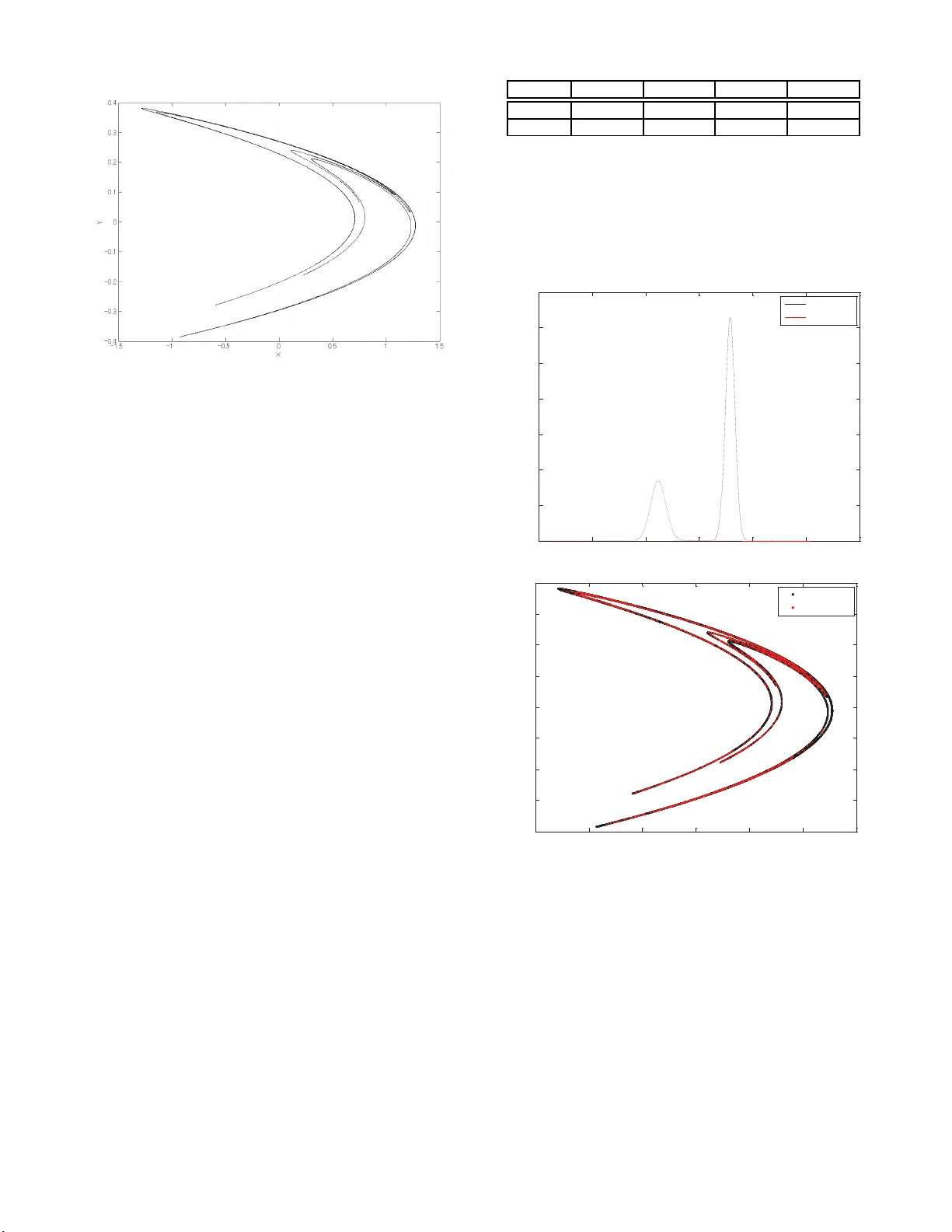
On the Estimation of P oin t wise Dimension ∗ Shohei Hidak a † and Neera j Kash yap † Scho ol of Know le dge Scienc e Jap an A dvanc e Institute of Scienc e and T e chnolo gy (Dated: July 4, 2018 ) Our goal in this pap er is to develop an eﬀective estimator of fractal dimension. W e survey existing ideas in dimension estimation, with a focu s on the currently p opular metho d of Grassb erger and Procaccia f or the estimation of correlation dimension. There are tw o ma jor diﬃculties in estimation based on this metho d. The ﬁrst is the insensitivity of correlation dimension itself to diﬀerences in dimensionalit y ov er data, whic h we term dimension blindness . The second comes from the reliance of th e metho d on the inference of limiting b ehavior from ﬁnite data. W e prop ose p oint wise dimension as an ob jec t for estimation in resp onse t o the dimension b lindness of correlation dimension. Po int wise dimension is a local q uantit y , and the distribution of p oint wise dimensions ov er the data contains the information to which correlati on dimension is blind . W e use a “limit-free” description of p ointw ise dimension to develop a new estimator. W e conclude by discussing p otential applications of our estimator as wel l as some chal lenges it raises. CONTENTS I. In tro duction 1 II. Mathematical Background 2 A. Poin twise Dimension 2 B. Other notions of dimensio n 4 1. Hausdorﬀ dimensio n 4 2. Box-coun ting dimension 4 3. Correla tio n Dimension 5 C. Dimensions o f Meas ures 6 II I. Numer ical Estima tion 7 A. The data 7 B. Grassb erger -Pro ca c cia E stimators 8 C. Analysis 8 IV. The E stimator 8 A. Guiding Principles 8 B. A limit-free description of p o int wis e dimension 9 C. Algorithm O verview 10 1. Glossary 11 2. The Ob jective 12 D. The V ariational Bay esian Algorithm 12 1. Phases 12 2. The Ob jective F unction 12 3. The Prio r Distributions 12 4. The Fixed Phase 13 5. The Clustering Phase 14 E. Implemen tation 15 V. Basic Ana lysis 16 A. Overview 16 ∗ This study w as supported by the NeuroCreative Lab, Grant-in- Aid for Scientiﬁc Researc h B No. 23300099 , and Grant -in- Aid for E xplor atory Research No. 2 5560297. † h ttp://www.jaist.ac.jp/˜shhidak a B. T est Data 16 1. dimension blindness 16 2. T ransformation Inv ariance 17 C. Results 17 VI. Op en Questio ns 19 A. Overview 19 B. F undamen tal Challenges in Dimensio n Estimation 19 C. Dimension and Dynamica l Systems 20 D. Detection o f Sto chastic Eﬀects 23 References 24 I. INTRO DUCT ION Dimension has b ecome an imp orta n t to ol in the study o f dynamical s ystems. Its imp ortance ar ises from the attempt to understand dy namical s ytems b y their attractors . The dimensions of these attractors provide useful in v ariants o f the systems in question. There are many no tions of dimension that one can consider in this context. The most well-known of these is Hausdorﬀ dimension. Hausdor ﬀ dimension, how ever, is diﬃcult to estimate num erica lly and this has given r ise to ma n y of the o ther conceptions . Often, o ne ca n asso cia te with erg o dic sys tems certain probability measures supp orted on a ttractors of in teres t. There is a dimension theory for probability measures, roughly analogous to the classic al dimensio n theory for sets, which one can bring to b ea r in the context of such systems. This is the setting for this pap er. In particular, we fo cus on the pro blem of estimating the p ointwise dimension di stribution of a probability measur e by sampling fro m it. In Section I I, we discuss v a rious mathematica l notions of dimension and the r elationships be t ween them. 2 In Section I I I , we disc uss the cur rent most p opu- lar tec hnique for estimating fractal dimension – that of Grassb erg er a nd Pr o caccia [1]. This discus s ion motiv a tes o ur deriv a tio n of our estima- tor of p o int wis e dimensio n, which we present in Section IV. In Section V, we establish a cer tain degree of r eliability of the es tima to r prop osed in Section IV by per forming a dimensional a nalysis of some test data. Finally , in Section VI, we discuss p otential applications of o ur estimator as well as certain theoretical questions arising fro m our considera tio ns. II. MA THEMA TICAL BACKG ROUND A. Poin t wise Dim ension V ery g enerally , the purp ose of any notio n of dimension is to tell apart certain t yp es of ob jects given a cer ta in notion of e quiv alence o f suc h ob jects. Point wise dimen- sion tells apart Borel probability measure o n metric spaces which are no t equiv alent b y a lo ca lly bi-Lipschitz injection. T o b e pr ecise let µ 1 and µ 2 be Borel proba bilit y mea - sures o n the metric space s ( X 1 , ρ 1 ) and ( X 2 , ρ 2 ) re spe c - tively . F or a p oint x in a metric s pace ( X , ρ ) and a num- ber ǫ > 0 , let us write B ( x, ǫ ) := { y ∈ X | ρ ( y , x ) < ǫ } . A map f : X 1 → X 2 is called lo c al ly bi-Lipschitz if for all x ∈ X 1 there exists r > 0 and a co nstant K ≥ 1 such that for all u, v ∈ B ( x, r ) we hav e 1 K ρ 1 ( u, v ) ≤ ρ 2 ( f ( u ) , f ( v )) ≤ K ρ 1 ( u, v ) . Let us s ay that the mea sures µ 1 and µ 2 are e quivalent if there exists a lo cally bi-Lipschitz injection f : X 1 → X 2 such that for all µ 2 -measurable U ⊂ X 2 we have µ 1 ( f − 1 ( U )) = µ 2 ( U ) . (1) Poin twise dimension is a source of inv aria nt s of s uch probability mea s ures under this notion of equiv a lence. Rather t han prov e this general statement, we will illustrate this in a very simple situation which motiv ates the concept of p oint wise dimension. The illustratio n will contain a ll the ideas require for the ge neral pro of. Consider the unit int erv al I a long with its uniform measure ν 1 and the unit square I × I a long with its uni- form mea sure ν 2 = ν 1 × ν 1 , bo th under their natural E u- clidean metrics. The “p oint wise dimension” metho d of telling these measures apar t is to obser ve that, for x ∈ I , we have ν 1 ( B ( x, ǫ )) ∼ ǫ, whereas, for y ∈ I × I , we hav e ν 2 ( B ( y , ǫ )) ∼ ǫ 2 . (2) If there w ere an equiv a lence f be tw een ν 1 and ν 2 , then we would hav e B  x, 1 K ǫ  ⊆ f − 1 ( B ( f ( x ) , ǫ )) ⊆ B ( x, K ǫ ) . This would force ν 1 ( f − 1 ( B ( f ( x ) , ǫ ))) ∼ ǫ, which would contradict (2). F or a general Bo rel pro bability measure, gr owth r a tes such as the ones we computed abov e for ν 1 and ν 2 may not exist at a ll p oints or even a t any point in the co r- resp onding metric space. This motiv ates the following deﬁnition: Deﬁnition 1. L et µ b e a Bor el pr ob ability me asur e on a metric sp ac e ( X , ρ ) . The lower p ointwise dimension of µ at x is deﬁne d to b e D µ ( x ) := lim inf ǫ → 0 log µ ( B ( x, ǫ )) log ǫ . (3) The u pp er p ointwise dimension of µ at x is deﬁne d to b e D µ ( x ) := lim sup ǫ → 0 log µ ( B ( x, ǫ )) log ǫ . (4) If these two quantities agr e e, we c al l t he c ommon value the p ointwise dimension of µ at x and denote it D µ ( x ) . The calculatio ns w e p erfo r med highlight t wo properties of p oint wise dimension: 1. P oint wise dimensio n is inv aria n t under bi-Lipsc hitz injections. 2. If µ is a bsolutely con tin uous with respect to Leb esgue measure o n R N , then the p oint wise di- mension of µ at any point in its supp ort is N . Let us now see ho w p oint wise dimension behaves for other cla s ses of measures. W e beg in b y considering the Cantor measure – this is the mea sure r esulting from the Cantor middle-thirds construction if at each scale we choose one of the remaining in terv als uniformly . T o b e precise, for a n interv al I , let u I denote the uniform mea - sure on I . At the n th stage of the middle third construc- tion, there are 2 n admissible interv al I ( n ) 1 , I ( n ) 2 , . . . , I ( n ) 2 n . Let us write ξ n := 1 2 n 2 n X j =1 u I ( n ) j . There is a limiting measur e ξ for the f amily { ξ n } which we ca ll the Cantor measure. ξ is supp or ted on the 3 Cantor set C . F or x ∈ C and ǫ > 0 , let us ﬁr st calculate ξ ( B ( x, ǫ )). Note that the s cale of this ball in terms of the middle- thirds c onstruction is given by log 1 / 3 ( ǫ ). This means that 2 −⌈ log 1 / 3 ( ǫ ) ⌉ ≤ ξ ( B ( x, ǫ )) ≤ 2 −⌊ log 1 / 3 ( ǫ ) ⌋ . This shows that log( ξ ( B ( x, ǫ ))) log( ǫ ) ∼ log 3 ( ǫ ) · log(2) log( ǫ ) , which in turn proves that D ξ ( x ) exists and is equal to log(2) log(3) . Of cours e , the Cantor mea s ure is a sp ecial case of a muc h more gener al class of measur es which we call Cantor-like me asur es . This cla ss o f meas ur es w as ﬁrst studied by Billingsley in the context of dimension theory [2, 3 ]. W e restrict our attention here to the ca se of Bo rel probability measure on R and esse ntially repro duce Billingsley’s deﬁnition here. It is po ssible to give a mo re mo dern deﬁnition in terms of iterated function sys tems . Let k > 0 b e an integer and le t π = ( p 1 , p 2 , . . . , p k ) be a probability vector. Divide the unit interv al I into k subin terv a ls o f equal length I 1 , I 2 , . . . , I k . Using our notation for the uniform measur e fr om b efor e, we write ξ π , 1 := k X j =1 p j u I j . W e can further sub divide each of the interv als I j int o k subint erv als o f equal length I j, 1 , I j, 2 , . . . , I j,k . This allows us de ﬁne ξ π , 2 := k X j 1 =1 p j 1 k X j 2 =1 p j 2 u I j 1 ,j 2 . Iterating this pr o cedure n times y ields a pro bability measure ξ π ,n . The family { ξ π ,n } has a limiting measure which w e denote ξ π and which generalizes our earlier construction of the Can tor measure. W e will now calculate the p o int wis e dimensio n of suc h a measure ξ π at a p oint x ∈ I . A p oint x ∈ I is uniquely sp eciﬁed b y a sequence of int eger s { j i } as { x } = ∞ \ i =1 I j 1 ,j 2 ,...,j i . Let ǫ > 0 . The scale of the ball B ( x, ǫ ) in terms of the construction of ξ π is given by log 1 /k ( ǫ ). In fact, if we write s ( ǫ ) := ⌊ log 1 /k ( ǫ ) ⌋ a nd S ( ǫ ) := ⌈ lo g 1 /k ( ǫ ) ⌉ S ( ǫ ) Y i =1 p j i ≤ ξ π ( B ( x, ǫ )) ≤ s ( ǫ ) Y i =1 p j i . (5) Let us count, for 1 ≤ j ≤ k , f n ( j ) := |{ i | 1 ≤ i ≤ n , j i = j }| . F ro m (5), we s ee that log( ξ π ( B ( x, ǫ ))) log( ǫ ) ∼ k X j =1 f S ( ǫ ) ( j ) log( p j ) log( ǫ ) . (6) Let us deno te by A π the set of x ∈ I for which, as ǫ → 0, f S ( ǫ ) ( j ) log( ǫ ) → p j log(1 /k ) . Then ξ π ( A π ) = 1 b y the strong law of larg e num ber s. Therefore, almost everywhere with r esp e ct to the mea- sure ξ π , we hav e D ξ π ( x ) = − 1 log( k ) k X j =1 p j log ( p j ) . (7) F urther more, fro m (6), we can see that there are in- ﬁnitely many p o int s in the supp ort o f ξ π at which its po in twise dimension is not deﬁned. W e illustrate this idea with the following example: Put n 1 := 1 . F or each integer m > 1, deﬁne n m := min  n | n − n m − 1 n > 1 − 1 2 m  . Let I denote the vector space of measur es generated by u [ a,b ] for a < b in R . Let us deﬁne S : I → I by S u [ a,b ] := 1 2  u [ a, b − a 5 ] + u [ b − b − a 5 ,b ]  . Let us deﬁne T : I → I by T u [ a,b ] := 1 3  u [ a, b − a 5 ] + u [ a +2 b − a 5 ,a +3 b − a 5 ] + u [ b − b − a 5 ,b ]  . Finally , put µ 2 m +1 := S n 2 m +1 T n 2 m · · · T n 2 S n 1 · u [0 , 1] , and µ 2 m := T n 2 m S n 2 m − 1 · · · T n 2 S n 1 · u [0 , 1] . Then each measure µ k is a Borel pro ba bilit y measure and the family { µ k } co nv erges to a B orel probability measur e µ . It is eas y to see tha t, for every po in t x in the supp ort of µ , we hav e D µ ( x ) = 1 2 log(2) log(5) , whereas D µ ( x ) = 1 3 log(3) log(5) , 4 Therefore, at no point in the support of µ do es it hav e a well-deﬁned p oint wise dimension. Mor e se r ious examples of such patho lo gical b ehavior have b een g iven by Ledr appier a nd Misiurewicz [4], a nd Cutler [5]. Although ther e is m uc h left to b e said on the matter of p oint wise dimension, w e end this section here hoping that we hav e given the rea ders enough of sense o f this quantit y that he is comfor table working with it. B. Other notions of dimensi on 1. Hausdorﬀ di m ension One of the most w ell-known notio ns of dimension is that of Hausdor ﬀ [6]. The notion of Hausdorﬀ dimensio n is built up on the notion of a Hausdo r ﬀ measure. Let E ⊆ R N , and let ǫ > 0. An ǫ - c overing of E is a countable co llection { E k } k of sets suc h that E ⊆ ∪ k E k and sup k diam( E k ) ≤ ǫ . F or ǫ > 0 , put H α ( E , ǫ ) := inf { E k } ( X k diam( E k ) α    { E k } k ) , (8) where the inﬁmum is ov er ǫ -coverings { E k } of E . Then Hausdorﬀ α - mea sure ( α > 0) is deﬁned by H α ( E ) := lim ǫ → 0 H α ( E , ǫ ) . (9) Note that this limit either exists or is ∞ b ecause H α ( E , ǫ ) is a no n-increasing function of ǫ . Observe that, for α < β , we hav e the inequality H β ( E , ǫ ) ≤ ǫ β − α H α ( E , ǫ ) . Suppo se that H α ( E ) ∈ (0 , ∞ ). Then allowing ǫ → 0 in the a b ove inequality for ces H β ( E ) = 0. Therefore there exists a unique critical exp onent α such that H β ( E ) =  0 , β > α ∞ , β < α . (10) Deﬁnition 2. F or a set E ⊂ R N , we c al l the un ique exp onent α satisfying (10) its Hausdor ﬀ dimension , and denote it by D H ( E ) . This exp onent α is deﬁned to b e the Hausdorﬀ dimen- sion D H ( E ) of the set E . Hausdor ﬀ dimension has the following prop erties: 1. Hausdorﬀ dimensio n is in v a riant under lo cally bi- Lipschitz injections, 2. for a decomp osition of E in to countably many se ts E = ∪ k E k , we hav e D H ( E ) = sup { D H ( E k ) } , 3. the Hausdor ﬀ dimensio n o f a ball in R N is N . Broadly sp eak ing, Haus dorﬀ dimension provides a measure of co mplexit y for sets which is more ﬁnely stratiﬁed than, say , Leb esgue measure. F or e xample, the Cantor se t has Leb esgue meaur e zero but Hausdor ﬀ dimension log(2) / log(3). This makes Hausdorﬀ dimen- sion a very useful to ol in the sciences. W e no w discuss certain development s around Ha usdorﬀ dimension in the nu merica l study o f dynamica l systems. Although there is no rigor o us cr iterion b y which one may class ify a set as fractal, a fractio na l Hausdorﬀ dimension is one impo rtant indicator of suc h structure. As a co nsequence, Hausdo rﬀ dimension ha s long been used to detect chaotic b ehavior in dyanamical s y stems (see, for exa mple, Ott [7]). F or example, the Hausdorﬀ dimension of a smo oth attrac to r is a geometric inv ariant and therefor e one may use it to classify such a ttractors. In practice, Haus dorﬀ dimensio n is diﬃcult to estimate from data. One o f th e reasons for this is the deﬁnition of the Hausdorﬀ α -meas ures themselves (Eq. 9). Given a set E , eﬀective estimation of H α ( E ) requir es o ne to pro duce an ǫ -cov ering of E which is clo se to optimal. The problem with this is that at diﬀer en t place s in E such an ǫ -cov ering would employ sets of diﬀeren t diam- eters. F ur ther more, it is diﬃcult to identify the c ritical exp onent α with only estimates o f the α - measures. This is one r eason that Hausdorﬀ dimension is diﬃcult to estimate. Another reas o n comes from prop erty 2 of Hausdorﬀ dimension listed ab ov e. The s et of po int s in E which dictate its Hausdorﬀ dimensio n may be rela- tively “ small” whic h presents diﬃculty in the estimation. Most n umerica l estimators of dimension have sought to ev ade these diﬃculties b y estimating instead qua n tities which mer ely provides approximations to Ha usdorﬀ di- mension. The most well-kno wn of these appr oximations are capacity or b ox-counting dimension, cor relation di- mension, and information dimension. W e now pr esent each o f these in turn alo ng with some estimators. 2. Box-c ounting di mension The idea b ehind box-counting dimension is that the dimension of a set is related to as ymptotic behavior of the num b er o f cub es of side length ǫ req uired to cov er it as ǫ → 0 . F or example, for ǫ > 0, o ne r equire ǫ − N cube s of side length ǫ to cov er the unit cub e in R N . This allows us to recover the dimension N as N = lim ǫ → 0 log( ǫ − N ) log( ǫ − 1 ) . This motiv ates the fo llowing gener al deﬁnition: Deﬁnition 3. Le t E ⊂ R N . L et us denote by B ( E , ǫ ) the minimal numb er of cub es (or ‘b oxes’) of side length ǫ r e quir e to c over E . 5 We deﬁne the lower b ox-c ounting dimension of E by D B ( E ) := lim inf ǫ → 0 log( B ( E , ǫ )) log( ǫ − 1 ) . Similarly, we deﬁne the u pp er b ox-c ounting dimension of E by D B ( E ) := lim sup ǫ → 0 log( B ( E , ǫ )) log( ǫ − 1 ) . If these quantities agr e e, we c al l the c ommon value the box-counting dimens io n of E , and denote it by D B ( E ) . If, in the deﬁnition of Hausdorﬀ dimension, w e take the inﬁmum in (8) ov er cov ers { E k } of E wher e each E k has a diameter e xactly ǫ , and if the corres po nding limit (9) ex ists, we recov er the b ox-counting dimension o f E . Incident ally , the above relationship b et ween the deﬁni- tions of Haus dorﬀ dimension and b ox-counting dimension shows that, for any E ⊂ R N , D H ( E ) ≤ D B ( E ) . (11) F re q uen tly , it is the cas e tha t the inequality in (11) is an equality . I n a sense, it is the situations in whic h the inequality is strict which make b ox-counting dimension a po o r no tion of dimension. F or example, b ox-counting dimension do es not sa tisfy anything lik e P rop erty (2) of Haus dorﬀ dimension – one cannot calculate the box- counting dimension of a s et using a countable decomp o- sition of that s et. As an illustratio n, let Q := Q ∩ I . As Q is dense in I , an y co vering o f Q by ǫ -balls m ust also cov er I . Therefor e, D B ( Q ) = D B ( I ) = 1. On the o ther hand, if we enumerate Q and write Q = [ k { q k } , we have D B ( { q k } ) = 0 for all k . Despite its ﬂaws, b ox-coun ting dimension r emains p op- ular becaus e it is s o ea sy to estimate. W e will discuss the estimation of b ox-counting dimension in Section I II . 3. Corr elation Di mension Grassb erg er and Pro ca c cia, in [1 ], pr op osed a metho d of estimation of fractal dimensio n. How ever, it was not originally clea r what kind of dimension they were estimating. Since then this notion has b een formalized to pro duce what we know to day as c orr elation dimension – see, for exa mple, P esin [8]. In this section, we give a brief account of this historica l developmen t. The basic idea o f Grassb er ger and Pro c accia was very similar to the idea whic h motiv a ted our description of po in twise dimension in Sectio n I I A. The pr oblem that they considere d was that of e s timating some kind of fractal dimension for an attracto r in a dy na mical system given a ﬁnite n umber of iterates of so me initial v alues. They reasoned that the rate at which the ca rdinality of intersections of ǫ -balls a round the data p oints with the data decayed w ould provide a reasona ble notion of dimension provided that such a r a te was well-deﬁned. T o b e precise, given the data E = { x 1 , x 2 , . . . , x n } ⊂ R N , let us ﬁx a norm k · k o n R N , and deﬁne the c orr elation sum C ( E , ǫ ) := 1 n n X i =1   1 n − 1 X j 6 = i χ [0 ,ǫ ) ( k x i − x j k )   , (12) where χ [0 ,ǫ ) denotes the characteristic function o f the int erv al [0 , ǫ ). Gra ssb erger and Pro caccia [1] suggested that estimating the rate of decay o f C ( E , ǫ ) with ǫ would provide a go o d notion of dimensio n for the set E . While this technique was in some sens e v ery e a sy to a pply numerically , it lac ked a rigorous mathematical foundation – ther e was no known notion of dimensio n that the Grassb erger -Pro ca c c ia metho d (GP ) could b e prov ed to provide an estimate of in general. Implicitly , Grassb erg er and Pr o caccia had introduced a completely new no tion of dimension – correlation dimension. The previously cited pap er o f Pesin [8] de velops co rrelation dimension from a v ague conc e pt to a r igorous quantit y . One diﬃculty in forma lizing the c o ncept of co rrelation dimension is that cor relation s ums (12) ar e deﬁned for ﬁnite sets of data. F o r example, this preven ts us from deﬁning the correla tion dimension as simply a limit of the correlation sums a s ǫ → 0. In fa c t, this particular p oint in tro duces muc h diﬃculty even in nu merica l estimation. W e will discus s this in detail in Secton I I I. F or the purp os es o f r igoro us for m ulation, another problem with the ﬁniteness of data is that it is not clea r wha t kind of underlying pro cess o f data generation one should consider when trying to deﬁne correla tion dimensio n. In this pap er, we will a ssume that the data is sampled according to a pr obability meas ure µ , and therefor e we deﬁne the co rrelation dimension of µ . Let µ b e a probability measure, and let { X j } be a sequence of indep endent rando m v ar iables with distribu- tion µ . Let us deﬁne E n := { X 1 , X 2 , . . . , X n } . Then, for a ﬁxed ǫ > 0 , the limit C ( µ, ǫ ) := lim n →∞ C ( E n , ǫ ) (13) exists almost surely by the strong law of la rge num be r s, and is equal to the pro bability that k X 1 − X 2 k < ǫ . 6 Deﬁnition 4 . The limit D C ( µ ) := lim ǫ → 0 log( C ( µ, ǫ )) log( ǫ ) , if it exists, is c al le d the c o rrelatio n dimensio n of µ . If µ is a Borel pr obability mea sure on R N , then let us write for x ∈ R N F µ,ǫ ( x ) := µ ( B ( x, ǫ )) . In this ca s e, we hav e C ( µ, ǫ ) = k F µ,ǫ k 1 , and so D C ( µ ) = lim ǫ → 0 log( k F µ,ǫ k 1 ) log( ǫ ) . This sugg ests that there is a n en tire family of dimensio n related to the correla tion dimension. T he s e dimensions are ca lled the q - generalized dimensio ns , were ﬁrst intro- duced by Hen tschel a nd Pr o caccia [9 ] in a manner similar to that in whic h c o rrelation dimension was intro duced by Grassb erg er and Pro caccia [1]. F o rmally , w e deﬁne the q -gener a lized dimension of µ , if it exists, to b e D C,q ( µ ) := lim ǫ → 0 log( k F µ,ǫ k q − 1 ) log( ǫ ) . (14) W e take the norm in L q − 1 ( µ ) ab ov e in order to b e consistent with the nota tion used in the n umerical literature. The re a son for this c o nv en tion is appar en t from the deriv ation of Hent schel and P ro caccia [9]. In this pa per , we will b e concer ned mainly with the correla tion dimensio n although muc h of o ur discussion of c o rrelatio n dimensio n ca rries over directly to the case of the q -generalized dimension. Note that, in deﬁnition, there is quite a bit of similarity betw een the c orrelatio n dimension of µ (Deﬁnition 4) and its p oint wise dimension at some gene r ic point x in its suppo rt (Deﬁnition 1). F or example, Cutler [1 0] deﬁnes the aver age p ointwise dimension of a Bore l probability measure µ on R N by D P ( µ ) := Z R N D µ ( x ) d µ ( x ) . She p oints out that, while D P ( µ ) reﬂec ts the av erage o f the lo cal rates of dec ay of the measur e of ǫ - balls ar ound po in ts in the supp ort o f µ , D C ( µ ) r eﬂects the rate o f decay of the average measur e of ǫ -balls around po int s in the suppor t of µ . This seems to ha ve b een a sour ce o f confusion in the past. W e urg e the reader to b e wary bo th in rea ding ab out and applying these concepts. T o expa nd upo n this, supp ose that for each i = 1 , 2 we hav e a Bor el pr obability measure µ i on R N with as so ci- ated ǫ i > 0 such that fo r each 0 < ǫ < ǫ i we hav e µ i ( B ( x, ǫ )) ∼ ǫ α i . Let us further a ssume that the supp orts of µ 1 and µ 2 are contained in disjoint op en sets in R N and that α 1 < α 2 . Finally , let us de ﬁne µ = 1 2 µ 1 + 1 2 µ 2 . As we will see in (16), for each i = 1 , 2 , we hav e D C ( µ i ) = α i . Now, we also hav e, for ǫ > 0, C ( µ, ǫ ) = 1 2 C ( µ 1 , ǫ ) + 1 2 C ( µ 2 , ǫ ) . Thu s, for 0 < ǫ < min( ǫ 1 , ǫ 2 ), we have C ( µ, ǫ ) ∼ 1 2 ǫ α 1  1 + ǫ α 2 − α 1  . Therefore, D C ( µ ) = lim ǫ → 0 log( ǫ α 1 ) + log (1 + ǫ α 2 − α 1 ) log( ǫ ) = α 1 . (15) This alrea dy hig hlights one of the ma jor pro blems with correla tion dimension – it cannot even b e used to tell apart a s imple mixture of measur es such as µ fr o m its low est dimensional component! W e call this the dimen- sion blindness of co rrelation dimensio n. This p o ses a se- rious problem with relying up on estimators of cor relation dimension in the analysis of data. W e seek to address this problem with our estimator . C. Dime ns i ons of Me a s ures Although Hausdorﬀ dimension pr ovides a measur e of complexity of sets , as w e ha ve deﬁned it, it is easy to derive fro m it a notion of dimension for measures. W e follow he r e the developmen t of Cutler [10]. Deﬁnition 5. Le t µ b e a Bor el pr ob ability me asur e on R N . We deﬁne the Hausdorﬀ dimension distribution µ H of µ , which is a Bor el pr ob ability me asu r e on [0 , N ] , by µ H ([0 , α ]) := sup { µ ( E ) | D H ( E ) ≤ α } . We deﬁne the H aus dorﬀ dimension of µ to b e D H ( µ ) := inf { α ∈ [0 , N ] | µ H ([0 , α ]) = 1 } . A t this p oint, we hav e descr ibed in some detail three notions of dimension asso ciated with a Borel probability measure µ o n R N – p oint wise dimension, co rrelation di- mension, and Hausdo rﬀ dimension. A lot is known ab out the relationships b etw een these three dimensions, pa rtic- ularly w hen µ has c onstant p oint wise dimension D µ ( x ) = d, 7 for almos t every x in its suppor t. Y oung [1 1] prov ed that, when this is the case, we have D H ( µ ) = d. Pesin [8] proved that, in the sa me case, we hav e D C ( µ ) = d. (16) In fact, the results of Y o ung a nd Pesin are a bit mo r e general. Cutler ha s explored in g r eater detail the rela- tionship b etw een the distribution of p oint wise dimensions of µ a nd its co r resp onding Hausdorﬀ dimension distribu- tion µ H : Theorem 1 (Cutler [10], Theore m 3.2 .2) . Le t µ b e a Bor el pr ob ability me asur e on R N . L et us c onsider the fol lowing subset of the s u pp ort of µ : D α := { x | D µ ( x ) ≤ α } . Then D H ( D α ) ≤ α , a nd µ H ([0 , α ]) = µ ( D α ) . T o give a r ough idea of the kind of rea soning required to prove these results, let us consider (16). Supp ose that µ sa tisﬁes the following co ndition: there ex ist co nstants c, C > 0 and ǫ 0 > 0 s uc h tha t, for all po in ts x in the suppo rt of µ and all 0 < ǫ < ǫ 0 , cǫ d < µ ( B ( x, ǫ )) < C ǫ d . (17) Then it is ea s y to see that D C ( µ ) = d as, fo r 0 < ǫ < ǫ 0 , we have cǫ d < C ( µ, ǫ ) < C ǫ d . F or a gener al Borel proba bilit y measur e µ with a lmo st everywhere constant p oint wise dimension d , t here is no such garantee of uniformity in lo c al scaling . The trick to proving the ge neral r esult is to obser ve that any such measure can b e written as a limit of measur es satisfying the condition (17). T o see this, we can restr ic t µ to those po in ts in its support at which the condition is satisﬁed for v arious v a lues of c, C, and ǫ 0 . µ is a limit of such restrictions. The condition that µ has consta n t p oint wis e dimension almost everywhere in its support is not an exceptional one as far a s dyna mical data is concerned – for example, if µ is er g o dic for a map f , then this c o ndition is satisﬁed under q uite general constra in ts o n f . F or more details, refer to Cutler ([5, 12]). W e state here a simpliﬁed version of Cutler ’s res ults: Prop ositio n 1. L et f : X → X b e a lo c al ly bi-Lipschitz, er go dic map with er go dic me asur e µ for which t he p oint- wise dimension exist s almo st everywher e. Then µ has c onst ant p ointwise dimension almost everywher e in its supp ort. Pr o of. Since µ is inv ar ia nt under f , f deﬁnes an equiv a- lence b etw een µ and itself in the sense of (1) in Sec tio n II A. This tells us that the function D µ ( x ) is f -inv ariant. As f is er go dic, this means that D µ ( x ) is consta nt. This ca n form the basis for a test of ergo dicity . W e will dis c us s this in Section VI C. II I. NUMERICAL EST IMA TION In this section, w e demonstrate how one ma y use the idea of Grassb erg e r and Pro ca ccia [1] to estimate the cor relation dimensio n of a measur e . W e call suc h metho ds GP estimators . Currently , GP estimator s seem to b e the most freq uen tly used estimator s of fractal dimension in the applied sciences. W e b egin by presenting the data to which we will apply the estima tor, along with a theoretica l a nalysis. W e then descr ibe how one would desig n a GP estimato r for this data. W e present the results of an ana lysis of the data with suc h an e stimator. Finally , we co nclude by discussing some of the dra wbacks of GP estimators. This will mo tiv ate our estimator of p oint wise dimensio n, which we prese nt in the next section. A. The data W e will use three measures in our demonstr a tion of the GP estimato r. The ﬁrst pr obability measure that we use is the Cantor measure ξ , which w e deﬁned in Section II A. The seco nd measure we use is ζ := 1 2 ( ξ + ξ ′ ) , where ξ ′ is the meas ur e der ived from ξ by mapping the int erv al [0 , 1] linea rly onto [2 , 7 ]. This repres en ts the im- age of ξ under a piecewis e linear transformation. The third mea sure that we use is a mixture of tw o measures with diﬀerent dimensio na l b ehavior: η := 1 3 δ 0 × ξ + 2 3 ( ξ ∗ δ 1 ) × ( ξ ∗ δ 1 ) , where δ α denotes the p oint-mass at α ∈ R . Before w e b egin our ana ly sis, we must calculate the correla tion dimensions of ea ch of these measur es. The calculation for the ﬁrst t wo measures follo ws from (16) upo n observing that the po in twise dimension of those measures is equal to log(2) / log (3) a lmost everywhere in their supp orts. F or the mea s ure η , observe that D C ( δ 0 × ξ ) = log(2) log(3) , and D C (( ξ ∗ δ 1 ) × ( ξ ∗ δ 1 )) = 2 log(2) log(3) . The calculatio n of the corr elation dimensio n of η essen- tially follows the calculatio n (15), a nd we hav e D C ( η ) = log(2) log(3) . Once ag a in, dimension blindness rea rs its ugly hea d. Still, it is interesting to see how it manifests itself in nu merica l estimation. 8 B. Grassbe rger-Procaccia Estimators Suppo se that w e are giv en a da taset D of n points sampled from a Bo rel pr obability measure µ on R N , and that we wish to use this data to estimate the c orrelatio n dimension of µ . The basic idea in a ny GP estimator of correlatio n dimensio n is to use the co rrelation sums deﬁned in (12) at v ar ious sca les to p e rform this esti- mation a ccording to Deﬁnition 4. Since the data is only av ailable at a coarse resolution, so me delica cy is required in inferr ing the limiting b ehavior of the corr ela- tion sums from the few which are av aila ble fro m the data. What one often do es is ev aluate correlatio n sums at v ar ious s c ales, de c ide s which ra nge o f scale s contains the most information ab out the correlation dimension, and ﬁnally use a linear mo del to estimate the quantit y log( C ( µ, ǫ )) log( ǫ ) ov er this range. This burden on the analyst to c ho ose an informative range of scales is pro blematic as it can po ten tially b e a larg e sour ce o f bias in the analys is. W e will exp erie nce the diﬃcult y of making this choice in our analysis of the test data. C. Analysi s (a) The Cantor Measure x log e log e log e Correlation Dimension Correlation Dimension Correlation Dimension (b) Scale Mixture z (c) Dimension Mixture h FIG. 1. The GP estimator (a) on a dataset sampled from the 1-dimensional Cantor set and (c) on a d ataset sampled from an ob ject whic h is mixture of 1- and 2-dimenisonal Cantor set. (b) The GP estimator on th e same dataset as (a) t ransformed with a p iecewise linear function. In Figure 1, we presen t graphs of log( C ( µ, ǫ )) a s functions of lo g( ǫ ) for ea ch o f the measure µ = ξ , ζ , η of Section I I I A. W e sampled 10,00 0 p oints from eac h measure up to a pr e cision of 3 0 ternary digits for this analysis. W e have indicated our choices of informative regions on e a ch gra ph by shading them. The hor i- zontal line reﬂects the true correla tion dimension of log(2) / log (3) in each graph. Observe that, after ta k ing logs o f the co r relation sums and the para meters ǫ , the infor mative r ange of scales is the one o ver which the regression line for the data is closes t to hor iz ontal and the total lea s t square er ror is relatively s ma ll. It is diﬃcult to state more precise criterion for choos ing this region. F or example, in Figure 1(b), there seems to be no cle a r choice of informative scaling reg ion. F ro m Figure 1, we obtain the following estimates (the ground truth is log(2 ) / log(3) = 0 . 630 9 3): 1. D C ( ξ ) ≈ 0 . 6305 ± 0 . 041 1 , 2. D C ( ζ ) ≈ 0 . 5859 ± 0 . 0066, 3. D C ( η ) ≈ 0 . 7411 ± 0 . 0 194. F ro m Figure 1(c), o ne may b e tempted to claim that the eﬀects of the mixture are o bserv a ble – there is a distinct bump in the graph over the range 10 − 11 < log( ǫ ) < 10 − 10 . Suc h a claim is not eas ily justiﬁable, ho wev er, for the sa me b ehavior is present in Figure 1(a). Figure 1(b) is of pa rticular interest, for it shows that the GP e s timates of c orrelatio n dimension ar e not sensi- tive ev en to piecewise linea r transfo r mations of the data . IV. THE ESTIMA TOR A. Guiding Principl e s W e obser ved, in Section I I I, some of diﬃculties in- volv ed in estimating dimension using a GP estimator. Broadly , these diﬃculties arise fro m tw o so urces: 1. The dimension blindness o f cor relation dimension. 2. The o nu s on the user to choo se co rrect s c ale in ana l- ysis. These ar e imp ortant issues to address when desig ning a new estimator . Bearing in mind the dimension blindness of correla - tion dimension, it see ms desirable to instead estimate a dimension which is more sens itiv e to the lo ca l str uc tur e of a given probability measure. Therefor e , we choose to estimate point wise dimension. This enables us to tr e at the dimension as a distribution, which has certain sta- tistical adv antages b eyond the elimination o f blindness of v ar ying dimensions. This will become clear in our nu merica l analys is of the estimator. Overcoming the problem of the s ensitivity of data to scale is m uch more diﬃcult. The reason that this 9 sensitivity is such a pro ble m in GP estimators is that Grassb erg er and Pr o caccia [1] explicitly dep end up on limiting b ehavior to pr o duce go o d estimates. Addressing this problem in the ca se of an estimator of p oint wise dimension is not ea sy b e c ause p o int wis e dimension is fundamen tally a lo ca l quan tity . W e utilize the idea that distances of data points to their near est neig h b ors contain informatio n ab out lo c a l dimensions o f the measure that the da ta is sa mpled from. W e expand upo n this idea in more detail in the next section. Finally , attempting to estimate point wise dimension carries with it certain diﬃcult ies which a re not presen t when estimating correlation dimension. The principal problem is that to get a true sense of distribution of po in twise dimensio ns ov er the da ta can b e computation- ally v ery exp ensive. As a result of this computatio nal diﬃcult y , although s ch emes to estimate point wise dimen- sion hav e previously been suggested (for example, Cutler [10]), there has b een no larg e s cale implement ation that we a re aw ar e o f. In our e stimator, w e utilize clustering techn iques to mitigate this cost. The idea is to identify data p oints at which the underlying measure seems to ha ve simila r sc a ling prop erties. W e discuss this in greater deta il in Section IV C and IV D. Finally , one situation in whic h it was diﬃcult to choose scale s for analysis was when the da ta had bee n transfor med by a lo cally bi-Lipschitz injection. Although we hav e not emphasized this p oint very muc h in o ur discussio n so far, it was a pr imary motiv ation in developing our estimator. As p oint wise dimension is purely lo cal qua ntit y , an estimator of p oint wise dimension should naturally b e less sensitive to the eﬀects of suc h tr ansformations. In fact, we inco rp orate such insensitivity to lo cal scaling in our e stimator in the form of lo cal density pa rameters, this is certa inly something that the re ader sho uld b e aw are of as the pro ceed thro ugh this pap er. T o summarize, there a r e fo ur p oints that the reader should keep in mind thr o ughout the rest of this pap er: 1. P o i n t wise dime nsion : W e estimate p oint wise di- mension, which is sensitive to diﬀerence s in sca ling behavior over the data. 2. Limit-free de scription : W e utilize a limit-free description of p oint wise dimension, which makes estimation mor e eﬀective. 3. T ransformation in v ariance : W e introduce a lo- cal density para meter which gives our estimator the ﬂexibility to cop e with data which has b een tr ans- formed by a lo ca lly bi-Lipschitz injection. 4. Clustering : W e use clustering techniques to iden- tify data p oints with similar po in twise dimension characteristics, which sav es on computational cost. B. A l i mit-free description of p oint wise di mension In this section, we dev elop an estimator of point wise dimension which utilizes the distance s from data p oints to their nea rest ne ig hbors. The distributions of these distances ar e approximated by waiting time distributions for Poisson pro cess es. Such appr oximations pr ovide an eﬀectiv e mea ns of estimation for a larg e cla s s of generating measures µ . Cutler and Dawson [13, 14] hav e similar results for diﬀerent clas ses o f measures using very diﬀerent techniques. Let us b egin b y considering a Borel probability mea- sure µ which sa tis ﬁe s the following lo c al un iformity c on- dition : Suppo se that the po in twise dimension D µ ( x ) is deﬁned at every p oint x in the suppo rt of µ . Supp ose further that, at every suc h point x , there is a constant δ x > 0 and ǫ ′ > 0 such that, fo r all 0 < ǫ < ǫ ′ , µ ( B ( x, ǫ )) = δ x ǫ D µ ( x ) . (18) The main diﬃcult y in obtaining the limit-free de- scription o f D µ ( x ) is that it is diﬃcult to ma ke gener al statements about the inﬁnitesimal behavior of µ at x . W e will show that, as far a s measures satisfying the lo c a l uniformity co ndition are co ncerned, one may obtain eﬀective estimates of p oint wise dimension b y assuming that the inﬁnitesimal b ehavior is that of a Poisson pro cess. Let µ b e a B orel probability measure o n R N satisfying the lo cal uniformity condition (18) ab ove, and supp ose we would like to estimate D µ ( x ) given some data sampled from µ . Let us say tha t the question of whether or not there is a data p oint at distance r from x is determined by a Poisson pr o cess Z ( r ) with ra te δ x r D µ ( x ) . E xplicitly Z ( r ) counts the num be r n of da ta p oints at dista nce up to r from x , a nd ha s density function. ζ ( n ) = δ n x r nD µ ( x ) n ! exp  − δ r D µ ( x )  (19) Let us deﬁne, for n > 0, the waiting times R n ( x ) := sup { r > 0 | Z ( r ) < n } . These ar e the distances fro m x to its n th nearest da ta po in ts. T he pro bability densities of the random v ariables R n ( x ) c a n b e easily calculated fr om that of Z ( r ) as φ n ( r ) = D µ ( x ) δ n x r nD µ ( x ) − 1 ( n − 1)! exp  − δ x r D µ ( x )  . (20) The sp ecial cas e n = 1 has b een der ived in Cutler a s a log gamma distribution ([15]; See also [10] Deﬁnition 7.2.1) and [16]. The essentially same for m as (19) is also used by Nerenberg and Essex [17] in the context of erro r analysis co rrelation dimensio n. 10 Since µ satis ﬁes the local uniformity condition, it lo oks like a uniform measur e in a small ball around x . Sp eciﬁcally , it loo ks like a uniform measure which arises from the Poisson pr o cess described ab ov e by conditioning on the region where the data is sampled. As a result, the distribution corres po nding to (2 0) is a go o d approximation to the true nea rest neigh b or distribution at s mall scales . This mea ns that, if the data is ﬁne enoug h, (20) pr ovides an eﬀective way of estimating the p oint wis e dimensio n. As we will see in our a nalysis o f our estimator , this sensitivit y to scale of the a pproximation is not very marked. W e end this se c tio n by showing how the limit-free de- scription we hav e given a bove cor resp onds to a more con- ven tional deriv ation of p oint wise dimension. Let us denote the distribution function of (20) by F n ( r ) = R r 0 φ n ( r ) d r . Sp eciﬁcally , it is given b y an in- complete gamma function: F n ( r ) = Z δr D µ ( x ) 0 t n − 1 exp( − t ) d t. (21) In fact, F n ( r ) gives the same asymptotic scaling be- havior a s µ . Namely , using LHopital’s rule, we g e t lim r → 0 1 n log F n ( r ) log r = D µ ( x ) . (22) As the densities δ x are allo wed to v ary , and s ince w e are trying to estimate the distribution of po int wise di- mensions of µ , it will b e useful for us to distinguish b e- t ween the distributions F n ( r ) co rresp onding to diﬀerent choices of pa rameters in (18). Ther e fore, we cons ider the conditional dis tributions F n ( r | δ x , D µ ( x )) . W e denote their cor resp onding probability density func- tions by φ n ( r | δ x , D µ ( x )) . In pra ctice, the sample pro bability density is often a b e tter approximation to the tr ue probability den- sity of the dis tribution b eing sampled from than the sample dis tribution is of the distribution. Thus we seek to appr oximate the proba bilit y density functions φ n ( r | δ x , D µ ( x )) from the data g iven to us. F or a given n , we call the estimate this gives us for D µ ( x ) the n th ne ar est-n eighb or dimension . As we hav e s e en, the n th nearest-neig h b or dimensio ns provide go o d estimates to p oint wise dimensions for mea- sures satisfying the local unifor mit y condition (18) . W e remark that there are certa inly patholog ical measures for whic h this condition does not hold – for e xample, the measures deﬁned in Billing sley [3], which C utler [10] terms “ fractal meas ures”. It is an in teresting proble m to determine how one may give a limit -free description of po in twise dimension in the case of such measures. As a ﬁnal po in t of note, it is the densities δ x in this description which ena bles us to build into our alg orithm the desired insensitivity to lo cally bi-Lipschitz injections of the data which we discuss ed in the previous section. C. Algorithm Overview Suppo se that we are g iven a sequence D = { x 1 , x 2 , . . . , x k } in R N of da ta sampled from a B orel pr obablity mea sure µ . F or each 1 ≤ j ≤ k and each 1 ≤ i < k , let us denote by r j ( i ) the distance fro m x j to its i th closest neig h b or in D . F or each 1 ≤ i < k , we deﬁne the s e q uence R i := { r 1 ( i ) , r 2 ( i ) , . . . , r k ( i ) } . In our algor ithm, a parameter n is sp eciﬁed a t the outset. Our goal will be to use the n th -nearest neigh- bo r distances R n of the data D in order to obtain an approximation µ = M X m =1 θ m µ m , (23) where 1. 0 < θ m ≤ 1 , P M j =1 θ m = 1. 2. Eac h µ m is a B orel probability mea s ure satisfying the lo ca l uniformity condition of (18). 3. Eac h measure µ m has constant p oint wise dimension d m = D µ m ( x ) and consta n t density δ m = δ x for all po in ts x in its suppo rt. 4. The measures µ m hav e disjoint suppo rts. Given (23), we ca n par tition the data D into M clusters deﬁned by the supp orts of the measures µ m . θ m represents the prop or tion of the data in the cluster K m corres p onding to µ m . The quality of an appr oximation of the type sp eciﬁed by (2 3) depe nds on the c hoice of M . F or example, if M = 1, then any dimension estimate derived from the approximation reﬂects an aggrega te o f th e lo cal scaling behaviors of µ around the data points. On the o ther hand, if M = k (the size o f the data D ), then one o btains a clear picture of the individual sca ling b ehaviors, but at great co st. Often it is not necessary to go to this latter extr eme in order to estimate the distribution of p oint wise dimensions o f µ at the da ta po in ts. An impo rtant feature of our algo rithm is that it chooses the clusters and the num b er of clusters adaptively , balancing 11 concerns o f eﬃciency with those of clarity . W e will describ e this in grea ter detail in Section IV D 5. The big ger pr oblem is a ctually pro ducing the mea- sures µ m . In o rder to do this, we will use a V ariatio nal Bay esian method. The idea is that, since each µ m satisﬁes the lo cal unifor mit y condition (18) with con- stant dimensio n and density , the n th -nearest neighbor distribution for e a ch cluster K m of the da ta should have a probability density function which is appr oximately φ n from (20) for the appropr iate c hoice of parameters d m and δ m . As a part of this pro cedure, we use the density functions φ n to pr o duce p oster ior distr ibutions for the para meters d m and δ m having ma de a choice of prior distributions. It is imp o rtant to note that this forces us to treat the dimension d m (as well a s the other parameters ) implicitly as random v ariables . It is also worth noting that the choice of prior dis tributions for the relev ant par ameters can hav e a marked impac t on the p e r formance of the estimato r when the da ta is sparse. The cluster parameters – the n umber of clusters M , the cluster ass ignment s K m , and consequently the w eights θ m – are estimated co ncurrently with the pa rameters d m and δ m . In or der to do t his, we make use of the laten t cluster a s signment v ariables Z im :=  1 , if x i ∈ K m , 0 , else . Most of the optimization in our alg o rithm is condi- tioned on the num b er o f clusters M . In these steps, the v ar iables that we seek to estimate from the data are d m , δ m , and θ m . O ur estimates for the v ar iables Z i,m are derived from thos e. Th us we r e quire prio r distributions for d m , δ m , and θ m . W e assume that the v ariables d m and δ m follow indep endent gamma distribution with the parameter ( α d , β d ) and ( α δ , β δ ) respe c tiv ely . F o r each in- teger M > 0, we a ssume that the vector ( θ 1 , θ 2 , . . . , θ M ) follows a Dirichlet distributio n with the pa r ameter  γ ( M ) 1 , γ ( M ) 2 , . . . , γ ( M ) M  . Figure 2 provides a graphical mo del depicting the dependency b etw een these v ariables. 1. Glossary Data: • D — a sequence x 1 , x 2 , . . . , x k of k data points in R N sampled fro m the Bor el proba bilit y measure µ for w hich we a re trying to estimate the distribution of p oint wise dimensions . • R n — the seq uenc e o f distanc e s r 1 , r 2 , . . . , r k from each o f the data p oints in D to its n th -nearest neigh- bo r. Basic v ariables used in estim ation: Data m d n m d m q i r Cluster m d a d b im Z d a d b Hyper parameters Density W eight Dimension n -NN distance m g M Q Basic variables M W M Cluster assignment Number of clusters N R FIG. 2. Dep endencies among th e v ariables. • M — the num b er of cluster s in the approximation (23). • θ m — the weight of cluster m in (23). • d m — the p oint wise dimensio n o f µ m in (23). • δ m — the density para meter in the Poisson pro cess approximating µ m according to the dis cussion in Section IV B. • Z im — the indicator that the i th data p oint in D belo ngs to cluster m . Hyp er-parameters: • ( α d , β d ) — the pa r ameters for the gamma pr ior of the dimensio n par ameter d m . • ( α δ , β δ ) — the par ameters for the gamma prior o f the density pa rameter δ m . • γ ( M ) := ( γ ( M ) 1 , . . . , γ ( M ) M ) — the parameters for the Dirichlet prior of the weigh t par ameters θ ( M ) := ( θ 1 , . . . , θ M ). Some sho rt-hand: • Θ M = (( Z im ) , ( d m ) , ( δ m ) , ( θ m )) — a list of the ba- sic v ar iables apar t from M . • Θ = ( M , Θ M ) — the list of a ll the basic v aria ble s . • Ω M =  ( α d , β d ) , ( α δ , β δ ) , ( γ ( M ) 1 , . . . , γ ( M ) M )  — the list of hyper-par ameters for a ﬁxed num ber M o f clusters. • Ω = ( M , Ω M ) — here, the n umber of clusters is allow ed to v a r y . 12 2. The Obje ctive The goa l of the pr o cedure descr ibe d abov e is to com- pute the p o sterior distr ibution for the list of v ariables Θ given Ω and R N : P (Θ | Ω , R N ) = P ( R N | Θ) P (Θ | Ω) P ( R N | Ω) . (24) D. The V ariational Bayesian Al gorithm 1. Phases As we hav e a clea n description (20) of the relation- ship b etw een the bas ic v ariables, we ca n feasibly use the v ar iational Bay esian metho d presen ted b y Jor dan et al. [18 – 21] to estimate the p oster io r distribution (2 4 ). There are t wo distinct pha ses in our application o f this metho d: • The ﬁxed phase — here, we estimate the po ste- rior distribution conditioned upon the n umber of clusters M . • The clus te ring phase — here, we use the tech- niques o f Ueda et al. [2 2, 2 3] to ﬁnd the num b er of clusters M for which the estimate from the corre- sp onding ﬁxed phase b est appr oximates the po ste- rior of (24). Although we treat thes e phases separately , there is considerable b etw e en them as we itera tively up date our estimate of the p osterior (24). In the following sectio n, we describ e the co nnection betw een the tw o phases of our pro cedur e – the ob jective function that our estimator seeks to maximize. 2. The Obje ctive F unction A t ea ch step, and for e ach comp onent X of Θ, we dis- tinguish b etw een the true marg inal p os terior distribution P ( X | Ω , R N ) derived from (24) a nd our estimates o f this distribution Q ( X | Ω), which we a lso denote Q ( X ) for con- venience as we a re not v ar ying the hyp e r-para meter s Ω. Finally , this is crucial, w e ass ume that these marginal distributions of Q ar e independent for ea ch ﬁxed num ber of c lus ters M : Q (Θ M ) = k Y i =1 Q ( θ ( M ) ) M Y m =1 Q ( Z im ) Q ( d m ) Q ( δ m ) . (25) W e can e s timate the quality of the a pproximation Q by considering the likelihoo d P ( R N | Ω) which measur e s how well the data is determined by the hyper- pa rameters Ω. T o b egin with, log P ( R N | Ω M ) = lo g Z P ( R N , Θ M | Ω M ) dΘ M . Let us write L M ( Q ) = Z Q (Θ M ) log P ( R N , Θ M | Ω M ) Q (Θ M ) dΘ , (26) and let us denote by κ M ( Q ) the Kullback-Leibler diver- gence κ M ( Q ) := K L ( Q (Θ M ) k P (Θ M , R N | Ω M )) . (27) W e hav e the decomp osition log P ( R N | Ω M ) = L M ( Q ) + κ M ( Q ) . (28) Our go al, in the ﬁxed pha se o f the pro cedure, is to ﬁnd the distribution Q which maximizes the ob jectiv e function L M ( Q ). This is equiv a lent from the above decomp osition to minimizing the Kullback-Leibler divergence κ M ( Q ), whic h measur es the error in o ur approximation. In our implementation, w e use the explicit des cription of the ob jectiv e functions L M ( Q ) to perfor m the opti- mization. W e will describ e the details for each of the phases s e parately once we ha ve presented explicit de- scriptions of the rele v ant prior distributions, whic h the following sectio n is devoted to. 3. The Prior Distributions In this section, we present ex pr essions for the prior distributions P ( X | Ω M ) which w e will make use of in our implement ation. W e also describ e the distribution of the data conditioned on the basic v ariable s P ( R N | Θ M ) which w e use in conjunction with the pr iors to derive the p oster ior distribution P (Θ M | Ω M , R N ). W e b egin by describing our assumed pr ior distributions for the basic pa rameters g iven a ﬁxed nu mber of clusters M . W e stated o ur assumptions ab out these pa r ameters at the end of Section IV C, but we provide her e ex plic it expressions of their pro ba bilit y densities: 1. T he density parameters — The density param- eter δ m is ass umed to follow a gamma distribution with the shap e parameter α δ > 0 and the rate pa- rameter β δ > 0: P ( δ m | α δ , β δ ) = β α δ δ δ α δ − 1 m Γ( α δ ) exp ( − β δ δ m ) . (29) 2. T he dimension parameters — The dimension parameter d m is assumed to follow a ga mma distri- bution α d > 0 and β d > 0: P ( d m | α d , β d ) = β α d d d α d − 1 m Γ( α d ) exp ( − β d d m ) . (30) 13 3. The w eig h t parameters — The weigh t par am- eter θ := θ ( M ) follows a Dirichlet distribution with the exp one nts γ := γ ( M ) : P ( θ | γ ) = Γ  P M m =1 γ m  Q M m =1 Γ( γ m ) M Y m =1 θ γ m − 1 m . (31) 4. The cluster in di cators — The cluster indicators Z i := ( Z i 1 , Z i 2 , . . . , Z iM ) follow a multinomial dis- tribution with the probabilities θ : P ( Z i | θ ) = M Y m =1 θ Z im m (32) Finally , the conditional proba bilit y o f drawing the sam- ples R N given a set of basic v aria ble s Θ M is P ( R N | Θ M ) = N Y i =1 M Y m =1 n θ ( M ) m P ( r i | n, δ m , d m ) o Z im (33) where P ( r i | n, δ m , d m ) = d m δ n m r nd m − 1 i Γ( n ) exp  − δ r d m i  . (34) Note tha t (33) and (34 ) ar e derived fro m (20), a ccount- ing for diﬀerences in the clusters. The ab ov e expressions allo w us to explicitly describ e the o b jectiv e function (26). This desc r iption is provided in (35), and is developed in the following section. 4. The Fixe d Phase Recall that in the ﬁxed phase of our a lgorithm we ﬁx a num b er of c lus ters M and attempt to ﬁnd an approximate p osterio r dis tr ibution Q ( X ) for each comp onent X o f Θ M . This a pproximation is obtained by itera tively ma x imizing the ob jectiv e function L M ( Q ). In this sec tio n, we describ e what happ ens in a single iteration of this optimizatio n pro ce dur e. W e denote by Q t the approximation obtained at the t th step, a nd w e also introduce the notation Θ M , ¬ X for those comp onents of Θ M which are dis tinct fro m X . Each step of the optimization is further divided into four p ortio ns. These p ortions co rresp ond to the four classes of basic parameters distinct from the n umber o f clusters M – the density par ameters δ m , the dimension parameters d m , the w eight parameter s θ = θ ( M ) , a nd the cluster indica tors Z i = ( Z i 1 , Z i 2 , . . . , Z iM ). In eac h po rtion, we mo dify the v alues of the r elev ant parameters conditioned up on thos e of the o ther classes of parame- ters. The goal at each step is to increase the v alue of the ob jectiv e function L M ( Q ), s o that we alwa ys hav e L M ( Q t ) ≤ L M ( Q t +1 ) . The co nv ergence of such metho ds has b een studied extensively by Attias [19], a nd by Ghahra mani and Beal [21], a lthough it has not b een rigo rously prov en. Stated plainly , our go al is to approximate the true dis- tributions of the ba s ic v ariables δ m , d m , θ , and Z i from within a co nstrained family o f po sterior distributions. In our approximation, we will assume that the densities δ m follow a gamma distribution, that the weigh ts θ follow a Dirichlet distribution, and that the cluster indicator s Z i follow a multin omia l distr ibution. The p oster iors for the dimensions will be derived from our estimated p oster iors of these v ariables . Th us, at step t , the situation is as follows: 1. The estimated po sterior dis tr ibution Q t ( δ m ) is a gamma distribution with the estimated parameter s ˆ α ( t ) m and ˆ β ( t ) m . 2. The estimated p osterior distributio n Q t ( θ ) is a Dirichlet distribution with the estimated parame- ters ˆ γ ( t ) =  ˆ γ ( t ) 1 , ˆ γ ( t ) 2 , . . . , ˆ γ ( t ) M  . 3. The estimated p osterio r distribution Q t ( Z i ) is a m ultinomial distribution with the estimated pa- rameters ˆ π ( t ) i :=  ˆ π ( t ) i 1 , ˆ π ( t ) i 2 , . . . , ˆ π ( t ) iM  . 4. The estima ted p osterior distribution Q t ( d m ) is de- rived from the abov e p oster ior distributio ns in a manner that we shall describ e b elow. This distri- bution has the parameter s ˆ A ( t ) m , ˆ B ( t ) m , and ˆ C ( t ) im for 1 ≤ i ≤ N , and its probability density function is Q t ( d m ) = d ˆ A ( t ) m m ˆ D ( t ) m exp d m ˆ B ( t ) m − N X i =1 ˆ C ( t ) im r d m i ! (36) where the denominato r ˆ D ( t ) m normalizes the integral of (3 6). W e will need ano ther bit of notation b efore w e can describ e the rules by which we up date the p osterior dis- tributions. F or a comp onent X of Θ M and a function f of X , we write f ( X ) ( t ) := E Q t ( X ) [ f ( X )] , the exp ectatio n of f ( X ) with resp ect to the v ariationa l po sterior distr ibutio n Q t ( X ). W e now present the up date r ules. These rules ar e de- rived from the pro cedur e pres ent ed in Jor dan et al. [18], and we refer the reader to that pape r for details. Accord- ing to [18], for each co mponent X of Θ M ∗ , the up dating rule for the v a riational p osterio r is written with (33): Q t +1 ( X ) ∝ P ( X | Ω M ) e E Q t (Θ M, ¬ X ) [log( P ( R n | Θ M ))] (37) Pseudo-co de cor resp onding to each rule may be found in Section IV E . In parentheses, we name ea ch upda ting 14 L M ( Q ) = k X i M X m =1 Z im ( t )  − log  Z im ( t )  + log ( θ m ) ( t ) + log( d m ) ( t ) + nd m ( t ) log( r i ) + n log( δ m ) ( t ) − δ m ( t ) r d m i ( t )  − k log Γ( n ) − M X m =1 log Γ ( γ m ) + log Γ M X m =1 γ m ! + M log  β α δ δ Γ( α δ )  + M log  β α d d Γ( α d )  (35) + M X m =1 log Γ  ˆ γ ( t ) m  − log M X m =1 Γ  ˆ γ ( t ) m  ! − M X m =1 n ˆ α ( t ) m log  ˆ β ( t ) m  − log  Γ  ˆ α ( t ) m  − ˆ β ( t ) m δ m ( t ) o + M X m =1 ˆ D ( t ) m rule for use in our pseudo - co de in Section IV E. Up date rule s for ˆ α ( t ) m and ˆ β ( t ) m ( P osteriorDensity in Section IV E) ˆ α ( t +1) m := α δ + n k X i =1 Z im ( t ) , and ˆ β ( t +1) m := β δ + k X i =1 Z im ( t ) r d m i ( t ) . Up date rule s for ˆ γ ( t ) ( P osteriorW e igh t in Section IV E) ˆ γ ( t +1) m := γ ( M ) m + k X i =1 Z im ( t ) . (38) Up date rule s for ˆ π ( t ) ( P osteriorCluste r in Section IV E) log  ˆ π ( t +1) m  ∝ log ( θ m ) ( t ) + log ( d m ) ( t ) (39) + n d m ( t ) log( r i ) + n log ( δ m ) ( t ) (40) + δ m ( t ) log ( d m ) ( t ) . (41) Here, we have δ m ( t ) = ˆ α ( t ) m ˆ β ( t ) m , log ( θ m ) ( t ) = Ψ  ˆ γ ( t ) m  − Ψ M X m =1 ˆ γ ( t ) m ! , and log ( δ m ) ( t ) = Ψ  ˆ α ( t ) m  − log ˆ β ( t ) m , where Ψ( x ) = d d x log(Γ( x )) is the digamma function. The o ther exp ectations do not hav e such simple expres- sions a nd are estimated numerically . Up date rule s for ˆ A ( t ) m , ˆ B ( t ) m , a nd ˆ C ( t ) im ( P osteriorDimen s ion in Se c tion IV E) Upda ting r ule of the dimension parameter d m ( (P osteriorDimen- sion) in Section IV E). ˆ A ( t +1) m = k X i =1 Z im ( t ) + α d − 1 , ˆ B ( t +1) m = n N X i =1 Z im ( t ) log r i + β d , and ˆ C ( t +1) im = δ m ( t ) Z im ( t ) . The denomina tor ˆ D ( t +1) m of (36) is numerically inte- grated. This denominator plays an importa n t role in the ev aluation of the ob jectiv e function L M ( Q ) as seen in (35). Its num eric a l es timation is a bottleneck in our algorithm. This co ncludes our disc us sion of the ﬁxed phase of our algorithm. W e now discuss the choice of the n umber of clusters M . 5. The Cl ustering Phase In this section, we discuss ho w we adaptively choos e the num b er o f clusters M in the approximation (2 3) using the split-and-mer ge technique of Ueda et a l. [22, 23]. W e describ e here the essence of this method and refer the reader to those pap er s for details. F or a given approximation o f the for m (23), there are many wa ys in whic h one could potentially split or merge clusters . In the cur rent implementation of our alg orithm, we hav e essentially chosen to attempt splits and mer ges at random. T her e is a quite bit of scop e for improv ement in this depa rtment. How ever, for the rest of this section, let us assume that w e hav e either chosen a cluster to split or chosen tw o clusters to mer g e together witho ut concer ning ours elves with ho w the choice was ma de . Thus, fro m the orig - inal list of M clusters, we are considering whether or 15 not to use M ∗ clusters wher e M ∗ is either M − 1 or M + 1 . In either ca s e, we b egin by adjusting the h yp er- parameter γ ( M ) . In the case of a prop osed split, γ ( M ∗ ) is deriv ed from γ ( M ) by distributing the c ompo nent corres p onding to the cluster to be split ev enly among the t wo new clusters. In the case o f a prop o sed merg e , the comp onent co rresp onding to the cluster to b e merged are simply a dded together to pro duce that o f the new clus ter. The next step is to ass ig n v alues to the par ameters for the v ar iational pos teriors o f the densities and dimensions which w e descr ibed in the previo us section. F o r most of the clusters, these parameters will remain unchanged in the new mo del. In the case where w e are consider- ing a split, one of the new clusters will have the same parameter v a lues as the origina l cluster wher eas the sec - ond new cluster will hav e parameter v alues whic h are per turbations of these v alues. In the ca se where w e a re considering a merg e, the pa rameter v alues for the new cluster is the average o f those for the o riginal clusters . Once these v alues have b een assigned, w e use the up- dating rules presen ted in the previous s ection to der ive v ar iational p oster ior distr ibutions Q ∗ for the basic v ari- ables conditioned on the n umber of cluster s b eing M ∗ . This allows us to compa re the v a lues of the ob jectiv e functions L M ( Q ) a nd L M ∗ ( Q ∗ ) using (26). W e accept the pr o po sed split or mer ge if L M ∗ ( Q ∗ ) > L M ( Q ) . F urther technical de ta ils of our implementation a re clear from the pseudo-co de in Section IV E, where the clustering phas e is presented in the form o f the functions Split a nd Merge . E. Implementation The ﬁrst problem we address in o ur implementation is that of initializing the basic v ar iables. W e be g in by assuming that ther e is only one cluster – M = 1. Under this assumption, we use the maximum likelihoo d estimates of the ba sic v aria ble s corresp onding to the conditional distribution P ( R n | Θ 1 ) derived in (33). The bas ic v a riables ca n also b e initialized under the assumption that the initial num b er of clusters is s ome ﬁxed num b e r larger than 1. In this situation, we use the EM alg orithm of Dempster et a l. [2 4]. The next issue is of deciding when the optimization pro cedure should halt. Our implementation ta kes an argument t max , which sp eciﬁes the ma ximal num be r of iterations to p erform. It also takes a n ar g ument ∆ L , which sp eciﬁes the minimum a cceptable improvemen t in the v alue of the ob jectiv e function. If w e de no te b y L t the v alue of the ob jectiv e function a t step t , the pro g ram halts if t = t max or L t − L t − 1 < ∆ L . The pseudo-co de b elow deta ils our implementation un- der these co nditio ns. The Main function takes the data, the num b er n of nea rest neighbors to b e used, and the ini- tial num b er o f clus ters as arguments. It calls each of the functions Up date , Split , and Merge iteratively , chec k- ing fo r the halting criteria at each step. The function Up date implements the ﬁxed phase of o ur algorithm, and the clustering phase is handled by Split and M erge . The Ob jectiv e function ev aluates the ob jective func- tion L M ( Q ) for a given lis t of basic v ariables . The functions who se names beg in with ‘ P osterior ’ are im- plement ation of the update rules which ma y be found in Sectio n IV D 4. The LogNormal function r e tur ns a sample from the log-no rmal distribution with the sp eciﬁed mea n and v ariance parameters. The function Random ( { 1 , . . . , M } , k ) r andomly choo ses a subset of { 1 , 2 , . . . , M } of size k . 1: Main ( D , n, M , ∆ L , t max ) 2: R n ← NearestNeighborDistances ( D , n ) 3: { d m , δ m , θ m , Z im } ← Initiali zation ( R n , M ) 4: L 0 ← inf 5: L 1 ← 0 6: Θ M ← ( { d m , δ m , θ m , Z m } M m =1 ) 7: while | L t − L t +1 | > ∆ L and t ≤ t max do 8: t ← t + 1 9: ( L t , Θ M ) ← Upd ate (Θ M ) 10: ( ¯ L t , ¯ Ω M − 1 ) ← Merge (Θ M } M m =1 ) 11: if ¯ L t > L t then 12: L t ← ¯ L t , Θ M − 1 ← ¯ Ω M − 1 , M ← M − 1 13: end i f 14: ( ¯ L t , ¯ Ω M +1 ) ← Spli t (Θ M ) 15: if ¯ L t > L t then 16: L t ← ¯ L t , Θ M +1 ← ¯ Ω M +1 , M ← M + 1 17: end i f 18: end whi le 19: return (Θ M ) 1: Up date (Θ M = { d m , δ m , θ m , Z im } M m =1 ) 2: Initialize: t = 0, L 0 ← −∞ , L 1 ← 0 3: while | L t − L t +1 | > ∆ L do 4: t ← t + 1 5: { d m } ← P oste ri orDimensio n ( { δ m , θ m , Z im } M m =1 ) 6: { δ m } ← P o s teriorDensity ( { d m , θ m , Z im } M m =1 ) 7: { θ m } ← P o s teriorW ei g h t ( { d m , δ m , Z im } M m =1 ) 8: { Z im } ← P oste ri orCluster ( { d m , δ m , θ m } M m =1 ) 9: L t ← Ob jectiv e ( { d m , δ m , θ m , Z im } M m =1 ) 10: end whi le 11: Θ M ← { d m , δ m , θ m , Z im } M m =1 12: return ( L t , Θ M ) 1: Split (Θ M = { d m , δ m , θ m , Z im } M m =1 ) 2: K ← Random ( { 1 , . . . , M } , 1) 3: Θ K ← { d m , δ m , θ m , Z im } m ∈ K 4: ( L, Θ 2 ) ← Upd ate ( Initi alizeSplit (Θ K )) 5: Θ M +1 ← { Θ 2 , Θ M \ Θ K } 6: return ( L, Θ M +1 ) 16 1: Merge (Θ M = { d m , δ m , θ m , Z im } M m =1 ) 2: if M = 1 then 3: return ( −∞ , Θ M ) 4: end i f 5: K ← Random ( { 1 , . . . , M } , 2) 6: Θ K ← { d m , δ m , θ m , Z im } m ∈ K 7: ( L, Θ 1 ) ← Up date ( InitializeMerge (Θ K )) 8: Θ M − 1 ← { Θ 1 , Θ M \ Θ K } 9: return ( L, Θ M − 1 ) 1: NearestNeighborDis tances ( D , n ) 2: Use the KD-tree algo rithm to compute the list of n th - nearest neighbor dis tances R n of the data points in D . 3: return R n 1: Initialization ( R n , M ) 2: Use the E M alg orithm to estimate the initial parame- ters { ¯ d m , ¯ δ m , ¯ θ m , ¯ Z im } which max imize the likeliho o d P ( R n | Θ M ). 3: return { ¯ d m , ¯ δ m , ¯ θ m , ¯ Z im } 1: InitializeSpli t (Θ 0 = { d 0 , δ 0 , θ 0 , Z i 0 } ) 2: for m = 1 , 2 do 3: d m ← d 0 × LogNormal (0 , σ ) 4: δ m ← δ 0 × LogNormal (0 , σ ) 5: θ m ← θ 0 × LogNormal (0 , σ ) 6: Z im ← P osteriorCl us ter ( { d m , δ m , θ m } ) 7: end fo r 8: Θ 2 = { d m , δ m , θ m , Z im } 2 m =1 9: return (Θ 2 ) 1: InitializeMerge (Θ M = { d m , δ m , θ m , Z im } M m =1 ) 2: d 0 ← 1 M P M m =1 d m , δ 0 ← 1 M P M m =1 δ m 3: θ 0 ← P M m =1 θ m , Z i 0 ← P M m =1 Z im 4: Θ 0 = { d 0 , δ 0 , θ 0 , Z i 0 } 5: return (Θ 0 ) V. BASIC A NA L YSIS A. Overview In this sec tion, w e test our estimator o n data sa mpled from cer ta in pro bability measures related to the Ca n tor measure. Recall that we pe rformed a s imila r ana lysis of GP estimator s in Section I I I C, a nd that we identiﬁ ed t wo serious issues a s a result: 1. The diﬃcult y in choos ing informative scales. 2. High sens itivit y to transforma tions of the data un- der which dimension is inv aria n t. There is one further thing tha t we observed – not only do es the diﬃculty in cho o sing informativ e scales r eﬂect the dimensio n blindness of cor relation dimension, but we also observed this same pr oblem for data sampled from the Cantor measure which ha s uniform p oint wise dimension. In this section, w e will analy ze the b ehavior o f our pro- po sed estimator when confronted with v ario us da ta sets that exhibit b ehavior whic h was problematic for the GP estimator w e analyzed in the manners descr ib ed ab ov e. While the problem of having to choos e informative scales has b een a ddressed in the des ign of o ur estimato r itself, the causes o f the o ther pro blems were muc h subtler a nd call for a de ta iled a nalysis. Before we p er fo rm o ur anal- ysis, we formally describ e the co rresp onding meas ures. B. T e s t Data Each of o ur test data sets is genera ted for the purp ose of studying the eﬀects on our e stimator of o ne of the tw o following pro blems: 1. Insensitivit y to distribution of p oint wise dimen- sions. 2. Sensitivit y to lo cally bi-Lipschitz injections. W e prese nt the data sets which test each of these issues in turn. 1. dimension blindness Our ﬁr st cla ss of measures is derived from the Cantor measure ξ (which we desc rib ed in detail in Section I I A). W e call these measures Cantor mixt u r es , and they are essentially conv ex combinations of pro ducts of the Can- tor measur e with itself. T he Cantor mixtures allow us to test to the sensitivity o f o ur estimator to the distribution of point wise dimensions of a genera ting measure. The goal is to see how susc eptible our estimator is to the problems ca used by dimension blindness in the case of GP estimato r s – the short a nswer is, “not very”. W e now describ e this cla ss explicitly: Cho ose positive integers M , N 1 , N 2 , . . . , N M , and N . Cho ose v ector s v (1) , v (2) , . . . , v ( M ) ∈ R N . F or v ∈ R N and 1 ≤ k ≤ N , let us write ξ v, k :=   k Y j =1 δ v j ∗ ξ   ×   N Y j = k +1 δ v j   . Finally , let π ∈ R M be a proba bilit y vector. W e ca ll the measure M X m =1 π m ξ v ( m ) ,N m (42) a Cantor mixtur e . 17 Basically , for each 1 ≤ m ≤ M , we are taking the N m -fold pr o duct of the Cantor set with itself, embedding it in to the ﬁrst N m co ordinates of R N , a nd translating it by the vector v ( m ) . The mea s ure ξ v ( m ) ,N m can b e constructed o n this set in the same way that we constructed the Can tor measure ξ . Finally , in order to get the Ca ntor mixture, w e sample from ξ v ( m ) ,N m with probability π m . In o ur analy sis, we a lwa ys choose v ( m ) = ( m, m, . . . , m ) ∈ R N . W e gener ate ﬁve data s ets: 1. Data set A consists of 10 ,000 p oints sa mpled from the Cantor measure up to 30 ternary dig its o f pre- cision. 2. Data set B consis ts of 1 0,000 p oints sampled from the mixture of the Ca n tor measur e a nd the ﬁve-fold pro duct of the Cantor measure with weights 2 / 3 and 1 / 3 resp ectively . 3. Data set C co nsists of 20 0 0 p oints sampled from the mixture o f the tw o-fold and three-fold pro ducts of the Cantor measur e with w eights 3 / 4 and 1 / 4 resp ectively . 4. Data set D cons ists of 10,0 00 p oints sampled fr o m the mixture of the Ca n tor measur e with its ﬁv e-fold and ten-fold pro ducts with w eights 1 / 7, 2 / 7, and 4 / 7 res pectively . 5. Data set E consists of 10 ,000 p oints sampled from the mixture of the Cantor measure with its tw o- fold, three-fold, and four-fold pro ducts, each with equal weight. The r esults of the analys is are pr esented in Section V C, and ar e summarized in T a ble I. 2. T r ansformation I nvarianc e T o test the degree of inv ariance of our estima to r to lo cally bi-Lipschitz injections, we use a class of measures which genera lize the measures ζ that we use d in the analysis of the GP es tima tor. Rather than deﬁning the measures here, w e ex plicitly desc r ibe the corresp onding sampling pr o cedures. W e b egin with some num ber k of linear functions f 1 ( x ) , f 2 ( x ) , . . . , f k ( x ) which satisﬁes the condition f j (1) ≤ f j +1 (0) , 1 ≤ j < k . T o g enerate a s a mple, we b egin by ﬁrst drawing a sample X from the Cantor measure. With probabilit y π k , o ur sample from the testing mea sure is f k ( X ). W e b egin with a pr o bability vector π = ( π 1 , π 2 , . . . , π k ). W e deﬁne, for 1 ≤ j ≤ k , σ j := j X i =1 π i and deﬁne σ 0 := 0. W e consider the linea r functions f j ( x ) o f slo pe 2 j − 1 satisfying f j ( σ j ) = f j +1 ( σ j ) , 1 ≤ j < k . W e draw a p oint X fro m the Ca n tor measure. With probability 1, there is unique 1 ≤ j ≤ k such that X ∈ [ σ j − 1 , σ j ]. The cor resp onding sample from the testing measur e, then, is f j ( X ). In our analysis , k r a nges fro m 1 to 5 a nd, for each k , we generate a hundred data sets, with each data set co ns ist- ing o f 1 0,000 samples . In ea ch ca s e, w e c ho ose the proba- bilit y vector π by drawing at ra ndom from the space of k - dimensional probability vectors acco rding to the Dirichlet distribution with the parameter (1 / 2 , 1 / 2 , . . . , 1 / 2). W e choose linear functions f j ( x ) o f slop e 2 j − 1 . The results of our analysis a re pr esented in the following section, and are summarize d in Figure 4 . C. Results In each o f the following ana lyses, we set the n umber of Euclide an nearest neighbors n = 1 , a nd the initial nu mber of clusters M = 1. The par ameters for the prior distributions ((29), (30), and (31)) a re ﬁxed to be α δ = α d = γ 1 = 1, and β δ = β d = 10 − 4 resp ectively . These are the only choices that we had to make for our estimator and, since our algo rithm adaptiv ely choo ses the n umber of clusters M , our initializatio n M = 1 is not rea lly a serious limitation. W e begin by prese nting the results of o ur analysis on the Cantor mixture data sets which we describ ed at the end of Sectio n V B 1. T a ble I co nt ains a summary which compares estima tes for the average p oint wise dimensio n of g enerating meas ur es using o ur estimato r on the given data sets with their true v alues. W e also show in the table the num b er o f clusters chosen by our estimato r for each data set, and the reader will see that this num b er of clusters agrees with the n um b er of measures in each mixture. In fact, the cluster a ssignments themselves are in line with the decomp ositions of ea ch of the Ca ntor mixtures into combinations of the pro ducts of the Cantor measure. Figure 3 demons tr ates that this is true in the cases of data sets D and E . In the ﬁgure, the p oints in the data sets ar e listed along the vertical axis, a nd the clusters are marked a long the horizontal ax is . The int ensity of the color c orresp onding to a particula r data po in t - cluster pair indicates the estimated pr obability that the given data point b elong to the given cluster, 18 with 0 being white and 1 being black. Of course, our algorithm estimates the a verage p oint wise dimensio n in each cluster s eparately . The results for each individ- ual clus ter in data s ets D and E a re presented in T able I I. The results inv olving the Cantor mixtures that we present exhibit the following general tre nds , which we hav e veriﬁed in mor e extensive exp eriments: 1. The erro rs in our estimates increase with the num- ber of comp onents in the mixtur es. 2. The err o rs in our estimates for n -fo ld pro ducts o f the Ca n tor mea sure increas e with n . 3. The error s in our estimates decreas e as the sample size incre a ses. 4. The more comp onents of similar dimens io n that there are in a mixtur e, the larg er we expe c t the error s in our estimates to b e. Of these four trends, the ﬁrst three are not at all s ur pris- ing. The four th calls for elab or ation. The clustering data for data set E provided in T able II and Figur e 3 shows that the estimator mistakes po int s s ampled from the t wo-fold a nd four-fold pr o ducts of the Can tor measure as having b een sampled from the three-fold pro duct. Note tha t there is co nsiderable physical separ ation in the data sampled from the v a rious co mp onents of the mixture. Rather, this e stimation error is a result of there being muc h more similarity b etw een these comp o nent s in ter ms of the nearest neighbo r distances . The pro blem of r educing the in terface betw een clusters as far as the nearest neigh b or data is concer ned does not s eem to b e out of reach. There are many paths that one could follow to attack th is pro blem – the choice of metric used to calcula te the near est neighbor distances surely ha s a signiﬁcant eﬀect, for example, or one might be able to simply analyze the re s ults of o ur estimator on each individual c luster pro po sed for the data set as a whole in or der to get an idea of how relia ble the orig inal cluster assig nments ar e. Regar dless of the method, any impro vemen t along these lines see ms to b e highly depe ndent on the particular da ta in question. W e feel that this is an imp orta n t co nsideration in data ana lysis, and w e hope that our estimator provides a useful to ol for its so lutio n. In o ur analys is of the sensitivity of our estimator to lo cally bi-Lipschitz injections, we used the data se ts describ ed at the end of Section V B 2. The results are summarized in Figure 4. Each of the generating meas ur es has uniform po int wise dimens io n log (2) / log(3) ≈ 0 . 63 09. This is indicated in the ﬁgur e by the r ed line. The horizontal ax is in the ﬁg ure represents the num b er k of regions of v ar ying density (these are the images of the v ar ious functions f j ). The v ertical axis re pr esents the estimated average p oint wise dimens ion. The vertical (a) Dataset D (3 clusters) (b) Dataset E (4 clusters) 1 2 3 1 2 3 4 Estimated cluster indices Estimated cluster indices Data point indices FIG. 3. The cluster assignment visualized by the gray-scal e color map. The black cell indicates probab ility 1, while one in- dicate probability 0, and gray ind icates in-b etw een. F or each case, the 10,000 data p oints are ind exed in an ascending order of its true dimension. The clusters are index ed correspond ing to T able I I. bars aro und our estimates reﬂect the standard error of the estima ted average p oint wise dimensions. Unsurpris- ingly , the es timates get worse a s the num b er of regions increases. How ever, even in the case k = 5, the estimate obtained from our estimator is not far from the true v alue log (2) / log(3). W e plan to expand up on this issue of transfo rmation inv ariance in a subseq uent pap er. N-piecewise linear transform ation Nearest Neighbor Dim ensions A verage Dimension Ground T ruth ( ) ( ) 3 log 2 log FIG. 4. T ransformation inv ariance With this, we conclude our discussio n of the estimato r itself. In the next sectio n we desc r ibe some potential uses of our estimator a s well as so me questions which we feel are imp ortant and which arise naturally fr om our discussion un til this p oint. 19 Data settings Estimation Dataset Sample size Clusters M N 1 , . . . , N M F requencies π A vg. P oint wise Dim. Avg. P oint wise D im. Clusters M A 10,000 1 1 ( 1) 0.63093 0. 63063 1 B 10,000 2 1, 5 (2 / 3 , 1 / 3) 1.4722 1.4474 2 C 2,000 2 2, 3 (3 / 4 , 1 / 4) 1.4196 1.4449 2 D 10,000 3 1, 5, 10 (1 / 7 , 2 / 7 , 4 / 7) 4.596 8 4.6875 3 E 10,000 4 1, 2, 3, 4 (1 / 4 , 1 / 4 , 1 / 4 , 1 / 4) 1 .5773 1.4460 4 T ABLE I . The summary of the analysis of the ﬁve Cantor mixture datasets Dataset D Cluster Index 1 2 3 Estimated W eight 0.1403 0.2798 0.5799 Estimated Dimension 0.6293 3.21 20 6.3811 S.D. of Dimension 0.0024 0.0090 0.0166 T rue W eigh t 0.1429 0.285 7 0.5 714 T rue Dimension 0.6309 3.154 6 6.3 093 Dataset E Cluster Index 1 2 3 4 Estimated W eight 0.2572 0.2069 0.3299 0.2059 Estimated D imension 0.6187 1.3876 1.4180 2.5825 S.D. of Dimension 0.0017 0.0037 0.0047 0.0084 T rue W eigh t 0.25 0.25 0. 25 0.25 T rue Dimension 0.6309 1.261 9 1.8 928 2.5237 T ABLE I I . The details of th e estimated parameters for Data set D and Data set E. The clusters are indexed in ascending order of its estimated av erage dimension within th e cluster. VI. OPEN QUESTIONS A. Overview W e hav e pr esented in this pap er a new technique for the numerical e s timation of fracta l dimensions. As such, the ma jority of the p otential for our metho d lies in ap- plying it to numerical data. How ever, in the dev elopment of our estimator, several fundamental questions about dimension estimation itself w ere raised, which share an int imate r elationship with these p otential a pplications. These questio ns concer n the applicability of our metho d and dimension estimation metho ds in genera l. W e will discuss these methods before moving on to a disc us sion of the p otential numerical scop e of o ur a lg orithm. There are a lso several technical improvemen ts that can p oten- tially be ma de to the e stimator that we hav e presented. Suggestions for such impro vemen ts ha ve b e e n scattered throughout the text. W e omit such questions in this section, preferring to focus on wha t w e consider to b e the ma jor challenges that our estima to r makes access ible. This section is rea lly mor e ab out what we do not know than what we know. W e do attempt, how e ver, to provide preliminary numerical results with each ca tegory of open questions that we discuss. Although we have presented our questio ns in diﬀerent categor ies, there is consider able int era ction b etw een them. This will be apparent from the n umber of cross references as far as our numerical analyses a re concerned. B. F undamental Challe nge s in Dime nsion Estimation One of the main s ources of motiv ation in the develop- men t of our estimato r was dimension blindness of corre- lation dimension. W e o bserved, howev er, that our GP es- timator was not tr uly blind to the distributions of p oint- wise dimensions. This suggests that such an estimator do es no t truly reﬂect the correlation dimension of the generating mea sure of a g iven data set. The ﬁrs t funda- men tal question c oncerns the relationship b etw een p oint- wise dimension a nd corr elation dimension: Question 1. Give n an estimator of p ointwise dimen- sion, is it p ossible t o derive an estimator of c orr elation dimension? As w e observed in our discussion of the phenomenon of dimension blindness of correla tion dimension, the correla tion dimension o f a ﬁnite mixture of measure s o f uniform p o int wis e dimens io n is the minimal p oint wise dimension o f these meas ures. This sugges ts an estimator of corr elation dimension built upon our prop osed esti- mator of p oint wise dimension which simply r e turns the minim um av erag e dimension amongst the clusters in o ur approximation (23 ). Things are not so simple in general, f or it is p ossible that the low est-dimensio nal cluster in our estimate is simply an artifact of noise in our data. Ev en if this is not the case, it is imp ossible to tell whether the gener a ting measure is indeed a ﬁnite mixture such as the ones we have discuss e d. It is not clear that our observ atio n holds in the sa me manner for more genera l classes of measures. W e will be g in to addre s s the problem of noisy da ta in the following sections . The other problem, how ever, seems to require a more serious mathematical analysis. A generic measure, to the extent that such an ob ject exists, would not exhibit the same r egularity as a ﬁnite mixture of measures of e xact po in twise dimension. It is not clear how to attac k the problem in genera l, for it r equires one to relate the distribution of po int wis e dimensions to the cor r elation dimension. Our knowledge of this re la tionship is s till in infancy – as far a s we are 20 aw are, the state o f the art is the work of Y o ung [11] a nd Pesin [8]. Additionally , the estimation metho d we prop osed ab ov e for ﬁnite mixtures of mea sures of exact dimension suggests another int ere s ting question – do es the minimal cluster dimension when using the n th -nearest neighbor distances provide an estimate in fact for the ( n + 1)- generalized dimension o f the mixture? This relationship is sugg ested by (14) and (22). The next big developmen t in our deriv ation of the esti- mator was the limit-free descr iption of p oint wise dimen- sion which we utilized. W e framed this descriptio n as holding for measure s which satisfy the loc al uniformity condition (1 8). Thus, our alg orithm as we present it only guar ant e e d to r eturn a mea ningful estimate if the measur e whose p oint wise dimension distribution we a re trying to estimate is exa ctly of the fo rm (23 ). It is, how ever, p oss i- ble to show that the estimates pro duced by our a lgorithm are v alid even for a more gener al class of measures – we plan to discuss this in a future paper . This discussion, how ever, leads to o ur seco nd fundamental question: Question 2. What is the m ost gener al class of me asure s for whi ch one c an give a li mit-fr e e description of p oint- wise dimension? Such a limit-free description would not necess a rily imply a n eﬀectiv e estimator fo r the cla ss in q uestion. It would, howev er, probably lea d to a more genera lly applicable es timator than ours. There seems to b e the mea s ures for which such a de- scription do es no t seem p ossible. F or ex a mple, thos e of Billingsley [2 ], whic h Cutler [10] terms “fracta l mea- sures”. F or these mea sures, there is a dense set of points of measure 0 on which the p oint wis e dimension seems to v ar y wildly fro m the c o nstant almost everywhere p oint- wise dimension of the measure. As f ar a s o ur estimator is concerned, since we use the Poisso n pro cess formalism and the data ca n only b e generated up to a ﬁnit e scale, these points seems to b e given undue weigh t. In fact, our estimator seems to estimate the Hausdor ﬀ dimension of the supp ort of such a measur e . This raises our third fun- damental q uestion, which is really more o f a challenge: Question 3. Can one d evise an estimator of p ointwise dimension whi ch appr oximates with r e asonable ac cur acy the uniform p ointwise dimensions of Bil lingsley’s me a- sur es? C. Dime ns i on and Dynam ical Systems The problems we discuss in this section a re natural extensions of our discussion of the utility of Hausdo rﬀ dimension in the ﬁeld o f dy namical systems from Section II B 1. W e p ose some of these questions here as questions ab out the n umerical estimation of p oint wise dimension distribution fo r the H ´ e no n attractor s. It is important to no te, thoug h, that these questions a bo ut H´ enon attractor have a muc h mor e genera l scop e. Before we b egin estimating, it is imp or ta n t to ask ourselves whether the data up on which we are running our estimator satisﬁes o ur hypotheses . W e hav e a lready discussed in the pr evious section pro blems in volving generating measure s which do no t satisfy our uniformity condition. In discussion dimension estimatio n for dy- namical data , we are confronted with even mo re ser io us issue – ther e need not even be a measure that one could cons ide r as having generated the da ta in question. As far as we ar e aw are, previous es tima tes o f fractal dimension for attracto rs in dynamical sys tems ha ve bee n o btained under the as sumption that the gener a ting system is ergo dic. In this ca se, the da ta can b e assumed to hav e been g enerated b y an ergo dic measure for the given system. There has, to o ur knowledge, be e n no systematic way of testing this hypo thesis. The results of Cutler [5 , 12], of which we proved a sim- pliﬁed v ers ion as Propo sition 1 , indicate the p ossibility of testing the erg o dicity o f certain c la sses of dyna mica l systems. F or example, as per P rop osition 1, a lo c a lly bi-Lipschitz injection f canno t be ergo dic if a relia ble estimate of the p oint wise dimension distributio n of data from a g eneric forward o r bit of f indicates tha t the p oint- wise dimensio n is not co nstant. The cruc ia l p oint here is that the estimate m ust b e r eliable . This shifts some of the diﬃculty of testing ergo dic ity to the more pr actical problem o f establishing the r eliability o f an estimator. Question 4. Can one design an estimator of p ointwise dimension which is r eliable enough t o falsify the hyp oth- esis of er go dicity? In the rest of this section, we use o ur estimator to analyze data generated from the H ´ eno n map with the goal of testing its ergo dicity . W e choos e the H´ enon map bec ause it is a po pular system to ana lyze in the ﬁeld of dimension e s timation. It is not clear to us that our estimator is relia ble eno ugh fo r this purp ose, and this is something w e ur g e the reader to k eep in mind during the a nalysis. F or a, b ∈ R , we deﬁne F a,b ( x, y ) := ( y + 1 − a x 2 , bx ) . (43) The maps F a,b are called the H´ enon maps and were ﬁrst studied b y H´ enon [25]. The map F := F 1 . 4 , 0 . 3 is the classic al H´ enon map (Figure 5). The dynamics of this class ical H ´ enon map F are of particular interest as the forward or bits this map conv erges to what is k nown as a str ange attr actor , which indicates that the dynamics are chaotic. W e r efer to the classical H ´ enon map simply as the H ´ enon map, and its 21 FIG. 5. Attracto r of the classical H´ enon map. attractor a s the H´ enon attr a ctor. The strangenes s of the H´ enon attractor can b e established, under the ass umption of ergo dicity , by estimating certain fra ctional dimensions asso cia ted with it. F or example, Russel, Hanson, and Ott [26] estimated the b ox-coun ting dimension of the attractor to b e 1 . 261 ± 0 . 003. Grassb erg er a nd Pro cacc ia [1] estimated the corr elation dimension of this a ttractor to be 1 . 25 ± 0 . 0 2. When b 6 = 0, the map F a,b is cle a rly lo cally bi-Lipschitz – its Jaco bian at every p oint has determinant b . Thus, at least on these grounds, there can be no ob jection to using our estimator to test the ergo dicity o f the H ´ enon map. The entire w eight o f our conclusio ns rests upo n the r eliability o f our e stimator. T o approximate the H´ enon attracto r, we choos e an initial p oint ( x 0 , y 0 ) in the plane by sampling from a biv ar iate normal distr ibutio n and generate its for ward orbit under the H ´ eno n map. As the a ttractor is only observ able in the long -term b ehavior of the orbit, we discard the ﬁrst 1 000 iterates. W e use the subs equent 30,000 iter ates a s our data. In our analysis , we use three sets of data genera ted in this manner. First we present the estimate o bta ined b y setting the n umber of Euc lidea n nearest neighbors n to 1 and initializing o ur estimator with one cluster. Our estimator found t wo clusters in each da ta s e t, and Figure 6 shows the po in twise dimension distribution for each cluster in Data set 4. This yields an estimate of 1 . 09 18 for the av erage p oint wise dimens io n of this data. The estimates for the indiv idual cluster s in the individual da ta sets seems to be muc h more rev eal- ing. This information is present ed in T able I I I. F rom Data set 1 Data set 2 Data set 3 Data set 4 Cluster 1 1.2327 1.1755 1. 1571 1.0958 Cluster 2 1.1284 1.1137 1. 1138 1.0824 T ABLE I I I. The av erage p ointw ise dimension of each cluster in each data set. these estimates, applying the principle of P rop osition 1, it s eems hig hly unlikely that the H´ enon map is ergo dic. 㻝㻚㻜㻢㻝㻚㻜㻣㻝㻚㻜㻤㻝㻚㻜㻥㻝㻚㻝㻝㻚㻝㻝㻝㻚㻝㻞㻜㻜㻚㻜㻜㻡㻜㻚㻜㻝㻜㻚㻜㻝㻡㻜㻚㻜㻞㻜㻚㻜㻞㻡㻜㻚㻜㻟㻜㻚㻜㻟㻡㻼㼞㼛㼎㼍㼎㼕㼘㼕㼠㼥㻌㻰㼑㼚㼟㼕㼠㼥㻌㻔㻺㼛㼞㼙㼍㼘㼕㼦㼑㼐㻕㻼㼛㼕㼚㼠㼣㼕㼟㼑㻌㻰㼕㼙㼑㼚㼟㼕㼛㼚䢢䢢㻯㼘㼡㼟㼠㼑㼞㻌㻝㻯㼘㼡㼟㼠㼑㼞㻌㻞㻝㻚㻜㻢㻝㻚㻜㻣㻝㻚㻜㻤㻝㻚㻜㻥㻝㻚㻝㻝㻚㻝㻝㻝㻚㻝㻞㻜㻜㻚㻜㻜㻡㻜㻚㻜㻝㻜㻚㻜㻝㻡㻜㻚㻜㻞㻜㻚㻜㻞㻡㻜㻚㻜㻟㻜㻚㻜㻟㻡㻼㼞㼛㼎㼍㼎㼕㼘㼕㼠㼥㻌㻰㼑㼚㼟㼕㼠㼥㻌㻔㻺㼛㼞㼙㼍㼘㼕㼦㼑㼐㻕㻼㼛㼕㼚㼠㼣㼕㼟㼑㻌㻰㼕㼙㼑㼚㼟㼕㼛㼚䢢䢢㻯㼘㼡㼟㼠㼑㼞㻌㻝㻯㼘㼡㼟㼠㼑㼞㻌㻞䢯䢳䢰䢷䢯䢳䢯䢲䢰䢷䢲䢲䢰䢷䢳䢳䢰䢷䢯䢲䢰䢶䢯䢲䢰䢵䢯䢲䢰䢴䢯䢲䢰䢳䢲䢲䢰䢳䢲䢰䢴䢲䢰䢵䢲䢰䢶㼄㼅䢢䢢㻯㼘㼡㼟㼠㼑㼞㻌㻝㻯㼘㼡㼟㼠㼑㼞㻌㻞 FIG. 6. T op: Estima ted p oint wise dimension distribution of eac h cluster in a forw ard orbit of th e H´ en on map. Bottom: The cluster assignments corresp onding to the estimates indi- cated in the top ﬁgure. It is w orth noting that neither of the t wo estimated clusters is negligible in any of the data sets. This is indicated in T able IV which contains the pro po rtions of data points in each da ta set b elong ing to each of the clusters. It is also int ere s ting that the av erag e p oint wise dimension of Cluster 2 seems to b e fairly uniform a cross the da ta sets. The r eason for this is unclear to us. 22 Data set 1 Data set 2 Data set 3 Data set 4 Cluster 1 0.3236 0.1837 0.419 1 0.6971 Cluster 2 0.6764 0.8163 0.580 9 0.3029 T ABLE IV. The prop ortion of p oints in eac h data set b elong- ing to each of the tw o clusters. It is p ossible that the v aria tion b etw een the data sets is the results of the randomness in our choice of initial po in ts r ather than reﬂection of chaotic b ehavior of the H ´ enon map. W e are not aware of a n y serious a nalysis of the length o f time it takes for iterates of the H´ eno n ma p to conv erge to its attractor given a n initial v alue, but this is ce r tainly a p ertinent questio n g iven the results of our analysis – an estimate of this time to co n vergence given a particula r initial v alue w ould make o ur estimator more reliable for the purp ose of falsifying er g o dicity o f the H´ enon map. One co uld p erhaps c onduct sy stematic nu merica l exp eriments with v arying initial v a lues , using our es timator as a to ol to study this question. In the absence of any guarantee of a gener ating measure related to the H ´ enon ma p for our data, it is very diﬃcult to disting uish b et ween essential dyna m- ical prop er ties o f the system and artifacts r elated to these initia l v alue issues. W e can, how ever, oﬀer so me evidence that the estimates pro duced by our estimator reﬂect the ess en tial dynamics of the H ´ enon map – our estimates remain relatively stable a s we take larger - and larger-dimensio nal time-delay embedding s of the data sets. This is indicated in Figure 7. Suc h stabilit y is commonly seen as evidence for low-dimensional dynamical b ehavior. One would p erha ps ex pect a mor e marked change in b ehavior a s the embedding dimensio n was incre ased if the initial v alue eﬀect is sig niﬁcant. The reas oning here is very sp eculative sho uld not b e taken ser iously . There are man y potential con tributing factors to the sta bility of our estimates under time delay embedding. F or example, ther e could be a signiﬁcan t contributions from eﬀects arising fro m the e m b edding maps themselves. W e do not know how to rule these out. The matter calls for more exp ertise than w e currently hav e. The sta bilit y that our estimates show under an increase in the embedding dimension is not present as we increas e the num b er n of nea rest neigh b ors we use to pro duce o ur e stimates. This instability is indicated in Figure 8 . W e are not sur e why this is so, but it is per haps related to the question of r elationship betw een n a nd the ( n + 1)-genera lized dimensio n which arose in the discus sion following Question 1. Finally , although it is not k nown whether or not the H ´ enon map is erg o dic, Benedicks and Y oung [27] hav e prov ed tha t there is a set of parameters ( a, b ) of po sitive Leb esgue measure for which there e x ists a neighborho o d of the attracto r fo r the map F a,b in which, for a lmost 㻝㻞㻟㻠㻡㻢㻣㻤㻥㻝㻜㻜㻚㻥㻜㻚㻥㻡㻝㻝㻚㻜㻡㻝㻚㻝㻝㻚㻝㻡㻝㻚㻞㻝㻚㻞㻡㻱㼙㼎㼑㼐㼐㼕㼚㼓㻌㻰㼕㼙㼑㼚㼟㼕㼛㼚㻱㼟㼠㼕㼙㼍㼠㼑㼐㻌㻼㼛㼕㼚㼠㼣㼕㼟㼑㻌㻰㼕㼙㼑㼚㼟㼕㼛㼚䢢䢢㻭㼢㼑㼞㼍㼓㼑㻹㼍㼤㼕㼙㼡㼙㻹㼕㼚㼕㼙㼡㼙 FIG. 7. E stimated av erage p oint wise d imension of the H ´ enon attractor as f unction of embedding dimension. The broken lines in d icate the estimated p oint wise dimension of the H´ enon attractor on th e original plane. 㻝㻞㻟㻠㻡㻢㻣㻤㻥㻝㻜㻜㻚㻠㻜㻚㻡㻜㻚㻢㻜㻚㻣㻜㻚㻤㻜㻚㻥㻝㻝㻚㻝㻝㻚㻞㻝㻚㻟㻺㼡㼙㼎㼑㼞㻌㼛㼒㻌㻺㼑㼍㼞㼑㼟㼠㻌㻺㼑㼕㼓㼔㼎㼛㼞㼟㻌㼚㻱㼟㼠㼕㼙㼍㼠㼑㼐㻌㻼㼛㼕㼚㼠㼣㼕㼟㼑㻌㻰㼕㼙㼑㼚㼟㼕㼛㼚䢢䢢㻭㼢㼑㼞㼍㼓㼑㻹㼍㼤㼕㼙㼡㼙㻹㼕㼚㼕㼙㼡㼙㻝㻞㻟㻠㻡㻢㻣㻤㻥㻝㻜㻜㻚㻠㻜㻚㻡㻜㻚㻢㻜㻚㻣㻜㻚㻤㻜㻚㻥㻝㻝㻚㻝㻝㻚㻞㻺㼡㼙㼎㼑㼞㻌㼛㼒㻌㻺㼑㼍㼞㼑㼟㼠㻌㻺㼑㼕㼓㼔㼎㼛㼞㼟㻌㼚㻱㼟㼠㼕㼙㼍㼠㼑㼐㻌㻼㼛㼕㼚㼠㼣㼕㼟㼑㻌㻰㼕㼙㼑㼚㼟㼕㼛㼚䢢䢢㻭㼢㼑㼞㼍㼓㼑㻹㼍㼤㼕㼙㼡㼙㻹㼕㼚㼕㼙㼡㼙 FIG. 8. E stimated av erage p oint wise d imension of the H ´ enon attractor as a function of th e num b er of nearest neighbors n . every p oint x with r e spe c t to the Leb esg ue measure, the time av era ges of contin uous functions φ on the neig h b or- ho o d conv erg e to 1 n n X j =1 φ ( F j a,b ( x )) → Z φ d λ ∗ , for s ome measure λ ∗ . This measur e λ ∗ is ca lled a Sinai-Bow en-Ruelle (SBR) measure for F a,b . W e are not aw are of the current state of knowledge ab out this SBR measure λ ∗ . If the contribution of initial v alue eﬀects we hav e discussed ab ov e is relatively small, 23 how ever, it is likely that the p oint wise dimension distri- butions for our data sets reﬂect the p o int wis e dimension distribution of λ ∗ . If this is the case, o ur estimator could prov e to b e a v a luable t o ol in the study of not only λ ∗ but SBR measures for general dynamical systems. Befor e such an a pplication b ecomes feasible, it is imp ortant to study the following question: Question 5. What pr op erties do the p ointwise dimen- sion distributions of S inai-Bowen-R uel le me asur es ex- hibit? D. Detection of Sto chastic Eﬀects There ar e man y considerations which motiv ate the dis- cussion in this s ection but, broadly spea king, this section is ab out noise. W e will use a s illustrations tw o classes of data sets. The ﬁrst class co nsists of da ta s a mpled fro m the Cantor measure but with some added Gaussia n noise. Let X be a random v ariable distributed according to the Cant or measure a nd let Y σ be a normal ra ndom v a riable with mean 0 and v ariance σ 2 . W e cons truct the data set C σ by sampling indep endently 10 ,0 00 p oints fr om X + Y σ . Note that this is equiv alent to sa mpling fro m the conv olution of the Cantor measure with the corresp onding normal measure. The second class co nsists of a single data s e t B , which is genera ted b y a Wiener pro c ess W ( t ). B consists of the da ta W (1) , W (2) , . . . , W ( K ). W e ﬁx a p ositive integer n , the num ber of neares t neighbors w e will use in our estimator. W e denote by R the exp ectatio n of square of the distance from a p oint sampled from the Cantor measure and its n th -nearest neighbor g iven that w e ar e sampling a total of 1 0 ,000 such p oints. F or given v alue of σ , we wr ite λ σ := 2 σ 2 R . W e call λ σ the noise level cor resp onding to σ . It is the exp ected (additive) sur plus when we divide the square of the expected n th -nearest neigh b o r distance of the noisy data with that of the noise-free da ta. In o ur analy sis, we use d da ta sets C σ with nois e levels λ σ = 10 − 6+ k 4 , for 0 ≤ k ≤ 56. In Figure 9, w e present the results of this analysis . W e ﬁxed the par ameter n = 1 . The op en ﬁgures indicate the num b er of clusters detected at the corres p onding noise level by their s hap e, as indicated in the legend. The ﬁlled ﬁg ures corresp ond to us forcing upo n o ur estimato r a ﬁxed num b er of cluster s. There a r e three distinct interv a ls of the noise le vels: FIG. 9. Estimated a verage p oin twise dimension of noisy Can- tor measures. (A) The in terv a l where the nois e level is smaller than the a verage neares t neighbo r dis tance. Here, the structure of the or ig inal Can tor set remains sub- stantially unc hang e d. (B) The interv al where the noise level is hig her tha n the av erage nea rest neighbo r distances but still overlaps with the supp ort of the Cantor measur e . Here, the noise beg ins to dominate the Cantor mea sure in terms of dimension. (C) The noise level is larger than the length of the sup- po rt of the Can tor meas ur e a nd the structure o f the Cantor measur e is almos t invisible in the dimension estimates. Note that the local densities of the data points ar e not uniform at eac h of the no ise levels in int erv als (B) and (C). This is due to the relatively lar g e s cale of the noise at thos e levels as compared to the sca le of the data generated from the Cantor measure. It is interesting to note, howev er, that our estimator detected only one cluster a t noise levels betw een 1 and 100. With the Brownian motion data B , we analyzed the eﬀects o f increasing the time-delay embedding dimension. The r esults o f our analysis a re pres en ted in Figure 10. The indep endence pro per ties of Browian motion dictate the g rowth ([10]; Theorem 4.3.2) of p oint wise dimensio n observed in o ur estimates. This g rowth does not manifest itse lf in similar anal- yses with GP estimators except under very limited circumstances. This problem with GP estimato rs was discov ered n umerica lly by Osb orne [2 8] and Rapp [29]. Theiler [30] contains a theoretical discuss ion of this phenomenon. Schreiber [3 1] ha s a nalyzed the eﬀects of no rmally distr ibuted additiv e noise when data is 24 䢲䢳䢴䢵䢶䢷䢸䢹䢺䢻䢳䢲䢳䢳䢳䢳䢰䢷䢴䢴䢰䢷䢵䢵䢰䢷䢶䢶䢰䢷䢷䣇䣯䣤䣧䣦䣦䣫䣰䣩䢢䣆䣫䣯䣧䣰䣵䣫䣱䣰䣐䣐䢢䣆䣫䣯䣧䣰䣵䣫䣱䣰䣇䣯䣤䣧䣦䣦䣫䣰䣩䢢䣈䣄䣏䢢䣋䣶䣧䢵䢲䢲䢲䢢䣕䣧䣶䢳䢲䢢䢲䢹䢯䣕䣧䣲䢯䢴䢲䢳䢵 Embedding Dimension Estimated Nearest Neighbor Dimension FIG. 10. The av erage n earest neighbor dimensions estimated on a set of time series of fractional Bro wnian motion as a function of embed ding dimension. embedded in unnecess arily high dimensions. As a word of warning, Cutler [10] in Remark 4.3 .4 provides an example o f a sto chastic pr o cess which does not e x hibit the same t yp e of g rowth of dimension as we observed in the ca se o f Brownian motion. The notion that o ne can distinguish betw een dynamic and sto chas- tic behavior from such an analysis us ing embedding dimensions is o nly a r ule of thum b. Still, our analy sis of the no isy Cantor set data as well as the Brownian motio n data sug gests the following ques- tion: Question 6. Can one devise a systematic metho d for noise dete ction giv en an eﬀe ctive estimator of p ointwise dimension? F urther more, it may also b e p oss ible to use estima tes of p oint wise dimension to reduce no ise in da ta. Mo st ex- isting metho ds of no ise reductio n, at lea st as far a s time series data is conce rned, involv e the ca lc ulation of lo ca l co ordinates for the time ser ies a t each da ta p oint. See , for example, the paper s of Sauer [32], Kantz [33], and Grass - ber ger [34]. There see ms to be some connection b etw een po in twise dimensio n and the num ber of such pa rameters required at a given po int. This is essentially our ﬁnal question: Question 7. What is the r elationship b etwe en p ointwise dimension of me asu re at a given p oint and t he nu mb er of p ar ameters r e quir e d to expr ess the data ne ar that p oint? [1] P . Grassb erger and I. Pro caccia, Ph ysica D: Nonlinear Phenomena 9 , 189 (1983). [2] P . Billingsley , Illinois Journal of Mathematics 4 , 187 (1960). [3] P . Billingsley , Illinois Journal of Mathematics 5 , 291 (1961). [4] F. Ledrappier and M. Misiurewicz, Dimension of invari- ant me asur es for m aps with exp onent zer o (Cam bridge Univ Press, 1985). [5] C. D. Cutler and D . A. Dawson, The Annals of Proba- bilit y , 256 (1990). [6] F. H ausdorﬀ, Mathematische An nalen 79 , 157 (1918). [7] E. Ott, Chaos in dynamic al systems (Cambridge univer- sit y press, 2002). [8] Y. B. Pesin, Journal of statistical physics 71 , 529 (1993). [9] H. Hentsc hel and I. Pro caccia, Physica D: N onlinear Phe- nomena 8 , 435 (1983). [10] C. D . Cutler, “A review of the theory and estimation of fractal dimension,” in Dimension estimation and mo dels , V ol. 1 (W orld Scientiﬁc, 1993) pp. 1–107. [11] L.-S. Y oung, Ergodic Theory and D ynamical Systems 2 , 109 (1982). [12] C. D . Cutler, in Pr o c e e dings of the 1990 Me asur e The ory Confer enc e at Ob erwolfach. Supplemento Ai R endic onti del Ci r c olo Mathematic o di Paler mo, Ser. II , 28 (1992) pp. 319–340. [13] C. D. Cutler and D. A. Daws on, Journal of multiv ariate analysis 28 , 115 (1989). [14] C. D. Cutler and D. A. Dawson, The Annals of Proba- bilit y , 256 (1990). [15] C. D . Cutler, “ k th nearest n eigh b or and the generalized logistic distribution,” (Marcel D ekker, 1992). [16] R. Badii and A. Politi, Journal of Statistical Physics 40 , 725 (1985). [17] M. A. H. N eren b erg and C. Essex, Phys. Rev. A 42 , 7065 (1990). [18] M. I. Jordan, Z. Ghahramani, T. S. Jaakko la, and L. K. Saul, An intr o duction to variational metho ds for gr aphic al mo dels ( S pringer, 1997). [19] H. Attias, Adv ances in neural information pro cessing sys- tems 12 , 209 (1999). [20] M. J. Beal, V ariational algorithms for appr oximate Bayesian infer enc e , Ph.D. thesis, Univ ersity of London (2003). [21] Z. Ghahramani and M. J. Beal, in NIPS (19 99) pp. 449– 455. [22] N. Ueda, R. N ak an o, Z. Ghahramani, and G. E. Hinton, Neural computation 12 , 2109 (2000). [23] N. Ueda and Z. Ghahramani, Neural Netw orks 15 , 1223 (2002). [24] A. P . Dempster, N. M. Laird, and D. B. Rubin, Journal of the R o yal S t atistical S ociety . Series B (Metho dologi- cal) , 1 (1977). [25] M. H´ enon, Comm unications in Mathematical Physics 50 , 69 (1976). [26] D. A. Ru ssell, J. D. Hanson, and E. Ott, Phys. Rev. Lett. 45 , 1175 (1980). [27] M. Benedicks and L.-S. Y oun g, Inven tiones mathemati- cae 112 , 541 (1993). [28] A. R. Osb orne and A. Prov enzale, Physica D: Nonlinear Phenomena 35 , 357 (1989). 25 [29] P . E. Rapp, A . M. A lbano, T. Schmah, and L. F arwell , Physica l review E 47 , 2289 (1993). [30] J. Theiler, Physics letters A 155 , 480 (1991). [31] T. Schreiber, Phys. Rev. E 48 , R13 (1993). [32] T. Sauer, Physica D: Nonlinear Phenomena 58 , 193 (1992). [33] H. Kantz, T. Schreib er, I. Hoﬀmann, T. Buzug, G. Pﬁs- ter, L. G. Flepp, J. Simonet, R. Badii, and E. Brun, Phys. Rev. E 48 , 1529 (1993). [34] P . Grassberger, R. Hegger, H. Kantz, C. Schaﬀrath, and T. Schreiber, Chaos: An I nterdisci plinary Journal of Nonlinear Science 3 (1993).

On the Estimation of Pointwise Dimension

Original Paper

Comments & Academic Discussion

Leave a Comment

Original Paper

Related Papers

Comments & Academic Discussion

Leave a Comment