Efficient Markov Network Structure Discovery Using Independence Tests

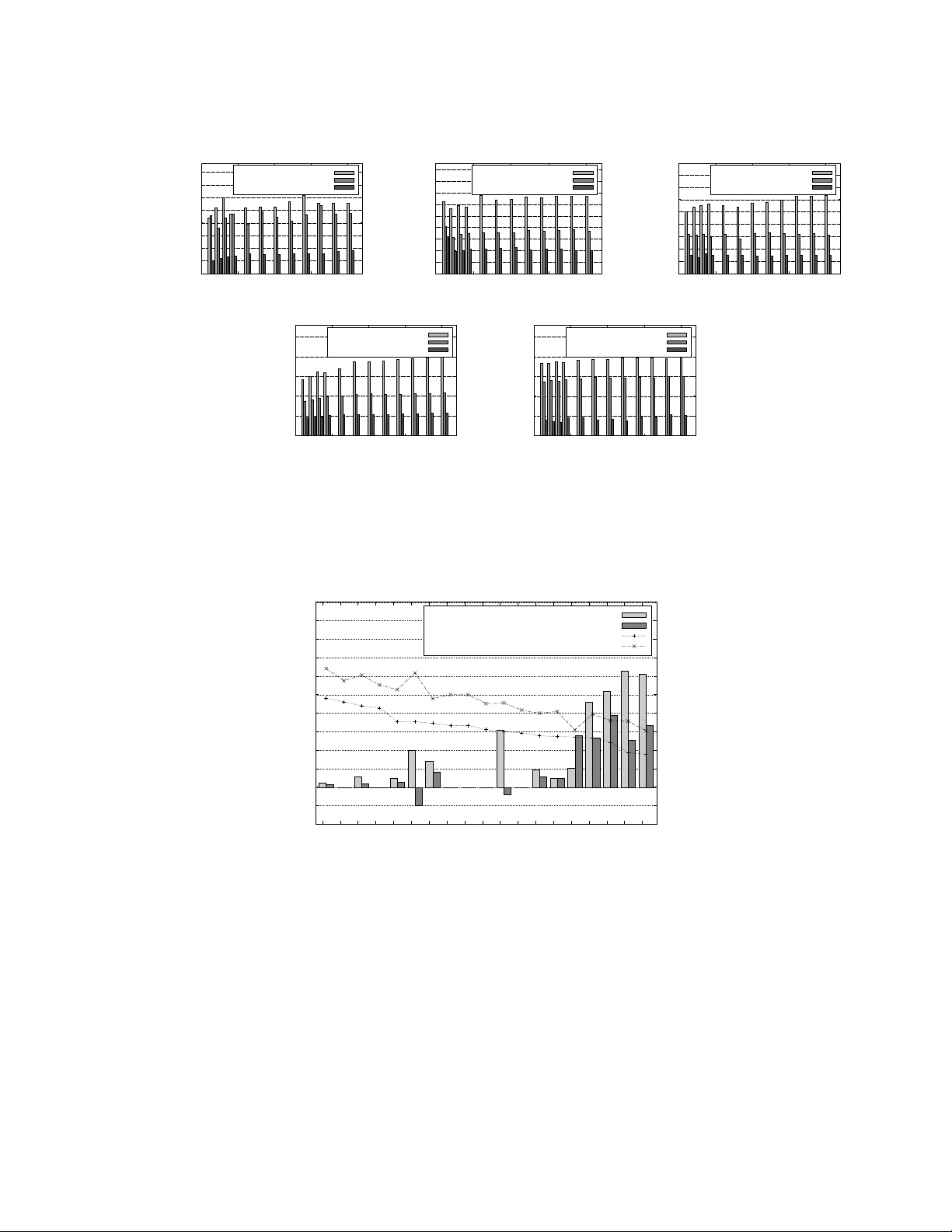
Journal of Artiﬁcial Intelligence Researc h 35 (2009) 449-484 Submitted 1/09; published 7/09 Eﬃcien t Mark o v Net w ork Structure Disco v ery Using Indep endence T ests F acundo Brom b erg fbromber g@frm.utn.edu.ar Dep artamento de Sistemas de Informaci´ on, Universidad T e cnol´ ogic a Nacional, Mendoza, Ar gentina Dimitris Margaritis dmarg@cs.iast a te.edu V asan t Honav ar hona v ar@cs.iast a te.edu Dept. of Computer Scienc e, Iowa State University, A mes, IA 50011 Abstract W e present t wo algorithms for learning the structure of a Marko v netw ork from data: GSMN ∗ and GSIMN. Both algorithms use statistical indep endence tests to infer the struc- ture by successively constraining the set of structures consistent with the results of these tests. Un til very recently , algorithms for structure learning were based on maximum like- liho od estimation, which has b een prov ed to b e NP-hard for Marko v netw orks due to the diﬃcult y of estimating the parameters of the netw ork, needed for the computation of the data lik eliho od. The independence-based approac h do es not require the computation of the likelihoo d, and th us b oth GSMN ∗ and GSIMN can compute the structure eﬃciently (as shown in our exp erimen ts). GSMN ∗ is an adaptation of the Grow-Shrink algorithm of Margaritis and Thrun for learning the structure of Ba yesian net works. GSIMN ex- tends GSMN ∗ b y additionally exploiting Pearl’s well-kno wn prop erties of the conditional indep endence relation to infer nov el independences from known ones, th us a voiding the p er- formance of statistical tests to estimate them. T o accomplish this eﬃciently GSIMN uses the T riangle theorem, also introduced in this work, whic h is a simpliﬁed version of the set of Marko v axioms. Exp erimen tal comparisons on artiﬁcial and real-world data sets show GSIMN can yield signiﬁcant savings with resp ect to GSMN ∗ , while generating a Marko v net work with comparable or in some cases impro ved quality . W e also compare GSIMN to a forward-c haining implementa tion, called GSIMN-FCH, that pro duces all p ossible con- ditional indep endences resulting from rep eatedly applying Pearl’s theorems on the known conditional indep endence tests. The results of this comparison sho w that GSIMN, by the sole use of the T riangle theorem, is nearly optimal in terms of the set of indep endences tests that it infers. 1. In tro duction Graphical mo dels (Bay esian and Marko v netw orks) are an imp ortan t sub class of statisti- cal mo dels that possess adv an tages that include clear seman tics and a sound and widely accepted theoretical foundation (probability theory). Graphical mo dels can b e used to represen t eﬃcien tly the join t probability distribution of a domain. They hav e b een used in n umerous application domains, ranging from discov ering gene expression pathw ays in bioinformatics (F riedman, Linial, Nac hman, & P e’er, 2000) to computer vision (e.g. Geman c  2009 AI Access F oundation. All rights reserved. Bromber g, Margaritis, & Hona v ar Figure 1: Example Marko v netw ork. The nodes represen t v ariables in the domain V = { 0 , 1 , 2 , 3 , 4 , 5 , 6 , 7 } . & Geman, 1984, Besag, Y ork, & Mollie, 1991, Isard, 2003, Anguelo v, T ask ar, Chatalbashev, Koller, Gupta, Heitz, & Ng, 2005). One problem that naturally arises is the construction of suc h models from data (Heck erman, Geiger, & Chick ering, 1995, Buntine, 1994). A solution to this problem, b esides b eing theoretically interesting in itself, also holds the p oten tial of adv ancing the state-of-the-art in application domains where such mo dels are used. In this pap er w e fo cus on the task of learning Marko v netw orks ( MNs ) from data in domains i n which all v ariables are either discrete or contin uous and distributed according to a multidimensional Gaussian distribution. MNs are graphical mo del s that consist of tw o parts: an undirected graph (the mo del structure), and a set of parameters. An example Mark ov netw ork is sho wn in Figure 1. Learning such mo dels from data consists of tw o in- terdep enden t tasks: learning the structure of the netw or k, and, given the learned structure, learning the parameters. In this work we fo cus on the problem of learning the structure of the MN of a domain from data. W e presen t t wo algorithms for MN structure learning from data: GSMN ∗ (Gro w-Shrink Mark ov Netw ork learning algorithm) and GSIMN (Gro w-Shrink Inference-based Mark ov Net work learning algorithm). The GSMN ∗ algorithm is an adaptation to Marko v net works of the GS algorithm by Margaritis and Thrun (2000), originally dev elop ed for learning the structure of B ay esian netw orks. GSMN ∗ w orks b y ﬁrst learning the local neigh b orho o d of each v ariable in the domain (also called the Markov blanket of the v ariable), and then using this information in subsequent steps to improv e eﬃciency . Although in teresting and useful in itself, w e use GSMN ∗ as a p oint of reference of the p erformance with regard to time complexity and accuracy achiev ed by GSIMN, which is the main result of this work. The GSIMN algorithm extends GSMN ∗ b y using P earl’s theorems on the prop erties of the conditional indep endence relation (Pearl, 1988) to infer additional indep endences from a set of indep endences resulting from statistical tests and previous inferences, thus av oiding the execution of these tests on data. This allows savings in execution time and, when data are distributed, communication bandwidth. The rest of the pap er is organized as follo ws: In the next section we presen t previous researc h related to the problem. S ection 3 in tro duces notation, deﬁnitions and presents some in tuition b ehind the t wo algorithms. Section 4 contains the main algorithms, GSMN ∗ and GSIMN, as w ell as concepts and practical details related to their op eration. W e ev aluate GSMN ∗ and GSIMN and presen t our results in Section 5, follo wed by a summary of our 450 Efficient Marko v Network Str ucture Discover y Using Independence Tests w ork and p ossible directions of future researc h in Section 6. Appendices A and B con tain pro ofs of correctness of GSMN ∗ and GSIMN. 2. Related W ork Mark ov net works hav e b een used in the physics and computer vision communities (Geman & Geman, 1984, Besag et al., 1991, Anguelov et al., 2005) where they ha ve b een historically called Mark ov random ﬁelds. Recen tly there has b een interest in their use for spatial data mining, which has applications in geography , transp ortation, agriculture, climatology , ecology and others (Shekhar, Zhang, Huang, & V atsa v ai, 2004). One broad and popular class of algorithms for learning the struct ure of graphical mo dels is the sc or e-b ase d approac h, exempliﬁed for Marko v net works b y Della Pietra, Della Pietra, and Laﬀerty (1997), and McCallum (2003). Score-based approaches conduct a searc h in the space of legal structures in an attempt to discov er a model structure of maxim um score. Due to the intractable size of the searc h space i.e., the space of all legal graphs, whic h is sup er-exponential in size, score-based algorithms m ust usually resort to heuristic search. A t each step of the structure search, a probabilistic inference step is necessary to ev aluate the score (e.g., maxim um lik eliho o d, minimum description length, Lam & Bacch us, 1994, or pseudo-lik eliho o d, Besag, 1974). F or Bay esian netw orks this inference step is tractable and therefore sev eral practical score-based algorithms for structure learning ha v e b een developed (Lam & Bacc hus, 1994, Hec kerman, 1995, Acid & de Campos, 2003). F or Mark ov net w orks ho wev er, probabilistic inference requires the calculation of a normaliz ing constant (also kno wn as partition function), a problem kno wn to b e NP-hard (Jerrum & Sinclair, 1993, Barahona, 1982). A n umber of approaches hav e considered a restricted class of graphical mo dels (e.g. Chow & Liu, 1968, Rebane & P earl, 1989, Srebro & Karger, 2001). Ho wev er, Srebro and Karger (2001) pro ve that ﬁnding the maximum likelihoo d netw ork is NP-hard for Marko v netw orks of tree-width greater than 1. Some w ork in the area of structure learning of undirected graphical mo dels has con- cen trated on the learning of decomposable (also called c hordal) MNs (Srebro & Karger, 2001). An example of learning non-decomp osable MNs is presented in the w ork of Hof- mann and T resp (1998), which is an approach for learning structure in contin uous domains with non-linear relationships among the domain attributes. Their algorithm remov es edges greedily based on a leav e-one-out cross v alidation log-likelihoo d score. A non-score based approac h is in the work of Abb eel, Koller, and Ng (2006), whic h introduces a new class of ef- ﬁcien t algorithms for structure and parameter learning of factor graphs, a class of graphical mo dels that subsumes Marko v and Bay esian net works. Their approac h is based on a new parameterization of the Gibbs distribution in whic h the p oten tial functions are forced to b e probabilit y distributions, and is supp orted by a generalization of the Hammersley-Cliﬀord theorem for factor graphs. It is a promising and theoretically sound approach that ma y lead in the future to practical and eﬃcient algorithms for undirected structure learning. In this w ork w e present algorithms that b elong to the indep endenc e-b ase d or c onstr aint- b ase d approach (Spirtes, Glymour, & Scheines, 2000). Indep endence-based algorithms ex- ploit the fact that a graphical model implies that a set of indep endences exist in the distribu- tion of the domain, and therefore in the data set provided as input to the algorithm (under assumptions, see next section); they w ork by conducting a set of conditional indep endence 451 Bromber g, Margaritis, & Hona v ar tests on data, successively restricting the num b er of p ossible structures consisten t with the results of those tests to a singleton (if p ossible), and inferring that structure as the only p ossible one. A desirable characteristic of indep endence-based approaches is the fact that they do not require the use of probabilistic inference during the discov ery of the structure. Also, such algorithms are amenable to pro ofs of correctness (under assumptions). F or Bay esian netw orks, the indep endence-based approac h has b een mainly exempliﬁed b y the SGS (Spirtes et al ., 2000), PC (Spirtes et al., 2000), and algorithms that learn the Mark ov blanket as a step in learning the B ay esian netw ork structure such as Grow-Shrink (GS) algorithm (Margaritis & Thrun, 2000), IAMB and its v arian ts (Tsamardinos, Aliferis, & Statnik ov, 2003a), HITON-PC and HITON-MB (Aliferis, Tsamardinos, & Statniko v, 2003), MMPC and MMMB (Tsamardinos, Aliferis, & Statniko v, 2003b), and max-min hill clim bing (MMHC) (Tsamardinos, Bro wn, & Ali feris, 2006), all of which are widely used in the ﬁeld. Algorithms for restricted classes such as trees (Chow & Liu, 1968) and p olytrees (Rebane & Pearl, 1989) also exist. F or learning Marko v net works prev ious work has mainly fo cused on learning Gaussian gr aphic al mo dels , where the assumption of a contin uous multiv ariate Gaussian distribution is made; this results in linear dep endences among the v ariables with Gaussian noise (Whit- tak er, 1990, Edward s, 2000). More recent approac hes are included in the works of Dobra, Hans, Jones, Nevins, Y ao, and W est (2004), (Castelo & Rov erato, 2006), Pe˜ na (2008), and Sc h¨ afer and Strimmer (2005), that fo cus on applications of Gaussian graphical mo dels in Bioinformatics. While we do not make the assumption of con tinuous Gaussian v ariables in this pap e r, all algorithms w e presen t are applicable to suc h domains with the use of an appropriate conditional indep endence test (suc h as partial correlation). The GSMN ∗ and GSIMN algorithms presen ted apply to any case where an arbitrary faithful distribu- tion can b e assumed and a probabilistic conditional indep endence test for that distribution is av ailable. The algorithms were ﬁrst introduced by Brom b erg, Margaritis, and Hona v ar (2006); the contributions of the presen t pap er include extending these results b y conducting an extensive ev aluation of their exp erimen tal and theoretical prop erties. More sp eciﬁcally , the contributions include an extensive and systematic exp erimental ev aluation of the pro- p osed algorithms on (a) data sets sampled from artiﬁcially generated netw orks of v arying complexit y and strength of dep endences, as w ell as (b) data sets sampled from net works represen ting real-w orld domains, and (c) formal pro ofs of correctness that guaran tee that the prop osed algorithms will compute the correct Mark ov net work structure of the domain, under the stated assumptions. 3. Notation and Preliminaries W e denote random v ariables with capitals (e.g., X, Y , Z ) and sets of v ariables with b old capitals (e.g., X , Y , Z ). In particular, we denote b y V = { 0 , . . . , n − 1 } the set of all n v ariables in the domain. W e name the v ariables by their indices in V ; for instance, w e refer to the third v ariable in V simply by 3. W e denote the data set as D and its size (n umber of data p oints) b y | D | or N . W e use the notation ( X ⊥ ⊥ Y | Z ) to denote the prop osition that X is indep enden t of Y conditioned on Z , for disjoin t sets of v ariables X , Y , and Z . ( X 6 ⊥ ⊥ Y | Z ) denotes conditional dep endence. W e use ( X ⊥ ⊥ Y | Z ) as shorthand for ( { X }⊥ ⊥{ Y } | Z ) to improv e readability . 452 Efficient Marko v Network Str ucture Discover y Using Independence Tests A Mark ov net work is an undirected graphical mo del that represen ts the joint probabilit y distribution ov er V . Each node in the graph represents one of the random v ariables in the domain, and absences of edges enco de conditional independences among them. W e assume the underlying probabilit y distribution to be gr aph-isomorph (Pearl, 1988) or faithful (Spirtes et al., 2000), which means that it has a faithful undirected graph. A graph G is said to b e faithful to some distribution if its graph connectivity represents exactly those dep endencies and indep endences existen t in the distribution. In detail, this means that that for all disjoint sets X , Y , Z ⊆ V , X is indep endent of Y giv en Z if and only if the set of v ertices Z separates the set of vertices X from the set of vertices Y in the graph G (this is sometimes called the glob al Markov pr op erty , Lauritzen, 1996). In other w ords, this means that, after remo ving all vertices in Z from G (including all edges incident to each of them), there exists no (undirected) path in the remaining graph b et w een an y v ariable in X to some v ariable in Y . F or example, in Figure 1, the set of v ariables { 0 , 5 } separates set { 4 , 6 } from set { 2 } . More generally , it has b een sho wn (P earl, 1988; Theorem 2, page 94 and deﬁnition of graph isomorphism, page 93) that a necessary and suﬃcient condition for a distribution to b e graph-isomorph is for its set of indep endence relations to satisfy the follo wing axioms for all disjoint sets of v ariables X , Y , Z , W and individual v ariable γ : (Symmetry) ( X ⊥ ⊥ Y | Z ) ⇐ ⇒ ( Y ⊥ ⊥ X | Z ) (Decomp osition) ( X ⊥ ⊥ Y ∪ W | Z ) ⇐ ⇒ ( X ⊥ ⊥ Y | Z ) ∧ ( X ⊥ ⊥ W | Z ) (In tersection) ( X ⊥ ⊥ Y | Z ∪ W ) (1) ∧ ( X ⊥ ⊥ W | Z ∪ Y ) = ⇒ ( X ⊥ ⊥ Y ∪ W | Z ) (Strong Union) ( X ⊥ ⊥ Y | Z ) = ⇒ ( X ⊥ ⊥ Y | Z ∪ W ) (T ransitivity) ( X ⊥ ⊥ Y | Z ) = ⇒ ( X ⊥ ⊥ γ | Z ) ∨ ( γ ⊥ ⊥ Y | Z ) F or the op eration of the algorithms we also assume the existence of an oracle that can answ er statistical indep endence queries. These are standard assumptions that are needed for formally proving the correctness of indep endence-based structure learning algorithms (Spirtes et al., 2000). 3.1 Indep endence-Based Approac h to Structure Learning GSMN ∗ and GSIMN are indep endence-based algorithms for learning the structure of the Mark ov net work of a domain. This approach w orks by ev aluating a num b er of statistical indep endence statemen ts, reducing the set of structures consisten t with the results of these tests to a singleton (if p ossible), and inferring that structure as the only p ossible one. As mentioned ab o ve, in theory w e assume the existence of an indep endence-query oracle that can pro vide information about conditional indep endences among the domain v ariables. This can b e viewed as an instance of a statistical query oracle (Kearns & V azirani, 1994). In practice suc h an oracle do es not exist; ho wev er, it can b e implemented approximately b y a statistical test ev aluated on the data set D . F or example, for discrete data this can b e Pearson’s conditional indep endence c hi-square ( χ 2 ) test (Agresti, 2002), a mutual information test etc. F or con tinuous Gaussian data a statistical test that can b e used to measure conditional indep endence is partial correlation (Spirtes et al., 2000). T o determine conditional indep endence b etw een tw o v ariables X and Y given a set Z from data, the 453 Bromber g, Margaritis, & Hona v ar statistical test returns a p-v alue. The p-value of a test equals the probabilit y of obtaining a v alue for the test statistic that is at least as extreme as the one that was actually observed giv en that the nul l hyp othesis is true, which corresp onds to conditional indep endence in our case. Assuming that the p-v alue of a test is p ( X , Y | Z ), the statistical test concludes dep endence if and only if p ( X , Y | Z ) is less than or equal to a threshold α i.e., ( X 6 ⊥ ⊥ Y | Z ) ⇐ ⇒ p ( X , Y | Z ) ≤ α. The quantit y 1 − α is sometimes referred to as the test’s c onﬁdenc e thr eshold . W e use the standard v alue of α = 0 . 05 in all our exp erimen ts, whic h corresp onds to a conﬁdence threshold of 95%. In a faithful domain, it can b e sho wn (Pearl & Paz, 1985) that an edge exists b etw een t wo v ariables X 6 = Y ∈ V in the Mark ov net work of that domain if an only if they are dep enden t conditioned on all remaining v ariables in the domain, i.e., ( X, Y ) is an edge iﬀ ( X 6 ⊥ ⊥ Y | V − { X, Y } ) . Th us, to learn the structure, theoretically it suﬃces to p erform only n ( n − 1) / 2 tests i.e., one test ( X , Y | V − { X, Y } ) for eac h pair of v ariables X , Y ∈ V , X 6 = Y . Unfortunately , in non-trivial domains this usually in volv es a test that conditions on a large n umber of v ariables. Large conditioning sets pro duce sparse con tingency tables (count histograms) whic h result in unreliable tests. This is b ecause the n umber of p ossible conﬁgurations of the v ariables grows exp onen tially with the size of the conditioning set—for example, there are 2 n cells in a test in volving n binary v ariables, and to ﬁll such a table with one data p oin t p er cell we w ould need a data set of at least exp onen tial size i.e., N ≥ 2 n . Exacerbating this problem, more than one data p oin t p er cell is typically necessary for a reliable test: As recommended by Co c hran (1954), if more than 20% of the cells of the contingency table ha ve less than 5 data p oin ts the test is deemed unreliable. Therefore both GSMN ∗ and GSIMN algorithms (presented b elow) attempt to minimize the conditioning set size; they do that by choosing an order of examining the v ariables such that ir rele v ant v ariables are examined last. 4. Algorithms and Related Concepts In this section w e present our main algorithms, GSMN ∗ and GSIMN, and supp orting con- cepts required for their descri ption. F or the purp ose of aiding the understanding of the reader, b efore discussing these w e ﬁrst describ e the abstract GSMN algorithm in the next section. This helps in sho wing the in tuition behind the algorithms and laying the foundation for them. 4.1 The Abstract GSMN Algorithm F or the sake of clarity of exp osition, b efore discussing our ﬁrst algorithm GSMN ∗ , w e describ e the in tuition behind it b y describing its general structure using the abstract GSMN algorithm which delib erately leav es a num b er of details unspeciﬁed; these are ﬁlled-in in the concrete GSMN ∗ algorithm, presented in the next section. Note that the choi ces for these 454 Efficient Marko v Network Str ucture Discover y Using Independence Tests Algorithm 1 GSMN algorithm outline: G = GSMN ( V , D ). 1: I nitialize G to the empty graph. 2: for all v ariables X in the domain V do 3: /* L e arn the Markov Blanket B X of X using the GS algorithm. */ 4: B X ← GS ( X, V , D ) 5: Add an undirected edge in G b etw een X and each v ariable Y ∈ B X . 6: return G Algorithm 2 GS algorithm. Returns the Marko v Blank et B X of v ariable X ∈ V : B X = GS ( X , V , D ). 1: B X ← ∅ 2: / * Gr ow phase. */ 3: for eac h v ariable Y in V − { X } do 4: if ( X 6 ⊥ ⊥ Y | B X ) (estimated using data D ) then 5: B X ← B X ∪ { Y } 6: goto 3 /* R estart gr ow lo op. */ 7: / * Shrink phase. */ 8: for eac h v ariable Y in B X do 9: if ( X ⊥ ⊥ Y | B X − { Y } ) (estimated using data D ) then 10: B X ← B X − { Y } 11: goto 8 /* R estart shrink lo op. */ 12: return B X details are a source of optimizations that can reduce the algorithm’s computational cost. W e make these explicit when we discuss the concrete GSMN ∗ and GSIMN algorithms. The abstract GSMN algorithm is shown in Algorithm 1. Given as input a data set D and a set of v ariables V , GSMN computes the set of no des (v ariables) B X that are adjacen t to each v ariable X ∈ V ; these completely determine the structure of the domain MN. The algorithm consists of a main lo op in which it learns the Marko v blanket B X of each no de (v ariable) X in the domain using the GS algori thm. It then constructs the Marko v net work structure by connecting X with each v ariable in B X . The GS algorithm was ﬁrst prop osed by Margaritis and Thrun (2000) and is shown in Algorithm 2. It consists of tw o phases, a gr ow phase and a shrink phase . The gro w phase of X pro ceeds b y attempting to add each v ariable Y to the curren t set of hypothesized neigh b ors of X , contained in B X , which is i nitially empty . B X gro ws b y some v ariable Y during each iteration of the grow lo op of X if and only if Y is found dep enden t with X giv en the current set of hypothesized neighbors B X . Due to the (unspeciﬁed) ordering that the v ariables are examined (this is explicitly sp eciﬁed in the concrete GSMN ∗ algorithm, presen ted in the next section), at the end of the gro w phase some of the v ariables in B X migh t not b e true neighbors of X in the underlying MN—these ar e called false p ositives . This justiﬁes the shrink phase of the algorithm, whic h remo ves eac h false p ositiv e Y in B X b y testing for indep endence with X conditioned on B X − { Y } . If Y is found independent of X during the shrink phase, it cannot b e a true neighbor (i.e., there cannot be an edge X − Y ), and GSMN remo ves it from B X . Assuming faithfulness and correctness of the indep endence query results, b y the end of the shrink phase B X con tains exactly the neigh b ors of X in the underlying Marko v netw ork. 455 Bromber g, Margaritis, & Hona v ar In the next section w e presen t a concrete implemen tation of GSMN, called GSMN ∗ . This augmen ts GSMN by specifying a concrete ordering that the v ariables X are examined in the main lo op of GSMN (lines 2–5 in Algorithm 1), as well as a concrete order that the v ariables Y are examined in the gro w and shrink phases of the GS algorithm (lines 3–6 and 8–11 in Algorithm 2, resp ectiv ely). 4.2 The Concrete GSMN ∗ Algorithm In this section w e discuss our ﬁrst algorithm, GSMN ∗ (Gro w-Shrink Marko v Netw ork learning algorithm), for learning the structure of the Marko v netw or k of a domain. Note that the reason for in tro ducing GSMN ∗ in addition to our main contribution, the GSIMN algorithm (presen ted later in Section 4.5), is for comparison reasons. In particular, GSIMN and GSMN ∗ ha ve identical structure, following the same order of examination of v ariables, with their only diﬀerence b eing the use of inference b y GSIMN (see details in subsequent sections). Introducing GSMN ∗ therefore makes it possible to measure precisely (through our exp erimen tal results in Section 5) the b eneﬁts of the use of inference on p erformance. The GSMN ∗ algorithm is shown in Algorithm 3. Its structure is similar to the abstract GSMN algorithm. One notable diﬀerence i s that the order that v ariables are examined is no w sp eciﬁed; this is done in the initialization phase where the so-called examination or der π and gr ow or der λ X of eac h v ariable X ∈ V is determined. π and all λ X are priorit y queues and each is initially a p ermutation of V ( λ X is a p erm utation of V − { X } ) suc h that the p osition of a v ariable in the queue denotes its priority e.g., π = [2 , 0 , 1] means that v ariable 2 has the highest priority (will b e examined ﬁrst), follow ed by 0 and ﬁnally b y 1. Similarly , the p osition of a v ariable in λ X determines the order it will b e examined during the grow phase of X . During the initialization phase the algorithm computes the strength of unconditional dep endence b et ween each pair of v ariable X and Y , as giv en by the unconditional p-v alue p ( X, Y | ∅ ) of an indep endence test b et ween each pair of v ariables X 6 = Y , denoted by p X Y in the algorithm. (In practice the logarithm of the p-v alues is computed, which allo ws greater precision in domains where some dep endencies may b e very strong or very w eak.) In particular, the algorithm gives higher priority to (examines earlier) those v ariables with a lo wer av erage log p-v alue (line 5), indicating stronger dep endence. This av erage is deﬁned as: a vg Y log( p X Y ) = 1 | V | − 1 X Y 6 = X log( p X Y ) . F or the grow order λ X of v ariable X , the algorithm gives higher priority to those v ariables Y whose p-v alue (or equiv alently the l og of the p-v alue) with v ariable X is small (line 8). This ordering is due to the intuition b ehind the “folk-theorem” (as Koller & Sahami, 1996, puts it) that states that probabilistic inﬂuence or asso ciation b et w een attributes tends to atten uate ov er distance in a graphical mo del. This suggests that a pair of v ariables X and Y with high unconditional p-v alue are less likely to b e directly link ed. Note that this ordering is a heuristic and is not guaranteed to hold in general. F or example, it ma y not hold if the underlying domain is a Bay esian net work e.g., tw o “sp ouses” may b e indep endent unconditionally but dep enden t conditional on a common child. Note how ever that this example do es not apply to faithful domains i.e., graph-isomorph to a Marko v net work. Also 456 Efficient Marko v Network Str ucture Discover y Using Independence Tests Algorithm 3 GSMN ∗ , a concrete implemen tation of GSMN: G = GSMN ∗ ( V , D ). 1: I nitialize G to the empty graph. 2: / * Initialization. */ 3: for all X , Y ∈ V , X 6 = Y do 4: p X Y ← p ( X, Y | ∅ ) 5: I nitialize π such that ∀ i, i ′ ∈ { 0 , . . . , n − 1 } ,  i < i ′ ⇐ ⇒ avg j log( p π i j ) < a vg j log( p π i ′ j )  . 6: for all X ∈ V do 7: B X ← ∅ 8: Initialize λ X suc h that ∀ j, j ′ ∈ { 0 , . . . , n − 1 } ,  j < j ′ ⇐ ⇒ p X λ X j < p X λ X j ′  . 9: Remo ve X from λ X . 10: / * Main lo op. */ 11: while π is not empty do 12: X ← deq ueue ( π ) 13: /* Pr op agation phase. */ 14: T ← { Y : Y was examined and X ∈ B Y } 15: F ← { Y : Y was examined and X / ∈ B Y } 16: for all Y ∈ T , mo ve Y to the end of λ X . 17: for all Y ∈ F , mo ve Y to the end of λ X . 18: /* Gr ow phase. */ 19: S ← ∅ 20: while λ X not empt y do 21: Y ← deq ueue ( λ X ) 22: if p X Y ≤ α then 23: if ¬ I GSMN ∗ ( X, Y , S , F , T ) then 24: S ← S ∪ { Y } 25: /* Change gr ow or der of Y . */ 26: Mo ve X to the b eginning of λ Y . 27: for W = S | S |− 2 to S 0 do 28: Mo ve W to the b eginning of λ Y . 29: /* Change examination or der. */ 30: for W = S | S |− 1 to S 0 do 31: if W ∈ π then 32: Mo ve W to the b eginning of π . 33: break to line 34 34: /* Shrink phase. */ 35: for Y = S | S |− 1 to S 0 do 36: if I GSMN ∗ ( X, Y , S − { Y } , F , T ) then 37: S ← S − { Y } 38: B X ← S 39: Add an undirected edge in G b etw een X and each v ariable Y ∈ B X . 40: return G note that the correctness of all algorithms we present do es not dep end on it holding i.e., as we pro ve in App endices A and B, b oth GSMN ∗ and GSIMN are guaranteed to return the correct structure under the assumptions stated in Section 3 ab ov e. Also note that the computational cost for the calculation of p X Y is low due to the empty conditioning set. The remaining of the GSMN ∗ algorithm con tains the main lo op (lines 10–39) in which eac h v ariable in V is examined according to the examination order π , determined during 457 Bromber g, Margaritis, & Hona v ar Algorithm 4 I GSMN ∗ ( X, Y , S , F , T ): Calculate indep endence test ( X , Y | S ) by propaga- tion, if p ossible, otherwise run a statistical test on data. 1: / * Attempt to infer dep endenc e by pr op agation. */ 2: i f Y ∈ T then 3: return false 4: / * Attempt to infer indep endenc e by pr op agation. */ 5: i f Y ∈ F then 6: return true 7: / * Else do statistic al test on data. */ 8: t ← 1 ( p ( X,Y | Z ) >α ) /* t = true iﬀ p-value of statistic al test ( X , Y | S ) > α . */ 9: return t the initialization phase. The main lo op includes three phases: the pr op agation phase (lines 13–17), the gr ow phase (lines 18–33), and the shrink phase (lines 34–37). The propagation phase is an optimization in whic h all v ariables Y for which B Y has already b een computed (i.e., all v ariables Y already examined) are collected in tw o sets F and T . Set F ( T ) contains all v ariables Y such that X / ∈ B Y ( X ∈ B Y ). Both sets are passed to the indep endence pro cedure I GSMN ∗ , shown in Algorithm 4, for the purp ose of a voiding the execution of any tests b etw een X and Y by the algorithm. This is justiﬁed by the fact that, in undirected graphs, Y is in the Marko v blank et of X if and only if X is in the Marko v blank et of Y . V ariables Y already found not to con tain X in their blanket B Y (set F ) cannot b e mem b ers of B X b ecause there exi sts some set of v ariables that has rendered them conditionally indep enden t of X in a previous step, and indep endence can therefore b e inferred easily . Note that in the exp erimen ts section of the pap er (Section 5) we ev aluate GSMN ∗ with and without the propagation phase, in order to measure the eﬀect that this propagation optimization has on p erformance. T urning oﬀ propagation i s accomplished simply b y setting sets T and F (as computed in lines 14 and 15, resp ectiv ely) to the empty set. Another diﬀerence of GSMN ∗ from the abstract GSMN algorithm is in the use of condi- tion p X Y ≤ α (line 22). This is an additional optimization that av oids an indep endence test in the case that X and Y w ere found (unconditionally) independent during the initialization phase, since in that c ase this would imply X and Y are indep enden t given any conditioning set by the axiom of Strong Union. A crucial diﬀerence betw een GSMN ∗ and the abstract GSMN algori thm is that GSMN ∗ c hanges the examination order π and the grow order λ Y of every v ariable Y ∈ λ X . (Since X / ∈ λ X , this excludes the grow order of X itself.) These changes in ordering pro ceed as follo ws: After the end of the grow phase of v ariable X , the new examination order π (set in lines 30–33) dictates that the next v ariable W to b e examined after X is the last to b e added to S during the growing phase that has not yet b een examined (i.e., W is still in π ). The grow order λ Y of all v ariables Y found dep enden t with X is also c hanged; this is done to maximize the num b er of optimizations by the GSIMN algorithm (our main contribution in this pap er) which shares the algorithm structure of GSMN ∗ . The changes in grow order are therefore explained in detail in Section 4.5 when GSIMN is presented. A ﬁnal diﬀerence b etw een GSMN ∗ and the abstract GSMN algorithm is the restart actions of the grow and shrink phases of GSMN whenever the current Marko v blanket is mo diﬁed (lines 6 and 11 of Algorithm 2), which are not present in GSMN ∗ . The restarting 458 Efficient Marko v Network Str ucture Discover y Using Independence Tests Figure 2: Illustration of the op eration of GSMN ∗ using an indep endence graph. The ﬁgure sho ws the growing phase of v ariable 5. V ariables are examined according to its gro w order λ 5 = [3 , 4 , 1 , 6 , 2 , 7 , 0]. of the lo ops w as necessary in the GS algorithm due to its original usage in learning the structure of Bay esian netw orks. In that task, it was p ossible for a true mem b er Y of the blank et of X to b e found initially indep enden t during the grow lo op when conditioning on some set S but to b e found dep enden t later when conditioned on a sup erset S ′ ⊃ S . This could happ en i f Y was an “unshielded sp ouse” of X i.e., if Y had one or more common c hildren with X but there existed no direct link b etw een Y and X in the underlying Ba yesian net work. How ever, this b eha vior is imp ossible in a domain that has a distribution faithful to a Marko v netw ork (one of our assumptions): an y indep endence b et ween X and Y given S must hold for an y superset S ′ of S by the axiom of Strong Union (see Eqs. (1)). The restart of the gro w and shrink lo ops is therefore omitted from GSMN ∗ in order to sa ve unnecessary tests. Note that, even though it is p ossible that this b eha vior is imp ossible in faithful domains, it is p ossible in unfaithful ones, so we also exp erimen tally ev aluated our algorithms in real-world domains in which the assumption of Marko v faithfulness may not necessarily hold (Section 5). A pro of of correctness of GSMN ∗ is presented in App endix A. 4.3 Indep endence Graphs W e can demonstrate the op eration of GSMN ∗ graphically by the concept of the indep endenc e gr aph , whic h w e no w in tro duce. W e deﬁne an indep endence graph to b e an undirected graph in which conditional independences and dependencies b et ween single v ariables are represen ted by one or more annotate d e dges b et ween them. A solid (dotted) edge b et ween v ariables X and Y annotated by Z represen ts the fact that X and Y hav e b een found dep enden t (indep endent) giv en Z . If the conditioning set Z is enclosed in parentheses then this edge represents an indep endence or dep endence that w as inferr e d from Eqs. (1) (as opp osed to computed from statistical tests). Sho wn graphically: 459 Bromber g, Margaritis, & Hona v ar X Y Z ( X 6 ⊥ ⊥ Y | Z ) X Y Z ( X ⊥ ⊥ Y | Z ) X Y (Z) ( X 6 ⊥ ⊥ Y | Z ) (inferred) X Y (Z) ( X ⊥ ⊥ Y | Z ) (inferred) F or instance, in Figure 2, the dotted edge b et ween 5 and 1 annotated with “3 , 4” represen ts the fact that (5 ⊥ ⊥ 1 | { 3 , 4 } ). The absence of an edge b et ween tw o v ariables indicates the absence of information ab out the independence or dep endence b et ween these v ariables under an y conditioning set. Example 1. Figur e 2 il lust r ates the op er atio n of GSMN ∗ using an indep endenc e gr aph in the domain whose underlying Markov network is shown in Figur e 1. The ﬁgur e shows the indep endenc e gr aph at the end of the gr ow phase of the variable 5 , the ﬁrst in the examination or der π . (We do not discuss in this example the initialization phase of GSMN ∗ ; inste ad, we assume that the examination ( π ) and gr ow ( λ ) or ders ar e as shown in the ﬁgur e.) A c c or ding to vertex sep ar ation on the underlying network (Figur e 1), variables 3 , 4 , 6 , and 7 ar e found dep endent with 5 during the gr owing phase i.e., ¬ I (5 , 3 | ∅ ) , ¬ I (5 , 4 | { 3 } ) , ¬ I (5 , 6 | { 3 , 4 } ) , ¬ I (5 , 7 | { 3 , 4 , 6 } ) and ar e ther efor e c onne cte d to 5 i n the indep endenc e gr aph by solid e dges annotate d by sets ∅ , { 3 } , { 3 , 4 } and { 3 , 4 , 6 } r esp e ctively. V ariables 1 , 2 , and 0 ar e found indep endent i.e., I (5 , 1 | { 3 , 4 } ) , I (5 , 2 | { 3 , 4 , 6 } ) , I (5 , 0 | { 3 , 4 , 6 , 7 } ) and ar e thus c onne cte d to 5 by dotte d e dges annotate d by { 3 , 4 } , { 3 , 4 , 6 } and { 3 , 4 , 6 , 7 } r esp e ctively. 4.4 The T riangle Theorem In this section we present and prov e a theorem that is used in the subsequent GSIMN algorithm. As will b e seen, the main idea behind the GSIMN algorithm is to attempt to de- crease the num b er of tests done by exploiting the prop erties of the conditional indep endence relation in faithful domains i.e., Eqs. (1). These prop erties can b e seen as inference rules that can b e used to deriv e new indep endences from ones that w e kno w to b e true. A careful study of these axioms suggests that only tw o simple inference rules, stated in the T riangle the or em b elo w, are suﬃcien t for inferring most of the useful indep endence information that can b e inferred by a systematic application of the inference r ules. This is conﬁrmed in our exp erimen ts in Section 5. 460 Efficient Marko v Network Str ucture Discover y Using Independence Tests Figure 3: Indep endence graph depicting the T riangle theorem. Edges in the graph are lab eled b y sets and represen t conditional independences or dep endencies. A solid (dotted) edge b et w een X and Y lab eled by Z means that X and Y are dep enden t (indep enden t) giv en Z . A set lab el enclosed in parentheses means the e dge was inferred by the theorem. Theorem 1 (T riangle theorem) . Given Eqs. (1), for every variable X , Y , W and sets Z 1 and Z 2 such that { X , Y , W } ∩ Z 1 = { X , Y , W } ∩ Z 2 = ∅ , ( X 6 ⊥ ⊥ W | Z 1 ) ∧ ( W 6 ⊥ ⊥ Y | Z 2 ) = ⇒ ( X 6 ⊥ ⊥ Y | Z 1 ∩ Z 2 ) ( X ⊥ ⊥ W | Z 1 ) ∧ ( W 6 ⊥ ⊥ Y | Z 1 ∪ Z 2 ) = ⇒ ( X ⊥ ⊥ Y | Z 1 ) . We c al l the ﬁrst r elation the “D-triangle rul e” and the se c ond the “I-triangle rule.” Pr o of. W e are using the Strong Union and T ransitivity of Eqs. (1) as shown or in contra- p ositiv e form. (Pro of of D-triangle rule) : • F rom Strong Union and ( X 6 ⊥ ⊥ W | Z 1 ) we get ( X 6 ⊥ ⊥ W | Z 1 ∩ Z 2 ). • F rom Strong Union and ( W 6 ⊥ ⊥ Y | Z 1 ) we get ( W 6 ⊥ ⊥ Y | Z 1 ∩ Z 2 ). • F rom T r ansitivity , ( X 6 ⊥ ⊥ W | Z 1 ∩ Z 2 ), and ( W 6 ⊥ ⊥ Y | Z 1 ∩ Z 2 ), we get ( X 6 ⊥ ⊥ Y | Z 1 ∩ Z 2 ). (Pro of of I-triangle rule) : • F rom Strong Union and ( W 6 ⊥ ⊥ Y | Z 1 ∪ Z 2 ) we get ( W 6 ⊥ ⊥ Y | Z 1 ). • F rom T ransitivity , ( X ⊥ ⊥ W | Z 1 ) and ( W 6 ⊥ ⊥ Y | Z 1 ) we get ( X ⊥ ⊥ Y | Z 1 ). W e can represent the T riangle theorem gr aphically using the indep endence graph con- struct of Section 4.2. Figure 3 depicts the t wo rules of the T riangle theorem using tw o indep endence graphs. The T riangle theorem can b e used to infer additional conditional indep endences from tests conducted during the op eration of GSMN ∗ . An example of this is shown in Fig- ure 4, which illustrates the application of the T riangle theorem to the example presented in Figure 2. The indep endence information inferred from the T riangle theorem is shown b y curv ed edges (note that the conditioning set of eac h such edge is enclosed in paren theses). 461 Bromber g, Margaritis, & Hona v ar Figure 4: Illustration of the use of the T riangle theorem on the example of Figure 2. The set of v ariables enclosed in paren theses corresp ond to tests inferred by the T riangle theorem using the tw o adjacent edges as an teceden ts. F or example, the result (1 ⊥ ⊥ 7 | { 3 , 4 } ), is inferred from the I-triangle rule, indep endence (5 ⊥ ⊥ 1 | { 3 , 4 } ) and dep endence (5 6 ⊥ ⊥ 7 | { 3 , 4 , 6 } ). F or example, indep endence edge (4 , 7) can b e inferred b y the D-triangle rule from the ad- jacen t edges (5 , 4) and (5 , 7), annotated b y { 3 } and { 3 , 4 , 6 } resp ectiv ely . The annotation for this inferred edge is { 3 } , which is the intersection of the annotations { 3 } and { 3 , 4 , 6 } . An example application of the I-triangle rule is edge (1 , 7), which is inferred from edges (5 , 1) and (5 , 7) with annotations { 3 , 4 } and { 3 , 4 , 6 } resp ectiv ely . The annotation for this inferred edge is { 3 , 4 } , which is the intersection of the annotations { 3 , 4 , 6 } and { 3 , 4 } . 4.5 The GSIMN Algorithm In the previous section we sa w the p ossibilit y of using the tw o rules of the T riangle theorem to infer the result of nov el tests during the gro w phase. The GSIMN algorithm (Gro w-Shrink Inference-based Marko v Netw ork learning algorithm), introduced in this sec- tion, uses the T riangle theorem in a similar fashion to extend GSMN ∗ b y inferring the v alue of a n umber of tests that GSMN ∗ executes, making their ev aluation unnecessary . GSIMN and GSMN ∗ w ork in exactly the same wa y (and thus the GSIMN algorithm shares exactly the same algorithmic description i.e., both follo w Algorithm 3), with all diﬀerences b etw een them concentrat ed in the indep endence pro cedure they use: instead of using indep endence pro cedure I GSMN ∗ of GSMN ∗ , GSIMN uses pro cedure I GSIMN , sho wn in Algorithm 5. Pro- cedure I GSIMN , in addition to attempting to propagate the blanket information obtained from the examination of previous v ariables (as I GSMN ∗ do es), also attempts to infer the v alue of the indep endence test that is provided as its input b y either the Strong Union axiom (listed in Eqs. (1)) or the T riangle theorem. If this attempt is successful, I GSIMN returns the v alue inferred ( true or false ), otherwise it defaults to a statistical test on the data set (as I GSMN ∗ do es). F or the purp ose of assisting in the inference pro cess, GSIMN and 462 Efficient Marko v Network Str ucture Discover y Using Independence Tests Algorithm 5 I GSIMN ( X, Y , S , F , T ): Calculate indep endence test result by inference (in- cluding propagation), if p ossible. Record test result in the kno wledge base. 1: / * Attempt to infer dep endenc e by pr op agation. */ 2: i f Y ∈ T then 3: return false 4: / * Attempt to infer indep endenc e by pr op agation. */ 5: i f Y ∈ F then 6: return true 7: / * Attempt to infer dep endenc e by Str ong Union. */ 8: i f ∃ ( A , false ) ∈ K X Y suc h that A ⊇ S then 9: return false 10: / * Attempt to infer dep endenc e by the D-triangle rule. */ 11: for all W ∈ S do 12: if ∃ ( A , false ) ∈ K X W suc h that A ⊇ S ∧ ∃ ( B , false ) ∈ K W Y suc h that B ⊇ S then 13: Add ( A ∩ B , false ) to K X Y and K Y X . 14: return false 15: / * Attempt to infer indep endenc e by Str ong Union. */ 16: i f ∃ ( A , true ) ∈ K X Y suc h that A ⊆ S then 17: return true 18: / * Attempt to infer indep endenc e by the I-triangle rule. */ 19: for all W ∈ S do 20: if ∃ ( A , true ) ∈ K X W s.t. A ⊆ S ∧ ∃ ( B , false ) ∈ K W Y s.t. B ⊇ A then 21: Add ( A , true ) to K X Y and K Y X . 22: return true 23: / * Else do statistic al test on data. */ 24: t ← 1 ( p ( X,Y | Z ) >α ) /* t = true iﬀ p-value of statistic al test ( X , Y | S ) > α . */ 25: Add ( S, t ) to K X Y and K Y X . 26: return t I GSIMN main tain a knowledge base K X Y for eac h pair of v ariables X and Y , containing the outcomes of all tests ev aluated so far b et w een X and Y (either from data or inferred). Eac h of these kno wledge bases is empt y at the b eginning of the GSIMN algorithm (the initializa- tion step is not shown in the algorithm since GSMN ∗ do es not use it), and i s main tained within the test pro cedure I GSIMN . W e now explain I GSIMN (Algorithm 5) in detail. I GSIMN attempts to infer the in- dep endence v alue of its input triplet ( X, Y | S ) by applying a single step of backw ard c haining using the Strong Union and T riangle r ules i.e., it searc hes the knowledge base K = { K X Y : X , Y ∈ V } for anteceden ts of instances of rules that hav e the input triplet ( X, Y | S ) as consequent. The Strong Union rule is used in its direct from as sho wn in Eqs. (1) and also in its con trap ositive form. The direct form can b e used to i nfer indep en- dences, and therefore we refer to it as the I-SU rule from here on. In its con trap ositiv e form, the I-SU rule b ecomes ( X 6 ⊥ ⊥ Y | S ∪ W ) = ⇒ ( X 6 ⊥ ⊥ Y | S ), referred to as the D-SU rule since i t can b e used to infer dep endencies. According to the D-T riangle and D-SU rules, the dep endence ( X 6 ⊥ ⊥ Y | S ) can b e inferred if the knowledge base K contains 1. a test ( X 6 ⊥ ⊥ Y | A ) with A ⊇ S , or 2. tests ( X 6 ⊥ ⊥ W | A ) and ( W 6 ⊥ ⊥ Y | B ) for some v ariable W , with A ⊇ S and B ⊇ S , 463 Bromber g, Margaritis, & Hona v ar Figure 5: Illustration of the op eration of GSIMN. The ﬁgure sho ws the grow phase of tw o consecutiv ely examined v ariables 5 and 7. The ﬁgure shows ho w the v ariable examined se cond is not 3 but 7, according to the c hange in the examination order π in lines 30–33 of Algorithm 3. The set of v ariables enclosed in parentheses corresp ond to tests inferred by the T riangle theorem using t wo adjacen t edges as an tecedents. The results (7 6 ⊥ ⊥ 3 | ∅ ), (7 6 ⊥ ⊥ 4 | { 3 } ), (7 6 ⊥ ⊥ 6 | { 3 , 4 } ), and (7 6 ⊥ ⊥ 5 | { 3 , 4 , 6 } ) in (b), sho wn highlighted, w ere not executed but inferred f rom the tests done in (a). resp ectiv ely . According to the I-T riangle and I-SU rules, the indep endence ( X ⊥ ⊥ Y | S ) can b e inferred if the kno wledge base contains 3. a test ( X ⊥ ⊥ Y | A ) with A ⊆ S , or 4. tests ( X ⊥ ⊥ W | A ) and ( W 6 ⊥ ⊥ Y | B ) for some v ariable W , with A ⊆ S and B ⊇ A , resp ectiv ely . The changes to the grow orders of some v ariables o ccur inside the gro w phase of the curren tly examined v ariable X (lines 25–28 of GSIMN i.e., Algorithm 3 with I GSMN ∗ re- placed b y I GSIMN .). In particular, if, for some v ariable Y , the algorithm reaches line 24, i.e., p X Y ≤ α and I GSIMN ( X, Y , S ) = false , then X and all the v ariables that were found dep enden t with X b efore Y (i.e., all v ariables currently in S ) are promoted to the b eginning of the gr ow order λ Y . This is illustrated in Figure 5 for v ariable 7, which depicts the grow phase of t w o consecutively examined v ariables 5 and 7. In this ﬁgure, the curv ed edges sho w the tests that are inferred b y I GSIMN during the grow phase of v ariable 5. The grow order of 7 changes from λ 7 = [2 , 6 , 3 , 0 , 4 , 1 , 5] to λ 7 = [3 , 4 , 6 , 5 , 2 , 0 , 1] after the grow phase of v ariable 5 is complete b ecause the v ariables 5, 6, 4 and 3 w ere promoted (in that order) to the b eginning of the queue. The rationale for this is the observ ation that this increases the n umber of tests inferred b y GSIMN at the next step: The change in the examination and grow orders describ ed ab o v e was chosen so that the inferred tests while learning the blank et of v ariable 7 match exactly those required by the algorithm in some future step. In 464 Efficient Marko v Network Str ucture Discover y Using Independence Tests particular, note that in the example the set of inferred dep endencies b et ween each v ariable found dep endent with 5 b efore 7 are exactly those required during initial part of the grow phase of v ariable 7, shown highligh ted in Figure 5(b) (the ﬁrst four dep endencies). These indep endence tests were inferred (not conducted), resulting in computational savings. In general, the last dep enden t v ariable of the grow phase of X has the maxim um num b er of dep endences and indep endences inferred and this pro vides the rationale for its change in gro w order and its selection by the algorithm to b e examined next. It can b e sho wn that under the same assumptions as GSMN ∗ , the structure returned b y GSIMN is the correct one i.e., each set B X computed by the GSIMN algorithm equals exactly the neigh b ors of X . The pro of of correctness of GSIMN is based on correctness of GSMN ∗ and is presented i n App endix B. 4.6 GSIMN T echnical Implemen tation Details In this section w e discuss a num b er of practical issues that subtly inﬂuence the accuracy and eﬃciency of an implementation of GSIMN. One is the order of application of the I-SU, D-SU, I-T riangle and D-T riangle rules within the function I GSIMN . Given an indep endence-query oracle, the order of application should not matter—assuming there are more than one rules for inferring the v al ue of an indep endence, all of them are guaranteed to pro duce the same v alue due to the soundness of the axioms of Eqs. (1) (Pearl, 1988). In practice ho w ever, the oracle is implemented by statistical tests conducted on data whic h c an b e incorrect, as previously men tioned. Of particular imp ortance is the observ ation that false indep endences are more likely to o ccur than false dep endencies. One example of this is the case where the domain dep endencies are w eak—in this case an y pair of v ariables connected (dep enden t) in the underlying true netw ork structure may b e incorrectly deemed indep endent if all paths b et w een them are long enough. On the other hand, false dep endencies are m uch more rare— the conﬁdence threshold of 1 − α = 0 . 95 of a statistical test tells us that the probabilit y of a false dep endence by c hance alone is only 5%. Assuming i.i.d. data for each test, the chance of multiple false dep endencies is even low er, decreasing exp onentially fast. This practical observ ation i.e., that dep endencies are typically more reliable than indep endences, provide the rationale for the wa y the I GSIMN algorithm works. In particular, I GSIMN prioritizes the application of rules whose anteceden ts con tain dep endencies ﬁrst i.e., the D-T riangle and D-SU rules, follo wed by the I-T riangle and I-SU rules. In eﬀect, this uses statistical results that are typically kno wn with greater conﬁdence b efore ones that are usually less reliable. The second practical issue concerns eﬃcien t inference. The GSIMN algorithm uses a one- step inference pro cedure (sho wn in Algorithm 5) that utilizes a kno wledge base K = { K X Y } con taining known indep endences and dep endences for eac h pair of v ariables X and Y . T o implemen t this inference eﬃciently w e utilize a data structure for K for the purp ose of storing and retrieving indep endence facts in constant time. It consists of tw o 2D arrays, one for dep endencies and another for indep endencies. Each array is of n × n size, where n is the num b er of v ariables in the domain. Each cell in this array corresp onds to a pair of v ariables ( X , Y ), and stores the known indep endences (dep endences) b et ween X and Y in the form of a list of conditioning sets. F or eac h conditioning set Z in the list, the kno wledge base K X Y represen ts a kno wn indep endence ( X ⊥ ⊥ Y | Z ) (dep endence ( X 6 ⊥ ⊥ Y | Z )). It i s imp ortan t to note that the length of each list is at most 2, as there are no more than tw o 465 Bromber g, Margaritis, & Hona v ar tests done b et ween any v ariable X and Y during the execution of GSIMN (done during the growing and shrinking phases). Th us, it alwa ys takes a constan t time to retrieve/store an indep endence (dep endence), and therefore all inferences using the knowledge base are constan t time as w ell. Also note that all uses of the Strong Union axion by the I GSIMN algorithm are constan t time as w ell, as they can b e accomplished b y testing the (at most t wo) sets stored in K X Y for subset or sup erset inclusion. 5. Exp erimen tal Results W e ev aluated the GSMN ∗ and GSIMN algorithms on b oth artiﬁcial and real-world data sets. Through the exp erimen tal results pre sented b elo w we show that the simple application of P earl’s inference rules in GSIMN algorithm results in a signiﬁcan t reduction in the num b er of tests p erformed when compared to GSMN ∗ without adv ersely aﬀecting the quality of the output netw ork. In particular we rep ort the following quant ities: • W eigh ted n um b er of tests. The w eighted n umber of tests is computed b y the summation of the weigh t of each test executed, where the weight of test ( X , Y | Z ) is deﬁned as 2 + | Z | . This quan tit y reﬂects the time complexity of the algorithm (GSMN ∗ or GSIMN) and can be used to assess the b eneﬁt in GSIMN of using inference instead of executing statistical tests on data. This is the standard metho d of comparison of indep endence-based algorithms and it is justiﬁed by the observ ation that the running time of a statistical test on triplet ( X , Y | Z ) is prop ortional to the size N of the data set and the n umber of v ariables in volv ed in it i.e., O ( N ( | Z | + 2)) (and is not exp onential in the num b er of v ariables inv olved as a na ¨ ıv e implementation might assume). This is b ecause one can construct all non-zero entries in the con tingency table used by the test by examining eac h data point in the data set exactly once, in time prop ortional to the num b er of v ariables inv olved in the test i.e., prop ortional to |{ X , Y } ∪ Z | = 2 + | Z | . • Execution time. In order to assess the impact of inference in the running time (in addition to the impact of statistical tests), we rep ort the execution time of the algorithm. • Qualit y of the resulting netw ork. W e measure quality in t wo wa ys. – Normalized Hamming distance. The Hamming distance betw een the output net work and the structure of the underlying mo del is another measure of the qualit y of the output netw ork, when the actual net work that w as used to generate the data is kno wn. The Hamming distance is deﬁned as the num b er of “rev ersed” edges b et ween these tw o netw ork structures, i.e., the n umber of times an actual edge in the true netw ork is missing in the returned netw ork or an edge absent from the true net work exists in the algorithm’s output net work. A v alue zero means that the output netw ork has the correct structure. T o be able to compare domains of diﬀerent dimensionalities (n umber of v ariables n ) we normalize it by  n 2  , the total n umber of no de pairs in the corresp onding domain. – Accuracy . F or real-world data sets where the underlying netw ork is unkno wn, no Hamming distance calculation is p ossible. In this case it is imp ossible to know the true v alue of any independence. W e therefore approximate it b y a statistical test on the entire data set, and use a limited, randomly chosen subset (1/3 of the data set) to learn the netw ork. T o measure accuracy we compare the result 466 Efficient Marko v Network Str ucture Discover y Using Independence Tests ( true or false ) of a n umber of conditional indep endence tests on the net work output (using vertex separation), to the same tests p erformed on the full data set. In all exp eriments inv olving data sets we used the χ 2 statistical test for estimation of conditional independences. As mentioned ab o ve, rules of th umb exist that deem certain tests as p oten tially unreliable dep ending on the coun ts of the contingency table inv olved; for example, one such rule Co c hran (1954) deems a test unreliable if more than 20% of the cells of the con tingency table hav e less than 5 data p oints the test. Due to the requiremen t that an answer m ust b e obtained by an indep endence algorithm conducting a test, we used the outcomes of suc h tests as w ell in our exp erimen ts. The eﬀect of these possibly unreliable tests on the qualit y of the resulting net work is measured by our accuracy measures, listed ab o v e. In the next section we presen t results for domains in whic h the underlying probabilistic mo del is known. This is follow ed by real-w orld data exp erimen ts where no mo del structure is av ailable. 5.1 Kno wn-Mo del Exp erimen ts In the ﬁrst set of experiments the underlying model, called the true mo del or true network , is a kno wn Mark ov netw ork. The purp ose of this set of experiments is to conduct a con trolled ev aluation of the qualit y of the output netw ork through a systematic study of the algorithms’ b eha vior under v arying conditions of domain size (n umber of v ariables) and amount of dep endencies (av erage no de degree in the netw ork). Eac h true net work that contains n v ariables was generated randomly as follo ws: the net work was initialized with n no des and no edges. A user-sp eciﬁed parameter of the net work structure is the av erage no de degree τ that equals the av erage n um b er of neighbors p er no de. Given τ , for every no de its set of neighbors w as determined randomly and uniformly b y selecting the ﬁrst τ n 2 pairs in a random p erm utation of all p ossible pairs. The factor 1 / 2 is necessary b ecause each edge con tributes to the degree of tw o no des. W e conducted t wo t yp es of exp erimen ts using kno wn net work structure: Exact le arning exp erimen ts and sample-b ase d exp erimen ts. 5.1.1 Exact Learning Experiments In this set of kno wn-mo del exp erimen ts, w e assume that the result of all statistical queries ask ed b y the GSMN ∗ and GSIMN algorithms were a v ailable, whic h assumes the existence of an oracle that can answ er indep endence queries. When the underlying mo del is known, this oracl e can be implemented through v ertex separation. The b eneﬁts of querying the true netw ork for indep endence are tw o: First, it ensures faithfulness and correctness of the indep endence query results, which allo ws the ev aluation of the algorithms under their assumptions for c orrectness. Second, these tests can b e p erformed m uch faster than actual statistical tests on data. This allow ed us to ev aluate our algorithms in large net works—w e w ere able to conduct exp erimen ts of domains containing up to 100 v ariables. W e ﬁrst rep ort the w eighted num b er of tests executed b y GSMN ∗ with and without propagation and GSIMN. Our results are summarized in Figure 6, whic h shows the ratio b et w een the w eighted num b er of tests of GSIMN and the t wo versions of GSMN ∗ . One 467 Bromber g, Margaritis, & Hona v ar 0 0.1 0.2 0.3 0.4 0.5 0.6 0.7 0.8 0.9 1 0 10 20 30 40 50 60 70 80 90 100 WC(GSIMN) / WC(GSMN* with propagation) Domain size (number of variables) Ratio of weighted cost of GSIMN vs. GSMN* without propagation τ = 1 τ = 2 τ = 4 τ = 8 0 0.1 0.2 0.3 0.4 0.5 0.6 0.7 0.8 0.9 1 0 10 20 30 40 50 60 70 80 90 100 WC(GSIMN) / WC(GSMN* without propagation) Domain size (number of variables) Ratio of weighted cost of GSIMN vs. GSMN* with propagation τ = 1 τ = 2 τ = 4 τ = 8 Figure 6: Ratio of the weigh ted num b er of tests of GSIMN ov er GSMN ∗ without propaga- tion ( left plot ) and with propagation ( right plot ) for net work sizes (n umber of no des) up to n = 100 of av erage degree τ = 1, 2, 4, and 8. Algorithm 6 I FCH ( X, Y , S , F , T ). F orw ard-chaining implementation of indep endence test I GSIMN ( X, Y , S , F , T ). 1: / * Query know le dge b ase. */ 2: i f ∃ ( S , t ) ∈ K X Y then 3: return t 4: t ← result of test ( X , Y | S ) /* t = true iﬀ test ( X , Y | S ) r eturns indep endenc e. */ 5: Add ( S , t ) to K X Y and K Y X . 6: R un forw ard-chaining inference algorithm on K , up date K . 7: return t h undred true netw orks were generated randomly for each pair ( n, τ ), and the ﬁgure shows the mean v alue. W e can see that the limiting reduction (as n grows large) in w eighted n umber of tests depends primarily on the av erage degree parameter τ . The reduction of GSIMN for large n and dense net works ( τ = 8) is appro ximately 40% compared to GSMN ∗ with propagation and 75% compared to GSMN ∗ without the propagation optimization, demonstrating the b eneﬁt of GSIMN vs. GSMN ∗ in terms of nu mber of tests executed. One reasonable question ab out the p erformance of GSIMN is to what extent its inference pro cedure is c omplete i.e., from all those tests that GSIMN needs during its op eration, how do es the num b er of tests that it infers (b y applying a single step of bac kward c haining on the Strong Union axiom and the T riangle theorem, rather than executing a statistical test on data) compare to the n um b er of tests that c an b e inferred (for example using a complete automated theorem pro ver on Eqs. (1))? T o measure this, w e compared the n umber of tests done b y GSIMN with the num b er done by an alternativ e algorithm, which w e call GSIMN- F CH (GSIMN with F orward Chaining). GSIMN-F CH diﬀers from GSIMN in function I FCH , shown in Algorithm 6, which replaces function I GSIMN of GSIMN. I FCH exhaustiv ely pro duces all indep endence statements that can be inferred through the prop erties of Eqs. (1) using a forward-c haining pro c edure. This pro cess iteratively builds a kno wledge base K con taining the truth v alue of conditional indep endence predicates. Whenever the outcome of a test is required, K is queried (line 2 of I FCH in Algorithm 6). If the v alue of the test is 468 Efficient Marko v Network Str ucture Discover y Using Independence Tests 0 0.2 0.4 0.6 0.8 1 1.2 1.4 12 12 12 12 11 11 11 11 10 10 10 10 9 9 9 9 8 8 8 7 7 7 6 6 6 5 5 5 4 4 3 3 2 Ratio of Number of tests GSIMN-FCH and GSIMN Ratio Number of variables (n) τ = 1 τ = 2 τ = 4 τ = 8 Figure 7: Ratio of num b er of tests of GSIMN-F CH ov er GSIMN for net work sizes (n umber of v ariables) n = 2 to n = 13 and av erage degrees τ = 1, 2, 4, and 8. found in K , i t is r eturned (line 3). If not, GSIMN-F CH p erforms the test and uses the result in a standard forw ard-chaining automatic theorem prov er subroutine (line 6) to pro duce all indep endence statemen ts that can b e inferred by the test result and K , adding these new facts to K . A comparison of the num b er of tests executed by GSIMN vs. GSIMN-F CH is presen ted in Figure 7, which sho ws the ratio of the n umber of tests of GSIMN o ver GSIMN-FCH. The ﬁgure shows the mean v alue ov er four runs, eac h corresp onding to a netw ork generated randomly for each pair ( n, τ ), for τ = 1, 2, 4 and 8 and n up to 12. Unfortunately , after tw o da ys of execution GSIMN-F CH was unable to complete execution on domains con taining 13 v ariables or more. W e therefore present results for domain sizes up to 12 only . The ﬁgure shows that for n ≥ 9, and ev ery τ the ratio is exactly 1 i.e., all tests inferable were pro duced by the use of the T riangle theorem in GSIMN. F or smaller domains, the ratio is ab o v e 0 . 95 with the exception of a single case, ( n = 5 , τ = 1). 5.1.2 Sample-based Experiments In this set of exp erimen ts w e ev aluate GSMN ∗ (with and without propagation) and GSIMN on data sampled from the true mo del. This allows a more realistic assessment of the p erformance of our algorithms. The data were sampled from the true (kno wn) Mark ov net work using Gibbs sampling. In the exact learning exp erimen ts of the previous section only the structure of the true net work was required, generated randomly in the fashion describ ed ab o ve. T o sample data from a known structure how ev er, one also needs to spe cify the netw ork parameters. F or eac h random netw ork, the parameters determine the strength of dep endencies among connected v ariables in the graph. F ollowing Agresti (2002), w e used the lo g-o dds r atio as a measure of the strength of the probabilistic inﬂuence b et ween t wo binary v ariables X and Y , deﬁned as θ X Y = log Pr( X = 0 , Y = 0) Pr( X = 1 , Y = 1) Pr( X = 0 , Y = 1) Pr( X = 1 , Y = 0) . 469 Bromber g, Margaritis, & Hona v ar 0 0.2 0.4 0.6 0.8 1 0 2 4 6 8 10 12 14 16 18 20 Normalized Hamming distance Data set size (thousands of data points) Hamming distance for sampled data n = 50, τ = 1, θ = 1.0 GSMN* without propagation GSMN* with propagation GSIMN 0 0.2 0.4 0.6 0.8 1 0 2 4 6 8 10 12 14 16 18 20 Normalized Hamming distance Data set size (thousands of data points) Hamming distance for sampled data n = 50, τ = 1, θ = 1.5 GSMN* without propagation GSMN* with propagation GSIMN 0 0.2 0.4 0.6 0.8 1 0 2 4 6 8 10 12 14 16 18 20 Normalized Hamming distance Data set size (thousands of data points) Hamming distance for sampled data n = 50, τ = 1, θ = 2.0 GSMN* without propagation GSMN* with propagation GSIMN 0 0.2 0.4 0.6 0.8 1 0 2 4 6 8 10 12 14 16 18 20 Normalized Hamming distance Data set size (thousands of data points) Hamming distance for sampled data n = 50, τ = 2, θ = 1.0 GSMN* without propagation GSMN* with propagation GSIMN 0 0.2 0.4 0.6 0.8 1 0 2 4 6 8 10 12 14 16 18 20 Normalized Hamming distance Data set size (thousands of data points) Hamming distance for sampled data n = 50, τ = 2, θ = 1.5 GSMN* without propagation GSMN* with propagation GSIMN 0 0.2 0.4 0.6 0.8 1 0 2 4 6 8 10 12 14 16 18 20 Normalized Hamming distance Data set size (thousands of data points) Hamming distance for sampled data n = 50, τ = 2, θ = 2.0 GSMN* without propagation GSMN* with propagation GSIMN 0 0.2 0.4 0.6 0.8 1 0 2 4 6 8 10 12 14 16 18 20 Normalized Hamming distance Data set size (thousands of data points) Hamming distance for sampled data n = 50, τ = 4, θ = 1.0 GSMN* without propagation GSMN* with propagation GSIMN 0 0.2 0.4 0.6 0.8 1 0 2 4 6 8 10 12 14 16 18 20 Normalized Hamming distance Data set size (thousands of data points) Hamming distance for sampled data n = 50, τ = 4, θ = 1.5 GSMN* without propagation GSMN* with propagation GSIMN 0 0.2 0.4 0.6 0.8 1 0 2 4 6 8 10 12 14 16 18 20 Normalized Hamming distance Data set size (thousands of data points) Hamming distance for sampled data n = 50, τ = 4, θ = 2.0 GSMN* without propagation GSMN* with propagation GSIMN 0 0.2 0.4 0.6 0.8 1 0 2 4 6 8 10 12 14 16 18 20 Normalized Hamming distance Data set size (thousands of data points) Hamming distance for sampled data n = 50, τ = 8, θ = 1.0 GSMN* without propagation GSMN* with propagation GSIMN 0 0.2 0.4 0.6 0.8 1 0 2 4 6 8 10 12 14 16 18 20 Normalized Hamming distance Data set size (thousands of data points) Hamming distance for sampled data n = 50, τ = 8, θ = 1.5 GSMN* without propagation GSMN* with propagation GSIMN 0 0.2 0.4 0.6 0.8 1 0 2 4 6 8 10 12 14 16 18 20 Normalized Hamming distance Data set size (thousands of data points) Hamming distance for sampled data n = 50, τ = 8, θ = 2.0 GSMN* without propagation GSMN* with propagation GSIMN Figure 8: Normalized Hamming distances betw een the true net w ork and the net work output b y GSMN ∗ (with and without propagation) and GSIMN for domain size n = 50 and av erage degrees τ = 1 , 2 , 4 , 8. The net work parameters were generated randomly so that the log-o dds ratio betw een ev ery pair of v ariables connected b y an edge in the graph has a speciﬁed v alue. In this set of exp erimen ts, w e used v alues of θ = 1, θ = 1 . 5 and θ = 2 for ev ery such pair of v ariables in the netw ork. Figures 8 and 9 show plots of the normalized Hamming distance b etw een the true net work and that output b y the GSMN ∗ (with and without propagation) and GSIMN for domain sizes of n = 50 and n = 75 v ariables, resp ectiv ely . These plots show that the Hamming distance of GSIMN is comparable to the ones of the GSMN ∗ algorithms for b oth 470 Efficient Marko v Network Str ucture Discover y Using Independence Tests 0 0.2 0.4 0.6 0.8 1 0 2 4 6 8 10 12 14 16 18 20 Normalized Hamming distance Data set size (thousands of data points) Hamming distance for sampled data n = 75, τ = 1, θ = 1.0 GSMN* without propagation GSMN* with propagation GSIMN 0 0.2 0.4 0.6 0.8 1 0 2 4 6 8 10 12 14 16 18 20 Normalized Hamming distance Data set size (thousands of data points) Hamming distance for sampled data n = 75, τ = 1, θ = 1.5 GSMN* without propagation GSMN* with propagation GSIMN 0 0.2 0.4 0.6 0.8 1 0 2 4 6 8 10 12 14 16 18 20 Normalized Hamming distance Data set size (thousands of data points) Hamming distance for sampled data n = 75, τ = 1, θ = 2.0 GSMN* without propagation GSMN* with propagation GSIMN 0 0.2 0.4 0.6 0.8 1 0 2 4 6 8 10 12 14 16 18 20 Normalized Hamming distance Data set size (thousands of data points) Hamming distance for sampled data n = 75, τ = 2, θ = 1.0 GSMN* without propagation GSMN* with propagation GSIMN 0 0.2 0.4 0.6 0.8 1 0 2 4 6 8 10 12 14 16 18 20 Normalized Hamming distance Data set size (thousands of data points) Hamming distance for sampled data n = 75, τ = 2, θ = 1.5 GSMN* without propagation GSMN* with propagation GSIMN 0 0.2 0.4 0.6 0.8 1 0 2 4 6 8 10 12 14 16 18 20 Normalized Hamming distance Data set size (thousands of data points) Hamming distance for sampled data n = 75, τ = 2, θ = 2.0 GSMN* without propagation GSMN* with propagation GSIMN 0 0.2 0.4 0.6 0.8 1 0 2 4 6 8 10 12 14 16 18 20 Normalized Hamming distance Data set size (thousands of data points) Hamming distance for sampled data n = 75, τ = 4, θ = 1.0 GSMN* without propagation GSMN* with propagation GSIMN 0 0.2 0.4 0.6 0.8 1 0 2 4 6 8 10 12 14 16 18 20 Normalized Hamming distance Data set size (thousands of data points) Hamming distance for sampled data n = 75, τ = 4, θ = 1.5 GSMN* without propagation GSMN* with propagation GSIMN 0 0.2 0.4 0.6 0.8 1 0 2 4 6 8 10 12 14 16 18 20 Normalized Hamming distance Data set size (thousands of data points) Hamming distance for sampled data n = 75, τ = 4, θ = 2.0 GSMN* without propagation GSMN* with propagation GSIMN 0 0.2 0.4 0.6 0.8 1 0 2 4 6 8 10 12 14 16 18 20 Normalized Hamming distance Data set size (thousands of data points) Hamming distance for sampled data n = 75, τ = 8, θ = 1.0 GSMN* without propagation GSMN* with propagation GSIMN 0 0.2 0.4 0.6 0.8 1 0 2 4 6 8 10 12 14 16 18 20 Normalized Hamming distance Data set size (thousands of data points) Hamming distance for sampled data n = 75, τ = 8, θ = 1.5 GSMN* without propagation GSMN* with propagation GSIMN 0 0.2 0.4 0.6 0.8 1 0 2 4 6 8 10 12 14 16 18 20 Normalized Hamming distance Data set size (thousands of data points) Hamming distance for sampled data n = 75, τ = 8, θ = 2.0 GSMN* without propagation GSMN* with propagation GSIMN Figure 9: Normalized Hamming distance results as in Figure 8 but for domain size n = 75. domain sizes n = 50 and n = 75, all av erage degrees τ = 1 , 2 , 4 , 8 and log-o dds ratios θ = 1, θ = 1 . 5 and θ = 2. This reinforces the claim that inference done by GSIMN has a small impact on the qualit y of the output netw orks. Figure 10 sho ws the weigh ted num b er of tests of GSIMN vs. GSMN ∗ (with and without propagation) for a sampled data set of 20,000 p oin ts for domains n = 50, and n = 75, a verage degree parameters τ = 1, 2, 4, and 8 and log-o dds ratios θ = 1, 1 . 5 and 2. GSIMN sho ws a reduced weigh ted num b er of tests with resp ect to GSMN ∗ without propagation in all cases and compared to GSMN ∗ with propagation in most cases (with the only exceptions of ( τ = 4 , θ = 2) and ( τ = 8 , θ = 1 . 5)). F or sparse net works and weak dep endences i.e., τ = 1, this reduction is larger than 50% for b oth domain sizes, a reduction muc h larger 471 Bromber g, Margaritis, & Hona v ar 0 50000 100000 150000 200000 250000 300000 50 75 Weighted number of tests Number of variables Weighted cost for sampled data τ = 1, θ = 1.0, 20,000 data points GSMN* without propagation GSMN* with propagation GSIMN 0 50000 100000 150000 200000 250000 300000 50 75 Weighted number of tests Number of variables Weighted cost for sampled data τ = 1, θ = 1.5, 20,000 data points GSMN* without propagation GSMN* with propagation GSIMN 0 50000 100000 150000 200000 250000 300000 50 75 Weighted number of tests Number of variables Weighted cost for sampled data τ = 1, θ = 2.0, 20,000 data points GSMN* without propagation GSMN* with propagation GSIMN 0 50000 100000 150000 200000 250000 300000 50 75 Weighted number of tests Number of variables Weighted cost for sampled data τ = 2, θ = 1.0, 20,000 data points GSMN* without propagation GSMN* with propagation GSIMN 0 50000 100000 150000 200000 250000 300000 50 75 Weighted number of tests Number of variables Weighted cost for sampled data τ = 2, θ = 1.5, 20,000 data points GSMN* without propagation GSMN* with propagation GSIMN 0 50000 100000 150000 200000 250000 300000 50 75 Weighted number of tests Number of variables Weighted cost for sampled data τ = 2, θ = 2.0, 20,000 data points GSMN* without propagation GSMN* with propagation GSIMN 0 50000 100000 150000 200000 250000 300000 50 75 Weighted number of tests Number of variables Weighted cost for sampled data τ = 4, θ = 1.0, 20,000 data points GSMN* without propagation GSMN* with propagation GSIMN 0 50000 100000 150000 200000 250000 300000 50 75 Weighted number of tests Number of variables Weighted cost for sampled data τ = 4, θ = 1.5, 20,000 data points GSMN* without propagation GSMN* with propagation GSIMN 0 50000 100000 150000 200000 250000 300000 50 75 Weighted number of tests Number of variables Weighted cost for sampled data τ = 4, θ = 2.0, 20,000 data points GSMN* without propagation GSMN* with propagation GSIMN 0 50000 100000 150000 200000 250000 300000 50 75 Weighted number of tests Number of variables Weighted cost for sampled data τ = 8, θ = 1.0, 20,000 data points GSMN* without propagation GSMN* with propagation GSIMN 0 50000 100000 150000 200000 250000 300000 50 75 Weighted number of tests Number of variables Weighted cost for sampled data τ = 8, θ = 1.5, 20,000 data points GSMN* without propagation GSMN* with propagation GSIMN 0 50000 100000 150000 200000 250000 300000 50 75 Weighted number of tests Number of variables Weighted cost for sampled data τ = 8, θ = 2.0, 20,000 data points GSMN* without propagation GSMN* with propagation GSIMN Figure 10: W eigh ted num b er of tests executed by GSMN ∗ (with and without propagation) and GSIMN for | D | = 20 , 000, for domains sizes n = 50 and 75, av erage degree parameters τ = 1, 2, 4, and 8, and log-o dds ratios θ = 1, 1 , 5, and 2. than the one observed for the exact learning exp eriments. The actual execution times for v arious data set sizes and netw ork densities are sho wn in Figure 11 for the largest domain of n = 75, and θ = 1, verifying the re duction in cost of GSIMN for v arious data set sizes. Note that the reduction is prop ortional to the num b er of data p oin ts; this is reasonable as eac h test executed m ust go o v er the en tire data set once to construct the con tingency table. This conﬁrms our claim that the cost of inference of GSIMN is small (constant time p er test, see discussion in Section 4.6) compared to the execution time of the tests themselves, and indicates increasing cost b eneﬁts of the use of GSIMN for even large data sets. 472 Efficient Marko v Network Str ucture Discover y Using Independence Tests 0 50 100 150 200 250 300 0 2000 4000 6000 8000 10000 12000 14000 16000 18000 20000 Execution time (sec) Execution times for sampled data sets n = 75 variables, τ = 1, θ = 1 GSMN* without propagation GSMN* with propagation GSIMN 0 50 100 150 200 250 300 0 2000 4000 6000 8000 10000 12000 14000 16000 18000 20000 Execution time (sec) Execution times for sampled data sets n = 75 variables, τ = 2, θ = 1 GSMN* without propagation GSMN* with propagation GSIMN 0 50 100 150 200 250 300 0 2000 4000 6000 8000 10000 12000 14000 16000 18000 20000 Execution time (sec) Execution times for sampled data sets n = 75 variables, τ = 4, θ = 1 GSMN* without propagation GSMN* with propagation GSIMN 0 50 100 150 200 250 300 0 2000 4000 6000 8000 10000 12000 14000 16000 18000 20000 Execution time (sec) Execution times for sampled data sets n = 75 variables, τ = 8, θ = 1 GSMN* without propagation GSMN* with propagation GSIMN Figure 11: Execution times for sampled data experiments for θ = 1, τ = 1 , 2 ( top row ) and τ = 4 , 8 ( b ottom ro w ) for a domain of n = 75 v ariables. 5.1.3 Real-World Netw ork Sampled Da t a Experiments W e also conducted sampled data exp erimen ts on well-kno wn real-w orld net works. As there is no kno wn rep ository of Marko v netw orks drawn from real-world domains, we instead utilized well-kno wn Ba yesian netw orks that are widely used in Ba yesian netw ork research and are av ailable from a num b er of rep ositories. 1 T o generate Marko v netw orks from these Ba yesian net work structures we used the pro cess of mor alization (Lauritzen, 1996) that consists of tw o steps: (a) connect each pair of nodes in the Bay esian net work that ha ve a common c hild with an undirected edge and (b) remov e directions of all edges. This results in a Marko v net work in which the lo cal Marko v prop ert y is v alid i.e., each no de is conditionally indep enden t of all other nodes in the domain giv en its direct neighbors. During this pro cedure some conditional indep endences may b e lost. This, how ev er, do es not aﬀect the accuracy results b ecause we compare the independencies of the output net work with those of the moralized Marko v netw or k (as opp osed to the Bay esian netw ork). W e conducted exp eriments using 5 real-world domains: Hailﬁnder, Insurance, Alarm, Mildew, and W ater. F or each domain w e sampled a v arying n umber of data p oin ts from its corresp onding Ba yesian net work using logic sampling (Henrion, 1988), and used it as input to the GSMN ∗ (with and without propagation) and GSIMN algorithms. W e the n compared the netw ork output from each of these algorithms to the original moralized netw ork using the normali zed Hamming distance metric previously describ ed. The results are sho wn in 1. W e used http://compbio.cs.huji.ac.il/Repository/ . Accessed on December 5, 2008. 473 Bromber g, Margaritis, & Hona v ar 0 0.1 0.2 0.3 0.4 0.5 0.6 0.7 0.8 0.9 1 0 2 4 6 8 10 12 14 16 18 20 22 Normalized Hamming distance Data set size (thousands of data points) Hamming distance for hailfinder data set GSMN* without propagation GSMN* with propagation GSIMN 0 0.1 0.2 0.3 0.4 0.5 0.6 0.7 0.8 0.9 1 0 2 4 6 8 10 12 14 16 18 20 22 Normalized Hamming distance Data set size (thousands of data points) Hamming distance for insurance data set GSMN* without propagation GSMN* with propagation GSIMN 0 0.1 0.2 0.3 0.4 0.5 0.6 0.7 0.8 0.9 1 0 2 4 6 8 10 12 14 16 18 20 22 Normalized Hamming distance Data set size (thousands of data points) Hamming distance for alarm data set GSMN* without propagation GSMN* with propagation GSIMN 0 0.1 0.2 0.3 0.4 0.5 0.6 0.7 0.8 0.9 1 0 2 4 6 8 10 12 14 16 18 20 22 Normalized Hamming distance Data set size (thousands of data points) Hamming distance for Mildew data set GSMN* without propagation GSMN* with propagation GSIMN 0 0.1 0.2 0.3 0.4 0.5 0.6 0.7 0.8 0.9 1 0 2 4 6 8 10 12 14 16 18 20 22 Normalized Hamming distance Data set size (thousands of data points) Hamming distance for Water data set GSMN* without propagation GSMN* with propagation GSIMN Figure 12: Normalized Hamming distance of the netw ork output b y GSMN ∗ (with and without propagation) and GSIMN with the true Mark ov netw orks netw ork using v arying data set siz es sampled from Mark ov netw orks for v arious real-w orld domains mo deled by Bay esian netw orks. Fig. 12 and indicate that the distances pro duced from the three algorithms are similar. In some cases (e.g., W ater and Hailﬁnder) the net work resulting from the use of GSIMN is actually b etter (of smaller Hamming distance) than the ones output by the GSMN ∗ algorithms. W e also measured the weigh ted cost of the three algorithms for each of these domains, sho wn in Fig. 13. The plots sho w a signiﬁcan t decrease in the weigh ted num b er of tests for GSIMN with resp ect to b oth GSMN ∗ algorithms: the cost of GSIMN is 66% of the cost of GSMN ∗ without propagation on av erage, a sa vings of 34%, while the cost of GSIMN is 28% of the cost of GSMN ∗ without propagation on av erage, a savings of 72%. 5.2 Real-W orld Data Exp erimen ts While the artiﬁcial data set studies of the previous section hav e the adv antage of allo wing a more con trolled and systematic study of the performance of the algorithms, experiments on real-w orld data are necessary for a more realistic assessmen t of their performance. Real data are more c hallenging b ecause they may come from non-random top ologies (e.g., a p ossibly irregular lattice in man y cases of spatial data) and the underlying probability distribution ma y not b e faithful. W e conducted exp erimen ts on a num b er of data sets obtained from the UCI machine learning data set repository (Newman, Hettich, Blake, & Merz, 1998). Contin uous v ariables in the data sets w ere discretized using a metho d widely recommended in introductory statis- tics texts (Scott, 1992); it dictates that the optimal n umber of equally-spaced discretization bins for each con tinuous v ariable is k = 1 + log 2 N , where N is the num b er of p oin ts in the 474 Efficient Marko v Network Str ucture Discover y Using Independence Tests 0 10000 20000 30000 40000 50000 60000 70000 80000 0 5 10 15 20 Weighted cost of tests Data set size (thousands of data points) Weighted cost of tests for hailfinder data set GSMN* without propagation GSMN* with propagation GSIMN 0 1000 2000 3000 4000 5000 6000 7000 8000 9000 0 5 10 15 20 Weighted cost of tests Data set size (thousands of data points) Weighted cost of tests for insurance data set GSMN* without propagation GSMN* with propagation GSIMN 0 2000 4000 6000 8000 10000 12000 14000 16000 0 5 10 15 20 Weighted cost of tests Data set size (thousands of data points) Weighted cost of tests for alarm data set GSMN* without propagation GSMN* with propagation GSIMN 0 2000 4000 6000 8000 10000 0 5 10 15 20 Weighted cost of tests Data set size (thousands of data points) Weighted cost of tests for Mildew data set GSMN* without propagation GSMN* with propagation GSIMN 0 5000 10000 15000 20000 25000 0 5 10 15 20 Weighted cost of tests Data set size (thousands of data points) Weighted cost of tests for Water data set GSMN* without propagation GSMN* with propagation GSIMN Figure 13: W eigh ted cost of tests conducted by the GSMN ∗ (with and without propagation) and GSIMN algorithms for v arious real-world domains mo deled by Ba yesian net works. -0.2 -0.1 0 0.1 0.2 0.3 0.4 0.5 0.6 0.7 0.8 0.9 1 19 1 2 14 6 7 12 8 3 13 15 4 5 10 11 18 17 9 16 Data set index Weighted cost and accuracy for real-world data sets acc(GSIMN) - acc(GSMN* without propagation) acc(GSIMN) - acc(GSMN* with propagation) wc(GSIMN) / wc(GSMN* without propagation) wc(GSIMN) / wc(GSMN* with propagation) Figure 14: Ratio of the weigh ted num b er of tests of GSIMN versus GSMN ∗ and diﬀerence b et w een the accuracy of GSIMN and GSMN ∗ on real data sets. Ratios smaller that 1 and p ositiv e bars indicate an adv an tage of GSIMN o v er GSMN ∗ . The n umbers in the x -axis are indices of the data sets as sho wn in T able 1. data set. F or each data set and eac h algorithm, w e rep ort the weigh ted n umber of condi- tional indep endence tests conducted to discov er the netw ork and the accuracy , as deﬁned b elo w. 475 Bromber g, Margaritis, & Hona v ar T able 1: W eigh ted n umber of tests and accuracy for sev eral real-world data sets. F or each ev aluation measure, the b est p erformance b et ween GSMN ∗ (with and without propagation) and GSIMN is indicated in bold. The n umber of v ariables in the domain is denoted by n and the num b er of data p oints in each data set by N . Data set W eighted num b er of tests Accuracy # Name n N GSMN ∗ GSMN ∗ GSIMN GSMN ∗ GSMN ∗ GSIMN (w/o prop.) (w/ prop.) (w/o prop.) (w/ prop.) 1 echocardiogram 14 61 1311 1050 604 0.244 0.244 0.244 2 ecoli 9 336 425 309 187 0.353 0.394 0.411 3 lenses 5 24 60 40 20 0.966 0.966 0.966 4 hay es-roth 6 132 102 72 30 0.852 0.852 0.852 5 hepatitis 20 80 1412 980 392 0.873 0.912 0.968 6 cmc 10 1473 434 292 154 0.746 0.767 0.794 7 balance-scale 5 625 82 47 29 0.498 0.797 0.698 8 baloons 5 20 60 40 20 0.932 0.932 0.932 9 ﬂag 29 194 5335 2787 994 0.300 0.674 0.929 10 tic-tac-toe 10 958 435 291 119 0.657 0.657 0.704 11 bridges 12 70 520 455 141 0.814 0.635 0.916 12 car 7 1728 194 140 67 0.622 0.677 0.761 13 monks-1 7 556 135 93 42 0.936 0.936 0.936 14 haberman 5 306 98 76 42 0.308 0.308 0.308 15 nursery 9 12960 411 270 123 0.444 0.793 0.755 16 crx 16 653 1719 999 305 0.279 0.556 0.892 17 imports-85 25 193 4519 3064 1102 0.329 0.460 0.847 18 dermatology 35 358 9902 6687 2635 0.348 0.541 0.808 19 adult 10 32561 870 652 418 0.526 0.537 0.551 Because for real-w orld data the structure of the underlying Bay esian netw ork (if any) is unkno wn, it is impossible to measure the Hamming distance of the resulting net work structure. Instead, we measured the estimated accuracy of a netw ork pro duced by GSMN ∗ or GSIMN b y comparing the result ( true or false ) of a n umber of conditional indep endence tests on the netw ork learned by them (using v ertex separation) to the result of the same tests p erformed on the data set (using a χ 2 test). This approac h is similar to estimating accuracy in a classiﬁcation task ov er unseen instances but with inputs here b eing triplets ( X, Y , Z ) and the class attribute b eing the v alue of the corresp onding conditional indep endence test. W e used 1/3 of the real-world data set (randomly sampled) as input to GSMN ∗ and GSIMN and the en tire data set to the χ 2 test. This corresp onds to the hypothetical sce nario that a muc h smaller data set is a v ailable to the researc her, and appro ximates the true v alue of the test by its outcome on the en tire data set. Since the n umber of p ossible tests is exp onen tial, we estimated the indep endence accuracy by sampling 10,000 triplets ( X, Y , Z ) randomly , evenly distributed among all p ossible conditioning set sizes m ∈ { 0 , . . . , n − 2 } (i.e., 10000 / ( n − 1) tests for each m ). Eac h of these triplets was constructed as follo ws: First, tw o v ariables X and Y were drawn randomly from V . Second, the conditioning set w as determined b y pic king the ﬁrst m v ariables from a random p ermutation of V − { X , Y } . Denoting by T this set of 10,000 triplets, b y t ∈ T a triplet, by I data ( t ) the r esult of a test p erformed on the en tire data set and by I netw ork ( t ) the result of a test p erformed on the 476 Efficient Marko v Network Str ucture Discover y Using Independence Tests net work output by either GSMN ∗ or GSIMN, the estimated accuracy is deﬁned as: \ accur acy = 1 |T |     n t ∈ T | I netw ork ( t ) = I data ( t ) o     . F or each of the data sets, T able 1 shows the detailed results for accuracy and the w eigh ted n umber of tests for the GSMN ∗ and GSIMN algorithms. These results are also plotted in Figure 14, with the horizon tal axis indicating the data set index app earing in the ﬁrst column of T able 1. Figure 14 plots tw o quantities in the same graph for these real-world data sets: the ratio of the weigh ted num b er of tests of GSIMN v ersus the t wo GSMN ∗ algorithms and the diﬀer ence of their accuracies. F or each data set, an improv ement of GSIMN o ver GSMN ∗ corresp onds to a n umber smaller than 1 for the ratios and a positive histogram bar for the accuracy diﬀerences. W e can observe that GSIMN reduced the weigh ted num b er of tests on ev ery data set, with maximum savings of 82% ov er GSMN ∗ without propagation (for the “crx” data set) and 60% ov er GSMN ∗ with propagation (for the “crx” data set as w ell). Moreo ver, in 11 out of 19 data se ts GSIMN resulted in improv ed accuracy , 6 in a tie and only 2 in somewhat reduced accuracy compared to GSMN ∗ with propagation (for the “n ursery” and “balance-scale” data sets). 6. Conclusions and F uture Research In this pap er w e presented t wo algorithms, GSMN ∗ and GSIMN, for learning eﬃciently the structure of a Marko v netw ork of a domain from data using the indep endence-based approac h (as opposed to NP-hard algorithms based on maxim um lik eliho o d estimation) W e ev aluated their p erformance through measurement of the weigh ted n umber of tests they require to l earn the structure of the netw ork and the quality of the netw orks learned from b oth artiﬁcial and real-w orld data sets. GSIMN sho wed a decrease in the v ast ma jorit y of artiﬁcial and real-world domains in an output netw ork qualit y comparable to that of GSMN ∗ , with some cases sho wing improv ement. In addition, GSIMN w as sho wn to b e nearly optimal in the num b er of tests executed compared to GSIMN-FCH, which uses an exhaustiv e search to pro duce all indep endence information that can inferred from Pearl’s axioms. Some directions of future research include an inv estigation into the wa y the top ology of the underlying Marko v netw ork aﬀects the num b er of tests required and quality of the resulting net work, esp ecially for commonly o ccurring top ologies such as grids. Another researc h topic is the impact on num b er of tests of other examination and grow orderings of the v ariables. Ac kno wledgments W e thank Adrian Silvescu for insightful commen ts on accuracy measures and general advice on the theory of undirected graphical mo dels. App endix A. Correctness of GSMN ∗ F or eac h v ariable X ∈ V examined during the main lo op of the GSMN ∗ algorithm (lines 10–39), the set B X of v ariable X ∈ V is constructed b y gro wing and shrinking a set S , 477 Bromber g, Margaritis, & Hona v ar starting from the empty set. X is then connected to each member of B X to pro duce the structure of a Mark ov netw ork. W e prov e that this pro cedure returns the actual Mark ov net work structure of the domain. F or the pro of of correctness w e mak e the following assumptions. • The axioms of Eqs. (1) hold. • The probability distribution of the domain is strictly p ositiv e (required for Intersection axiom to hold). • T ests are conducted by querying an oracle, which returns its true v alue in the under- lying mo del. The algorithm examines ev ery v ariable Y ∈ λ X for inclusion to S (and thus to B X ) during the grow phase (lines 18 to 33) and, if Y was added to S during the grow phase, it considers it for remov al during the shrinking phase (lines 34 to 37). Note that there is only one test executed b et ween X and Y during the growing phase of X ; we call this the gr ow test of Y on X (line 23). Similarly , there is one or no tests executed b etw een X and Y during the shrinking phase; this test (if executed) is called the shrink test of Y on X (line 36). The general idea b ehind the pro of is to show that, while learning the blank et of X , v ariable Y is in S by the end of the shrinking phase if and only if the dep endence ( X 6 ⊥ ⊥ Y | V − { X, Y } ) betw een X and Y holds (which, according to Theorem 2 at the end of the App endix, implies there is an edge b et ween X and Y ). W e can immediately prov e one direction. Lemma 1. If Y / ∈ S at the end of the shrink phase, then ( X ⊥ ⊥ Y | V − { X , Y } ) . Pr o of. Let us assume that Y / ∈ S b y the end of the shrink phase. Then, either Y was not added to set S during the grow phase (i.e., line 24 was never reac hed), or remov ed from it during the shrink phase (i.e., line 37 was reached). The former can only b e true if ( p X Y > α ) in line 22 (indicating X and Y are unconditionally indep enden t) or Y w as found indep enden t of X in line 23. The latter can only b e true if Y was found indep enden t of X in line 36. In all cases then ∃ A ⊆ V − { X , Y } such that ( X ⊥ ⊥ Y | A ), and by Strong Union then ( X ⊥ ⊥ Y | V − { X, Y } ). The opp osite direction is prov ed in Lemma 6 below. How ev er, its pro of is more inv olved, requiring a few auxiliary lemmas, observ ations, and deﬁnitions. The t w o main auxiliary Lemmas are 4 and 5. Both use the lemma presen ted next (Lemma 2) inductively to extend the conditioning set of dep endencies found by the gro w and shrink tests b etw een X and Y , to all the remaining v ariables V − { X , Y } . The Lemma shows that, if a certain independence holds, the conditioning set of a dep endence can b e increased b y one v ariable. Lemma 2. L et X , Y ∈ V , Z ⊆ V − { X , Y } , and Z ′ ⊆ Z . Then ∀ W ∈ V , ( X 6 ⊥ ⊥ Y | Z ) and ( X ⊥ ⊥ W | Z ′ ∪ { Y } ) = ⇒ ( X 6 ⊥ ⊥ Y | Z ∪ { W } ) . 478 Efficient Marko v Network Str ucture Discover y Using Independence Tests Pr o of. W e pro ve by contradiction, and mak e use of the axi oms of Interse ction (I), Str ong Union (SU), and De c omp osition (D). Let us assume that ( X 6 ⊥ ⊥ Y | Z ) and ( X ⊥ ⊥ W | Z ′ ∪{ Y } ) but ( X ⊥ ⊥ Y | Z ∪ { W } ). Then ( X ⊥ ⊥ Y | Z ∪ { W } ) and ( X ⊥ ⊥ W | Z ′ ∪ { Y } ) SU = ⇒ ( X ⊥ ⊥ Y | Z ∪ { W } ) and ( X ⊥ ⊥ W | Z ∪ { Y } ) I = ⇒ ( X ⊥ ⊥{ Y , W } | Z ) D = ⇒ ( X ⊥ ⊥ Y | Z ) ∧ ( X ⊥ ⊥ W | Z ) = ⇒ ( X ⊥ ⊥ Y | Z ) . This contradicts the assumption ( X 6 ⊥ ⊥ Y | Z ). W e now in tro duce notation and deﬁnitions and prov e auxiliary lemmas. W e denote by S G the v alue of S at the end of the grow phase (line 34) i.e., the set of v ariables found dep enden t of X during the gro w phase, and b y S S the v alue of S at the end of the shrink phase (line 39). W e also denote b y G the set of v ariables found indep endent of X during the gro w phase and b y U = [ U 0 , . . . , U k ] the sequence of v ariables shrunk from B X , i.e., found indep endent of X during the shrink phase. The sequence U is assumed ordered as follows: if i < j then v ariable U i w as found indep endent from X b efore U j during the shrinking phase. A preﬁx of the ﬁrst i v ariables [ U 0 , . . . , U i − 1 ] of U is denoted b y U i . F or some test t p erformed during the algorithm, we deﬁne k ( t ) as the i nteger such that U k ( t ) is the preﬁx of U con taining the v ariables that were found indep endent of X in this lo op b efore t . F urthermore, we abbreviate U k ( t ) b y U t . F rom the deﬁnition of U and the fact that in the gro w phase the conditioning set increases by dep enden t v ariables only , we can immediately mak e the following observ ation: Observ ation 1. F or some va riab le U i ∈ U , if t denotes the shrink test p erforme d b etwe en X and U i then U t = U i − 1 . W e can then relate the conditioning set of the shrink test t with U t as follows: Lemma 3. If Y ∈ S S and t = ( X , Y | Z ) is the shrink test of Y , then Z = S G − U t − { Y } . Pr o of. According to line 36 of the algorithm, Z = S − { Y } . At the b eginning of the shrink phase (line 34) S = S G , but v ariables found indep enden t afterw ard and until t is conducted are remo ved from S in li ne 37. Thus, b y the time t is performed, S = S G − U t and the conditioning set b ecomes S G − U t − { Y } . Corollary 1. ( X ⊥ ⊥ U i | S G − U i ) . Pr o of. The pro of follo ws immediately from Lemma 3, Observ ation 1, and the fact that U i = U i − 1 ∪ { U i } . The following t wo lemmas use Lemma 2 inductiv ely to extend the conditioning set of the dep endence b etw een X and a v ariable Y in S S . The ﬁrst lemma starts from the shrink test b etw een X and Y (a dep endence), and extends its conditioning set from S S − { Y } (or equiv alently S G − { Y } − U t according to Lemma 3) to S G − { Y } . 479 Bromber g, Margaritis, & Hona v ar Lemma 4. If Y ∈ S S and t is the shrink test of Y , then ( X 6 ⊥ ⊥ Y | S G − { Y } ) . Pr o of. The pro of pro ceeds by pro ving ( X 6 ⊥ ⊥ Y | S G − { Y } − U i ) b y induction on decreasing v alues of i , for i ∈ { 0 , 1 , . . . , k ( t ) } , starting at i = k ( t ). The lemma then follows for i = 0 by noticing that U 0 = ∅ . • Base case ( i = k ( t )): F rom Lemma 3, t = ( X , Y | S G − { Y } − U t ), which equals ( X, Y | S G − { Y } − U k ( t ) ) b y deﬁnition of U t . Since Y ∈ S S , it must be the case that t was found dep enden t, i.e., ( X 6 ⊥ ⊥ Y | S G − { Y } − U k ( t ) ). • Inductiv e step : Let us assume that the statemen t is true for i = m, 0 < m ≤ k ( t ) − 1: ( X 6 ⊥ ⊥ Y | S G − { Y } − U m ) . (2) W e need to prov e that this is also true for i = m − 1: ( X 6 ⊥ ⊥ Y | S G − { Y } − U m − 1 ) . By Corollary 1, we hav e ( X ⊥ ⊥ U m | S G − U m ) and by Strong Union, ( X ⊥ ⊥ U m | ( S G − U m ) ∪ { Y } ) or ( X ⊥ ⊥ U m | ( S G − U m − { Y } ) ∪ { Y } ) . (3) F rom Eqs. (2), (3) and Lemma 2 we get the desired relation: ( X 6 ⊥ ⊥ Y | ( S G − { Y } − U m ) ∪ { U m } ) = ( X 6 ⊥ ⊥ Y | S G − { Y } − U m − 1 ) . Observ ation 2. By deﬁnition of S G , we have that for every test t = ( X , Y | Z ) p erforme d during the gr ow phase, Z ⊆ S G . The following lemma completes the extension of the conditioning set of the dep endence b et w een X and Y ∈ S S in to the universe of v ariables V − { X , Y } , starting from S G − { Y } (where Lemma 4 left oﬀ ) and extending it to S G ∪ G − { Y } . Lemma 5. If Y ∈ S S , then ( X 6 ⊥ ⊥ Y | S G ∪ G − { Y } ) . Pr o of. The pro of pro ceeds by pro ving ( X 6 ⊥ ⊥ Y | S G ∪ G i − { Y } ) b y induction on i ncreasing v alues of i from 0 to | G | , where G i denotes the ﬁrst i elemen ts of an arbitrary ordering of set G . 480 Efficient Marko v Network Str ucture Discover y Using Independence Tests • Base Case ( i = 0): F ollo ws directly from Lemma 4 for i = 0, since G 0 = ∅ . • Inductiv e Step : Let us assume that the statement is true for i = m, 0 ≤ m < | G | : ( X 6 ⊥ ⊥ Y | S G ∪ G m − { Y } ) . (4) W e need to prov e that it is also true for i = m + 1: ( X 6 ⊥ ⊥ Y | S G ∪ G m +1 − { Y } ) . (5) F rom Observ ation 2 the grow test of G m results in the indep endence: ( X ⊥ ⊥ G m | Z ) , where Z ⊆ S G . By the Strong Union axiom this can b ecome: ( X ⊥ ⊥ G m | Z ∪ { Y } ) , where Z ⊆ S G (6) or equiv alently ( X ⊥ ⊥ G m | ( Z − { Y } ) ∪ { Y } ) , where Z ⊆ S G . (7) Since Z ⊆ S G ⊆ S G ∪ G m , we ha ve that Z − { Y } ⊆ S G ∪ G m , and so from Eq. (4) and Lemma 2 we get the desired relation: ( X 6 ⊥ ⊥ Y | ( S G ∪ G m − { Y } ) ∪ G m ) = ( X 6 ⊥ ⊥ Y | S G ∪ G m +1 − { Y } ) . Finally , w e can prov e that X is dep enden t with ev ery v ariable Y ∈ S S giv en the univ erse V − { X , Y } . Lemma 6. If Y ∈ S S , then ( X 6 ⊥ ⊥ Y | V − { X , Y } ) . Pr o of. F rom Lemma 5, ( X 6 ⊥ ⊥ Y | S G ∪ G − { Y } ) It suﬃces then to prov e that S G ∪ G − { Y } = V − { X , Y } . In lo op 6–9 of GSMN ∗ , the queue λ X is p opulated with all element s in V − { X } , and then, in line 21, Y is remov ed from λ X . The gro w phase then partitions λ X in to v ariables dep enden t of X (set S G ) and indep enden t of X (set G ). Corollary 2. Y ∈ S S ⇐ ⇒ ( X 6 ⊥ ⊥ Y | V − { X , Y } ) . Pr o of. F ollo ws directly from Lemmas 1 and 6. F rom the ab o ve Corollary we can now immediately sho w that the graph returned by connecting X to each member of B X = S S is exactly the Marko v netw ork of the domain using the following theorem, ﬁrst published by Pearl and P az (1985). Theorem 2. (Pe arl & Paz, 1985) Every dep endenc e mo del M satisfying symmetry, de c om- p osition, and interse ction (Eqs. (1)) has a unique Markov network G = ( V , E ) pr o duc e d b y deleting fr om the c omplete gr aph every e dge ( X , Y ) for which ( X ⊥ ⊥ Y | V − { X, Y } ) holds in M , i.e., ( X, Y ) / ∈ E ⇐ ⇒ ( X ⊥ ⊥ Y | V − { X , Y } ) in M . 481 Bromber g, Margaritis, & Hona v ar App endix B. Correctness of GSIMN The GSIMN algorithm diﬀers from GSMN ∗ only by the use of test subroutine I GSIMN instead of I GSMN ∗ (Algorithms 5 and 4, respectively), whic h in turn diﬀers by a num b er of additional inferences conducted to obtain the indep endencies (lines 8 to 22). These inferences are direct applications of the Strong Union axiom (which holds b y assumption) and the T riangle theorem (whic h was prov en to hold in Theorem 1). Using the correctness of GSMN ∗ (pro ven in App endix A) we can therefore conclude that the GSIMN algorithm is correct. References Abb eel, P ., Koller, D., & Ng, A. Y. (2006). Learning factor graphs in p olynomial time and sample complexity . Journal of Machine L e arning R es e ar ch , 7 , 1743–1788. Acid, S., & de Camp os, L. M. (2003). Searc hing for Bay esian net w ork structures in the space of restricted acyclic partially direc ted graphs. Journal of Artiﬁcial Intel ligenc e R ese ar ch , 18 , 445–490. Agresti, A. (2002). Cate goric al Data A nalysis (2nd edition). Wiley . Aliferis, C. F., Tsamardinos, I., & Statniko v, A. (2003). HITON, a nov el Mark ov blanket algorithm for optimal v ariable selection. In Pr o c e e dings of the A meric an Me dic al Informatics Asso ciation (AMIA) F al l Symp osium . Anguelo v, D., T ask ar, B., Chatalbashev, V., Koller, D., Gupta, D., Heitz, G., & Ng, A. (2005). Discriminative learning of Mark ov random ﬁelds for segmen tation of 3D range data. In Pr o c e e dings of the Confer enc e on Computer Vision and Pattern R e c o gnition (CVPR) . Barahona, F. (1982). On the computational complexity of Ising spin glass mo dels. Journal of Physics A: Mathematic al and Gener al , 15 (10), 3241–3253. Besag, J. (1974). Spacial in teraction and the statistical analysis of lattice systems. Journal of the R oyal Statistic al So ciety, Series B , 36 , 192–236. Besag, J., Y ork, J., & Mollie, A. (1991). Bay esian image restoration with tw o applications in spatial statistics.. A nnals of the Institute of Statistic al Mat hema tics , 43 , 1–59. Brom b erg, F., Margaritis, D., & Hona v ar, V. (2006). Eﬃcient Marko v net work structure dis- co very from independence tests. In Pr o c e e dings of the SIAM International Confer enc e on Data Mining . Bun tine, W. L. (1994). Op erations for learning with graphical mo dels. Journal of Artiﬁcial Intel ligenc e R ese ar ch , 2 , 159–225. Castelo, R., & Ro verato, A. (2006). A robust procedure for Gaussian graphical mo del searc h from microarray data with p larger than n . Journal of Machine L e arning R ese ar ch , 7 , 2621–2650. Cho w, C., & Liu, C. (1968). Approximating discrete probabilit y distributions with dep en- dence trees. IEEE T r ansactions on Information The ory , 14 (3), 462 – 467. 482 Efficient Marko v Network Str ucture Discover y Using Independence Tests Co c hran, W. G. (1954). Some metho ds of strengthening the common χ 2 tests. Biometrics , 10 , 417–451. Della Pietra, S., Della Pietra, V., & Laﬀerty , J. (1997). Inducing features of random ﬁelds. IEEE T r ansactions on Pattern A nalysis and Machine Intel ligenc e , 19 (4), 390–393. Dobra, A., Hans, C., Jones, B., Nevins, J. R., Y ao, G., & W est, M. (2004). Sparse graphical mo dels for exploring gene expression data. Journal of Multivariate Analysis , 90 , 196– 212. Edw ards, D. (2000). Intr o duction to Gr aphic al Mo del ling (2nd edition). Springer, New Y ork. F riedman, N., Linial, M., Nac hman, I., & P e’er, D. (2000). Using Bay esian net works to analyze expression data. Computational Biolo gy , 7 , 601–620. Geman, S., & Geman, D. (1984). Stochastic relaxation, gibbs distributions, and the ba y esian relation of images.. IEEE T r ansactions on Pattern A nalysis and Machine Intel ligenc e , 6 , 721–741. Hec kerman, D. (1995). A tutorial on learning ba yesian net works. T ech. rep. MSR-TR-95-06, Microsoft Research. Hec kerman, D., Geiger, D., & Chick ering, D. M. (1995). Learning Bay esian netw orks: The com bination of knowledge and statistical data. Machine L e arning , 20 , 197–243. Henrion, M. (1988). Propagation of uncertain ty by probabilistic logic sampling in Ba yes’ net works. In Lemmer, J. F., & Kanal, L. N. (Eds.), Unc ertainty in Artiﬁcial Intel li- genc e 2 . Elsevier Science Publishers B.V. (North Holland). Hofmann, R., & T resp, V. (1998). Nonlinear Marko v netw orks for con tinuous v ariables. In Neur al Information Pr o c essing Systems , V ol. 10, pp. 521–529. Isard, M. (2003). Pampas: Real-v alued graphical mo dels for computer vision. In IEEE Confer enc e on Computer Vision and Pattern R e c o gnition , V ol. 1, pp. 613–620. Jerrum, M., & Sinclair, A. (1993). Polynomial-time appro ximation algorithms for the Ising mo del. SIAM Journal on Computing , 22 , 1087–1116. Kearns, M. J., & V azirani, U. V. (1994). A n Intr o duction to Computational L e arning The ory . MIT Press, Cambridge, MA. Koller, D., & Sahami, M. (1996). T o ward optimal feature selection. In International Con- fer enc e on Machine L e arning , pp. 284–292. Lam, W., & Bacch us, F. (1994). Learning Bay esian b elief netw orks: an approac h based on the MDL principle. Computational Intel ligenc e , 10 , 269–293. Lauritzen, S. L. (1996). Gr aphic al Mo dels . Oxford Universit y Press. Margaritis, D., & Thrun, S. (2000). Bay esian netw ork induction via lo cal neighborho ods. In Solla, S., Leen, T., & M ¨ uller, K.-R. (Eds.), A dvanc es in Neur al Information Pr o c essing Systems 12 , pp. 505–511. MIT Press. McCallum, A. (2003). Eﬃciently inducing features of conditional random ﬁelds. In Pr o- c e e dings of Unc ertainty in Artiﬁcial Intel ligenc e (UAI) . 483 Bromber g, Margaritis, & Hona v ar Newman, D. J., Hettic h, S., Blake, C. L., & Merz, C. J. (1998). UCI rep ository of machine learning databases. T ec h. rep., Universit y of California, Irvine, Dept. of Information and Computer Sciences. P e ˜ na, J. M. (2008). Learning Gaussian graphical mo dels of gene netw orks with false dis- co very rate control. In Pr o c e e dings of the 6th Eur op e an Confer enc e on Evolutionary Computation, Machine L e arning and Data Mining in Bioinformatics , pp. 165–176. P earl, J. (1988). Pr ob abilistic R e asoning in Intel ligent Systems: Networks of Plau sib le In- fer enc e . Morgan Kaufmann Publishers, Inc. P earl, J., & Paz, A. (1985). Graphoids: A graph-based logic for reasoning ab out relev eance relations. T ech. rep. 850038 (R-53-L), Cognitive Systems Laboratory , Universit y of California. Rebane, G., & Pearl, J. (1989). The recov ery of causal p oly-trees from statistical data. In K anal, L. N., Levitt, T. S., & Lemmer, J. F. (Eds.), Unc ertainty in Artiﬁcial Intel ligenc e 3 , pp. 175–182, Amsterdam. North-Holland. Sc h¨ afer, J., & Strimmer, K. (2005). An empirical bay es approac h to inferring large-scale gene asso ciation netw orks. Bioinformatics , 21 , 754–764. Scott, D. W. (1992). Multivariate Density Estimation . Wiley series in probabilit y and mathematical statistics. John Wiley & Sons. Shekhar, S., Zhang, P ., Huang, Y. , & V atsav ai, R. R. (2004) In Kargupta, H., Joshi, A., Siv akumar, K., & Y esha, Y. (Eds.), T r ends in Sp atial Data Mining , c hap. 19, pp. 357–379. AAAI Press / The MIT Press. Spirtes, P ., Glymour, C., & Scheines, R. (2000). Causation, Pr e diction, and Se ar ch (2nd edition). Adaptive Computation and Machine Learning Series. MIT Press. Srebro, N., & Karger, D. (2001). Learning Marko v netw orks: Maximum b ounded tree-width graphs. In ACM-SIAM Symp osium on Discr ete Algorithms . Tsamardinos, I., Aliferis, C. F., & Statnik ov, A. (2003a). Algorithms for large scale Mark o v blank et disco very . In Pr o c e e dings of the 16th International FLAIRS Confer enc e , pp. 376–381. Tsamardinos, I., Aliferis, C. F., & Statniko v, A. (2003b). Time and sample eﬃcien t discov- ery of Mark ov blankets and direct causal relations. In Pr o c e e dings of the 9th ACM SIGKDD International Confer enc e on Know le dge Disc overy and Data Mining , pp. 673–678. Tsamardinos, I., Brown, L. E., & Aliferis, C. F. (2006). The max-min hill-climbing Ba yesian net work structure learning algorithm. Mac hine L e arning , 65 , 31–78. Whittak er, J. (1990). Gr aphic al Mo dels in Applie d Multivariate Statistics . John Wiley & Sons, New Y ork. 484

Efficient Markov Network Structure Discovery Using Independence Tests

Original Paper

Comments & Academic Discussion

Leave a Comment

Original Paper

Related Papers

Comments & Academic Discussion

Leave a Comment