Transductive Rademacher Complexity and its Applications

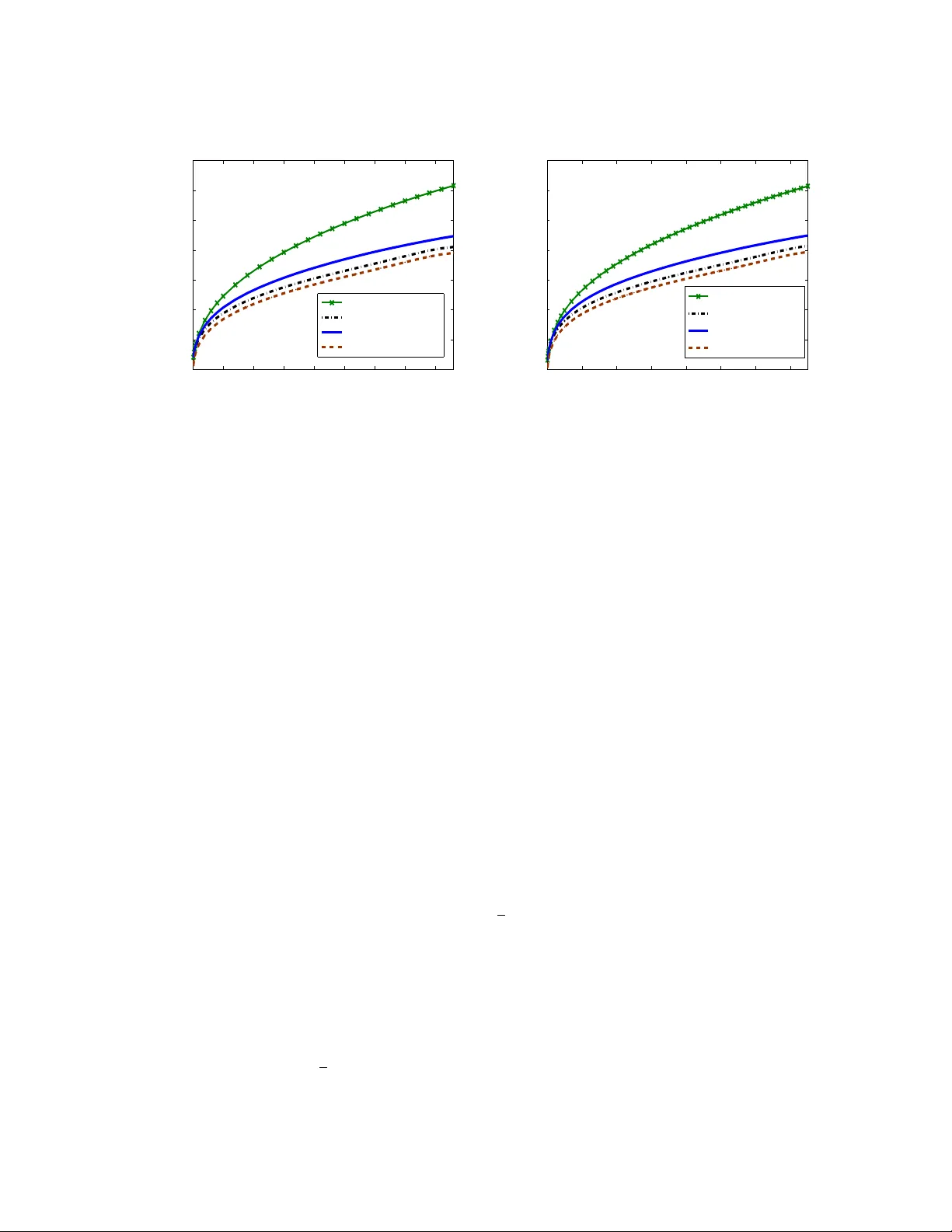
Journal of Artiﬁcial Intelligence Researc h 35 (2009) 193-234 Submitted 4/08; published 6/09 T ransductiv e Rademac her Complexit y and its Applications Ran El-Y aniv rani@cs.technion.ac.il Dmitry P ec hy on y pechyony@cs.technion.ac.il Dep artment of Computer Scienc e T e chnion - Isr ael Institute of T e chnolo gy Haifa, 32000, Isr ael Abstract W e dev elop a technique for deriving data-dependent error bounds for transductiv e learning algorithms based on transductive Rademac her complexity . Our technique is based on a no vel general error b ound for transduction in terms of transductive Rademac her com- plexit y , together with a nov el b ounding technique for Rademacher av erages for particular algorithms, in terms of their “unlab eled-lab eled” representation. This technique is relev ant to many adv anced graph-based transductive algorithms and we demonstrate its eﬀectiv e- ness by deriving error b ounds to three well kno wn algorithms. Finally , we present a new P AC-Ba yesian b ound for mixtures of transductive algorithms based on our Rademacher b ounds. 1. Introduction Alternativ e learning mo dels that utilize unlab eled data hav e received considerable attention in the past few years. Tw o prominen t mo dels are semi-supervised and transductiv e learn- ing. The main attraction of these mo dels is theoretical and empirical evidence (Chap elle, Sc h¨ olk opf, & Zien, 2006) indicating that they can often allow for more eﬃcient and signiﬁ- can tly faster learning in terms of sample complexit y . In this pap er we supp ort the theoretical evidence by pro viding risk b ounds for a n umber of state-of-the-art transductive algorithms. These b ounds utilize both lab eled and unlab eled examples and can be muc h tigh ter than the b ounds relying on lab eled examples alone. Here w e fo cus on distribution-free transductive learning. In this setting we are given a lab eled training sample as w ell as an unlabeled test sample. The goal is to guess the lab els of the given test points as accurately as possible 1 . Rather than generating a general hypothesis capable of predicting the label of any p oint, as in inductiv e learning, it is adv o cated b y V apnik (1982) that we should aim in transduction to solve an easier problem b y transferring kno wledge directly from the lab eled p oin ts to the unlab eled ones. T ransductive learning w as already prop osed and brieﬂy studied more than thirty years ago b y V apnik and Chervonenkis (1974), but only lately has it b een empirically recognized that transduction can often facilitate more eﬃcient or accurate learning than the tradi- tional sup ervised learning approac h (Chap elle et al., 2006). This recognition has motiv ated a ﬂurry of recent activit y focusing on transductiv e learning, with man y new algorithms 1. Man y pap ers refer to this mo del as semi-sup ervised learning. Ho wev er, the setting of semi-sup ervised learning is diﬀerent from transduction. In semi-supervised learning the learner is given randomly drawn training set consisting of lab eled and unlab eled examples. The goal of the learner is to generate a h yp othesis providing accurate predictions on the unse en examples. c ° 2009 AI Access F oundation. All rights reserv ed. El-Y aniv & Pechyony and heuristics b eing proposed. Nev ertheless, issues such as the iden tiﬁcation of “univer- sally” eﬀective learning principles for transduction remain unresolv ed. Statistical learning theory provides a principled approac h for attacking such questions through the study of error b ounds. F or example, in inductive learning such bounds hav e pro ven instrumen tal in c haracterizing learning principles and deriving practical algorithms (V apnik, 2000). In this paper w e consider the classiﬁcation setting of transductiv e learning. So far, sev eral general error b ounds for transductive classiﬁcation ha v e been dev elop ed b y V ap- nik (1982), Blum and Langford (2003), Derb eko, El-Y aniv, and Meir (2004), El-Y aniv and P ech y ony (2006). W e contin ue this fruitful line of research and develop a new technique for deriving explicit data-dependent error bounds. These b ounds are less tigh t than im- plicit ones, developed by V apnik and b y Blum and Langford. Ho wev er the explicit b ounds ma y p oten tially b e used for mo del selection and guide the dev elopmen t of new learning algorithms. Our technique consists of tw o parts. In the ﬁrst part we dev elop a nov el general error b ound for transduction in terms of transductive Rademacher complexit y . While this b ound is syntactically similar to kno wn inductive Rademac her b ounds (see, e.g., Bartlett & Mendel- son, 2002), it is fundamentally diﬀeren t in the sense that the transductiv e Rademacher com- plexit y is computed with resp ect to the hypothesis space that can b e c hosen after observing unlab eled training and test examples. This opp ortunit y is unav ailable in the inductive setting where the hypothesis space must b e ﬁxed b efor e any example is observed. The second part of our b ounding technique is a generic metho d for b ounding Rademacher complexit y of transductive algorithms based on their unlab ele d-lab ele d r epr esentation (ULR) . In this representation the soft-classiﬁcation v ector generated by the algorithm is a pro duct U α , where U is a matrix that dep ends on the unlab eled data and α is a vector that ma y dep end on all given information, including the lab eled training set. An y transductive al- gorithm has inﬁnite num b er of ULRs, including a trivial ULR, with U b eing an identit y matrix. W e show that many state-of-the-art algorithms hav e non-trivial ULR leading to non-trivial error b ounds. Based on ULR representation w e b ound Rademacher complexit y of transductiv e algorithms in terms of the sp ectrum of the matrix U in their ULR. This b ound justiﬁes the sp ectral transformations, developed b y Chap elle, W eston, and Sc h¨ olk opf (2003), Joac hims (2003), Johnson and Zhang (2008), that are commonly done to impro ve the p erformance of transductiv e algorithms. W e instantiate the Rademac her complexit y b ound for the “consistency metho d” of Zhou et al. (2004), the sp ectral graph transducer (SGT) algorithm of Joac hims (2003) and the Tikhonov regularization algorithm of Belkin, Matv eev a, and Niy ogi (2004). The bounds obtained for these algorithms are explicit and can b e easily computed. W e also sho w a simple Monte-Carlo scheme for b ounding the Rademacher complexit y of an y transductive algorithm using its ULR. W e demonstrate the eﬃcacy of this scheme for the “consistency metho d” of Zhou et al. (2004). Our ﬁnal contribution is a P AC-Ba y esian b ound for transductiv e mixture algorithms. This result, whic h is stated in Theorem 4, is obtained as a consequence of Theorem 2 using the techniques of Meir and Zhang (2003). This result motiv ates the use of ensem ble metho ds in transduction that are y et to b e explored in this setting. The pap er has the follo wing structure. In Section 1.1 we survey the results that are closely related to our w ork. In Section 2 w e deﬁne our learning mo del and transductive 2 Transductive Rademacher Complexity and its Applica tions Rademac her complexity . In Section 3 w e dev elop a nov el concentration inequality for func- tions o v er partitions of the ﬁnite set of points. This inequalit y and transductive Rademac her complexit y are used in Section 4 to derive uniform risk b ound, which dep ends on trans- ductiv e Rademac her complexit y . In Section 5 we introduce a generic metho d for b ounding Rademac her complexity of any transductive algorithm using its unlab eled-lab eled represen- tation. In Section 6 w e exemplify this technique to obtain explicit risk b ounds for sev eral kno wn transductive algorithms. Finally , in Section 7 w e instan tiate our risk bound to transductiv e mixture algorithms. W e discuss directions for future research in Section 8. The technical pro ofs of our results are presented in App endices A-I. Preliminary (and shorter) version of this pap er has app eared in the Pro ceedings of the 20th Annual Conference on Learning Theory , page 157–171, 2007. 1.1 Related W ork V apnik (1982) presented the ﬁrst general 0/1 loss b ounds for transductiv e classiﬁcation. His b ounds are implicit in the sense that tail probabilities are speciﬁed in the bound as the outcome of a computational routine. V apnik’s b ounds can b e reﬁned to include prior “b eliefs” as noted by Derb ek o et al. (2004). Similar implicit but somewhat tigh ter b ounds w ere developed b y Blum and Langford (2003) for the 0/1 loss case. Explicit P AC-Ba yesian transductiv e b ounds for any b ounded loss function were presented by Derb eko et al. (2004). Catoni (2004, 2007) and Audibert (2004) dev elop ed P A C-Bay esian and VC dimension- based risk b ounds for the special case when the size of the test set is a m ultiple of the size of the training set. Unlik e our P AC-Ba y esian b ound, the published transductive P AC- Ba yesian b ounds hold for deterministic hypotheses and for Gibbs classiﬁers. The b ounds of Balcan and Blum (2006) for semi-sup ervised learning also hold in the transductive setting, making them conceptually similar to some transductive P A C-Bay esian bounds. General error b ounds based on stabilit y w ere dev elop ed by El-Y aniv and Pec h yon y (2006). Eﬀectiv e applications of the general bounds mentioned ab ov e to particular algorithms or “learning principles” is not automatic. In the case of the P A C-Bay esian b ounds several suc h successful applications w ere presented in terms of appropriate “priors” that promote v arious structural prop erties of the data (see, e.g., Derb eko et al., 2004; El-Y aniv & Gerzon, 2005; Hanneke, 2006). Ad-ho c b ounds for particular algorithms were developed b y Belkin et al. (2004) and b y Johnson and Zhang (2007). Unlik e other b ounds (including ours) the b ound of Johnson and Zhang do es not dep end on the empirical error but only on the prop erties of the hypothesis space. If the size of the training and test set increases then their b ound con v erges to zero 2 . Thus the b ound of Johnson and Zhang eﬀectiv ely prov es the consistency of transductive algorithms that they consider. How ever this b ound holds only if the hyperparameters of those algorithms are chosen w.r.t. to the unknown test lab els. Hence the b ound of Johnson and Zhang cannot b e computed explicitly . Error b ounds based on Rademac her complexity were in tro duced b y Koltchinskii (2001) and are a w ell-established topic in induction (see Bartlett & Mendelson, 2002, and references therein). The ﬁrst Rademac her transductiv e risk bound w as presen ted by Lanc kriet et al. (2004, Theorem 24). This bound, whic h is a straigh tforward extension of the inductiv e 2. in all other known explicit b ounds the increase of training and test sets decreases only the slack term but not the empirical error. 3 El-Y aniv & Pechyony Rademac her techniques of Bartlett and Mendelson (2002), is limited to the special case when training and test sets are of equal size. The b ound presen ted here o vercomes this limitation. 2. Deﬁnitions In Section 2.1 w e provide a formal deﬁnition of our learning mo del. Then in Section 2.2 we deﬁne transductiv e Rademacher complexity and compare it with its inductive coun terpart. 2.1 Learning Mo del In this pap er we use a distribution-free transductive mo del, as deﬁned by V apnik (1982, Section 10.1, Setting 1). Consider a ﬁxed set S m + u M = { ( x i , y i ) } m + u i =1 of m + u points x i in some space together with their lab els y i . The learner is provided with the (unlab eled) ful l-sample X m + u M = { x i } m + u i =1 . A set consisting of m p oints is selected from X m + u uniformly at random among all subsets of size m . These m p oints together with their lab els are giv en to the learner as a tr aining set . Re-num bering the p oints w e denote the unlab eled training set points by X m M = { x 1 , . . . , x m } and the lab eled training set b y S m M = { ( x i , y i ) } m i =1 . The set of unlab eled points X u M = { x m +1 , . . . , x m + u } = X m + u \ X m is called the test set . The learner’s goal is to predict the lab els of the test p oin ts in X u based on S m ∪ X u . Remark 1 In our le arner mo del e ach example x i has unique lab el y i . However we al low that for i 6 = j , x i = x j but y i 6 = y j . The choice of the set of m p oints as describ ed ab o ve can b e view ed in three equiv alent w ays: 1. Drawing m p oin ts from X m + u uniformly without r eplac ement . Due to this draw, the p oin ts in the training and test sets are dep endent . 2. Random p ermutation of the full sample X m + u and c ho osing the ﬁrst m p oints as a training set. 3. Random partitioning of m + u p oin ts in to tw o disjoint sets of m and u p oints. T o emphasize diﬀerent asp ects of the transductiv e learning mo del, throughout the pap er w e use interc hangeably these three views on the generation of the training and test sets. This pap er fo cuses on binary learning problems where lab els y ∈ {± 1 } . The learning algorithms we consider generate “soft classiﬁcation” v ectors h = ( h (1) , . . . h ( m + u )) ∈ R m + u , where h ( i ) (or h ( x i )) is the soft, or conﬁdence-rated, lab el of example x i giv en by the “h yp othesis” h . F or actual (binary) classiﬁcation of x i the algorithm outputs sgn( h ( i )). W e denote by H out ⊆ R m + u the set of all p ossible soft classiﬁcation v ectors (ov er all p ossible tranining/test partitions) that are generated by the algorithm. Based on the full-sample X m + u , the algorithm selects an h yp othesis space H ⊆ R m + u of soft classiﬁcation hypotheses. Note that H out ⊆ H . Then, given the lab els of training p oin ts the algorithm outputs one hypothesis h from H out ∩ H for classiﬁcation. The goal of the transductive learner is to ﬁnd a hypothesis h minimizing the test err or L u ( h ) M = 4 Transductive Rademacher Complexity and its Applica tions 1 u P m + u i = m +1 ` ( h ( i ) , y i ) w.r.t. the 0 / 1 loss function ` . The empiric al err or of h is b L m ( h ) M = 1 m P m i =1 ` ( h ( i ) , y i ) and the ful l sample err or of h is L m + u ( h ) M = 1 m + u P m + u i =1 ` ( h ( i ) , y i ). In this work w e also use the margin loss function ` γ . F or a p ositiv e real γ , ` γ ( y 1 , y 2 ) = 0 if y 1 y 2 ≥ γ and ` γ ( y 1 , y 2 ) = min { 1 , 1 − y 1 y 2 /γ } otherwise. The empiric al (mar gin) err or of h is b L γ m ( h ) M = 1 m P m i =1 ` γ ( h ( i ) , y i ). W e denote by L γ u ( h ) the margin error of the test set and b y L γ m + u ( h ) the margin full sample error. W e denote by I s r , r < s , the set of natural n um b ers { r, r + 1 , . . . , s } . Throughout the pap er w e assume that the vectors are column ones. W e mark all vectors with the b oldface. 2.2 T ransductive Rademac her Complexit y W e adapt the inductive Rademacher complexit y to our transductive setting but generalize it a bit to also include “neutral” Rademacher v alues. Deﬁnition 1 (T ransductiv e Rademac her complexity) L et V ⊆ R m + u and p ∈ [0 , 1 / 2] . L et σ = ( σ 1 , . . . , σ m + u ) T b e a ve ctor of i.i.d. r andom variables such that σ i M =      1 with probability p ; − 1 with probability p ; 0 with probability 1 − 2 p. (1) The transductiv e Rademacher complexit y with p ar ameter p is R m + u ( V , p ) M = µ 1 m + 1 u ¶ · E σ ½ sup v ∈V σ T · v ¾ . The need for this no v el deﬁnition of Rademac her complexity is technical. Tw o main issues that lead to the new deﬁnition are: 1. The need to b ound the test error L u ( h ) = 1 u P m + u i = m +1 ` ( h ( i ) , y i ). Notice that in induc- tiv e risk b ounds the standard deﬁnition of Rademacher complexit y (see Deﬁnition 2 b elo w), with binary v alues of σ i , is used to b ound the generalization error, which is an inductive analogue of the full sample error L m + u ( h ) = 1 m + u P m + u i =1 ` ( h ( i ) , y i ). 2. Diﬀerent sizes ( m and u resp ectively) of training and test set. See Section 4.1 for more tec hnical details that lead to the ab ov e deﬁnition of Rademac her complexit y . F or the sak e of comparison we also state the inductiv e deﬁnition of Rademac her com- plexit y . Deﬁnition 2 (Inductiv e Rademac her complexity , Koltchinskii, 2001) L et D b e a pr ob ability distribution over X . Supp ose that the examples X n = { x i } n i =1 ar e sample d in- dep endently fr om X ac c or ding to D . L et F b e a class of functions mapping X to R . L et σ = { σ i } n i =1 b e an indep endent uniform {± 1 } -value d r andom variables, σ i = 1 with pr ob- ability 1 / 2 and σ i = − 1 with the same pr ob ability. The empirical Rademac her complex- 5 El-Y aniv & Pechyony it y is 3 b R (ind) n ( F ) M = 2 n E σ © sup f ∈F P n i =1 σ i f ( x i ) ª and the Rademac her complexity of F is R (ind) n ( F ) M = E X n ∼D n n b R (ind) n ( F ) o . F or the case p = 1 / 2, m = u and n M = m + u w e ha v e that R m + u ( V ) = 2 b R (ind) m + u ( V ). Whenev er p < 1 / 2, some Rademac her v ariables will attain (neutral) zero v alues and reduce the complexity (see Lemma 1). W e use this prop erty to tighten our b ounds. Notice that the transductive complexity is an empirical quantit y that do es not dep end on any underlying distribution, including the one o ver the choices of the training set. Since in distribution-free transductive mo del the unlab eled full sample of training and test p oints is ﬁxed, in transductive Rademac her complexit y we don’t need the outer exp ectation, which app ears in the inductive deﬁnition. Also, the transductive complexity dep ends on b oth the (unlab eled) training and test p oints whereas the inductive complexity only dep ends only on the (unlab eled) training p oin ts. The following lemma, whose pro of app ears in App endix A, states that R m + u ( V , p ) is monotone increasing with p . The proof is based on the tec hnique used in the pro of of Lemma 5 in the pap er of Meir and Zhang (2003). Lemma 1 F or any V ⊆ R m + u and 0 ≤ p 1 < p 2 ≤ 1 / 2 , R m + u ( V , p 1 ) < R m + u ( V , p 2 ) . In the forthcoming results w e utilize the transductive Rademac her complexity with p 0 M = mu ( m + u ) 2 . W e abbreviate R m + u ( V ) M = R m + u ( V , p 0 ). By Lemma 1, all our b ounds also apply to R m + u ( V , p ) for all p > p 0 . Since p 0 < 1 2 , the Rademac her complexity inv olved in our results is strictly smaller than the standard inductiv e Rademacher complexity deﬁned o ver X m + u . Also, if transduction approaches the induction, namely m is ﬁxed and u → ∞ , then b R (ind) m + u ( V ) → 2 R m + u ( V ). 3. Concentration Inequalities for F unctions o ver P artitions In this section we dev elop a nov el concen tration inequality for functions o ver partitions and compare it to the several kno wn ones. Our concentration inequality is utilized in the deriv ation of the forthcoming risk b ound. Let Z M = Z m + u 1 M = ( Z 1 , . . . , Z m + u ) b e a r andom p ermutation ve ctor where the v ariable Z k , k ∈ I m + u 1 , is the k th comp onent of a p erm utation of I m + u 1 that is chosen uniformly at random. Let Z ij b e a perturb ed p ermutation vector obtained b y exc hanging the v alues of Z i and Z j in Z . An y function f on p ermutations of I m + u 1 is called ( m, u ) -p ermutation symmet- ric if f ( Z ) M = f ( Z 1 , . . . , Z m + u ) is symmetric on Z 1 , . . . , Z m as well as on Z m +1 , . . . , Z m + u . In this section we present a no vel concentration inequalit y for ( m, u )-p ermutation sym- metric functions. Note that an ( m, u )-permutation symmetric function is essen tially a func- tion o ver the partition of m + u items into sets of sizes m and u . Thus, the forthcoming inequalities of Lemmas 2 and 3, while b eing stated for ( m, u )-p ermutation symmetric func- tions, also hold in exactly the same form for functions ov er partitions. Conceptually it is 3. The original deﬁnition of Rademacher complexit y , as given b y Koltchinskii (2001), is slightly diﬀerent from the one presen ted here, and contains sup f ∈F ˛ ˛ P n i =1 σ i f ( x i ) ˛ ˛ instead of sup f ∈F P n i =1 σ i f ( x i ). How- ev er, from the conceptual p oint of view, Deﬁnition 2 and the one giv en by Koltchinskii are equiv alen t. 6 Transductive Rademacher Complexity and its Applica tions more conv enient to view our results as concen tration inequalities for functions ov er par- titions. How ev er, from a tec hnical p oint of view w e ﬁnd it more conv enient to consider ( m, u )-p erm utation symmetric functions. The follo wing lemma (that will b e utilized in the pro of of Theorem 1) presen ts a con- cen tration inequality that is an extension of Lemma 2 of El-Y aniv and P ech y ony (2006). The pro of (app earing in App endix B) relies on McDiarmid’s inequalit y (McDiarmid, 1989, Corollary 6.10) for martingales. Lemma 2 L et Z b e a r andom p ermutation ve ctor over I m + u 1 . L et f ( Z ) b e an ( m, u ) - p ermutation symmetric function satisfying ¯ ¯ f ( Z ) − f ( Z ij ) ¯ ¯ ≤ β for al l i ∈ I m 1 , j ∈ I m + u m +1 . Then P Z { f ( Z ) − E Z { f ( Z ) } ≥ ² } ≤ exp µ − 2 ² 2 ( m + u − 1 / 2) muβ 2 µ 1 − 1 2 max( m, u ) ¶¶ . (2) The right hand side of (2) is appro ximately exp ³ − 2 ² 2 β 2 ¡ 1 m + 1 u ¢ ´ . A similar, but less tight inequalit y can b e obtained by reduction of the draw of random p ermutation to the draw of min( m, u ) indep endent random v ariables and application of the b ounded diﬀerence in- equalit y of McDiarmid (1989): Lemma 3 Supp ose that the c onditions of L emma 2 hold. Then P Z { f ( Z ) − E Z { f ( Z ) } ≥ ² } ≤ exp µ − 2 ² 2 β 2 min( m, u ) ¶ . (3) The pro of of Lemma 3 app ears in App endix C. Remark 2 The ine qualities develop e d in Se ction 5 of T alagr and (1995) imply a c onc entr a- tion ine quality that is similar to (3), but with worse c onstants. The inequality (2) is deﬁned for an y ( m, u )-p ermutation symmetric function f . By sp ecializing f w e obtain the follo wing t wo concen tration inequalities: Remark 3 If g : I m + u 1 → { 0 , 1 } and f ( Z ) = 1 u P m + u i = m +1 g ( Z i ) − 1 m P m i =1 g ( Z i ) , then E Z { f ( Z ) } = 0 . Mor e over, for any i ∈ I m 1 , j ∈ I m + u m +1 , | f ( Z ) − f ( Z ij ) | ≤ 1 m + 1 u . Ther efor e, by sp e cializing (2) for such f we obtain P Z ( 1 u m + u X i = m +1 g ( Z i ) − 1 m m X i =1 g ( Z i ) ≥ ² ) ≤ exp µ − ² 2 mu ( m + u − 1 / 2) ( m + u ) 2 · 2 max( m, u ) − 1 max( m, u ) ¶ . (4) The right hand side of (4) is appr oximately exp ³ − 2 ² 2 mu m + u ´ . The ine quality (4) is an ex- plicit (and lo oser) version of V apnik’s absolute b ound (se e El-Y aniv & Gerzon, 2005). We note that using (2) we wer e unable to obtain an explicit version of V apnik’s r elative b ound (ine quality 10.14 of V apnik, 1982). 7 El-Y aniv & Pechyony Remark 4 If g : I m + u 1 → { 0 , 1 } , f ( Z ) = 1 m P m i =1 g ( Z i ) , then E Z { f ( Z ) } = 1 m + u P m + u i =1 g ( Z i ) . Mor e over, for any i ∈ I m 1 , j ∈ I m + u m +1 , | f ( Z ) − f ( Z ij ) | ≤ 1 m . Ther efor e, by sp e cializing (2) for such f we obtain P Z ( 1 m m X i =1 g ( Z i ) − 1 m + u m + u X i =1 g ( Z i ) ≥ ² ) ≤ exp µ − ² 2 ( m + u − 1 / 2) m u · 2 max( m, u ) − 1 max( m, u ) ¶ . (5) The right hand side of (5) is appr oximately exp ³ − 2 ² 2 ( m + u ) m u ´ . This b ound is asymptotic al ly the same as fol lowing b ound, which was develop e d by Serﬂing (1974): P Z ( 1 m m X i =1 g ( Z i ) − 1 m + u m + u X i =1 g ( Z i ) ≥ ² ) ≤ exp µ − 2 ² 2 ( m + u ) m u + 1 ¶ . 4. Uniform Rademacher Error Bound In this section we dev elop a transductive risk b ound, whic h is based on transductiv e Rademac her complexity (Deﬁnition 1). The deriv ation follows the standard t w o-step scheme, as in induction 4 : 1. Deriv ation of a uniform concentration inequality for a set of vectors (or functions). This inequality dep ends on the Rademacher complexit y of the set. After substituting to the vectors (or functions) the v alues of the loss functions, we obtain an error b ound dep ending on the Rademacher complexity of the v alues of the loss function. This step is done in Section 4.1. 2. In order to b ound the Rademac her complexit y in terms of the properties of the hy- p othesis space, the Rademacher complexity is ‘translated’, using its contraction prop- ert y (Ledoux & T alagrand, 1991, Theorem 4.12), from the domain of loss function v alues to the domain of soft hypotheses from the hypothesis space. This step is done in Section 4.2. As we sho w in Sections 4.1 and 4.2, the adaptation of b oth these steps to the transductive setting is not immediate and inv olves several no vel ideas. In Section 4.3 w e combine the results of these tw o steps and obtain a transductiv e Rademac her risk bound. W e also pro vide a thorough comparison of our risk b ound with the corresp onding inductive b ound. 4.1 Uniform Concentration Inequalit y for a Set of V ectors As in induction (Koltchinskii & Panc henk o, 2002), our deriv ation of a uniform concentration inequalit y for a set of v ectors consists of three steps: 1. Introduction of the “ghost sample”. 2. Bounding the suprem um sup h ∈H g ( h ), where g ( h ) is some random real-v alued func- tion, with its exp ectation using a concen tration inequalit y for functions of random v ariables. 4. This sc heme was in tro duced by Koltchinskii and Panc henk o (2002). The examples of other uses of this tec hnique can b e found in the pap ers of Bartlett and Mendelson (2002) and Meir and Zhang (2003). 8 Transductive Rademacher Complexity and its Applica tions 3. Bounding the exp ectation of the suprem um using Rademacher v ariables. While we follo w these three steps as in induction, the establishmen t of eac h of these steps can not b e ac hieved using inductive techniques. Throughout this section, after p erforming the deriv ation of each step in transductive context w e discuss its diﬀerences from its inductive coun terpart. W e introduce sev eral new deﬁnitions. Let V b e a set of vectors in [ B 1 , B 2 ] m + u , B 1 ≤ 0, B 2 ≥ 0 and set B M = B 2 − B 1 , B max = max( | B 1 | , | B 2 | ). Consider tw o indep endent p erm utations of I m + u 1 , Z and Z 0 . F or any v ∈ V denote by v ( Z ) M = ( v ( Z 1 ) , v ( Z 2 ) , . . . , v ( Z m + u )) , the vector v p erm uted according to Z . W e use the follo wing abbreviations for a verages of v ov er subsets of its comp onents: H k { v ( Z ) } M = 1 m P k i =1 v ( Z i ), T k { v ( Z ) } M = 1 u P m + u i = k +1 v ( Z i ) (note that H stands for ‘head’ and T , for ’tail’). In the sp ecial case where k = m we set H { v ( Z ) } M = H m { v ( Z ) } , and T { v ( Z ) } M = T m { v ( Z ) } . The uniform concentration inequalit y that we develop shortly states that for any δ > 0, with probabilit y at least 1 − δ o ver random p erm utation Z of I m + u 1 , for an y v ∈ V , T { v ( Z ) } ≤ H { v ( Z ) } + R m + u ( V ) + O Ã s 1 min( m, u ) ln 1 δ ! . Step 1: Intr o duction of the ghost sample. W e denote b y ¯ v M = 1 m + u P m + u i =1 v ( i ) the a verage comp onent of v . F or an y v ∈ V and an y p erm utation Z of I m + u 1 w e ha ve T { v ( Z ) } = H { v ( Z ) } + T { v ( Z ) } − H { v ( Z ) } ≤ H { v ( Z ) } + sup v ∈V h T { v ( Z ) } − ¯ v + ¯ v − H { v ( Z ) } i = H { v ( Z ) } + sup v ∈V h T { v ( Z ) } − E Z 0 T { v ( Z 0 ) } + E Z 0 H { v ( Z 0 ) } − H { v ( Z ) } i ≤ H { v ( Z ) } + E Z 0 sup v ∈V h T { v ( Z ) } − T { v ( Z 0 ) } + H { v ( Z 0 ) } − H { v ( Z ) } i | {z } M = ψ ( Z ) . (6) Remark 5 In this derivation the “ghost sample” is a p ermutation Z 0 of m + u elements dr awn fr om the same distribution as Z . In inductive R ademacher-b ase d risk b ounds the ghost sample is a new tr aining set of size m , indep endently dr awn fr om the original one. Note that in our tr ansductive setting the ghost sample c orr esp onds to the indep endent dr aw of tr aining/test set p artition, which is e quivalent to the indep endent dr aw of r andom p er- mutation Z 0 . Remark 6 In principle we c ould avoid the intr o duction of the ghost sample Z 0 and c onsider m elements in H { v ( Z ) } as ghosts of u elements in T { v ( Z ) } . This appr o ach would le ad to 9 El-Y aniv & Pechyony a new deﬁnition of R ademacher aver ages (with σ i = − 1 /m with pr ob ability m/ ( m + u ) and 1 /u with pr ob ability u/ ( m + u ) ). With this deﬁnition we c an obtain Cor ol lary 1. However, sinc e the distribution of alternative R ademacher aver ages is not symmetric ar ound zer o, te chnic al ly we do not know how to pr ove the L emma 5 (the c ontr action pr op erty). Step 2: Bounding the supr emum with its exp e ctation. Let S M = m + u ( m + u − 1 / 2)(1 − 1 / (2 max( m,u ))) . F or suﬃcien tly large m and u , the v alue of S is al- most 1. The function ψ ( Z ) is ( m, u )-permutation symmetric in Z . It can be v eriﬁed that | ψ ( Z ) − ψ ( Z ij ) | ≤ B ¡ 1 m + 1 u ¢ . Therefore, w e can apply Lemma 2 with β M = B ¡ 1 m + 1 u ¢ to ψ ( Z ). W e obtain, with probability of at least 1 − δ o v er random p ermutation Z of I m + u 1 , for all v ∈ V : T { v ( Z ) } ≤ H { v ( Z ) } + E Z { ψ ( Z ) } + B s S 2 µ 1 m + 1 u ¶ ln 1 δ . (7) Remark 7 In induction this step is p erforme d using an applic ation of McDiarmid’s b ounde d diﬀer enc e ine quality (McDiarmid, 1989, L emma 1.2). We c annot apply this ine quality in our setting sinc e the function under the supr emum (i.e. ψ ( Z ) ) is not a function over in- dep endent variables, but r ather over p ermutations. Our L emma 2 r eplac es the b ounde d diﬀer enc e ine quality in this step. Step 3: Bounding the exp e ctation over the supr emum using R ademacher r andom variables. Our goal is to b ound the exp ectation E Z { ψ ( Z ) } . This is done in the following lemma. Lemma 4 L et Z b e a r andom p ermutation of I m + u 1 . L et c 0 M = q 32 ln(4 e ) 3 < 5 . 05 . Then E Z { ψ ( Z ) } ≤ R m + u ( V ) + c 0 B max µ 1 u + 1 m ¶ p min( m, u ) . Pro of: The proof is based on ideas from the pro of of Lemma 3 from Bartlett and Mendelson (2002). F or technical conv enience w e use the following deﬁnition of pairwise Rademacher v ariables. Deﬁnition 3 (P airwise Rademac her v ariables) L et v = ( v (1) , . . . , v ( m + u )) ∈ R m + u . L et V b e a set of ve ctors fr om R m + u . L et ˜ σ = { ˜ σ i } m + u i =1 b e a ve ctor of i.i.d. r andom variables deﬁne d as: ˜ σ i = ( ˜ σ i, 1 , ˜ σ i, 2 ) =            ¡ − 1 m , − 1 u ¢ with probability mu ( m + u ) 2 ; ¡ − 1 m , 1 m ¢ with probability m 2 ( m + u ) 2 ; ¡ 1 u , 1 m ¢ with probability mu ( m + u ) 2 ; ¡ 1 u , − 1 u ¢ with probability u 2 ( m + u ) 2 . (8) W e obtain Deﬁnition 3 from Deﬁnition 1 (with p = mu ( m + u ) 2 ) in the follo wing wa y . If the Rademac her v ariable σ i = 1 then w e split it to ˜ σ i = ¡ 1 u , 1 m ¢ . If the Rademacher v ariable 10 Transductive Rademacher Complexity and its Applica tions σ i = − 1 then we split it to ˜ σ i = ¡ − 1 m , − 1 u ¢ . If the Rademacher v ariable σ i = 0 then we split it randomly to ¡ − 1 m , 1 m ¢ or ¡ 1 u , − 1 u ¢ . The ﬁrst comp onent of ˜ σ i indicates if the i th comp onen t of v is in the ﬁrst elements of v ( Z ) or in the last u elements of v ( Z ). If the former case the v alue of ˜ σ i is − 1 m and in the latter case the v alue of ˜ σ i is 1 u . The second comp onen t of ˜ σ i has the same meaning as the ﬁrst one, but with Z replaced b y Z 0 . The v alues ± 1 m and ± 1 u are exactly the co eﬃcients app earing inside T { v ( Z ) } , T { v ( Z 0 ) } , H { v ( Z 0 ) } and H { v ( Z ) } in (6). These co eﬃcien ts are random and their distribution is induced by the uniform distribution ov er p ermutations. In the course of the pro of w e will establish the precise relation betw een the distribution of ± 1 m and ± 1 u co eﬃcien ts and the distribution (8) of pairwise Rademac her v ariables. It is easy to v erify that R m + u ( V ) = E ˜ σ ( sup v ∈V m + u X i =1 ( ˜ σ i, 1 + ˜ σ i, 2 ) v ( i ) ) . (9) Let n 1 , n 2 and n 3 b e the num b er of random v ariables ˜ σ i realizing the v alue ¡ − 1 m , − 1 u ¢ , ¡ − 1 m , 1 m ¢ , ¡ 1 u , 1 m ¢ , resp ectiv ely . Set N 1 M = n 1 + n 2 and N 2 M = n 2 + n 3 . Note that the n i ’s and N i ’s are random v ariables. Denote by Rad the distribution of ˜ σ deﬁned by (8) and by Rad ( N 1 , N 2 ), the distribution Rad conditioned on the even ts n 1 + n 2 = N 1 and n 2 + n 3 = N 2 . W e deﬁne s ( N 1 , N 2 ) M = E ˜ σ ∼ Rad ( N 1 ,N 2 ) ( sup v ∈V m + u X i =1 ( ˜ σ i, 1 + ˜ σ i, 2 ) v ( i ) ) . The rest of the pro of is based on the following three claims: Claim 1. R m + u ( V ) = E N 1 ,N 2 { s ( N 1 , N 2 ) } . Claim 2. E Z { ψ ( Z ) } = s ( E ˜ σ N 1 , E ˜ σ N 2 ). Claim 3. s ( E ˜ σ N 1 , E ˜ σ N 2 ) − E N 1 ,N 2 { s ( N 1 , N 2 ) } ≤ c 0 B max ¡ 1 u + 1 m ¢ √ m . Ha ving established these three claims w e immediately obtain E Z { g ( Z ) } ≤ ˜ R m + u ( V ) + c 0 B max µ 1 u + 1 m ¶ √ m . (10) The en tire dev elopment is symmetric in m and u and, therefore, w e also obtain the same result but with √ u instead of √ m . By taking the minim um of (10) and the symmetric b ound (with √ u ) we establish the theorem. The pro of of the ab o ve three claims app ears in App endix D. ¤ Remark 8 The te chnique we use to b ound the exp e ctation of the supr emum is mor e c om- plic ate d than the te chnique of Koltchinskii and Panchenko (2002) that is c ommonly use d in induction. This is c ause d by the structur e of the function under the supr emum (i.e., g ( Z ) ). F r om a c onc eptual p oint of view, this step utilizes our novel deﬁnition of tr ansduc- tive R ademacher c omplexity. By com bining (7) and Lemma 4 w e obtain the next concentration inequality , which is the main result of this section. 11 El-Y aniv & Pechyony Theorem 1 L et B 1 ≤ 0 , B 2 ≥ 0 and V b e a (p ossibly inﬁnite) set of r e al-value d ve ctors in [ B 1 , B 2 ] m + u . L et B M = B 2 − B 1 and B max M = max( | B 1 | , | B 2 | ) . L et Q M = ¡ 1 u + 1 m ¢ , S M = m + u ( m + u − 1 / 2)(1 − 1 / 2(max( m,u ))) and c 0 M = q 32 ln(4 e ) 3 < 5 . 05 . Then with pr ob ability of at le ast 1 − δ over r andom p ermutation Z of I m + u 1 , for al l v ∈ V , T { v ( Z ) } ≤ H { v ( Z ) } + R m + u ( V ) + B max c 0 Q p min( m, u ) + B r S 2 Q ln 1 δ . (11) W e defer the analysis of the slack terms B max c 0 Q p min( m, u ) and B q S 2 Q ln 1 δ to Sec- tion 4.3. W e no w instan tiate the inequality (11) to obtain our ﬁrst risk bound. The idea is to apply Theorem 1 with an appropriate instan tiation of the set V so that T { v ( Z ) } will corresp ond to the test error and H { v ( Z ) } to the empirical error. F or a true (unknown) lab eling of the full-sample y and an y h ∈ H out w e deﬁne ` y ( h ) M = ( ` ( h (1) , y 1 ) , . . . , ` ( h ( m + u ) , y m + u )) and set L H = { v : v = ` y ( h ) , h ∈ H out } . Thus ` y ( h ) is a v ector of the v alues of the 0 / 1 loss ov er all full sample examples, when transductive algorithm is op erated on some training/test partition. The set L H is the set of all p ossible vectors ` y ( h ), o ver all p ossible training/test partitions. W e apply Theorem 1 with V M = L H , v M = ` ( h ), B max = B = 1 and obtain the follo wing corollary: Corollary 1 L et Q , S and c 0 b e as deﬁne d in The or em 1. F or any δ > 0 , with pr ob ability of at le ast 1 − δ over the choic e of the tr aining set fr om X m + u , for al l h ∈ H out , L u ( h ) ≤ b L m ( h ) + R m + u ( L H ) + B max c 0 Q p min( m, u ) + r S 2 Q ln 1 δ . (12) W e defer the analysis of the slac k terms B max c 0 Q p min( m, u ) and B q S 2 Q ln 1 δ to Section 4.3. While the b ound (12) is obtained by a straigh tforward application of the concen tration inequalit y (11), it is not conv enien t to deal with. That’s b ecause it is not clear ho w to b ound the Rademac her complexity R m + u ( L H ) of the 0 / 1 loss v alues in terms of the prop erties of transductiv e algorithm. In the next sections w e eliminate this deﬁciency by utilizing margin loss function. 4.2 Contraction of Rademac her Complexit y The following lemma is a version of the well-kno wn ‘contraction principle’ of the theory of Rademac her av erages (see Theorem 4.12 of Ledoux & T alagrand, 1991, and Ambroladze, P arrado-Hernandez, & Shaw e-T aylor, 2007). The lemma is an adaptation, which accommo- dates the transductive Rademacher v ariables, of Lemma 5 of Meir and Zhang (2003). The pro of is pro vided in App endix E. Lemma 5 L et V ⊆ R m + u b e a set of ve ctors. L et f and g b e r e al-value d functions. L et σ = { σ i } m + u i =1 b e R ademacher variables, as deﬁne d in (1). If for al l 1 ≤ i ≤ m + u and any 12 Transductive Rademacher Complexity and its Applica tions v , v 0 ∈ V , | f ( v i ) − f ( v 0 i ) | ≤ | g ( v i ) − g ( v 0 i ) | , then E σ sup v ∈V " m + u X i =1 σ i f ( v i ) # ≤ E σ sup v ∈V " m + u X i =1 σ i g ( v i ) # . Let y = ( y 1 , . . . , y m + u ) ∈ R m + u b e a true (unknown) lab eling of the full-sample. Sim- ilarly to what w as done in the deriv ation of Corollary 1, for any h ∈ H out w e deﬁne ` y γ ( h ( i )) M = ` γ ( h ( i ) , y i ) and ` y γ ( h ) M = ( ` y γ ( h (1)) , . . . , ` Y γ ( h ( m + u ))) and set L γ H = { v : v = ` y γ ( h ) , h ∈ H out } . Noting that ` y γ satisﬁes the Lipsc hitz condition | ` y γ ( h ( i )) − ` y γ ( h 0 ( i )) | ≤ 1 γ | h ( i ) − h 0 ( i ) | , w e apply Lemma 5 with V M = L γ H , f ( v i ) M = ` y γ ( h ( i )) and g ( v i ) M = h ( i ) /γ , to get E σ ( sup h ∈H out m + u X i =1 σ i ` y γ ( h ( i )) ) ≤ 1 γ E σ ( sup h ∈H out m + u X i =1 σ i h ( i ) ) . (13) It follows from (13) that R m + u ( L γ H ) ≤ 1 γ R m + u ( H out ) . (14) 4.3 Risk Bound and Comparison with Related Results Applying Theorem 1 with V M = L γ H , v M = ` γ ( h ), B max = B = 1, and using the inequalit y (14) we obtain 5 : Theorem 2 L et H out b e the set of ful l-sample soft lab elings of the algorithm, gener ate d by op er ating it on al l p ossible tr aining/test set p artitions. The choic e of H out c an de- p end on the ful l-sample X m + u . L et c 0 = q 32 ln(4 e ) 3 < 5 . 05 , Q M = ¡ 1 u + 1 m ¢ and S M = m + u ( m + u − 1 / 2)(1 − 1 / (2 max( m,u ))) . F or any ﬁxe d γ , with pr ob ability of at le ast 1 − δ over the choic e of the tr aining set fr om X m + u , for al l h ∈ H out , L u ( h ) ≤ L γ u ( h ) ≤ b L γ m ( h ) + R m + u ( H out ) γ + c 0 Q p min( m, u ) + r S Q 2 ln 1 δ . (15) F or large enough v alues of m and u the v alue of S is close to 1. Therefore the slac k term c 0 Q p min( m, u ) + q S 2 Q ln 1 δ is of order O ³ 1 / p min( m, u ) ´ . The con vergence rate of O ³ 1 / p min( m, u ) ´ can be very slow if m is very small or u ¿ m . Slow rate for small m is not surprising, but a latter case of u ¿ m is somewhat surprising. Ho wev er note that if u ¿ m then the mean µ of u elemen ts, dra wn from m + u elements, has a large v ariance. Hence, in this case an y high-conﬁdence interv al for the estimation of µ will b e large. This conﬁdence interv al is reﬂected in the slack term of (15). 5. This b ound holds for any ﬁxe d margin parameter γ . Using the technique of the pro of of Theorem 18 of Bousquet and Elisseeﬀ (2002), we can also obtain a b ound that is uniform in γ . 13 El-Y aniv & Pechyony W e no w compare the b ound (15) with the Rademacher-based inductive risk b ounds. W e use the following v ariant of Rademac her-based inductiv e risk b ound of Meir and Zhang (2003): Theorem 3 L et D b e a pr ob ability distribution over X . Supp ose that a set of examples S m = { ( x i , y i ) } m i =1 is sample d i.i.d. fr om X ac c or ding to D . L et F b e a class of functions e ach maps X to R and b R (ind) m ( F ) b e the empiric al R ademacher c omplexity of F (Deﬁni- tion 2). L et L ( f ) = E ( x,y ) ∼D { ` ( f ( x ) , y ) } and b L γ ( f ) = 1 m P m i =1 ` γ ( f ( x i ) , y i ) b e r esp e ctively the 0/1 gener alization err or and empiric al mar gin err or of f . Then for any δ > 0 and γ > 0 , with pr ob ability of at le ast 1 − δ over the r andom dr aw of S m , for any f ∈ F , L ( f ) ≤ b L γ ( f ) + b R (ind) m ( F ) γ + r 2 ln(2 /δ ) m . (16) The slac k term in the b ound (16) is of order O (1 / √ m ). The b ounds (15) and (16) are not quantitativ ely comparable. The inductiv e b ound holds with high probability o ver the random selection of m examples from some distribution D . This b ound is on av erage (generalization) error, ov er all examples in D . The transductive b ound holds with high probabilit y ov er the random selection of a training/test partition. This b ound is on the test error of some hypothesis o ver a particular set of u p oin ts. A kind of meaningful comparison can b e obtained as follo ws. Using the giv en full (transductiv e) sample X m + u , we deﬁne a corresponding inductiv e distribution D trans as the uniform distribution o v er X m + u ; that is, a training set of size m will b e generated b y sampling from X m + u m times with replacements. Giv en an inductive h yp othesis space F = { f } of function we deﬁne the transductive hypothesis space H F as a pro jection of F in to the full sample X m + u : H F = { h ∈ R m + u : ∃ f ∈ F , ∀ 1 ≤ i ≤ m + u, h ( i ) = f ( x i ) } . By such deﬁnition of H F , L ( f ) = L m + u ( h ). Our ﬁnal step tow ards a meaningful comparison would be to translate a transductiv e b ound of the form L u ( h ) ≤ b L γ m ( h ) + slack to a b ound on the av erage error of the hypothesis 6 h : L m + u ( h ) ≤ L γ m + u ( h ) = m b L γ m ( h ) + u L γ u ( h ) m + u ≤ m b L γ m ( h ) + u ³ b L γ m ( h ) + slack ´ m + u = b L γ m ( h ) + u m + u · slac k (17) W e instan tiate (17) to the b ound (15) and obtain L m + u ( h ) ≤ b L γ m ( h ) + u m + u R m + u ( H F ) γ + u m + u " c 0 Q p min( m, u ) + r S Q 2 ln 1 δ # . (18) 6. Alternativ ely , to compare (15) and (16), we could try to express the b ound (16) as the b ound on the error of f on X u (the randomly drawn subset of u examples). The b ound (16) holds for the setting of random draws with replacement. In this setting the num b er of unique training examples can b e smaller than m and thus the num ber of the remaining test examples is larger than u . Hence the dra w of m training examples with replacement do es not imply the draw of the subset of u test examples, as in transductiv e setting. Thus we cannot express the b ound (16) as the b ound on the randomly drawn X u 14 Transductive Rademacher Complexity and its Applica tions No w given a transductiv e problem we consider the corresponding inductiv e b ound obtained from (16) under the distribution D trans and compare it to the b ound (18). Note that in the inductiv e bound (16) the sampling of the training set is done with replacemen t, while in the transductiv e b ound (18) it is done without replacement. Thus, in the inductiv e case the actual num b er of distinct training examples may b e smaller than m . The b ounds (16) and (18) consist of three terms: empirical error term (ﬁrst summand in (16) and (18)), the term dep ending on the Rademacher complexity (second summand in (16) and (18)) and the slack term (third summand in (16) and third and fourth summands in (18)). The empirical error terms are the same in b oth b ounds. It is hard to compare analytically the Rademac her complexity terms. This is b ecause the inductive b ound is deriv ed for the setting of sampling with replacemen t and the transductive b ound is deriv ed for the setting of sampling without replacement. Th us, in the transductive Rademacher complexit y eac h example x i ∈ X m + u app ears in R m + u ( H out ) only once and is m ultiplied b y σ i . In con trast, due to the sampling with replacemen t, in the inductiv e Rademac her term the example x i ∈ X m + u can appear several times in b R (ind) m + u ( F ), multiplied by diﬀerent v alues of the Rademac her v ariables. Nev ertheless, in transduction we hav e a full con trol ov er the Rademacher complexit y (since we can choose H out after observing the full sample X m + u ) and can c ho ose an h yp oth- esis space H out with arbitrarily small Rademacher complexit y . In induction we choose F b efore observing an y data. Hence, if w e are lucky with the full sample X m + u then b R (ind) m + u ( F ) is small, and if we are unluc ky with X m + u then b R (ind) m + u ( F ) can b e large. Thus, under these pro visions w e can argue that the transductive Rademacher term is not larger than the inductiv e coun terpart. Finally , w e compare the slack terms in (16) and (18). If m ≈ u or m ¿ u then the slack term of (18) is of order O (1 / √ m ), which is the same as the corresp onding term in (16). But if m À u then the slac k term of (18) is of order O (1 / ( m √ u )), which is muc h smaller than O (1 / √ m ) of the slack term in (16). Based on the comparison of the corresp onding terms in (16) and (18) our conclusion is that in the regime of u ¿ m the transductiv e bound is signiﬁcan tly tigh ter than the inductiv e one. 7 5. Unlab eled-Lab eled Represen tation (ULR) of T ransductiv e Algorithms Let r b e any natural num b er and let U be an ( m + u ) × r matrix dep ending only on X m + u . Let α be an r × 1 v ector that ma y dep end on b oth S m and X u . The soft classiﬁcation output h of any transductiv e algorithm can b e represented b y h = U · α . (19) W e refer to (19) as an unlab ele d-lab ele d r epr esentation (ULR) . In this section we dev elop b ounds on the Rademac her complexit y of algorithms based on their ULRs. W e note that an y transductive algorithm has a trivial ULR, for example, b y taking r = m + u , setting U 7. The regime of u ¿ m o ccurs in the following class of applications. Giv en a large library of tagged ob jects, the goal of the learner is to assign the tags to a small quan tity of the newly arrived ob jects. The example of such application is the organization of daily news. 15 El-Y aniv & Pechyony to b e the iden tity matrix and assigning α to any desired (soft) lab els. W e are interested in “non-trivial” ULRs and provide useful b ounds for such represen tations. 8 In a “v anilla” ULR, U is an ( m + u ) × ( m + u ) matrix and α = ( α 1 , . . . , α m + u ) simply sp eciﬁes the giv en lab els in S m (where α i = y i for lab eled p oints, and α i = 0 otherwise). F rom our point of view an y v anilla ULR is not trivial b ecause α do es not encode the ﬁnal classiﬁcation of the algorithm. F or example, the algorithm of Zhou et al. (2004) straigh tforwardly admits a v anilla ULR. On the other hand, the natural (non-trivial) ULR of the algorithms of Zh u et al. (2003) and Belkin and Niy ogi (2004) are not of the v anilla t yp e. F or some algorithms it is not necessarily ob vious how to ﬁnd non-trivial ULRs. In Sections 6 we consider tw o suc h cases – in particular, the algorithms of Joachims (2003) and Belkin et al. (2004). The rest of this section is organized as follows. In Section 5.1 we presen t a generic b ound on the Rademacher complexit y of an y transductive algorithm based on its ULR. In Section 5.2 we consider a case when the matrix U is a k ernel matrix. F or this case we dev elop another b ound on the transductive Rademacher complexity . Finally , in Section 5.3 w e presen t a method of computing high-conﬁdence estimate of the transductiv e Rademac her complexit y . 5.1 Generic Bound on T ransductive Rademac her Complexit y W e no w present a b ound on the transductiv e Rademacher complexity of an y transductiv e algorithm based on its ULR. Let { λ i } r i =1 b e the singular v alues of U . W e use the w ell-known fact that k U k F ro = q P r i =1 λ 2 i , where k U k F ro M = q P i,j ( U ( i, j )) 2 is the F rob enius norm of U . Supp ose that k α k 2 ≤ µ 1 for some µ 1 . Let H out M = H out ( U ) b e the set of all p ossible outputs of the algorithm when op erated on all p ossible training/test set partitions of the full-sample X m + u . Let Q M = 1 m + 1 u . Using the abbreviation U ( i, · ) for the i th row of U and follo wing the pro of idea of Lemma 22 of Bartlett and Mendelson (2002), we ha ve that R m + u ( H out ) = Q · E σ ( sup h ∈H out m + u X i =1 σ i h ( x i ) ) = Q · E σ ( sup α : k α k 2 ≤ µ 1 m + u X i =1 σ i h α , U ( i, · ) i ) = Q · E σ ( sup α : k α k 2 ≤ µ 1 h α , m + u X i =1 σ i U ( i, · ) i ) = Qµ 1 E σ ( ° ° ° ° ° m + u X i =1 σ i U ( i, · ) ° ° ° ° ° 2 ) (20) = Qµ 1 E σ    v u u t m + u X i,j =1 σ i σ j h U ( i, · ) , U ( j, · ) i    ≤ Qµ 1 v u u t m + u X i,j =1 E σ { σ i σ j h U ( i, · ) , U ( j, · ) i} (21) 8. F or the trivial representation where U is the identit y matrix multiplied b y constan t w e sho w in Lemma 6 that the risk bound (15), combined with the forthcoming Rademacher complexit y b ound (22), is greater than 1. 16 Transductive Rademacher Complexity and its Applica tions = µ 1 v u u t m + u X i =1 2 mu h U ( i, · ) , U ( i, · ) i = µ 1 r 2 mu k U k 2 F ro = µ 1 v u u t 2 mu r X i =1 λ 2 i . (22) where (20) and (21) are obtained using, resp ectively , the Cauch y-Sc hw arz and Jensen in- equalities. Using the bound (22) in conjunction with Theorem 2 we immediately get a data-dep enden t error bound for any algorithm, which can b e computed once w e derive an upp er b ound on the maximal length of p ossible v alues of the α v ector, app earing in its ULR. Notice that for an y v anilla ULR (and thus for the “consistency method” of Zhou et al. (2004)), µ 1 = √ m . In Section 6 we deriv e a tigh t b ound on µ 1 for non-trivial ULRs of SGT of Joachims (2003) and of the consistency metho d of Zhou et al. (2004). The bound (22) is syn tactically similar in form to a corresp onding inductiv e Rademac her b ound for kernel machines (Bartlett & Mendelson, 2002). How ever, as noted abov e, the fundamen tal diﬀerence is that in induction, the choice of the k ernel (and therefore H out ) m ust b e data-indep endent in the sense that it must b e selected b efor e the training examples are observed. In our transductiv e setting, U and H out can b e selected after the unlab eled full-sample is observ ed. The Rademac her bound (22), as w ell as the forthcoming Rademacher b ound (25), de- p end on the sp ectrum of the matrix U . As we will see in Section 6, in non-trivial ULRs of some transductive algorithms (the algorithms of Zhou et al., 2004 and of Belkin et al., 2004) the sp ectrum of U dep ends on the sp ectrum of the Laplacian of the graph used by the algorithm. Th us by transforming the sp ectrum of Laplacian we con trol the Rademac her complexit y of the h yp othesis class. There exists strong empirical evidence (see Chap elle et al., 2003; Joac hims, 2003; Johnson & Zhang, 2008) that suc h sp ectral transformations impro ve the p erformance of the transductive algorithms. The next lemma (pro ven in App endix F) sho ws that for “trivial” ULRs the resulting risk b ound is v acuous. Lemma 6 L et α ∈ R m + u b e a ve ctor dep ending on b oth S m and X u . L et c ∈ R , U M = c · I and A b e tr ansductive algorithm gener ating soft-classiﬁc ation ve ctor h = U · α . L et { λ i } r i =1 b e the singular values of U and µ 1 b e the upp er b ound on k α k 2 . F or the algorithm A the b ound (22) in c onjunction with the b ound (15) is vacuous; namely, for any γ ∈ (0 , 1) and any h gener ate d by A it holds that b L γ m ( h ) + µ 1 γ v u u t 2 mu k X i =1 λ 2 i + c 0 Q p min( m, u ) + r S 2 Q ln 1 δ ≥ 1 . 5.2 Kernel ULR If r = m + u and the matrix U is a kernel matrix (this holds if U is p ositiv e semideﬁnite), then w e say that the decomp osition is a kernel-ULR . Let G ⊆ R m + u b e the repro ducing k ernel Hilb ert space (RKHS), corresp onding to U . W e denote by h· , ·i G the inner pro duct in G . Since U is a k ernel matrix, by the repro ducing prop ert y 9 of G , U ( i, j ) = h U ( i, · ) , U ( j, · ) i G . 9. This means that for all h ∈ G and i ∈ I m + u 1 , h ( i ) = h U ( i, · ) , h i G . 17 El-Y aniv & Pechyony Supp ose that the vector α satisﬁes √ α T U α ≤ µ 2 for some µ 2 . Let { λ i } m + u i =1 b e the eigen- v alues of U . By similar arguments used to deriv e (22) we ha ve: R m + u ( H out ) = Q · E σ ( sup h ∈H out m + u X i =1 σ i h ( x i ) ) = Q · E σ    sup α m + u X i =1 σ i m + u X j =1 α j U ( i, j )    = Q · E σ    sup α m + u X i =1 σ i m + u X j =1 α j h U ( i, · ) , U ( j, · ) i G    = Q · E σ    sup α * m + u X i =1 σ i U ( i, · ) , m + u X j =1 α j U ( j, · ) + G    ≤ Q · E σ    sup α ° ° ° ° ° m + u X i =1 σ i U ( i, · ) ° ° ° ° ° G · ° ° ° ° ° ° m + u X j =1 α j U ( j, · ) ° ° ° ° ° ° G    (23) = Qµ 2 E σ    ° ° ° ° ° m + u X i =1 σ i U ( i, · ) ° ° ° ° ° G    = Qµ 2 E σ    v u u t * m + u X i =1 σ i U ( i, · ) , m + u X j =1 σ j U ( j, · ) + G    = Qµ 2 E σ    v u u t m + u X i,j =1 σ i σ j U ( i, j )    ≤ Qµ 2 v u u t m + u X i,j =1 E σ { σ i σ j U ( i, j ) } (24) = µ 2 v u u t m + u X i =1 2 mu U ( i, i ) = µ 2 r 2 · trace(U) mu = µ 2 v u u t 2 mu m + u X i =1 λ i . (25) The inequalities (23) and (24) are obtained using, respectively , Cauch y-Sc hw arz and Jensen inequalities. Finally , the ﬁrst equality in (25) follo ws from the deﬁnition of Rademacher v ariables (see Deﬁnition 1). If transductiv e algorithm has k ernel-ULR then we can use b oth (25) and (22) to b ound its Rademac her complexity . The kernel b ound (25) can b e tighter than its non-kernel coun terpart (22) when the k ernel matrix has eigen v alues larger than one and/or µ 2 < µ 1 . In Section 6 w e deriv e a tigh t b ound on µ 1 for non-trivial ULRs of “consistency metho d” of Zhou et al. (2004) and of the Tikhonov regularization metho d of Belkin et al. (2004). 5.3 Monte-Carlo Rademac her Bounds W e no w sho w how to compute Monte-Carlo Rademacher b ounds with high conﬁdence for an y transductive algorithm using its ULR. Our empirical examination of these bounds (see Section 6.3) shows that they are tigh ter than the analytical b ounds (22) and (25). The technique, which is based on a simple application of Hoeﬀding’s inequalit y , is made particularly simple for v anilla ULRs. 18 Transductive Rademacher Complexity and its Applica tions Let V ⊆ R m + u b e a set of vectors, Q M = 1 m + 1 u , σ ∈ R m + u to b e a Rademacher vector (1), and g ( σ ) = sup v ∈V σ T · v . By Deﬁnition 1, R m + u ( V ) = Q · E σ { g ( σ ) } . Let σ 1 , . . . , σ n b e an i.i.d. sample of Rademacher vectors. W e estimate R m + u ( V ) with high conﬁdence b y applying the Ho eﬀding inequality on P n i =1 1 n g ( σ i ). T o apply the Ho eﬀding inequality w e need a b ound on sup σ | g ( σ ) | , which is derived for the case where V = H out . Namely w e assume that V is a set of all p ossible outputs of the algorithm (for a ﬁxed X m + u ). Sp eciﬁcally , supp ose that v ∈ V is an output of the algorithm, v = U α , and assume that k α k 2 ≤ µ 1 . By Deﬁnition 1, for all σ , k σ k 2 ≤ b M = √ m + u . Let λ 1 ≤ . . . ≤ λ k b e the singular v alues of U and u 1 , . . . , u k and w 1 , . . . , w k b e their corresp onding unit-length right and left singular vectors 10 . W e hav e that sup σ | g ( σ ) | = sup k σ k 2 ≤ b, k α k 2 ≤ µ 1 | σ T U α | = sup k σ k 2 ≤ b, k α k 2 ≤ µ 1 ¯ ¯ ¯ ¯ ¯ σ T k X i =1 λ i u i w T i α ¯ ¯ ¯ ¯ ¯ ≤ bµ 1 λ k . Applying the one-sided Ho eﬀding inequality on n samples of g ( σ ) w e ha v e, for an y giv en δ , that with probabilit y of at least 1 − δ ov er the random i.i.d. choice of the vectors σ 1 , . . . , σ n , R m + u ( V ) ≤ µ 1 m + 1 u ¶ ·   1 n n X i =1 sup α : k α k 2 ≤ µ 1 σ T i U α + µ 1 λ k √ m + u s 2 ln 1 δ n   . (26) T o use the b ound (26), the v alue of sup α : k α k 2 ≤ µ 1 σ T i U α should b e computed for eac h ran- domly dra wn σ i . This computation is algorithm-dep endent and in Section 6.3 we show how to compute it for the algorithm of Zhou et al. (2004). 11 In cases where we can compute the suprem um exactly (as in v anilla ULRs; see b elo w) we can also get a low er bound using the symmetric Ho eﬀding inequalit y . 6. Applications: Explicit Bounds for Sp eciﬁc Algorithms In this section w e exemplify the use of the Rademacher b ounds (22), (25) and (26) to particular transductive algorithms. In Section 6.1 we instantiate the generic ULR b ound (22) for the SGT algorithm of Joac hims (2003). In Section 6.2 we instan tiate k ernel-ULR b ound (25) for the algorithm of Belkin et al. (2004). Finally , in Section 6.3 w e instan tiate all three b ounds (22), (25) and (26) for the algorithm of Zhou et al. (2004) and compare the resulting b ounds numerically . 6.1 The Sp ectral Graph T ransduction (SGT) Algorithm of Joachims (2003) W e start with a description of a simpliﬁed version of SGT that captures the essence of the algorithm. 12 Let W b e a symmetric ( m + u ) × ( m + u ) similarit y matrix of the full-sample 10. These vectors can b e found from the singular v alue decomp osition of U . 11. An application of this approach in induction seems to b e very hard, if not imp ossible. F or example, in the case of RBF kernel machines we will need to optimize ov er (t ypically) inﬁnite-dimensional vectors in the feature space. 12. W e omit a few heuristics that are optional in SGT. Their exclusion do es not aﬀect the error b ound we deriv e. 19 El-Y aniv & Pechyony X m + u . The ( i, j )th en try of W represen ts the similarity b etw een x i and x j . The matrix W can b e constructed in v arious wa ys, for example, it can b e a k -nearest neighbors graph. In suc h graph each v ertex represents example from the full sample X m + u . There is an edge b et ween a pair of vertices if one of the corresp onding examples is among k most similar examples to the other. The w eights of the edges are prop ortional to the similarity of the adjacen t v ertices (p oin ts). The examples of commonly used measures of similarit y are cosine similarit y and RBF k ernel. Let D b e a diagonal matrix, whose ( i, i )th en try is the sum of the i th ro w in W . An unnormalized Laplacian of W is L = D − W . Let r ∈ { 1 , . . . , m + u − 1 } b e ﬁxed, { λ i , v i } m + u i =1 b e eigen vectors and eigenv alues of L suc h that 0 = λ 1 ≤ . . . ≤ λ m + u and e L = P r +1 i =2 i 2 vv T . Let τ = ( τ 1 , . . . , τ m + u ) b e a vector that sp eciﬁes the giv en lab els in S m ; that is, τ i ∈ {± 1 } for lab eled p oints, and τ i = 0 otherwise. Let c b e a ﬁxed constant and 1 b e an ( m + u ) × 1 vector whose entries are 1 and let C b e a diagonal matrix suc h that C ( i, i ) = 1 /m iﬀ example i is in the training set (and zero otherwise). The soft classiﬁcation h ∗ pro duced by the SGT algorithm is the solution of the follo wing optimization problem: min h ∈ R m + u h T e L h + c ( h − ~ τ ) T C ( h − ~ τ ) (27) s.t. h T 1 = 0 , h T h = m + u. (28) It is shown by Joachims (2003) that h ∗ = U α , where U is an ( m + u ) × r matrix whose columns are v i ’s, 2 ≤ i ≤ r + 1, and α is an r × 1 vector. While α dep ends on b oth the training and test sets, the matrix U dep ends only on the unlab eled full-sample. Substituting h ∗ = U α for the second constrain t in (28) and using the orthonormalit y of the columns of U , w e get m + u = h ∗ T h ∗ = α T U T U α = α T α . Hence, k α k 2 = √ m + u and we can tak e µ 1 = √ m + u . Since U is an ( m + u ) × r matrix with orthonormal columns, k U k 2 F ro = r . W e conclude from (22) the follo wing b ound on transductiv e Rademac her complexit y of SGT R m + u ( H out ) ≤ s 2 r µ 1 m + 1 u ¶ , (29) where r is the n umber of non-zero eigenv alues of L . Notice that the b ound (29) is oblivious to the magnitude of these eigen v alues. With the small v alue of r the b ound (29) is small, but, as shown by Joac hims (2003) the test error of SGT is bad. If r increases then the b ound (29) increases but the test error improv es. Joac hims shows empirically that the smallest v alue of r ac hieving nearly optimal test error is 40. 6.2 Kernel-ULR of the Algorithm of Belkin et al. (2004) By deﬁning the RKHS induced b y the graph (unnormalized) Laplacian, as it was done by Herbster, P on til, and W ainer (2005), and applying a generalized represen ter theorem of Sc h¨ olk opf, Herbrich, and Smola (2001), we sho w that the algorithm of Belkin et al. (2004) has a kernel-ULR. Based on this kernel-ULR we deriv e an explicit risk b ound for this. W e also deriv e an explicit risk b ound based on generic ULR. W e sho w that the former (k ernel) b ound is tighter than the latter (generic) one. Finally , we compare our k ernel b ound with the risk b ound of Belkin et al. (2004). The proofs of all lemmas in this section app ear in App endix G. 20 Transductive Rademacher Complexity and its Applica tions The algorithm of Belkin et al. (2004) is similar to the SGT algorithm, describ ed in Section 6.1. Hence in this app endix w e use the same notation as in the description of SGT (see Section 6.1). The algorithm of Belkin et al. is formulated as follows. min h ∈ R m + u h T L h + c ( h − ~ τ ) T C ( h − ~ τ ) (30) s.t. h T 1 = 0 (31) The diﬀerence b et ween (30)-(31) and (27)-(28) is in the constraint (28), whic h may change the resulting hard classiﬁcation. Belkin et al. dev elop ed a stability-based error b ound for the algorithm based on a connected graph. In the analysis that follo ws we also assume that the underlying graph is connected, but as shown at the end of this section, the argumen t can b e also extended to unconnected graphs. W e represent a full-sample lab eling as a v ector in the Reproducing Kernel Hilb ert Space (RKHS) asso ciated with the graph Laplacian (as describ ed by Herbster et al., 2005) and deriv e a transductiv e v ersion of the generalized representer theorem of Sc h¨ olk opf et al. (2001). Considering (30)-(31) we set H = { h | h T 1 = 0 , h ∈ R m + u } . Let h 1 , h 2 ∈ H b e t wo soft classiﬁcation v ectors. W e deﬁne their inner pro duct as h h 1 , h 2 i L M = h T 1 L h 2 . (32) W e denote by H L the set H along with the inner pro duct (32). Let λ 1 , . . . , λ m + u b e the eigen v alues of L in the increasing order. Since L is a Laplacian of the connected graph, λ 1 = 0 and for all 2 ≤ i ≤ m + u , λ i 6 = 0. Let u i b e an eigen vector corresp onding to λ i . Since L is symmetric, the vectors { u i } m + u i =1 are orthogonal. W e assume also w.l.o.g. that the vectors { u i } m + u i =1 are orthonormal and u 1 = 1 √ m + u 1 . Let U M = m + u X i =2 1 λ i u i u T i . (33) Note that the matrix U depends only on the unlab eled full-sample. Lemma 7 (Herbster et al., 2005) The sp ac e H L is an RKHS with a r epr o ducing kernel matrix U . A consequence of Lemma 7 is that the algorithm (30)-(31) p erforms the regularization in the RKHS H L with the regularization term k h k 2 L = h T L h (this fact was also noted by Herbster et al., 2005). The following transductive v arian t of the generalized representer theorem of Sch¨ olk opf et al. (2001) concludes the deriv ation of the kernel-ULR of the algorithm of Belkin et al. (2004). Lemma 8 L et h ∗ ∈ H b e the solution of the optimization pr oblem (30)-(31), and let U b e deﬁne d as ab ove. Then, ther e exists α ∈ R m + u such that h ∗ = U α . Remark 9 We now c onsider the c ase of an unc onne cte d gr aph. L et t b e the numb er of c onne cte d c omp onents in the underlying gr aph. Then the zer o eigenvalue of the L aplacian L has multiplicity t . L et u 1 , . . . , u t b e the eigenve ctors c orr esp onding to the zer o eigen- value of L . L et u t +1 , . . . , u m + u b e the eigenve ctors c orr esp onding to non-zer o eigenvalues 21 El-Y aniv & Pechyony λ t +1 , . . . , λ m + u of L . We r eplac e c onstr aint (31) with t c onstr aints h T u i = 0 and deﬁne the kernel matrix as U M = P m + u i = t +1 1 λ i u i u T i . The r est of the analysis is the same as for the c ase of the c onne cte d gr aph. T o obtain the explicit b ounds on the transductive Rademacher complexity of the algo- rithm of Belkin et al. it remains to b ound √ α T U α and k α k 2 . W e start with b ounding √ α T U α . W e substitute h = U α in to (30)-(31). Since u 2 , . . . , u m + u are orthogonal to u 1 = 1 √ m + u 1 , we hav e that h T 1 = α T U T 1 = α T P m + u i =2 1 λ i u i u T i 1 = 0. Moreo ver, w e ha ve that h T L h = α T U T LU α = α T ³ I − 1 m + u 1 · 1 T ´ U α = α T U α . Thus (30)-(31) is equiv alent to solving min α ∈ R m + u α T U α + c ( U α − ~ τ ) T C ( U α − ~ τ ) (34) and outputting h ∗ = U α out , where α out is the solution of (34). Let 0 b e the ( m + u ) × 1 v ector consisting of zeros. W e hav e α T out U α out ≤ α T out U α out + c ( U α out − ~ τ ) T C ( U α out − ~ τ ) ≤ 0 T U 0 + c ( U 0 − ~ τ ) T C ( U 0 − ~ τ ) = c . Th us q α T out U α out ≤ √ c M = µ 2 . (35) Let λ 1 , . . . , λ m + u b e the eigenv alues of U , sorted in the increasing order. It follows from (33) that λ 1 = 0 and for any 2 ≤ i ≤ m + u , λ i = 1 λ m + u − i +2 , where λ 1 , . . . , λ m + u are the eigen v alues of L sorted in the increasing order. W e substitute the b ound (35) in to (25), and obtain that the kernel b ound is v u u t 2 c mu m + u X i =2 λ i = v u u t 2 c mu m + u X i =2 1 λ i . Supp ose that 13 P m + u i =2 1 λ i = O ( m + u ). W e substitute the k ernel b ound into (15) and obtain that with probability at least 1 − δ o v er the random training/test partition, L u ( h ) ≤ b L γ m ( h ) + O Ã 1 p min( m, u ) ! . (36) W e brieﬂy compare this b ound with the risk b ound for the algorithm (30)-(31) given b y Belkin et al. (2004). Belkin et al. pro vide the following b ound for their algorithm 14 . With probabilit y of at least 1 − δ o ver the random dra w of m training examples from X m + u , L m + u ( h ) ≤ b L γ m ( h ) + O µ 1 √ m ¶ . (37) 13. This assumption is not restricting since w e can deﬁne the matrix L and its spectrum after observing the unlab eled full-sample. Thus we can set L in a wa y that this assumption will hold. 14. The original b ound of Belkin et al. is in terms of squared loss. The equiv alent b ound in terms of 0/1 and margin loss can b e obtained by the same deriv ation as in the paper of Belkin et al. (2004). 22 Transductive Rademacher Complexity and its Applica tions Similarly to what was done in Section 4.3, to bring the b ounds to ‘common denominator’, w e rewrite the b ound (36) as L u ( h ) ≤ b L γ m ( h ) + u m + u O Ã 1 p min( m, u ) ! . (38) If m ¿ u or m ≈ u then the b ounds (37) and (38) ha ve the same conv ergence rate. How ever if m À u then the con vergence rate of (38) (whic h is O (1 / ( m √ u ))) is m uch faster than the one of (37) (which is O (1 / √ m )). 6.3 The Consistency Metho d of Zhou et al. (2004) In this section w e instantiate the b ounds (22), (25) and (26) to the “consistency metho d” of Zhou et al. (2004) and pro vide their numerical comparison. W e start with a brief description of the Consistency Metho d ( CM ) algorithm of Zhou et al. (2004). The algorithm has a natural v anilla ULR (see deﬁnition at the b eginning of Section 5), where the matrix U is computed as follows. Let W and D b e matrices as in SGT (see Section 6.1). Let L M = D − 1 / 2 W D − 1 / 2 and β be a parameter in (0 , 1). Then, U M = (1 − β )( I − β L ) − 1 and the output of CM is h = U · α , where α speciﬁes the giv en lab els. Consequen tly k α k 2 = √ m . The following lemma, pro v en in App endix H, pro vides a characterization of the eigen v alues of U : Lemma 9 L et λ max and λ min b e, r esp e ctively, the lar gest and smal lest eigenvalues of U . Then λ max = 1 and λ min > 0 . It follows from Lemma 9 that U is a p ositive deﬁnite matrix and hence is also a kernel matrix. Therefore, the decomp osition with the ab ov e U is a k ernel-ULR. T o apply the k ernel b ound (25) w e compute the b ound µ 2 on √ α T U α . By the Ra yleigh-Ritz theorem (Horn & Johnson, 1990), w e ha ve that α T U α α T α ≤ λ max . Since by the deﬁnition of the v anilla ULR, α T α = m , we obtain that √ α T U α ≤ p λ max α T α = √ λ max m . W e obtained that µ 1 = √ m and µ 2 = √ λ max m , where λ max is the maximal eigen v alue of U . Since by Lemma 9 λ max = 1, for the CM algorithm the b ound (22) is alwa ys tigh ter than (25). It turns out that for CM , the exact v alue of the supremum in (26) can b e analytically deriv ed. Recall that the v ectors α , whic h induce the CM h yp othesis space for a particular U , hav e exactly m comp onents with v alues in {± 1 } ; the rest of the comp onents are zeros. Let Ψ b e the set of all p ossible such α ’s. Let t ( σ i ) = ( t 1 , . . . , t m + u ) M = σ T i U ∈ R 1 × ( m + u ) and | t ( σ i ) | M = ( | t 1 | , . . . , | t m + u | ). Then, for any ﬁxed σ i , sup α ∈ Ψ σ T i U α is the sum of the m largest elements in | t ( σ i ) | . This deriv ation holds for any v anilla ULR. T o demonstrate the Rademacher b ounds discussed in this pap er we present an empirical comparison of the b ounds ov er t wo datasets ( Voting , Pima ) from the UCI rep ository 15 . F or eac h dataset w e to ok m + u to be the size of the dataset (435 and 768 resp ectiv ely) and w e to ok m to b e 1/3 of the full-sample size. The matrix W is the 10-nearest neighbors graph computed with the cosine similarity metric. W e applied the CM algorithm with β = 0 . 5. The Mon te-Carlo b ounds (b oth upp er and low er) were computed with δ = 0 . 05 and n = 10 5 . 15. W e also obtained similar results for several other UCI datasets. 23 El-Y aniv & Pechyony 0 50 100 150 200 250 300 350 400 0 0.2 0.4 0.6 0.8 1 1.2 1.4 Number of Eigenvalues/Singular values Bound on Transductive Rademacher Voting Dataset Kernel ULR bound Generic ULR bound Upper Monte Carlo bound Lower Monte Carlo 0 100 200 300 400 500 600 700 0 0.2 0.4 0.6 0.8 1 1.2 1.4 Number of Eigenvalues/Singular values Bound on Transductive Rademacher Pima Dataset Kernel ULR bound Generic ULR bound Upper Monte Carlo bound Lower Monte Carlo Figure 1: A comparison of transductive Rademacher bounds. W e compared upp er and lo wer Mote-Carlo b ounds with the generic ULR b ound (22) and the k ernel-ULR b ound (25). The graphs in Figure 1 compare these four b ounds for eac h of the datasets as a function of the n umber of non-zero eigenv alues of U . Sp eciﬁcally , eac h p oin t t on the x -axis corresp onds to b ounds computed with a matrix U t that appro xi- mates U using only the smallest t eigenv alues of U . In b oth examples the low er and upp er Mon te-Carlo b ounds tightly “sandwic h” the true Rademac her complexity . It is striking that generic-ULR b ound is v ery close to the true Rademacher complexit y . In principle, with our simple Monte-Carlo metho d w e can approximate the true Rademacher complexity up to any desired accuracy (with high conﬁdence) at the cost of drawing suﬃciently man y Rademac her v ectors. 7. P A C-Ba yesian Bound for T ransductiv e Mixtures In this section w e adapt part of the results of Meir and Zhang (2003) to transduction. The pro ofs of all results presen ted in this section app ear in App endix I. Let B = { h i } |B| i =1 b e a ﬁnite set of b ase-hyp otheses . The class B can b e formed after observing the full-sample X m + u , but b efore obtaining the training/test set partition and the lab els. Let q = ( q 1 , . . . , q |B| ) ∈ R |B| b e a probabilit y v ector, i.e. P |B| i =1 q i = 1 and q i ≥ 0 for all 1 ≤ i ≤ |B | . The vector q can b e computed after observing training/test partition and the training lab els. Our goal is to ﬁnd the “p osterior” vector q suc h that the mixtur e hyp othesis e h q M = P |B| i =1 q i h i minimizes L u ( e h q ) = 1 u P m + u j = m +1 ` ³ P |B| i =1 q i h i ( j ) , y j ´ . In this section we deriv e a uniform risk b ound for a set of q ’s. This b ound dep ends on the KL-divergence (see the deﬁnition b elow) b et ween q and the “prior” probability vector p ∈ R |B| , where the vector p is deﬁned based only on the unlabeled full-sample. Thus our forthcoming b ound (see Theorem 4) b elongs to the family of P AC-Ba y esian b ounds (McAllester, 2003; Derb ek o et al., 2004), which dep end on prior and p osterior information. Notice that our bound, is diﬀeren t from the P AC-Ba y esian b ounds for Gibbs classiﬁers that b ound E h ∼B ( q ) L u ( h ) = 1 u P m + u j = m +1 E h ∼B ( q ) ` ( h ( j ) , y j ), where h ∼ B ( q ) is a random draw of the base h yp othesis from B according to distribution q . 24 Transductive Rademacher Complexity and its Applica tions Remark 10 As by one of the r eviewers note d, by Jensen ine quality L u ( e h q ) ≤ E h ∼B ( q ) L u ( h ) . Henc e any risk b ound for tr ansductive Gibbs classiﬁer holds true also for tr ansductive mix- tur e classiﬁer. Curr ently known risk b ound for tr ansductive Gibbs classiﬁers (The or em 18 in the p ap er of Derb eko et al., 2004) diver ges when u → ∞ . Our forthc oming risk b ound (41) has no such deﬁciency. W e assume that q b elongs to domain Ω g ,A = { q | g ( q ) ≤ A } , where g : R |B| → R is a predeﬁned function and A ∈ R is a constant. The domain Ω g ,A and the set B induce the class e B g ,A of all p ossible mixtures e h q . Recalling that Q M = (1 /m + 1 /u ), S M = m + u ( m + u − 0 . 5)(1 − 0 . 5 / max( m,u )) and c 0 = p 32 ln(4 e ) / 3 < 5 . 05, w e apply Theorem 2 with H out M = e B g ,A and obtain that with probability of at least 1 − δ o v er the training/test partition of X m + u , for all e h q ∈ e B g ,A , L u ( e h q ) ≤ b L γ m ( e h q ) + R m + u ( e B g ,A ) γ + c 0 Q p min( m, u ) + r S 2 Q ln 1 δ . (39) Let Q 1 M = q S 2 Q (ln(1 /δ ) + 2 ln log s ( s ˜ g ( q ) /g 0 )). It is straightforw ard to apply the technique used in the pro of of Theorem 10 of Meir and Zhang (2003) and obtain the follo wing b ound, whic h eliminates the dep endence on A . Corollary 2 L et g 0 > 0 , s > 1 and ˜ g ( q ) = s max( g ( q ) , g 0 ) . F or any ﬁxe d g and γ > 0 , with pr ob ability of at le ast 1 − δ over the tr aining/test set p artition, for al l 16 e h q , L u ( e h q ) ≤ b L γ m ( e h q ) + R m + u ( e B g , ˜ g ( q ) ) γ + c 0 Q p min( m, u ) + Q 1 . (40) W e no w instan tiate Corollary 2 for g ( q ) being the KL-div ergence and derive a P AC-Ba y esian b ound. Let g ( q ) M = D ( q k p ) = P |B| i =1 q i ln ³ q i p i ´ b e KL-div ergence betw een p and q . Adopting Lemma 11 of Meir and Zhang (2003) to the transductive Rademac her v ariables, deﬁned in (1), we obtain the follo wing b ound. Theorem 4 L et g 0 > 0 , s > 1 , γ > 0 . L et p and q b e any prior and p osterior distribution over B , r esp e ctively. Set g ( q ) M = D ( q k p ) and ˜ g ( q ) M = s max( g ( q ) , g 0 ) . Then, with pr ob ability of at le ast 1 − δ over the tr aining/test set p artition, for al l e h q , L u ( e h q ) ≤ b L γ m ( e h q ) + Q γ r 2 ˜ g ( q ) sup h ∈B k h k 2 2 + c 0 Q p min( m, u ) + Q 1 . (41) Theorem 4 is a P A C-Bay esian result, where the prior p can dep end on X m + u and the p oste- rior can b e optimized adaptively , based also on S m . As our general b ound (15), the b ound (41) has the con vergence rate of O (1 / p min( m, u )). The b ound (41) is syntactically similar to inductiv e P AC-Ba y esian b ound for mixture hypothesis (see Theorem 10 and Lemma 11 in the pap er of Meir & Zhang, 2003), ha ving similar conv ergence rate of O (1 / √ m ). How ev er the conceptual diﬀerence b etw een inductiv e and transductive bounds is that in transduction w e can deﬁne the prior v ector p after observing the unlab eled full-sample and in induction w e should deﬁne p b efore observing any data. 16. In the b ound (40) the meaning of R m + u ( e B g, e g ( q ) ) is as follows: for any q , let A = e g ( q ) and R m + u ( e B g, ˜ g ( q ) ) M = R m + u ( e B g,A ). 25 El-Y aniv & Pechyony 8. Concluding Remarks W e studied the use of Rademacher complexit y analysis in the transductiv e setting. Our results include the ﬁrst general Rademacher b ound for soft classiﬁcation algorithms, the unlab eled-lab eled representation (ULR) tec hnique for b ounding the Rademacher complexity of any transductive algorithm and a b ound for Bay esian mixtures. W e demonstrated the usefulness of these results and, in particular, the eﬀectiv eness of our ULR framework for deriving error b ounds for sev eral adv anced transductiv e algorithms. It w ould b e nice to further improv e our b ounds using, for example, the local Rademacher approac h of Bartlett, Bousquet, and Mendelson (2005). How ev er, we b eliev e that the main adv antage of these transductive b ounds is the p ossibilit y of selecting a h ypothesis space based on a full-sample. A clever data-dep enden t c hoice of this space should pro vide suﬃcient ﬂexibilit y to achiev e a low training error with low Rademacher complexity . In our opinion this opp ortunit y can b e explored and exploited muc h further. In particular, it would b e in teresting to dev elop an eﬃcien t pro cedure for the choice of hypothesis space if the learner kno ws the prop erties of the underlying distribution (e.g., if the clustering assumption holds). This work op ens up new av en ues for future research. F or example, it w ould b e in teresting to optimize the matrix U in the ULR explicitly (to ﬁt the data) under a constrain t of low Rademac her complexity . Also, it would b e nice to ﬁnd “lo w-Rademac her” approximations of particular U matrices. The P AC-Ba yesian b ound for mixture algorithms motiv ates the dev elopment and use of transductiv e mixtures, an area that has y et to b e inv estigated. Finally , it would b e interesting to utilize our b ounds in mo del selection pro cess. Ac kno wledgmen ts W e are grateful to anonymous reviewers for their insigh tful comments. W e also thank Y air Wiener and Nati Srebro for fruitful discussions. Dmitry P ech y ony w as supp orted in part b y the IST Programme of the Europ ean Communit y , under the P ASCAL Netw ork of Excellence, IST-2002-506778. App endix A. Pro of of Lemma 1 The pro of is based on the tec hnique used in the pro of of Lemma 5 in the pap er of Meir and Zhang (2003). Let σ = ( σ 1 , . . . , σ m + u ) T b e the Rademacher random v ariables of R m + u ( V , p 1 ) and τ = ( τ 1 , . . . , τ m + u ) T b e the Rademac her random v ariables of R m + u ( V , p 2 ). F or an y real-v alued function g ( v ), for an y n ∈ I m + u 1 and any v 0 ∈ V , sup v ∈V [ g ( v )] = E τ n ( τ n v 0 n + sup v ∈V [ g ( v )] ¯ ¯ ¯ ¯ ¯ τ n 6 = 0 ) ≤ E τ n ( sup v ∈V [ τ n v n + g ( v )] ¯ ¯ ¯ ¯ ¯ τ n 6 = 0 ) . (42) W e use the abbreviation τ s 1 M = τ 1 , . . . , τ s . W e apply (42) with a ﬁxed τ n − 1 1 and g ( v ) M = f ( v ) + P n − 1 i =1 τ i v i , and obtain that sup v ∈V " n − 1 X i =1 τ i v i + f ( v ) # ≤ E τ n ( sup v ∈V " n X i =1 τ i v i + f ( v ) # ¯ ¯ ¯ ¯ ¯ τ n 6 = 0 ) . (43) 26 Transductive Rademacher Complexity and its Applica tions T o complete the pro of of the lemma, we pro ve a more general claim: for an y real-v alued function f ( v ), for an y 0 ≤ n ≤ m + u , E σ ( sup v ∈V " n X i =1 σ i v i + f ( v ) #) ≤ E τ ( sup v ∈V " n X i =1 τ i v i + f ( v ) #) . (44) The pro of is b y induction on n . The claim trivially holds for n = 0 (in this case (44) holds with equalit y). Supp ose the claim holds for all k < n and all functions f ( v ). W e use the abbreviation σ s 1 M = σ 1 , . . . , σ s . F or any function f 0 ( v ) ha ve E σ n 1 sup v ∈V " n X i =1 σ i v i + f 0 ( v ) # = 2 p 1 ( 1 2 E σ n − 1 1 sup v ∈V " n − 1 X i =1 σ i v i + v n + f 0 ( v ) # + 1 2 E σ n − 1 1 sup v ∈V " n − 1 X i =1 σ i v i − v n + f 0 ( v ) # ) + (1 − 2 p 1 ) E σ n − 1 1 sup v ∈V " n − 1 X i =1 σ i v i + f 0 ( v ) # ≤ 2 p 1 ( 1 2 E τ n − 1 1 sup v ∈V " n − 1 X i =1 τ i v i + v n + f 0 ( v ) # (45) + 1 2 E τ n − 1 1 sup v ∈V " n − 1 X i =1 τ i v i − v n + f 0 ( v ) # ) + (1 − 2 p 1 ) E τ n − 1 1 sup v ∈V " n − 1 X i =1 τ i v i + f 0 ( v ) # = E τ n − 1 1 ( 2 p 1 E τ n ( sup v ∈V " n X i =1 τ i v i + f 0 ( v ) # ¯ ¯ ¯ ¯ ¯ τ n 6 = 0 ) + (1 − 2 p 1 ) sup v ∈V " n − 1 X i =1 τ i v i + f 0 ( v ) #) = E τ n − 1 1 ( 2 p 1 Ã E τ n ( sup v ∈V " n X i =1 τ i v i + f 0 ( v ) # ¯ ¯ ¯ ¯ ¯ τ n 6 = 0 ) − sup v ∈V " n − 1 X i =1 τ i v i + f 0 ( v ) #! + sup v ∈V " n − 1 X i =1 τ i v i + f 0 ( v ) # ) ≤ E τ n − 1 1 ( 2 p 2 Ã E τ n ( sup v ∈V " n X i =1 τ i v i + f 0 ( v ) # ¯ ¯ ¯ ¯ ¯ τ n 6 = 0 ) − sup v ∈V " n − 1 X i =1 τ i v i + f 0 ( v ) #! + sup v ∈V " n − 1 X i =1 τ i v i + f 0 ( v ) # ) (46) = E τ n − 1 1 ( 2 p 2 E τ n ( sup v ∈V " n X i =1 τ i v i + f 0 ( v ) # ¯ ¯ ¯ ¯ ¯ τ n 6 = 0 ) + (1 − 2 p 2 ) sup v ∈V " n − 1 X i =1 τ i v i + f 0 ( v ) # ) = E τ n 1 sup v ∈V " n X i =1 τ i v i + f 0 ( v ) # . 27 El-Y aniv & Pechyony The inequality (45) follo w from the inductiv e hypothesis, applied thrice with f ( v ) = v n + f 0 ( v ), f ( v ) = − v n + f 0 ( v ) and f ( v ) = f 0 ( v ). The inequalit y (46) follows from (43) and the fact that p 1 < p 2 . App endix B. Pro of of Lemma 2 W e require the follo wing standard deﬁnitions and facts ab out martingales. 17 Let B n 1 M = ( B 1 , . . . , B n ) b e a sequence of random v ariables and b n 1 M = ( b 1 , . . . , b n ) b e their resp ectiv e v alues. The sequence W n 0 M = ( W 0 , W 1 , . . . , W n ) is called a martingale w.r.t. the underlying sequence B n 1 if for an y i ∈ I n 1 , W i is a function of B i 1 and E B i © W i | B i − 1 1 ª = W i − 1 . Let f ( X n 1 ) M = f ( X 1 , . . . , X n ) b e an arbitrary function of n (p ossibly dep enden t) random v ariables. Let W 0 M = E X n 1 { f ( X n 1 ) } and W i M = E X n 1 © f ( X n 1 ) | X i 1 ª for any i ∈ I n 1 . An elemen- tary fact is that W n 0 is a martingale w.r.t. the underlying sequence X n 1 . Thus w e can obtain a martingale from any function of (p ossibly dependent) random v ariables. This routine of obtaining a martingale from an arbitrary function is called Do ob’s martingale pr o c ess . By the deﬁnition of W n w e hav e W n = E X n 1 { f ( X n 1 ) | X n 1 } = f ( X n 1 ). Consequently , to b ound the deviation of f ( X n 1 ) from its mean it is suﬃcient to bound the diﬀerence W n − W 0 . A fundamen tal inequalit y , providing such a b ound, is McDiarmid’s inequality (McDiarmid, 1989). Lemma 10 (McDiarmid, 1989, Corollary 6.10) L et W n 0 b e a martingale w.r.t. B n 1 . L et b n 1 = ( b 1 , . . . , b n ) b e the ve ctor of p ossible values of the r andom variables B 1 , . . . , B n . L et r i ( b i − 1 1 ) M = sup b i © W i : B i − 1 1 = b i − 1 1 , B i = b i ª − inf b i © W i : B i − 1 1 = b i − 1 1 , B i = b i ª . L et r 2 ( b n 1 ) M = P n i =1 ( r i ( b i − 1 1 )) 2 and b r 2 M = sup b n 1 r 2 ( b n 1 ) . Then, P B n 1 { W n − W 0 > ² } < exp µ − 2 ² 2 b r 2 ¶ . (47) The inequality (47) is an impro v ed v ersion of the Ho eﬀding-Azuma inequalit y (Hoeﬀding, 1963; Azuma, 1967). The pro of of Lemma 2 is inspired by McDiarmid’s proof of the b ounded diﬀerence inequalit y for p ermutation graphs (McDiarmid, 1998, Section 3). Let W m + u 0 b e a martingale obtained from f ( Z ) by Do ob’s martingale pro cess, namely W 0 M = E Z m + u 1 © f ( Z m + u 1 ) ª and W i M = E Z m + u 1 © f ( Z m + u 1 ) | Z i 1 ª . W e compute the upp er b ound on b r 2 and apply Lemma 10. Fix i , i ∈ I m 1 . Let π π π m + u 1 = π 1 , . . . , π m + u b e a sp eciﬁc p ermutation of I m + u 1 and π 0 i ∈ { π i +1 , . . . , π m + u } . Let p 1 M = P j ∼ I m + u i +1 © j ∈ I m i +1 ª = m − i m + u − i and p 2 M = P j ∼ I m + u i +1 © j ∈ I m + u m +1 ª = 17. See, e.g., Chapter 12 of Grimmett and Stirzaker (1995), and Section 9.1 of Devroy e et al. (1996) for more details. 28 Transductive Rademacher Complexity and its Applica tions 1 − p 1 = u m + u − i . W e hav e r i ( π π π i − 1 1 ) = sup π i © W i : B i − 1 1 = π π π i − 1 1 , B i = π i ª − inf π i © W i : B i − 1 1 = π π π i − 1 1 , B i = π i ª = sup π i ,π 0 i © E Z © f ( Z ) | Z i − 1 1 = π π π i − 1 1 , Z i = π i ª − E Z © f ( Z ) | Z i − 1 1 = π π π i − 1 1 , Z i = π 0 i ªª = sup π i ,π 0 i n E j ∼ I m + u i +1 E Z © f ( Z ) | Z i − 1 1 = π π π i − 1 1 , Z i = π i , Z j = π 0 i ª − E j ∼ I m + u i +1 E Z © f ( Z ij ) | Z i − 1 1 = π π π i − 1 1 , Z i = π i , Z j = π 0 i ª o = sup π i ,π 0 i n E j ∼ I m + u i +1 E Z © f ( Z ) − f ( Z ij ) | Z i − 1 1 = π π π i − 1 1 , Z i = π i , Z j = π 0 i ª o (48) = sup π i ,π 0 i n p 1 · E Z ,j ∼ I m i +1 © f ( Z ) − f ( Z ij ) | Z i − 1 1 = π π π i − 1 1 , Z i = π i , Z j = π 0 i ª (49) + p 2 · E Z ,j ∼ I m + u m +1 © f ( Z ) − f ( Z ij ) | Z i − 1 1 = π π π i − 1 1 , Z i = π i , Z j = π 0 i ª o Since f ( Z ) is ( m, u )-p ermutation symmetric function, the exp ectation in (49) is zero. There- fore, r i ( π π π i − 1 1 ) = sup π i ,π 0 i n p 2 · E Z ,j ∼ I m + u m +1 © f ( Z ) − f ( Z ij ) | Z i − 1 1 = π π π i − 1 1 , Z i = π i , Z j = π 0 i ª o ≤ uβ m + u − i . Since f ( Z ) is ( m, u )-p ermutation symmetric, it also follows from (48) that for i ∈ I m + u m +1 , r i ( π π π i − 1 1 ) = 0. It can b e veriﬁed that for an y j > 1 / 2, 1 j 2 ≤ R j +1 / 2 j − 1 / 2 1 t 2 d t , and therefore, b r 2 = sup π π π m + u 1 m + u X i =1 ¡ r i ( π π π i − 1 1 ) ¢ 2 ≤ m X i =1 µ uβ m + u − i ¶ 2 = u 2 β 2 m + u − 1 X j = u 1 j 2 ≤ u 2 β 2 Z m + u − 1 / 2 u − 1 / 2 1 t 2 d t = mu 2 β 2 ( u − 1 / 2)( m + u − 1 / 2) . (50) By applying Lemma 10 with the b ound (50) w e obtain P Z { f ( Z ) − E Z { f ( Z ) } ≥ ² } ≤ exp µ − 2 ² 2 ( u − 1 / 2)( m + u − 1 / 2) mu 2 β 2 ¶ . (51) The entire deriv ation is symmetric in m and u . Therefore, we also hav e P Z { f ( Z ) − E Z { f ( Z ) } ≥ ² } ≤ exp µ − 2 ² 2 ( m − 1 / 2)( m + u − 1 / 2) m 2 uβ 2 ¶ . (52) By taking the tightest b ound from (51) and (52) we obtain the statemen t of the lemma. 29 El-Y aniv & Pechyony App endix C. Pro of of Lemma 3 W e consider the following algorithm 18 (named RANDPERM ) for drawing the ﬁrst m elemen ts { Z i } m i =1 of the random p ermutation Z of I m + u 1 : 1: Let Z i = i for any i ∈ I m + u 1 . 2: for i = 1 to m do 3: Dra w d i uniformly from I m + u i . 4: Sw ap the v alues of Z i and Z d i . 5: end for Algorithm 1: RANDPERM - draw the ﬁrst m elements of the random p ermutation of m + u elemen ts. The algorithm RANDPERM is an abridged version of the pro cedure of dra wing a random p erm utation of n elements by dra wing n − 1 non-identically distributed independent random v ariables, presen ted in Section 5 of the pap er of T alagrand (1995) (which according to T alagrand is due to Maurey , 1979). Lemma 11 The algorithm RANDPERM p erforms a uniform dr aw of the ﬁrst m elements Z 1 , . . . , Z m of the r andom p ermutation Z . Pro of: The proof is by induction on m . If m = 1, then a single random v ariable d 1 is uniformly drawn among I m + u , and therefore, Z 1 has a uniform distribution o ver I m + u 1 . Let d m 1 M = d 1 , . . . , d m . Supp ose the claim holds for all m 1 < m . F or any t wo p ossible v alues π π π m 1 M = π 1 , . . . , π m and π π π 0 m 1 M = π 0 1 , . . . , π 0 m of Z 1 , . . . , Z m , we ha ve P d m 1 { Z m 1 = π π π m 1 } = P d m − 1 1 { Z m − 1 1 = π π π m − 1 1 } · P d m { Z m = π m | Z m − 1 1 = π π π m − 1 1 } = P d m − 1 1 { Z m − 1 1 = π π π 0 m − 1 1 } · 1 u + 1 (53) = P d m − 1 1 { Z m − 1 1 = π π π 0 m − 1 1 } · P d m { Z m = π 0 m | Z m − 1 1 = π π π 0 m − 1 1 } = P d m 1 { Z m 1 = π π π 0 m 1 } . The equality (53) follows from the inductiv e assumption and the deﬁnition of d m . ¤ Consider any ( m, u )-p erm utation symmetric function f = f ( Z ) ov er random p ermuta- tions Z . Using the algorithm RANDPERM w e can represen t an y random permutation Z as a function g ( d ) of m indep endent random v ariables. The v alue of the function g ( d ) is the output of the algorithm RANDPERM op erated with the v alues of random draws given b y d . The next lemma relates the Lipsc hitz constan t of the function f ( g ( d )) to the Lipsc hitz constan t of f ( Z ): 18. Another algorithm for generating random p ermutation from indep endent draws w as presented in Ap- p endix B of Lanckriet et al. (2004). This algorithm dra ws a random p erm utation by means of drawing m + u indep endent random v ariables. Since we only deal with ( m, u )-p erm utation symmetric functions, w e are only interested in the ﬁrst m elemen ts of the random p ermutation. The algorithm of Lanckriet et al. needs m + u draws of indep endent random v ariables to deﬁne the ab ov e m elements. The algo- rithm RANDPERM , presented in this section, needs only m draws. If we use the algorithm of Lanckriet et al. instead of RANDPERM , the forthcoming b ound (55) would hav e the term m + u instead of m . This c hange, in turn, w ould result in a non-conv ergent risk b ound b eing derived using our techniques. 30 Transductive Rademacher Complexity and its Applica tions Lemma 12 L et f ( Z ) b e an ( m, u ) -p ermutation symmetric function of r andom p ermutation Z . Supp ose that for al l i ∈ I m 1 , j ∈ I m + u m +1 , | f ( Z ) − f ( Z ij ) | ≤ β . L et d 0 i b e an indep endent dr aw of the r andom variable d i . Then for any i ∈ I m 1 , | f ( g ( d 1 , . . . , d i − 1 , d i , d i +1 , . . . , d m )) − f ( g ( d 1 , . . . , d i − 1 , d 0 i , d i +1 , . . . , d m )) | ≤ β . (54) Pro of: The v alues of d M = ( d 1 , . . . , d i , . . . , d m ) and d 0 M = ( d 1 , . . . , d 0 i , . . . , d m ) induce, re- sp ectiv ely , the ﬁrst m v alues 19 Z m 1 = { Z 1 , . . . , Z m } and Z 0 m 1 = { Z 0 1 , . . . , Z 0 m } of the t wo dep enden t p erm utations of I m + u 1 . Since f is ( m, u )-p erm utation symmetric, its v alue is uniquely determined b y the v alue of Z m 1 . W e prov e that the change of d i b y d 0 i results in a c hange of a single element in Z m 1 . Com bined with the prop ert y of | f ( Z ) − f ( Z ij ) | ≤ β , this will conclude the pro of of (54). W e refer to d and d 0 as, respectively , ‘old’ and ‘new’ dra ws. Consider the operation of RANDPERM with the draws d and d 0 . Let π i , π d i and π d 0 i b e the v alues of, resp ectiv ely , Z i , Z d i and Z d 0 i just b efor e the i th iteration of RANDPERM . Note that d i ≥ i and d 0 i ≥ i . In the old p erm utation, after the i th iteration Z i = π d i , Z d i = π i and Z d 0 i = π d 0 i . In the new p ermutation, after the i th iteration Z i = π d 0 i , Z d i = π d i and Z d 0 i = π i . After the i th iteration of RANDPERM the v alue of Z i remains intact. Ho wev er the v alues of Z d i and Z d 0 i ma y c hange. In particular the v alues of π d i and π i ma y b e among Z i +1 , . . . , Z m at the end of the run of RANDPERM . W e hav e four cases: Case 1 If π d 0 i / ∈ Z m 1 and π i / ∈ Z m 1 then π d i / ∈ Z 0 m 1 , π i / ∈ Z 0 m 1 and Z 0 m 1 = Z m 1 \{ π d i } ∪ { π d 0 i } . Case 2 If π d 0 i ∈ Z m 1 and π i ∈ Z m 1 then π d i ∈ Z 0 m 1 , π i ∈ Z 0 m 1 and Z 0 m 1 = Z m 1 . Case 3 If π i ∈ Z m 1 and π d 0 i / ∈ Z m 1 then π d i ∈ Z 0 m 1 , π i / ∈ Z 0 m 1 and Z 0 m 1 = Z m 1 \{ π i } ∪ { π d 0 i } . Case 4 If π d 0 i ∈ Z m 1 and π i / ∈ Z m 1 then π i ∈ Z 0 m 1 , π d i / ∈ Z 0 m 1 and Z 0 m 1 = Z m 1 \{ π d i } ∪ { π i } . ¤ W e apply a b ounded diﬀerence inequalit y of McDiarmid (1989) to f ( g ( d )) and obtain P d { f ( g ( d )) − E d { f ( g ( d )) } ≥ ² } ≤ exp µ − 2 ² 2 β 2 m ¶ . (55) Since f ( Z ) is a ( m, u )-p erm utation symmetric, it follo ws from (55) that P Z { f ( Z ) − E Z { f ( Z ) } ≥ ² } ≤ exp µ − 2 ² 2 β 2 m ¶ . (56) Since the en tire deriv ation is symmetric in m and u we also hav e P Z { f ( Z ) − E Z { f ( Z ) } ≥ ² } ≤ exp µ − 2 ² 2 β 2 u ¶ . (57) The pro of of Lemma 3 is completed by taking the minim um of the b ounds (56) and (57). 19. F or notational conv enience in this section, we refer to Z m 1 as a set of v alues and not as a vector of v alues (as is done in other sections). 31 El-Y aniv & Pechyony App endix D. Pro of of Claims in Lemma 4 Pro of of Claim 1. Note that N 1 and N 2 are random v ariables whose distribution is induced by the distribution of ˜ σ . W e ha ve b y (9) that ˜ R m + u ( V ) = E N 1 ,N 2 E ˜ σ ∼ Rad ( N 1 ,N 2 ) sup v ∈V m + u X i =1 ( ˜ σ i, 1 + ˜ σ i, 2 ) v ( i ) = E N 1 ,N 2 s ( N 1 , N 2 ) . Pro of of Claim 2. By the deﬁnitions of H k and T k (app earing at the start of Section 4.1), for any N 1 , N 2 ∈ I m + u 1 w e ha ve E Z , Z 0 sup v ∈V h T N 1 { v ( Z ) } − T N 2 { v ( Z 0 ) } + H N 2 { v ( Z 0 ) } − H N 1 { v ( Z ) } i = E Z , Z 0 sup v ∈V " 1 u m + u X i = N 1 +1 v ( Z i ) − 1 u m + u X i = N 2 +1 v ( Z 0 i ) + 1 m N 2 X i =1 v ( Z 0 i ) − 1 m N 1 X i =1 v ( Z i ) | {z } M = r ( v , Z , Z 0 ,N 1 ,N 2 ) # . (58) The v alues of N 1 and N 2 , and the distribution of Z and Z 0 , with resp ect to whic h we take the exp ectation in (58), induce a distribution of assignments of co eﬃcients © 1 m , − 1 m , 1 u , − 1 u ª to the comp onen ts of v . F or an y N 1 , N 2 and realizations of Z and Z 0 , each comp onent v ( i ), i ∈ I m + u 1 , is assigned to exactly t w o co eﬃcien ts, one for eac h of the t wo p ermutations ( Z and Z 0 ). Let a M = ( a 1 , . . . , a m + u ), where a i M = ( a i, 1 , a i, 2 ) is a pair of co eﬃcients. F or an y i ∈ I m + u 1 , the pair ( a i, 1 , a i, 2 ) tak es the v alues of the coeﬃcients of v ( i ), where the ﬁrst comp onen t is induced by the realization Z (i.e., a i, 1 is either − 1 m or 1 u ) and the second comp onen t by the realization of Z 0 (i.e., a i, 2 is either 1 m or − 1 u ). Let A ( N 1 , N 2 ) b e the distribution of v ectors a , induced by the distribution of Z and Z 0 , for particular N 1 , N 2 . Using this deﬁnition we can write (58) = E a ∼ A ( N 1 ,N 2 ) sup v ∈V " m + u X i =1 ( a i, 1 + a i, 2 ) v ( i ) # . (59) Let Par (k) b e the uniform distribution o ver partitions of m + u elements into tw o subsets, of k and m + u − k elements, resp ectively . Clearly , Par ( k ) is a uniform distribution o ver µ m + u k ¶ elemen ts. The distribution of the random vector ( a 1 , 1 , a 2 , 1 , . . . , a m + u, 1 ) of the ﬁrst elements of pairs in a is equiv alent to Par ( N 1 ). That is, this v ector is obtained by taking the ﬁrst N 1 indices of the realization of Z and assigning − 1 m to the corresponding comp onen ts. The other comp onents are assigned to 1 u . Similarly , the distribution of the random v ector ( a 1 , 2 , a 2 , 2 , . . . , a m + u, 2 ) is equiv alent to Par ( N 2 ). Therefore, the distribution A ( N 1 , N 2 ) of the entire vector a is equiv alen t to the pro duct distribution of Par ( N 1 ) and Par ( N 2 ), which is a uniform distribution o ver µ m + u N 1 ¶ · µ m + u N 2 ¶ elemen ts, where eac h elemen t is a pair of indep enden t p erm utations. W e show that the distributions Rad ( N 1 , N 2 ) and A ( N 1 , N 2 ) are iden tical. Giv en N 1 and N 2 and setting ω = ( m + u ) 2 , the probabilit y of dra wing a sp eciﬁc realization of ˜ σ (satisfying 32 Transductive Rademacher Complexity and its Applica tions n 1 + n 2 = N 1 and n 2 + n 3 = N 2 ) is µ m 2 ω ¶ n 2 ³ mu ω ´ N 1 − n 2 ³ mu ω ´ N 2 − n 2 µ u 2 ω ¶ m + u − N 1 − N 2 + n 2 = m N 1 + N 2 u 2( m + u ) − N 1 − N 2 ( m + u ) 2( m + u ) . (60) Since (60) is indep endent of the n i ’s, the distribution Rad ( N 1 , N 2 ) is uniform ov er all p ossible Rademacher assignments satisfying the constraints N 1 and N 2 . It is easy to see that the supp ort size of Rad ( N 1 , N 2 ) is the same as the supp ort size of A ( N 1 , N 2 ). Moreov er, the supp ort sets of these distributions are identical; hence these distributions are iden tical. Therefore, it follo ws from (59) that (58) = E ˜ σ ∼ Rad ( N 1 ,N 2 ) ( sup v ∈V " m + u X i =1 ( ˜ σ i, 1 + ˜ σ i, 2 ) v ( i ) #) = s ( N 1 , N 2 ) . It is easy to see that E ˜ σ N 1 = E ˜ σ { n 1 + n 2 } = m and that E ˜ σ N 2 = E ˜ σ { n 2 + n 3 } = m . Since E Z { ψ ( Z ) } is (58) with N 1 = m and N 2 = m , we ha ve E Z { ψ ( Z ) } = E ˜ σ ∼ Rad ( m,m ) ( sup v ∈V " m + u X i =1 ( ˜ σ i, 1 + ˜ σ i, 2 ) v ( i ) #) = s ( E ˜ σ N 1 , E ˜ σ N 2 ) . Pro of of Claim 3. W e b ound the diﬀerences | s ( N 1 , N 2 ) − s ( N 0 1 , N 2 ) | and | s ( N 1 , N 2 ) − s ( N 1 , N 0 2 ) | for any 1 ≤ N 1 , N 2 , N 0 1 , N 0 2 ≤ m + u . Supp ose w.l.o.g. that N 0 1 ≤ N 1 . Recalling the deﬁnition of r ( · ) in (58) we ha ve s ( N 1 , N 2 ) = E Z , Z 0 sup v ∈V " r ( v , Z , Z 0 , N 1 , N 2 ) # s ( N 0 1 , N 2 ) = E Z , Z 0 sup v ∈V " r ( v , Z , Z 0 , N 1 , N 2 ) + µ 1 u + 1 m ¶ N 1 X i = N 0 1 +1 v ( Z i ) # . (61) The expressions under the suprem ums in s ( N 1 , N 2 ) and s ( N 0 1 , N 2 ) diﬀer only in the tw o terms in (61). Therefore, for an y N 1 and N 0 1 , ¯ ¯ s ( N 1 , N 2 ) − s ( N 0 1 , N 2 ) ¯ ¯ ≤ B max ¯ ¯ N 1 − N 0 1 ¯ ¯ µ 1 u + 1 m ¶ . (62) Similarly we ha ve that for an y N 2 and N 0 2 , ¯ ¯ s ( N 1 , N 2 ) − s ( N 1 , N 0 2 ) ¯ ¯ ≤ B max ¯ ¯ N 2 − N 0 2 ¯ ¯ µ 1 u + 1 m ¶ . (63) W e use the following Bernstein-t yp e concentration inequality (see Devroy e et al., 1996, Problem 8.3) for the binomial random v ariable X ∼ Bin( p, n ): P X {| X − E X | > t } < 2 exp ³ − 3 t 2 8 np ´ . Abbreviate Q M = 1 m + 1 u . Noting that N 1 , N 2 ∼ Bin ³ m m + u , m + u ´ , we use 33 El-Y aniv & Pechyony (62), (63) and the Bernstein-type inequalit y (applied with n M = m + u and p M = m m + u ) to obtain P N 1 ,N 2 {| s ( N 1 , N 2 ) − s ( E ˜ σ { N 1 } , E ˜ σ { N 2 } ) | ≥ ² } ≤ P N 1 ,N 2 {| s ( N 1 , N 2 ) − s ( N 1 , E ˜ σ N 2 ) | + | s ( N 1 , E ˜ σ N 2 ) − s ( E ˜ σ N 1 , E ˜ σ N 2 ) | ≥ ² } ≤ P N 1 ,N 2 n | s ( N 1 , N 2 ) − s ( N 1 , E ˜ σ N 2 ) | ≥ ² 2 o + P N 1 ,N 2 n | s ( N 1 , E ˜ σ N 2 ) − s ( E ˜ σ N 1 , E ˜ σ N 2 ) | ≥ ² 2 o ≤ P N 2 n | N 2 − E ˜ σ N 2 | B max Q ≥ ² 2 o + P N 1 n | N 1 − E ˜ σ N 1 | B max Q ≥ ² 2 o ≤ 4 exp Ã − 3 ² 2 32( m + u ) m m + u B 2 max Q 2 ! = 4 exp µ − 3 ² 2 32 mB 2 max Q 2 ¶ . Next w e use the following fact (see Devro ye et al., 1996, Problem 12.1): if a nonnegative random v ariable X satisﬁes P { X > t } ≤ c · exp( − k t 2 ) for some c ≥ 1 and k > 0, then E X ≤ p ln( ce ) /k . Using this fact, along with c M = 4 and k M = 3 / (32 mQ 2 ), we ha ve | E N 1 ,N 2 { s ( N 1 , N 2 ) } − s ( E ˜ σ N 1 , E ˜ σ N 2 ) | ≤ E N 1 ,N 2 | s ( N 1 , N 2 ) − s ( E ˜ σ N 1 , E ˜ σ N 2 ) | ≤ s 32 ln(4 e ) 3 mB 2 max µ 1 u + 1 m ¶ 2 . App endix E. Pro of of Lemma 5 The pro of is a straigh tforw ard extension of the pro of of Lemma 5 from Meir and Zhang (2003) and is also similar to the pro of of our Lemma 1 in App endix A. W e prov e a stronger claim: if for all i ∈ I m + u 1 and v , v 0 ∈ V , | f ( v i ) − f ( v 0 i ) | ≤ | g ( v i ) − g ( v 0 i ) | , then for any function e c : R m + u → R . E σ sup v ∈V " m + u X i =1 σ i f ( v i ) + e c ( v ) # ≤ E σ sup v ∈V " m + u X i =1 σ i g ( v i ) + e c ( v ) # . W e use the abbreviation σ n 1 M = σ 1 , . . . , σ n . The pro of is b y induction on n , suc h that 0 ≤ n ≤ m + u . The lemma trivially holds for n = 0. Supp ose the lemma holds for n − 1. In other w ords, for any function ˜ c ( v ), E σ n − 1 1 sup v ∈V " ˜ c ( v ) + n − 1 X i =1 σ i f ( v i ) # ≤ E σ n − 1 1 sup v ∈V " ˜ c ( v ) + n − 1 X i =1 σ i g ( v i ) # . Let p M = mu ( m + u ) 2 . W e hav e A M = E σ n 1 sup v ∈V " c ( v ) + n X i =1 σ i f ( v i ) # = E σ n E σ n − 1 1 sup v ∈V " c ( v ) + n X i =1 σ i f ( v i ) # (64) 34 Transductive Rademacher Complexity and its Applica tions = p E σ n − 1 1 ( sup v ∈V " c ( v ) + n − 1 X i =1 σ i f ( v i ) + f ( v n ) # + sup v ∈V " c ( v ) + n − 1 X i =1 σ i f ( v i ) − f ( v n ) # ) (65) +(1 − 2 p ) E σ n − 1 1 sup v ∈V " c ( v ) + n − 1 X i =1 σ i f ( v i ) # . (66) W e apply the inductiv e hypothesis three times: on the ﬁrst and second summands in (65) with ˜ c ( v ) M = c ( v ) + f ( v n ) and ˜ c ( v ) M = c ( v ) − f ( v n ), resp ectively , and on (66) with ˜ c ( v ) M = c ( v ). W e obtain A ≤ p E σ n − 1 1 ( sup v ∈V " c ( v ) + n − 1 X i =1 σ i g ( v i ) + f ( v n ) # + sup v ∈V " c ( v ) + n − 1 X i =1 σ i g ( v i ) − f ( v n ) # ) | {z } M = B + (1 − 2 p ) E σ n − 1 1 sup v ∈V " c ( v ) + n − 1 X i =1 σ i g ( v i ) # | {z } M = C . The expression B can b e written as follo ws. B = p E σ n − 1 1 ( sup v ∈V " c ( v ) + n − 1 X i =1 σ i g ( v i ) + f ( v n ) # + sup v 0 ∈V " c ( v 0 ) + n − 1 X i =1 σ i g ( v 0 i ) − f ( v 0 n ) # ) = p E σ n − 1 1 sup v , v 0 ∈V " c ( v ) + c ( v 0 ) + n − 1 X i =1 h σ i ( g ( v i ) + g ( v 0 i )) i + ( f ( v n ) − f ( v 0 n )) # = p E σ n − 1 1 sup v , v 0 ∈V " c ( v ) + c ( v 0 ) + n − 1 X i =1 h σ i ( g ( v i ) + g ( v 0 i )) i + ¯ ¯ f ( v n ) − f ( v 0 n ) ¯ ¯ # . (67) The equality (67) holds since the expression c ( v ) + c ( v 0 ) + P n − 1 i =1 σ i ( g ( v i ) + g ( v 0 i )) is symmetric in v and v 0 . Thus, if f ( v ) < f ( v 0 ) then we can exc hange the v alues of v and v 0 and this will increase the v alue of the expression under the supremum. Since | f ( v n ) − f ( v 0 n ) | ≤ | g ( v n ) − g ( v 0 n ) | we ha ve B ≤ p E σ n − 1 1 sup v , v 0 ∈V " c ( v ) + c ( v 0 ) + n − 1 X i =1 h σ i ( g ( v i ) + g ( v 0 i )) i + | g ( v n ) − g ( v 0 n ) | # = p E σ n − 1 1 sup v , v 0 ∈V " c ( v ) + c ( v 0 ) + n − 1 X i =1 h σ i ( g ( v i ) + g ( v 0 i )) i + ( g ( v n ) − g ( v 0 n )) # = p E σ n − 1 1 ( sup v ∈V " c ( v ) + n − 1 X i =1 σ i g ( v i ) + g ( v n ) # + sup v ∈V " c ( v ) + n − 1 X i =1 σ i g ( v i ) − g ( v n ) # ) M = D . Therefore, using the reverse argumen t of (64)-(66), A ≤ C + D = E σ n 1 sup v ∈V " c ( v ) + n X i =1 σ i g ( v i ) # . 35 El-Y aniv & Pechyony App endix F. Pro of of Lemma 6 Let c ∈ R , U M = c · I . If c = 0, then the soft classiﬁcation generated b y A is a constant zero. In this case, for an y h generated b y A , we ha ve b L γ m ( h ) = 1 and the lemma holds. Supp ose c 6 = 0. Then α = 1 c · h . (68) Since the ( m + u ) × ( m + u ) matrix U has m + u singular v alues, each one is precisely c , b y (22) the Rademac her complexit y of the trivial ULR is b ounded b y µ 1 r 2 mu ( m + u ) c 2 = cµ 1 s 2 µ 1 m + 1 u ¶ . (69) W e assume w.l.o.g. that the training p oints ha ve indices from 1 to m . Let A = { i ∈ I m 1 | y i h ( i ) > 0 and | h ( i ) | > γ } be a set of indices of training examples with zero margin loss. Let B = { i ∈ I m 1 | | h ( i ) | ∈ [ − γ , γ ] } and C = { i ∈ I m 1 | y i h ( i ) < 0 and | h ( i ) | > γ } . By (68) and the deﬁnition of the sets A , C , for any i ∈ A ∪ C , | α i | > γ c . Similarly , for an y i ∈ B , | α i | = | h ( i ) | c . W e obtain that the b ound (69) is at least c s ( | A | + | C | ) γ 2 c 2 + X i ∈ B h ( i ) 2 c 2 r 1 m . Therefore, the risk b ound (15) is b ounded from b elo w b y b L γ m ( h ) + 1 γ s ( | A | + | C | ) γ 2 + X i ∈ B h ( i ) 2 · r 2 m ≥ P i ∈ B (1 − | h ( i ) | /γ ) + | C | m + s | A | + | C | + X i ∈ B h ( i ) 2 γ 2 · r 2 m = | B | + | C | − P i ∈ B r i m + s | A | + | C | + X i ∈ B r 2 i · r 2 m = m − | A | − P i ∈ B r i m + s | A | + | C | + X i ∈ B r 2 i · r 2 m M = D , where r i = | h ( i ) | γ . W e pro v e that D ≥ 1. Equiv alently , it is suﬃcient to pro ve that for r i 1 , . . . , r i | B | ∈ [0 , 1] | B | it holds that f ³ r i 1 , . . . , r i | B | ´ = ( | A | + P i ∈ B r i ) 2 | A | + | C | + P i ∈ B r 2 i ≤ m . W e claim that the stronger statemen t holds: f ³ r i 1 , . . . , r i | B | ´ = ( | A | + | C | + P i ∈ B r i ) 2 | A | + | C | + P i ∈ B r 2 i ≤ m . (70) 36 Transductive Rademacher Complexity and its Applica tions T o prov e (70) we use the Cauc hy-Sc h warz inequality , stating that for any tw o vectors a , b ∈ R m , h a , b i ≤ k a k 2 · k b k 2 . W e set b i = 1 for all i ∈ I m 1 . The v ector a is set as follows: a i M = r i if i ∈ B and a i = 1 otherwise. By this deﬁnition of a and b , we ha ve that h a , b i ≥ 0 and th us ( h a , b i ) 2 ≤ k a k 2 2 · k b k 2 2 . The application of this inequalit y with the deﬁned vectors a and b results in the inequality (70). App endix G. Pro ofs from Section 6.2 Pro of of Lemma 7: Let e i b e an ( m + u ) × 1 v ector whose i th en try equals 1 and other en tries are zero. According to the deﬁnition of RKHS, w e need to show that for any 1 ≤ i ≤ m + u , h ( i ) = h U ( i, · ) , h i L . W e hav e h U ( i, · ) , h i L = U ( i, · ) L h = e i U L h = e T i Ã m + u X i =2 1 λ i u i u T i ! Ã m + u X i =1 λ i u i u T i ! h = e T i Ã m + u X i =2 u i u T i ! h = e T i ( I − u 1 u T 1 ) h = e T i µ I − 1 m + u 1 · 1 T ¶ h = h ( i ) . ¤ Lemma 13 F or any 1 ≤ i ≤ m + u , U ( i, · ) ∈ H L . Pro of: Since L is a Laplacian matrix, u 1 = 1 . Since the vectors { u i } m + u i =1 are orthonormal and u 1 = 1 , we hav e U · 1 = ³ P m + u i =2 1 λ i u i u T i ´ 1 = 0. Therefore, for any 1 ≤ i ≤ m + u , U ( i, · ) · 1 = 0. ¤ Pro of of Lemma 8: Let k h k L = p h h , h i L M = √ h T L h b e a norm in G L . The optimization problem (30)-(31) can b e stated in the following form: min h ∈H L k h k 2 L + c ( h − ~ τ ) T C ( h − ~ τ ) . (71) Let U ⊆ H L b e a vector space spanned by the vectors { U ( i, · ) } m + u i =1 . Let h k M = P m + u i =1 α i U ( i, · ) b e a pro jection of h on to U . F or an y 1 ≤ i ≤ m + u , α i = h h ,U ( i, · ) i L k U ( i, · ) k L . Let h ⊥ = h − h k b e a part of h that is p erp endicular to U . It can b e veriﬁed that h ⊥ ∈ H L and for any 1 ≤ i ≤ m + u , h h ⊥ , U ( i, · ) i L = 0. F or any 1 ≤ i ≤ m + u we ha ve h ( i ) = h h , U ( i, · ) i L = h m + u X j =1 α j U ( j, · ) , U ( i, · ) i L + h h ⊥ , U ( i, · ) i L = m + u X j =1 α j h U ( j, · ) , U ( i, · ) i L = m + u X j =1 α j U ( i, j ) = h k ( i ) . (72) The second equation in (72) holds by Lemma 13. As a consequence of (72), the empirical error (the second term in (71)) dep ends only on h k . F urthermore, h T L h = h h , h i L = k h k 2 L = k m + u X i =1 α i U ( i, · ) k 2 L + k h ⊥ k 2 L ≥ k m + u X i =1 α i U ( i, · ) k 2 L . 37 El-Y aniv & Pechyony Therefore, for an h ∗ ∈ H that minimizes (71), h ∗ ⊥ = 0 and h ∗ = h ∗ k = P m + u i =1 α i U ( i, · ) = U α . ¤ App endix H. Pro of of Lemma 9 Let L N M = I − L = I − D − 1 / 2 W D − 1 / 2 b e a normalized Laplacian of W . The eigen v alues { λ 0 i } m + u i =1 of L N are non-negativ e and the smallest eigen v alue of L N , denoted here by λ 0 min , is zero (Chung, 1997). The eigen v alues of the matrix I − β L = (1 − β ) I + β L N are { 1 − β + β λ 0 i } m + u i =1 . Since 0 < β < 1, all the eigenv alues of I − β L are strictly positive. Hence the matrix I − β L is in vertible and its eigen v alues are n 1 1 − β + β λ 0 i o m + u i =1 . Finally , the eigen v alues of the matrix U are n 1 − β 1 − β + β λ 0 i o m + u i =1 . Since λ 0 min = 0, the largest eigen v alue of U is 1. Since all eigen v alues of L N are non-negative, w e ha ve that λ min > 0. App endix I. Pro ofs from Section 7 Pro of of Corollary 2: Let { A i } ∞ i =1 and { p i } ∞ i =1 b e a set of positive n umbers suc h that P ∞ i =1 p i ≤ 1. By the w eigh ted union bound argumen t we hav e from (39) that with proba- bilit y of at least 1 − δ o ver the training/test set partitions, for all A i and q ∈ Ω g ,A i , L u ( e h q ) ≤ b L γ m ( e h q ) + R m + u ( e B g ,A i ) γ + c 0 Q p min( m, u ) + s S 2 Q ln 1 p i δ . (73) W e set A i M = g 0 s i and p i M = 1 i ( i +1) . It can b e veriﬁed that P ∞ i =1 p i ≤ 1. F or each q let i q b e the smallest index for whic h A i q ≥ g ( q ). W e hav e tw o cases: Case 1 i q = 1. In this case i q = log s ( ˜ g ( q ) /g 0 ) = 1. Case 2 i q ≥ 2. In this case A i q − 1 = g 0 s i q − 1 < g ( q ) ≤ ˜ g ( q ) s − 1 , and therefore, i q ≤ log s ( ˜ g ( q ) /g 0 ). Th us we alw ays hav e that i q ≤ log s ( ˜ g ( q ) /g 0 ). It follows from the deﬁnition of A i q and ˜ g ( q ) that A i q ≤ ˜ g ( q ). W e ha v e that ln(1 /p i q ) ≤ 2 ln( i q + 1) ≤ 2 ln log s ( s ˜ g ( q ) /g 0 ). Substituting these b ounds in to (73) and taking in to account the monotonicity of R m + u ( e B g ,A i ) (in A i ), w e ha ve that with probabilit y of at least 1 − δ , for all q , the b ound (40) holds. ¤ Pro of of Theorem 4: W e require several deﬁnitions and facts from the conv ex analysis (Ro c k afellar, 1970). F or an y function f : R n → R the c onjugate function f ∗ : R n → R is deﬁned as f ∗ ( z ) = sup x ∈ R n ( h z , x i − f ( x )). The domain of f ∗ consists of all v alues of z for whic h the v alue of the supremum is ﬁnite. A consequence of the deﬁnition of f ∗ is the so-called F enchel ine quality : h x , z i ≤ f ( x ) + f ∗ ( z ) . (74) It can be veriﬁed that the conjugate function of g ( q ) = D ( q k p ) is g ∗ ( z ) = ln P |B| j =1 p j e z j . Let e h ( i ) M = ( h 1 ( i ) , . . . , h |B| ( i )). In the deriv ation that follows w e use the following inequalit y 38 Transductive Rademacher Complexity and its Applica tions (Ho eﬀding, 1963): if X is a random v ariable such that a ≤ X ≤ b and c is a constant, then E X exp( cX ) ≤ exp µ c 2 ( b − a ) 2 8 ¶ . (75) F or an y λ > 0 we hav e, R m + u ( e B g ,A ) = Q E σ sup q ∈ Ω g,A h σ , e h q i = Q E σ sup q ∈ Ω g,A * q , m + u X i =1 σ i e h ( i ) + = Q λ E σ sup q ∈ Ω g,A * q , λ m + u X i =1 σ i e h ( i ) + ≤ Q λ Ã sup q ∈ Ω g,A g ( q ) + E σ g ∗ Ã λ m + u X i =1 σ i e h ( i ) !! (76) ≤ Q λ   A + E σ ln |B| X j =1 p j exp " λ m + u X i =1 σ i h j ( i ) #   (77) ≤ Q λ Ã A + sup h ∈B E σ ln exp " λ m + u X i =1 σ i h ( i ) #! ≤ Q λ Ã A + sup h ∈B ln E σ exp " λ m + u X i =1 σ i h ( i ) #! (78) ≤ Q λ Ã A + sup h ∈B ln exp " λ 2 2 m + u X i =1 h ( i ) 2 #! (79) = Q µ A λ + λ 2 sup h ∈B k h k 2 2 ¶ . (80) Inequalit y (76) is obtained by applying (74) with f M = g and f ∗ M = g ∗ . Inequality (77) follows from the deﬁnition of g and g ∗ . Inequalit y (78) is obtained by an application of the Jensen inequalit y and inequality (79) is obtained by applying m + u times (75). By minimizing (80) w.r.t. λ we obtain R m + u ( e B g ,A ) ≤ Q r 2 A sup h ∈B k h k 2 2 . Substituting this b ound into (39) w e get that for any ﬁxed A , with probabilit y at least 1 − δ , for all q ∈ B g ,A L u ( e h q ) ≤ b L γ m ( e h q ) + Q γ r 2 A sup h ∈B k h k 2 2 + c 0 Q p min( m, u ) + r S 2 Q ln 1 δ . Finally , b y applying the w eighted union b ound tec hnique, as in the pro of of Corollary 2, w e obtain the statemen t of the theorem. ¤ 39 El-Y aniv & Pechyony References Am broladze, A., Parrado-Hernandez, E., & Sha we-T aylor, J. (2007). Complexity of pattern classes and the Lipschitz prop ert y . The or etic al Computer Scienc e , 382 (3), 232–246. Audib ert, J.-Y. (2004). A b etter v ariance control for P AC-Ba yesian classiﬁcation. T ech. rep. 905, Lab oratoire de Probabilites et Mo deles Aleatoires, Univ ersites P aris 6 and P aris 7. Azuma, K. (1967). W eigh ted sums of certain dep endent random v ariables. T ohoku Mathe- matic al Journal , 19 , 357–367. Balcan, M., & Blum, A. (2006). An augmen ted P AC mo del for semi-sup ervised learning. In Chap elle, O., Sch¨ olk opf, B., & Zien, A. (Eds.), Semi-Sup ervise d L e arning , c hap. 22, pp. 383–404. MIT Press. Bartlett, P ., Bousquet, O., & Mendelson, S. (2005). Lo cal Rademac her complexities. Annals of Pr ob ability , 33 (4), 1497–1537. Bartlett, P ., & Mendelson, S. (2002). Rademacher and Gaussian complexities: risk b ounds and structural results. Journal of Machine L e arning R ese ar ch , 3 , 463–482. Belkin, M., Matv eev a, I., & Niyogi, P . (2004). Regularization and semi-sup ervised learning on large graphs. In Sha we-T aylor, J., & Singer, Y. (Eds.), Pr o c e e dings of the 17th A nnual Confer enc e on L e arning The ory , pp. 624–638. Springer-V erlag. Belkin, M., & Niy ogi, P . (2004). Semi-supervised learning on Riemannian manifolds. Ma- chine L e arning , 56 , 209–239. Blum, A., & Langford, J. (2003). P A C-MDL b ounds. In Sch¨ olk opf, B., & W armuth, M. (Eds.), Pr o c e e dings of the 16th Annual Confer enc e on L e arning The ory , pp. 344–357. Springer-V erlag. Bousquet, O., & Elisseeﬀ, A. (2002). Stability and generalization. Journal of Machine L e arning R ese ar ch , 2 , 499–526. Catoni, O. (2004). Impro ved Vapnik-Cerv onenkis b ounds. T ech. rep. 942, Lab oratoire de Probabilites et Mo deles Aleatoires, Univ ersites P aris 6 and P aris 7. Catoni, O. (2007). P AC-Bayesian sup ervise d classiﬁc ation , V ol. 56 of IMS L e ctur e Notes - Mono gr aph Series . Institute of Mathematical Statistics. Chap elle, O., Sc h¨ olk opf, B., & Zien, A. (Eds.). (2006). Semi-Sup ervise d L e arning . MIT Press, Cambridge, MA. Chap elle, O., W eston, J., & Sch¨ olk opf, B. (2003). Cluster kernels for semi-sup ervised learn- ing. In Beck er, S., Thrun, S., & Ob erma yer, K. (Eds.), A dvanc es in Neur al Information Pr o c essing Systems 15 , pp. 585–592. MIT Press, Cambridge, MA. Ch ung, F. R. (1997). Sp e ctr al gr aph the ory , V ol. 92 of CBMS R e gional Confer enc e Series in Mathematics . American Mathematical So ciet y . Derb ek o, P ., El-Y aniv, R., & Meir, R. (2004). Explicit learning curves for transduction and application to clustering and compression algorithms. Journal of Artiﬁcial Intel ligenc e R ese ar ch , 22 , 117–142. 40 Transductive Rademacher Complexity and its Applica tions Devro ye, L., Gy orﬁ, L., & Lugosi, G. (1996). A Pr ob abilistic The ory of Pattern R e c o gnition . Springer-V erlag. El-Y aniv, R., & Gerzon, L. (2005). Eﬀective transductive learning via ob jectiv e mo del selection. Pattern R e c o gnition L etters , 26 , 2104–2115. El-Y aniv, R., & P ech yon y , D. (2006). Stable transductiv e learning. In Lugosi, G., & Simon, H. (Eds.), Pr o c e e dings of the 19th Annual Confer enc e on L e arning The ory , pp. 35–49. Springer-V erlag. Grimmett, G., & Stirzaker, D. (1995). Pr ob ability and R andom Pr o c esses . Oxford Science Publications. Second edition. Hannek e, S. (2006). An analysis of graph cut size for transductiv e learning. In Pr o c e e dings of the 23r d International Confer enc e on Machine L e arning , pp. 393–399. ACM Press. Herbster, M., P on til, M., & W ainer, L. (2005). Online learning ov er graphs. In Pr o c e e dings of the 22nd International Confer enc e on Machine L e arning , pp. 305–312. A CM Press. Ho eﬀding, W. (1963). Probability inequalities for sums of b ounded random v ariables. Jour- nal of the A meric an Statistic al Asso ciation , 58 , 13–30. Horn, R., & Johnson, C. (1990). Matrix Analysis . Cam bridge Universit y Press. Joac hims, T. (2003). T ransductive learning via sp ectral graph partitioning. In Pr o c e e dings of the 20th International Confer enc e on Machine L e arning , pp. 290–297. A CM Press. Johnson, R., & Zhang, T. (2007). On the eﬀectiv eness of Laplacian normalization for graph semi-sup ervised learning. Journal of Machine L e arning R ese ar ch , 8 , 1489–1517. Johnson, R., & Zhang, T. (2008). Graph-based semi-sup ervised learning and sp ectral k ernel design. IEEE T r ansactions on Information The ory , 54 . Koltc hinskii, V. (2001). Rademacher p enalties and structural risk minimization. IEEE T r ansactions on Information The ory , 47 (5), 1902–1915. Koltc hinskii, V., & P anchenk o, D. (2002). Empirical margin distributions and b ounding the generalization error of com bined classiﬁers. A nnals of Statistics , 30 (1), 1–50. Lanc kriet, G., Cristianini, N., Bartlett, P ., Ghaoui, L. E., & Jordan, M. (2004). Learning the k ernel matrix with semideﬁnite programming. Journal of Machine L e arning R ese ar ch , 5 , 27–72. Ledoux, M., & T alagrand, M. (1991). Pr ob ability in Banach sp ac es . Springer-V erlag. Maurey , B. (1979). Construction de suites symetriques. Comptes R endus A c ad. Sci. Paris , 288 , 679–681. McAllester, D. (2003). P AC-Ba y esian sto chastic mo del selection. Machine L e arning , 51 (1), 5–21. McDiarmid, C. (1989). On the method of b ounded diﬀerences. In Siemons, J. (Ed.), Surveys in Combinatorics , pp. 148–188. London Mathematical So ciety Lecture Note Series 141, Cam bridge Univ ersity Press. McDiarmid, C. (1998). Concen tration. In Habib, M., McDiarmid, C., Ramirez, J., & Reed, B. (Eds.), Pr ob abilistic metho ds for algorithmic discr ete mathematics , pp. 195–248. Springer-V erlag. 41 El-Y aniv & Pechyony Meir, R., & Zhang, T. (2003). Generalization error bounds for Ba yesian mixture algorithms. Journal of Machine L e arning R ese ar ch , 4 , 839–860. Ro c k afellar, R. (1970). Convex Analysis . Princeton Univ ersity Press, Princeton, N.J. Sc h¨ olk opf, B., Herbric h, R., & Smola, A. (2001). A generalized representer theorem. In Helm b old, D., & Williamson, B. (Eds.), 14th Annual Confer enc e on Computational L e arning The ory and 5th Eur op e an Confer enc e on Computational L e arning The ory , pp. 416–426. Springer-V erlag. Serﬂing, R. (1974). Probabilit y inequalities for the sum in sampling without replacacement. The Annals of Statistics , 2 (1), 39–48. T alagrand, M. (1995). Concen tration of measure and isop erimetric inequalities in product spaces. Public ations Mathematiques de l’I.H.E.S. , 81 , 73–203. V apnik, V. (1982). Estimation of Dep endenc es Base d on Empiric al Data . Springer-V erlag. V apnik, V. (2000). The natur e of statistic al le arning the ory (2nd edition). Springer-V erlag. V apnik, V., & Chervonenkis, A. (1974). The The ory of Pattern R e c o gnition . Moscow: Nauk a. Zhou, D., Bousquet, O., Lal, T., W eston, J., & Sc h¨ olkopf, B. (2004). Learning with lo cal and global consistency . In Thrun, S., Saul, L., & Sch¨ olk opf, B. (Eds.), A dvanc es in Neur al Information Pr o c essing Systems 16 . MIT Press, Cambridge, MA. Zh u, X., Ghahramani, Z., & Laﬀerty , J. (2003). Semi-sup ervised learning using gaussian ﬁelds and harmonic functions. In Pr o c e e dings of the 20th International Confer enc e on Machine L e arning , pp. 912–919. ACM Press. 42

Transductive Rademacher Complexity and its Applications

Original Paper

Comments & Academic Discussion

Leave a Comment

Original Paper

Related Papers

Comments & Academic Discussion

Leave a Comment