Does Restraining End Effect Matter in EMD-Based Modeling Framework for Time Series Prediction? Some Experimental Evidences

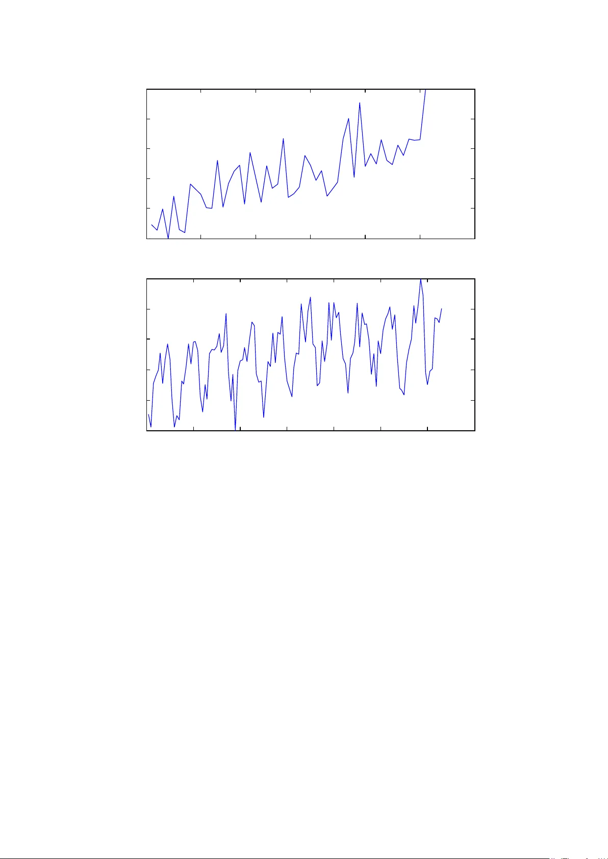
This is a preprint c opy that has been acce pted for publication in Neur ocomputing . Please cite this article as: T ao Xiong, Y ukun Bao, Zhongyi Hu, “Does Restraining End Ef fect Matter in EMD - Based Modeling Framework for T ime Series Prediction? Some Experime ntal Evidence s”. Neur ocomputing . 123, 2013: 174 - 184. Note: This prepri nt copy is only for perso nal use. I Resear ch Highlights • Propose EMD -based modeling framework with end condition methods • Slope- based and Rato’ s method are recommended w hen selecting end condition methods • Restraining the end ef fect improves the performance of EMD - based modeling framework D oes R estraining End Effect Matter in EMD -B ased Modeling F ramework for T ime Series Pr edict ion ? S ome E xperimental E vidences Tao Xiong, Yukun Bao * Department of Managem ent Science and Inform ation System s, , Zhongyi Hu School of Management , Huazhong Universit y of Science and Technology, Wuhan, P.R.China, 430074 Abstract F ollowing the “decomposition-and- ensemble ” principle, the empirical mode decomposition ( EMD )- based modeling framewor k has been widely used as a promising alternat ive for nonlinear and nonstationary time series modeling and prediction . T he end effect , w hich occurs during the sifting process of EMD a nd is apt to distort the decomposed sub- series and hurt the modeling process followed , however , has been ignored in previous studi es . Ad dressing the end ef fect issue, t his study proposes to incorporate end condition m ethods into EMD - based decomposition and ensemble modeling fram ework for one - and multi - step ahe ad time series predict ion . F our well - established end condition methods, Mirror method, Coughlin’ s method, Slope- based method , and Rato's method , are s elected , and support vector regression (S VR ) is employed as the modeling technique . For the purpose of just ification and comparison, well -known NN3 competition data se ts are used and four well - establ ished prediction models are selected as benchmarks. The experimental * Corresponding author : T el: + 86-27- 62559765; fax: +86 -27-87556437. Email: yukunbao@hust.edu.cn or y .bao@ieee.org results demonstrate d that significant im provement can be achieved by the proposed EMD - based SVR models with end condition methods . The EMD - SBM - SVR model and EMD - Rato - SVR mo del , in particu l a r, achieved the best prediction performances in terms of goodne ss of forecast measures and equality of accurac y of competing forecasts test . K eywords: E mpirical Mode Decomposition; End E ffect ; Support V ector Regression; E nsemble Modeling; T i me S eries Pr ediction. 1 1. I ntrodu ction T ime series modeling and predictio n is an area of enormous in terest s for both academics and prac titioners. The large num ber of studies have compared the forecast accuracies of alternative models based on statistical theories , suc h as autoregressive integrated moving average (ARIMA) [1] and autoregr essive conditional heteroskeda sticity (ARC H) [2] , or the ones based on computational intelligence, such as artificial ne ural networks (A NN) [3] and support vector regression ( SVR ) [4], for time series predic tion. E xisting research indicates that the lat ter emer ges the winner , especially i n short - term forecasting [5] . However , computational intelligence based forecasting models have their own shortcomings and disadvantages, e.g., local minima and over - fit ting in ANN models and sensitiveness to parameter selection in both SVR and ANN models. I n view of the lim itations for com putational intelligence based forecasting models, rec ently , a hybrid e mpirica l mode decomposition (EMD )-based m odeling framework introduced by Y u et al. [6 ] has estab lished itself as a promising alternative for nonlinear and nonstationary time series modeling and prediction . The attractiveness of the EMD - based modeling framework arises from the flexi ble decomposition-and- ensemble modeling structure res ulting in a simpl ifi cation of th e original com plicated mode ling task , and the employment of EMD with which any complex signals can be decomposed into a finite number of independent and nearly periodic intrinsic mode functions (IMFs) components and a residue based purely on the local characteristic tim e scale [7] . As such, EMD - based modeling fram ework has 2 been found to be a viable contender among various time - series models, e.g., autoregressive integrated moving average (ARIMA) [6, 8, 9], s easonal autoregressive i ntegrated moving a verage (SARIMA ) [ 10] , neural networks [9, 11 ], and support vector regression [12] , and successfully applied to different areas, including energy market [6, 11 - 13] , tourism management [9] , hydrology [14] , and t ransportation research [10], and emer gency managem ent [8] . Regarding to the end ef fect occurred during the sifting process of EMD , however , the research mentione d above (see [6 , 8-14] ) has paid little, even no attention to, which appeals this prese nt study . E nd eff ect is that when calcul ating the upper and lower envelops with cubic spline function in the sifting process of EMD , the divergence will appear on both ends of data series, and the diver gence gradually influ ences inside of da ta series so t ha t the results are distorted badly [15] , and always hurts the modeling quality as wel l as overall prediction performance when employing EMD - based decomposition and ensemble modeling fram ework for time series prediction. W ith regard to the problem of end eff ect, t here has been a vast and well - established bo dy of literature s on developing end condition method s for restraining the end ef fect. I n general, the end condition methods are essentially to use the known points to extend both beginning and end of the series by the addition of typical waves [7, 16] , extrema [ 17-20] , or predicted values [15, 21 , 22] . Although aforementioned st udies have clarif ied the capabili ty of these end condition methods on the restraining of end ef fect by means of, e.g., the orthogonality of IMFs [20] , th ere ha s been very few , if any , e f fort to evaluate the ef fectiveness of end c ondition methods in EMD - based modeling framework for 3 time series p rediction . So, we hope this study would fill this gap. In s ummary , The purpose of thi s study is to explicitly extend the E MD - based modeling framework with end condition methods for time series pr ediction , and then goes a step forward by providing the first expe rimental evidence within literature in which EMD - based model ing framework is applied for time series pred iction to justify wheth er restraining th e end ef fect is useful for achieving better prediction performance . If so, which end condition method dominate s ? For the purpose of justification , we conduct a larg e scale comparison study of EMD - based modeling framework incorporating selected end condition methods on the NN3 competition data. For the implementation of the proposed E MD -based modeling framework, support vector regression ( SVR ) is employed as modeling t echniq ue model in the current study in lights of that it has been found to be a viable contender am ong various time - series models [23-25] , and successfully applied to dif f erent areas [4, 26 , 27] . The paper unfolds as follows. Section 2 de scribe s r elated works about EMD, end ef fect , and end condition methods, indicating how end effect occurs and why it is important. The detail s on proposed procedure of EMD with end condition methods , support vector regression, and t he proposed EMD -based mod eling framework incorporating selected end condition methods are presented in Section 3 . Section 4 illustrates the research design on data source , preprocessing, selected c ounterparts, input selection, statistica l criteria , methodologies im plementation , and experimental procedure in details. Fol lowing that, in S ection 5, the experimental result s are 4 discussed. Finally , Section 6 summarizes and concludes this work. 2. Related works 2. 1 EMD and en d effect Empirical mode decomposition technique, first proposed by Huang et al . [7 ] , is a kind of adaptive signal decomposition technique using the Hilbert - Huang transform (HHT) and can be applied with nonlinear and nonstationary time series. Intrinsic - m ode functions (IMF) and the sifting process are the two key parts of the EMD technique . The term “intrins ic - mode function” is used be cause it represents the oscillation mode embedded in the data. An intri nsic - mode function is a function that sat isfies two conditions: ( 1 ) in the whole data serie s, the number of extrema (the sum of local maxima and local minima) and the number of zer o crossings must either be equal or differ at most by one; and ( 2 ) at any point, the mean value of the envelope defin ed by the local maxima and the envelope defined by the local minima is zero. W ith this definition, IM Fs can be extracted from the tim e series () xt according to the following sifting process: 1. Input time series () xt ; 2. Execute sifting process: (1) Initializ e : ( ) ( ) 0 r t xt = , and 1 i = ; (2) Extract the ith IMF: a. initializ e: ( ) ( ) 01 ,1 i ht r t k − = = ; b. Identify all of the extrema (maxima and minima) of ( ) 1 k ht − ; c . interpolate the local maxima and local minima by a c ubic spline to form upper and lower envelopes of ( ) 1 k ht − ; d . compute the mean ( ) 1 k mt − of the upper and lower envelopes just 5 establish ed; e . create: ( ) ( ) ( ) 11 kk k ht h t m t −− = − ; f . decide: if stopping criterion is satisfied then set ( ) ( ) IM F ki ht t = . Else return to step b, with 1 kk = + . (3) Define: ( ) ( ) ( ) 1 IM F ii i rt r t t − = − ; (4) If ( ) i rt is a constant or trend then sifting process can be stop, and the time series ( ) xt is decomposed into IMFs and residue, i.e., ( ) ( ) ( ) 1 = IM F i di d xt t r t = + ∑ . Else return to st ep (2), with 1 ii = + ; 3. Obtain fin al result, i.e. , the ( ) ( ) IM F , 1 d t ti ≤≤ , and the residue ( ) r i t . A s discussed in [21] , however , the two ends of the tim e series will disperse while the series is decomposed by EMD and this disperse , termed as end ef fect, would “empoison” in by the whole time series gradually mak ing the results to get distort ed . T o be more specific, e nd ef fect occurs during the sifting process, when the end points cannot be identified as the extrem a i n the procedure of 2 -(2)- b above , appealing specific measure to be taken to dea l with it. R ecently , a lar ge number of studies have develop ed end condition method s for restraining the end eff ect [7, 15-21] . Most of the proposed end condition methods are applied to “ add” the extrem a when end ef fect occurs, fa cilitating the construc tion of upper and lower envelopes during the sifting process of EMD. Details of four selec ted end condition methods in this study are presented in the following subsection 2. 2 End condition m ethods I n this study , we cannot examine all the end condition methods that might be useful in practice, and therefore w e consider various pr evious literat ures as guidance 6 and focus on the most commonly used end condition methods. F inally , selected end condition methods include the Mirror m ethod [17] , Coughlin ’ s method [16] , Slope- based method [19] , and Rato ’ s method [ 18 ] . For each selected end condition methods, there are a large num ber of variations proposed in the literature s , and it would be a hopeless task to consider all existing varieties. Our rule is the refore to consider the basic version of each method (without the additions, or the modifications proposed by some other researchers). D etailed discussions on the selected end condition methods can be found in [16-19] , but a brief introduction about their formulations is pr ovide d here. T o formulate the selected end condition methods , we adopt the notations and definitions in T able 1 . 1) Mirror me thod F or the beginning of time series () xt , a dd local mini mum (0) Min by mirror symmetry with respe ct to the local ma xi mum (1) Max ; for the end of ti me series () xt , add local maxi mum ( 1) Max n  by mirror symm etry with respect to the local maxi mum () Min n . The newly obtained (0) Min and ( 1) Max n  are then taken for construction of the upper and lower envelopes along with initial e xtrema . 2) Coughlin’ s method I n the Coughlin ’ s method, time series () xt is extend ed by additional typical waves defined as Eq . (1) instead of extrema employed in the mirror m ethod. W ave extension= 2 sin t A phase local me an P π  ++   . (1) 7 w here t he typical am plitude A and period P are determined by the following equations. ( ) ( ) ( ) (1) 1 , , 2 ( (1) ) ( (1) ) , 2 ( ( )) ( ( )) . begining end begining end A Max Min A Max n Min n P t Max t Mi n P t Max n t Min n = − = − = − = − (2) The addit ional typical w aves a re then taken for construction of the upper and lower envelopes along with initial series so that the additional waves are continually changing in amplitude and frequency . 3) Slope- based method F or the beginning of time series () xt , slope 1 s and 2 s are defined as Eq. ( 3 ) and Eq. (4 ) respectively .     21 1 ( ( 2)) ( ( 1 )) PQ s t Max t Mi n    (3)     11 2 ( (1) ) ( (1) ) QP s t Min t Max    (4) Then, the tim e gaps between the first tw o successive m a xima and minima are determined as   max 1 ( ( 2 )) ( ( 1 )) t t Ma x t Max   and   min 1 ( ( 2 )) ( ( 1 )) t t Mi n t Mi n   . The new extrema (0) Min and (0) Max are updated according to the corresponding time gaps   max 1 t  and   min 1 t  , and gradients 1 s and 2 s . The ordinate and abscissa of the new extrema are p ositioned at                 min max ( ( 0 )) ( ( 1 )) 1 ( ( 0 )) ( ( 1 )) 1 0 1 1 ( ( 1 )) ( (0 )) 0 0 2 ( (0) ) ( (0) ) t Mi n t Mi n t t Ma x t Max t Q P s t Ma x t Min P Q s t Mi n t Max         (5) 8 F or the end of time se ries, the sim ilar procedures are u sed to obtain ( 1) Max n  and ( 1) Min n  . The newly obtained (0) Min , (0) Max , ( 1) Min n  , and ( 1) Max n  are then taken for construction of the upper and lower envelopes along with initial extrema. 4) Rato ’ s method F or the beginning of () xt , assum e ( ) ( ) 10 tx = and ( ) ( ) ( ) ( ) 11 t Max t Min > . Add local minimum (0) Min , where ( 0 )= (1) Min Min , and ( ) ( ) ( ) ( ) 01 t Mi n t Max = − ; Add local maxi mu m (0) Max , where ( 0 )= (1) Max Max , and ( ) ( ) ( ) ( ) 01 t Max t Min = − . For the end of tim e series, the sim ilar procedures are used to obtain ( 1) Max n  and ( 1) Min n  . The newly obtained (0) Min , (0) Max , ( 1) Min n  , and ( 1) Max n  are then taken for construction of the upper and lower envelopes along with initial extrema. 3. Methodologies I n this sectio n, the overall formulation process of the proposed EMD - based SVR modeling framework is presented. F irst, EMD with end condition method is briefly introduced. Then a brief description of SVR algorithm is given. F inally , the proposed EMD - based SVR modeling f ramework i s formulated and the corresponding steps involved are presented in details. 3 .1 EMD with e nd c ondition m ethods Just as mentioned in Section 2.1, the sifting process is the key part of the EMD technique and e nd effect occurs during the sifting pr ocess, when the end points cannot be identified as the ex trem a, appealing end condition methods to be incorporated into 9 the sifting process. The improved sifting process with end condi tion method is depicted in Fi g.1. 3.2 Support vector re gression Support vector regression (SVR) , first propose d by V apnik et al. [28] based on the structured r isk minim ization princi ple, is found to be a viable contender among various time series models [4, 29] by m inimizing an upper bound of the generalization error . H ere, SVR is used as tool for foreca sting . T his subsection gives a brief description of SVR. The details of the formulation can be found in [28] . Given a set of data { } ( ) , 1, 2 , tt xy t T =  , where T t x ∈ℜ is the th t input pattern and t y is its corre sponding obs erved result, the basic idea of SVR is first to map the original data t x into a high - dimensional feature space via a nonlinear mapping function ( ) ϕ ⋅ , then to make linear regression in this high - dimension feature space and find the opti mal separating hype rplane with m inimal c lassification e rrors [12] . In general, SVR approximate the function using the following: ( ) ( ) T fx w x b ϕ = + (6) where ( ) x ϕ is the nonlinear function mapping from input space x into a high- dimensional feature space, and ( ) fx is the estimated value. C oef ficients T w and b are obtained by minimizing the regularized risk function, which can be transform ed into the following optimization problem: 10 ( ) ( ) ( ) ( ) ( ) ( ) * 1 * min 2 . . , 1, 2 , , , 1, 2 , , T T tt t T t tt T tt t ww st w x b y i T y w xb i T γ ζζ ϕ εζ ϕ εζ =  ++    +− ≤ + =   − + ≤+ =  ∑   １ (7) where γ is the penalty parameter , and nonnegative variables t ζ and * t ζ are the slack variables which repres ent the distances from actua l value to the corresponding boundary value of ε − tube. S o the problem of constructing the optimal hyperplane is t ransformed into the following the quadratic programming problem: ( ) ( ) ( ) ( ) ( ) ( ) ( ) ( ) [ ] * ** * , 11 1 1 ** 1 min 2 . . 0, , 0, nn n n i i j j i j ii ii aa ij i i n i i ii i a a a a x x ya ya st a a a a C φφ ε ε = = = =  − − ⋅ +− ++     −= ∈   ∑∑ ∑ ∑ ∑ (8) w here i a and * i a are corresponding Lagrange multipliers used to push and pull ( ) i fx towards the outcome of i y respectively . The decision function can be shown as: ( ) ( ) ( ) * 1 ,. xx n i i ij i fx a a K b = = −+ ∑ (9) ( ) ( ) ( ) ( ) , xx ij i j K xx φφ = ⋅ is defined as the kernel function. The elegance of using the kernel function is that one can deal with feature spaces of arbitrary dimensionality without having to compute the map ( ) x φ explicitly . I n this study , we select a common kernel function, i. e., RBF function, ( ) ( ) 2 , exp , 0 xx x x ij i j K γγ = −− > , as the kernel function. 3.3 T he proposed predic tion models It should be noted that SVR is employed as modeling technique in this study. As 11 such, this study turns out to develop different prediction models under EMD - based modeling framework with or without end condition m ethods using SVR , i.e., EMD - based SVR modeling framework for short. A s shown in Fig. 2 , th e proposed EMD - based SVR modeling framework is generally composed of the following three main steps: Step 1: The original series are first decomposed into a finite and often a small number of intrinsic mode functions (IMFs) and a residue us ing EMD technique. In the sifting process of EMD, selected end conditio n method is applied to restrain the end ef fect following the procedures illustrated in the above subsection. Step 2: After the components (IMF s and a residue) are adaptively extrac ted via EMD, each component is modeled by an independent SVR model to forec ast the component series respectively. Step 3: T he forecasts of all compone nts are aggregated using another independent SVR m odel, which model the relationship among the IMFs and the residue , to produce an ensem ble forecasts for the original se ries. Following the EMD - based SVR modeling framework, different prediction models can be developed. For exam ple, in case mirror method is selected a nd incorporated into the EMD to deal with end effect, t hen EMD - MM - SVR prediction model is derived . Following the same naming rule , EMD -Coughlin- SVR , EMD - SBM - SVR , and EMD - Rat o - SVR refer to the predic tion models w ith corresponding end condition methods respectively. It should be noted that EMD - SVR 12 refers to the model without any end condition methods. 4. Resear ch design This section provides details about the research desig n. I n s ection 4.1, the details of the data sets a nd relat ing data preprocessing proc edure are given. Section 4.2 presents the selected counterpa rts for comparison . T he input selection i s briefly presented in Section 4.3. Section 4.4 list s and briefly describes the goodness of forecast measures and equality of accuracy of competing forecasts tes t used . Section 4.5 presents the im plementation s of EMD , Wavelet , SVR , and SARIMA . Section 4. 6 depict s the experimental procedure s with NN3 com petition data in d etails . 4 .1 T he d ataset s and data p reprocessing The dataset s of 111 time series distributed for the NN3 competition are used for th is study 1 18 111 × . This competition was organized in 2007, and tar geted at computational intelligence based forecasting approaches . The data are monthly, with positive observations and structu ral characteristics which vary widely across the tim e series. Many of the series are dominated b y a strong seasonal structure ( e.g . #55, #57 and #73), while s ome series exhibit both trending and seasonal behavior (e.g. #1, #1 1 and #12). We leave the last 18 months of observations for evaluating a nd comparing the out-of- sample prediction performances of the proposed models against sel ected counterparts . All perform ance comparisons are based on these out of sample points. Since m ost of the time series considered exhibit strong seasonal component or 1 T he datasets can be obtained from http://www .neural -forecasting- competition .com/NN3/datas ets.htm 13 trend pattern as shown i n Fig.3, we c onduct deseasonalizing b y means of the revised multiplicative season al decomposition presente d in [30] . In addition, d etrending is performed by fitting a p olynom ial tim e trend and then subtracting the estim ated trend from the series when trends are detected by the Mann - Kendall test [31] . 4. 2 T he selected counterpa rts for comparis on Single SVR, Seasonal ARIMA (SA RIMA) and Wavele t- S VR [32] are selected as counterparts for the purpose of comparison. It should be noted the reason for selecting single SVR is to justify the effec tiveness of EMD - based m odeling framework, for the selection of SARIMA is due to the exhibited characteristics o f strong seasonality of the NN3 data sets, and for the selection of Wave let - SVR is the similar modeling mecha nism shared by EMD - based and Wavelet - based m odeling frameworks ( However, the present study focuses on the technical improvement on EMD - based modeling framework addressing the issue of end ef fect, but not the comparative study between EMD and W avelet though it could be an interesting topi c worthy of further exploration ). The essential form ulations of SARIMA and W avelet - SVR have been presented in many papers, so wi ll not be repeated here to keep this paper concise. For det ailed introduction to these methods, please refer to [10, 32]. Additionally , the perfo r mances on both o ne- step - ahead (prediction horizon H =1) and multi - step - ahead (prediction horizon H =18) predic tion are compared acros s all the models to provide more evidences for justifi cation. Note that th e iterated strategy 14 for multi - st ep - ahead prediction is employed in this study due to its simplicity and popularity in literature [11, 33] . This strategy construc ts a prediction m odel by means of minimizing the squares of the in - sample one - step - ahead re siduals, and then uses the predicte d value as an input for t he same model when we forecast the subs equent point, and continue in this manner until reaching the horizon. 4. 3 Input selection F ilter method is employed for input selection in this study. I n the case of the filter method, the best subset of inputs is selected a priori based only on the dataset. The input subs et is chosen by an evaluation criterion, which measures the relationsh ip of each subset of input variables with the output [34]. Specifically, in term s of evaluation criteria, th e partial mutual inform ation 2 35 [ ] is used for the prediction models. M utual information (MI) is a commonly adopted measure of dependence between variables and has bee n widely used for input selection [34] . H owever, this raises a major redund ancy i ssue redundancy issue because the MI criterion does not account for the interdependency between candi date variable. T o address this issue, Sharma [35 ] developed an improved algorithm that exploits the concept of partial mutual info rmation (P MI), which is the nonline ar stati stical analo g of partial correlation. The de fi nitions of PMI are shown as follows: ( ) ( ) ( ) ( ) '' '' '' , '' '' , , , ln XY XY XY f xy PMI f x y dx dy f xf y  =    ∫∫ (10) ' z x x Ex = −   ( 11 ) 2 The Matl ab code can be obtained from http://www .cs.tut.fi/~timhome/tim -1.0.2/tim/matlab/mutual_inform ation_p.m.htm 15 ' z y y Ey = −   (12) where ' X and ' Y are generalized to represen t time series () xt and lagged time () xt i − with tim e step i ( ) id ≤ conditional on Z which is a se t of rem aining time -lag variables. I n performing the PMI, the input variable that has the highest conditional PMI value at each iteration is add ed to the selection set. T he maximum embedding order d is set to 12 for the input selection process over al l the series from NN3 competition data sets [36] . 4.4 S tatisti cal criteria It should be noted that the impact of e nd condition methods on the quality of EMD has been widely i nvestigated in [7, 15-22] and it is not the focus of t he current study, but the impact of end condition methods on predi ction performance of E MD - based modeling framework for time series pred iction has not been widely explored which is the research goal of this study . H ence, statistical criteria such as goodne ss of forecast measur es (i.e., symmetric mean absolute percentage error (SMAPE) and mean absolute scaled error ( MASE ) ) and equality of accuracy of competing forecas ts test ( i.e., one- way analysis of variance (ANOV A) and T ukey honestly s ignifica nt d if ferenc e (HSD) test ) are employed here. T o compare the ef fectiveness of the dif ferent prediction models , no single accuracy measure can captur e all the distributional features of the errors when summarized across data series. Here, we consider tw o forecast accura cy measures. The first is the SMAPE defined as Eq. ( 13 ) , as this is the main measure cons idered in NN3 competition [37] . The second accuracy measure is the MASE, defined as Eq. 16 (14 ). It has recently been suggested by Hyndman and Koehler [38 ] as a means of overcoming observation and errors around zero existing in some measures. T he MASE has some feature s which are better than t he SMAPE, which has been criticized for the fact that i ts treatm ent of positive and negative erro rs is not sym metric [39] . H owever , because of its widespread use, the SMA PE will still be us ed in this stud y . The smaller the values of S MAPE and MASE, the closer are the predicted tim e series values to the actual values. ( ) 11 ˆ () () 1 SMA PE ˆ () () 2 MT mm mt mm xt xt MT xt xt = = − = ⋅ + ∑∑ (13) ( ) ( ) ( ) 11 2 ˆ () 1 M AS E 1 1 1 MT mm N mt mm i x t xt MT xi xi N = = =   − =  ⋅  −−  −  ∑∑ ∑ (14) w here () m xt denotes the observation at period t for time series m , ˆ () m xt denotes the forecast of () m xt , M is the number of tim e series (in this case, 111 M = ), T is the number of observation in the hold - out sample (in this case, 18 T = ), and N is the number of observa tion in the es timation sam ple for time serie s m . I n this study , we repeat running each model fifty tim es for NN3 dataset to even out the fluctuations . T hen each of the fift y runs wil l produce a SMAPE f or a l l 111 time series . Next, the mean and standard deviation of these fift y SMAPE a re calculated and listed in the tables for examining the performance of diff erent models . S imilarly , the mean and standard deviation of MASE are also com puted. N ote that the error measure s are computed after rolling back of the preprocessing step performed , such as deseasonalizatio n and detrending . 17 Following [40] , we also conduct a number of statistic al tests to compare each model based on the obtained fifty SMAPE and MASE at the 0.05 significance level. F or each prediction horizon ( 1 and 18 H = ) and performance measure (i.e., SMAPE and MASE) , we perform a one- way analysis of variance ( ANOV A ) procedure to determine if there exists statist ically significant dif ference among the eight models in out-of- sample forecasting. T hen, t o further identify the significant difference between any two mode ls , the T ukey honestly significant d ifference (HSD) test [41] is used to compare al l pairwise dif ferences simultaneously . Note that Tukey HSD test is a post- hoc test, this means that a researcher should not perform T ukey HSD test unl ess the results of ANOV A are positive. 4.5 M ethodologies i m plementation s In this study, E MD 3 Huang et al. [7 is implemented using the program provided by ] . T he number of sifting passes for IMF extraction is fixed at 10, and the w hole sifting process stops af te r 2 log N IMFs have been extracted, w here N is the lengt h of the data series . The W avelet toolbox in Matlab is used to implement the discrete W avelet transform . T his step involves several dif ferent families of Wa velet s and a detailed comparison of their performance. I n this study , the Daubechies ’ s W avelet s of order 7 is adopted through preliminary simulation in a trial - error fashi on . T o determine the number of decomposition levels , [ ] L int log( ) N = is used [ 42 ] . L presents the decomposition level while N denotes the length of the data series. 3 Matlab code are available at http: //rcada.ncu .edu.tw/ 18 LibSVM (version 2.86) 4 43 [ ] is e mployed for SVR modeling here . W e select t he Radial basis function (RBF) as the kernel function in the EMD - based prediction models when modeling the IMFs data. The linear kernel function is selected to model the relationship among the IMFs and the residue due to its simplicity and better performances after exte nsive experimental trials on diff erent kernel f unctions. To determine the hyper - parameters, nam ely ,, C εγ (in the case of R BF as the kernel function), a population - based search algorithm , nam ed p article swa rm optimiz ation (PSO) [44] , is employed in the curre nt study . D ue to its simplicity and gene rality as no important modification was made for applying it to model selection , PSO has been recen tly establish ed for parameter determination of SVR [45] . I n solving hyper- pa rameter selectio n by the PSO, each particle is requested to represent a potential solution ( ) ,, C εγ . Concerning the sele ction of p arameters (i. e., cognitive and interaction coefficients , swarm size, and number of iterations ) in binary P SO, it is yet anothe r challenging m odel selection task . Fortunately , several empirical and theoretical studies have been performed about the parameters of PSO from which valuable information can be obtained [46] . In this study, the parameters are determined according to the recommenda tions in these studies and sel ected based on the prediction performance and comp utational time in a trial - error fashion. Through experiment, the param eter values of PSO are se t as follows. B oth the cognitive and interaction coefficients are set to 2. The swarm size and number of iterations are s et to be 10 and 50 , respectively . 4 Matlab code are available at http://w ww .csie.ntu.edu.tw/~ cjlin/l ibsvm/ 19 For SA RIMA estimation, the automatic model selection algorithm proposed by Hyndman and Khandakar [47 ] and implemented in the R software pack age ‘forecast’ 5 It should be noted that in the m odel estimation stage for EMD - and W avelet -b ased SVR models, all the sa mples from training sets are decomposed at one time and used for model estimation. 10 fold cross validation is used for parameters tuning under the commonly used grid search. Finally , the achieved model based on training sets is tested on hold - out sample in the way as the decomposition is re peated with a next data added. is used in this study . 4.6 Experimenta l p rocedure Fig. 4 shows the procedure for performing experiments with the NN3 competition data in this study. Each series is split into the est ima tion sample and the hold- out sample firs tly . T hen, the optimal eight examined models for estim ation sample is determined. A f terwards, obtained eight models are used for one- a nd multi - step -ahead time series prediction for hold- out sample and the two accura cy measures are com puted. Furthermore, the modeling process for each series is repeated fifty times. Upon the termination of this loop, performance of the examined models is judged in terms of the mean and standard deviation of the SMAPE and MASE of fifty replications . I n addition, the ANOV A and Tu ke y HS D tests are used to tes t the statistical significance of a ny two competing prediction models at t he 0.05 significance level . 5 R package ‘forecast ’ are available at http://ftp.ctex.or g/mirrors/CRAN/ 20 5. R esults and di s cussions T he prediction performances of all the exam ined models (i.e., EMD - Rato - SVR, EMD -Coughlin- SVR, EMD - SBM - SVR, EMD - MM - SVR, EMD - SVR, W avelet - SVR, SVR, and SARIM A ) in terms of mean and standard deviation of two accuracy measures ( i.e., S MAPE and MASE) for one - and multi - step - ahead prediction are shown in Ta bl e 2 . As per the results presented, one can deduce the following observation:  O vera ll, t he proposed prediction models (these are, EMD - MM - SVR , EMD -Coughlin- SVR , EMD - SBM - SVR , and EMD - Rato - SVR ) outperform the EMD - based SVR pr edi ction model without any end condition methods (that is, EMD - SVR ) without exception . As such, we argue that the superior performance of proposed prediction models relative to EMD - SVR as a result of restraining the end effect occurred during the sifting p rocess of E MD .  T he proposed EMD - SBM - SVR and EMD - Ra to - SVR outperform the EMD - MM - SVR and EMD -Coughli n- SVR r egardless of the accuracy m easures and prediction horizon considered , indicating the supe riority of Slop e- based method and Rato’ s met ho d as end condition methods in EMD - based modeling framework from the perspective of time series prediction .  The six hybrid ensemble m odels (i.e., EMD - MM - SVR, EMD -Coughlin- S VR, EMD - SBM - SVR, EM D - Rato - SVR, EM D - SVR, and W avelet - SVR) consistently 21 achieve more accurate f orecast s than the two single models (i.e., SVR and SARIMA) . T he main reason could be that the decomposition strategy does ef fectively improve prediction performance.  A s f ar as the comparison between the EMD - SVR and W avelet - SVR , they are almost a tie and the resu lts are m ixing among the prediction measures and horizons e xamined. In terms of S MAPE, EM D - SVR wi ns for one - step - ahead prediction but loses for eighteen- step - ahead prediction. In terms of MA S E, EMD - SVR loses for one - step - ahead prediction but wins for eight een - ste p - ahead prediction .  W hen comparing single prediction m odels, the SARIMA model mostly ranks the last, while the SVR can produce fa r better resu lts. T he pos sible reason is that SARIMA is a typical linear model not sui table for capturing nonlinear pat ter ns hiding in the NN3 data set . F or each performanc e measure and prediction horizon, we perform an ANOV A procedure to determine if there exi sts statistica lly significa nt dif ference am ong the eight models in hold - out sample. T able 3 shows the results of AN O VA test, from which we can see that the all the A NOV A results are significant at the 0.05 significance level , sugg esting that there are significant d ifference s among the eight models. T o further identify the significant dif ference between any two m odels, the T ukey’ s HSD test is used to compare al l pairwise dif ferences simultaneously he re. T able 4 shows the results of these multip le comparison tests at 0.05 significance level ( for abbreviation, we use SBM , R ato, Coughlin, and MM in replace of 22 EMD - SBM - SVR, E MD - Rato - SVR, EMD -Coughlin- SVR, and EMD - MM - SVR respectively in this table ) . For each accuracy measure and prediction horizon, we rank order the models from 1 (the best) to 8 (the wors t). S everal observations can be made fro m T able 4 .  When considering one- step - ahead prediction, EMD - SBM - SVR and EMD - Rato - SVR significantly ou tperform the EMD - SVR across two measures .  H owever , when considering multi - step - ahead prediction, all the proposed four prediction models significantly outperform the EMD-S VR across two m easures.  T he EMD - SBM - SVR and EM D - Rato - SVR significantly outperform the EMD -Coughlin-S VR and EMD - MM - SVR , with on e exception, where EMD - MM - SVR performs the poor est at 95% st atistical con fidence level .  T here is no significant dif ference of prediction perform ance between EMD - SBM - SVR and EMD - Ra to - SVR . One exception occurs when 1 H = and SMAPE is used, in which the EMD - SBM - SVR significant ly outperform the EMD - Rato - SVR.  A s f ar as the comparison EMD - SVR vs. W avelet - SVR is concern ed, t he dif ference in prediction performance is not significant at the 0.05 level in all cases.  For each ac curacy measure and prediction horizon , the hybrid ensemble models significantly outperform the single models.  W hen comparing single prediction m odels , t he SVR performs significantly better than SARIMA without exception . 23  The SARIM A performs the poorest at 9 5 % statistic al confidence level in all cases . 6. C onclusions T his study contributed to propose an extension to well - establ ished EMD - based modeling framework by incorporating end condition methods for time series prediction , and provide lar ge sca le experimental evidences for the purpose of justification. T he experiment al results l ead to the following mai n conclusions. (1) T he original EM D - based modeling framewor k is outperformed by the propos ed four variants wi th differe nt end condition methods , confirming the helpfulness of restraining the end ef fect in the c ontext of time series modeling and prediction . (2) EMD - SBM - SVR and EMD - Rato - SVR achieved better as well as m ore stable prediction performances than the other counterparts in terms of rank - based m easure , indicat ing the superiority of slope-based method and Rato’ s method as end condition methods. T he limitations of this study lie in two aspects. F irs t , although we h ave examined a variety of end condition methods that are most co mmonly used in EMD literatures, there are many other possible methods in restraining the end effect o f EMD, which may shed a different light on the modeling issue. Second, F urth ermore, EEMD, recently proposed by W u and Huang [48 ] , is a substantial improvement over the original EMD, which may shed a different light on the modeling issue and further study to this regard is solic ited . 24 Acknowledgeme nt The authors would like to thank the anonymous reviewers for their valuable suggestions and constructive comments. This work was support ed by the Natural Science Foundation of China (Grant No. 70771042) and the Fundamental Research Funds for the Central Universities (2012QN208 - HUST) and a grant from the Modern Information Management Research Center at Huazhong University of Science and T echnology . 25 R eference [1] Y .S. Lee, L.I. T ong , Forecasting time series usin g a me thodology based on a utoreg ressive integrat ed mov ing avera ge and genet ic progra mmi ng. Knowl - based Syst 24 ( 2 0 11 ) 66 - 72. [2] C.W . Che ong , Mod eling and forecasting c rude oil markets u sing ARCH - type models . Ener g Poli cy 37 ( 2009 ) 2346 - 2355. [3] C.M. Le e, C.N. K o , T ime series prediction using RBF neural netw orks with a nonl inea r time - varying e volution PSO al gorithm . Neurocom putin g 73 ( 2009 ) 449 - 460. [4] K. Kim , Financial tim e serie s forecas ting usi ng suppo rt vect or machi nes. Neu rocomput ing 55 ( 2003 ) 307 - 319. [5] T . Hill, M. O'Connor , W . Remus , Neural Net work Models for T ime Series Forecasts. Manage Sci 42 ( 1996 ) 1082 - 1092. [6] L.A. Y u, S.Y . W ang, K.K. Lai , Forecasting crud e oil price with an EMD - based neural network ensem ble learn ing para digm . Ener gy Eco n 30 ( 2008 ) 2623 - 2635. [7] N.E. H uang, Z. Shen , S.R. Long, M. C. W u, H.H. Shih, Q. Zheng, et al. , The e mpir ical mode decompos ition and the Hi lbert s pectrum for nonli near an d non - stationary time series analysis. Proceedings of the Royal Society of London Series A: Mathematical, Physical and Engineering Sciences 45 4 ( 1998 ) 903 - 995. [8] X. Xu, Y . Qi, Z. Hua , Forecasting deman d of commodities after natural disasters. Expert Syst Appl 37 ( 2010 ) 4313 - 4317. [9] C.F . Chen, M.C . Lai, C.C . Y eh , Forecasting tourism dema nd based o n empi rical m ode decompos ition and neu ral netw ork. Knowl - based Syst 26 ( 2012 ) 281 - 287. [10] Y . W ei, M.C. Chen , Forecastin g the shor t - term met ro passenge r flow with e mpiri cal mode decompos ition and ne ural net works. T ransportati on Resea rch Par t C: Em er ging T echnolo gies 2 1 ( 2012 ) 148 - 162. [1 1] Z. Guo , W . Zhao, H. L u, J. W ang , Multi - step for ecasti ng for wi nd spee d using a modi fied EMD - based artificial neural networ k model. Renew Energ 37 ( 2012 ) 241 - 249. [12] L. T ang, L. Y u, S. W ang, J . Li, S. W ang , A novel hy brid ens emble learning paradigm for nucl ear ener gy c onsumpt ion forec asting . ApEn 93 ( 2012 ) 432 - 443. [13] Y . Dong, J. W ang, H. Jiang, J. W u , Short - term electricity price forecast based on the improv ed hybrid m odel. E ner g Conve rs Mana ge 52 ( 201 1 ) 2987 - 2995. [14] G . Napoli tano, F . Serina ldi, L. See , Impact of EMD decom positi on and random initia lisati on of weights in ANN hindcasting of daily stream flow series: An empirical examination. J Hydrol 406 ( 201 1 ) 199 - 214. [15] Y . Deng, W . W ang, C. Qian, Z. W ang, D. Dai , Boundary - pro cessing - technique in EMD m ethod a nd Hilbert transform. Chin Sci Bull 46 ( 2001 ) 954 - 960. [16] K. Cough lin, K.K. T ung , 11 - year solar cycle in the stratosphere extracted by the em pirical mode decompos ition m ethod. Adv Spa ce Res 34 ( 2004 ) 323 - 329. [17] G . Rilling , P . Flandrin, P . Gonçalvés , On empirical mode decomposition and its algorithms. IEEE- EURAS IP W orkshop on N onlinea r signa l and Im age Pro cessing ( 2003 ) 1- 5. [18] R. Rato, M. Ortigue ira, A. Batista , On the HHT , its problem s, and som e solut ions. Me ch Syst Signal Pr 22 ( 2008 ) 1374 - 1 394. [ 19] M. Dä tig, T . Schlurm ann , P erformance and limitations of the Hilbert – Huang tr ansform ation ( HHT) with an application to irregular water waves. OcEng 31 ( 2004 ) 1783 - 1834. [20] F . W u, L. Qu , An im proved m ethod fo r restra ining t he end ef fect in em pirical mode decom positi on and its applica tions t o the fa ult dia gnosis o f lar ge rot ating m achine ry . J So und V ib 314 ( 2008 ) 586 - 602. [21] J. Cheng, D. Y u, Y . Y ang , Applic ation of suppor t vector regress ion m achines to the proc essin g of end effects of Hilbert – Huang t ra nsform . Mech Syst Signal Pr 21 ( 2007 ) 11 9 7 - 1211. [22] D.C. Lin , Z.L. Guo, F .P . An, F . L. Zeng , Elimination of end effects in empirical mode decompos ition by mir ror image c oupled wi th supp ort vect or regress ion. M ech Syst S ignal Pr 31 ( 2012 ) 13 – 28. 26 [23] P .F . Pai, W .C. Hong , Suppo rt vector machines with simulated annealing algorithms in electricity load for ecastin g. Ener g Co nvers M anage 4 6 ( 2005 ) 2669 - 2688. [24] H. Pre m, N.R.S. R aghavan , A suppor t vector machine based approa ch for forecasting of network weather servic es. Journ al of Gri d Com puting 4 ( 2006 ) 89 - 11 4 . [25] K.Y . Che n, C.H. W ang , Support ve ctor regression with genetic algorith ms in forecasting tourism demand. T ourism Management 28 ( 2007 ) 215 - 226. [26] P .S. Y u, S.T . Chen, I. F . Chang , Support vector re gr ession for real - time flood stag e forecasting. J Hydrol 328 ( 2006 ) 704 - 716. [27] D. Niu, D. Liu, D.D. W u , A soft com puting sy stem for day - ahead electricity price forecasting. Applied S oft Com puting 10 ( 2010 ) 868 - 875. [28] V . V apnik, S.E. G olowich, A. Smola , Suppo rt vecto r met hod for fu nction a pproxim ation, regressi on esti mati on, and si gnal proc essing . Advanc es in neu ral inf ormat ion proce ssing sys tems ( 1997 ) 281 - 287. [29] Q. Li, Q. Meng , J. Cai, H. Y oshin o, A. Mochida , Applying su pport vect or m achine t o pred ict hourly cooling l oad in the bui lding. ApEn 86 ( 2009 ) 2249 - 225 6. [30] R.R. Andra wis, A.F . Atiya, H. El - Shis hiny , Forecast combinations of computation al intelligence and linear models for the NN5 tim e series forecasting competition. Int J Forecasting 27 ( 201 1 ) 672 - 688. [31] B. Onoz , M. Bayazit , The power of statistical tests fo r trend detection. T urkish Journal of Engineeri ng an d Enviro nment al Scienc es 27 ( 2003 ) 247 - 251. [32] O. Kisi, M. Cimen , Precipitation fore casting by using wavelet - support vector mach ine conjunction model. Eng Appl Ar tif I ntel 25 ( 2012 ) 783 - 792. [33] L. T ang, L. Y u, S. W ang, J . Li, S. W ang , A novel hy brid ens emble learning paradigm for nucl ear ener gy cons umption foreca sting. ApEn 93 ( 201 1 ) 432 - 443. [34] A. Sorja maa, J. Hao, N. Reyh ani, Y . Ji, A. Lendasse , Methodol ogy for lo ng - term p redi ction o f time series. N eurocom puting 7 0 ( 2007 ) 286 1 - 2869. [35] A. S harma , Seasonal to intera nnual ra infall probabi listic forecast s for im proved wate r suppl y management: Part 1 — A strategy f or syst em predi c tor identification. J Hydrol 239 ( 2000 ) 232 - 239. [36] S. Be n T aieb, A. Sorjam aa, G . Bontem pi , Multiple - output model ing fo r multi - step - ahead time series forecasting. Neurocomputing 73 ( 2010 ) 19 50 - 1957. [37] S.F . Crone, K. Nikolopoul os, M. Hi bon , Autom atic Modelling and For ecasting with Artificial Neural Networks – A forecasti ng com petiti on evaluat ion. I IF/SAS Gra nt 20 05 Resea rch Re port 200 8 ) . [38] R.J. Hynd man, A.B. Koehle r , Another look at measures of forecast accuracy . Int J Forecasting 22 ( 2006 ) 679 - 688. [3 9] P . Goodwin, R. Lawton , On the asymmetry of th e symmetric MAPE. Int J Forecasting 15 ( 1999 ) 405 - 408. [40] M. Qi, G .P . Zhang , Tr e n d t i m e – series model ing and fo recasti ng wit h neural ne twork s. Neural Networks , IEE E T ransactio ns on 19 ( 2008 ) 808 - 816. [41] B. T ukey’ s , Multip le comparisons. ( 1953 ) . [42] V . Nourani, M.T . Alami, M.H. Am infar , A combined ne ural - wavelet model for prediction of Ligvanc hai wate rshed preci pitat ion. Eng Appl Artif Int el 22 ( 2009 ) 466 - 472. [43] C.C. Cha ng, C.J. Li n , LIBSVM: a libr ary for support vector machines. ACM T ran sactions on Intelligen t Systems and T echnology ( TIST) 2 ( 2011 ) 27. [44] R.C. Eberhart, Y . Shi, J. Kennedy . Swarm intelligence: Else vier; 2001. [45] X. Guo, J. Y ang, C. W u, C. W ang, Y . Liang , A novel L S - SVMs hyper - par ame te r selection based on particl e swarm optim ization. Neurocom puting 71 ( 2008 ) 321 1 - 3215. [46] J. F . Kennedy , J. Kennedy , R.C. Ebe rhart. Swarm intell igence: M or gan Kauf mann Pu b; 2001 . [47] R.J. Hy ndman, Y . Khanda kar , Automatic T ime Series for Forecasting: The Forecast Package for R. journal of statistical software 26 ( 2007 ) 1- 22. [48] Z. W u, N.E. Huang , Ensemble em pirical mode de compos ition: A noise - assisted data analysis method. Advance s in Adapti ve Data Analys is 1 ( 2 009 ) 1- 41. Captio n page T able 1: Notation and definition for end condition methods T able 2: Prediction accuracy measure of dif ferent models for hold -out sample Ta bl e 3: ANOV A results for hold - out ample Ta bl e 4: T ukey HSD test results with ranked models for hol d-out sample Fig . 1: The EMD with end condition method Fig. 2: The EMD - based SV R modeling f ramework Fig. 3: T wo representative NN3 time series (#12 and #55) Fig. 4: Experiment procedures Figur es Input time series Identify all of the extrema of Initialize ( ) ( ) 0 ,1 r t xt i = = Initialize ( ) ( ) 01 ,1 i ht r t k − = = ( ) 1 k ht − Apply end condition method to extend ( ) 1 k ht − Create the upper and lower envelopes of extended ( ) 1 k ht − Compute the ( ) 1 k mt − Create ( ) ( ) ( ) 11 kk k ht h t m t −− = − Stopping criterion is satisfied 1 kk = + No Yes ( ) ( ) IMF ki ht t = Define ( ) ( ) ( ) 1 IMF ii i rt r t t − = − is a constant or trend ( ) i rt Yes 1 ii = + No ( ) ( ) ( ) 1 = IMF i di d xt t r t = + ∑ Extract the ith IMFs Execute sifting process ( ) xt Start End Fig. 1. The E MD with end condition m ethod EMD with end condition method …… SVR 1 SVR 2 SVR n+1 SVR n …… …… SVR Input Output Step 1 Step 2 Step 3 Original time series IMF 1 IMF 2 IMFn R n Prediction results of IMF 1 Prediction results of IMF 2 Prediction results of IMF n Prediction results of R n Final prediction results Fig . 2 The EMD - based SV R modeling fra mework 0 10 20 30 40 50 60 0 0. 2 0. 4 0. 6 0. 8 1 Ti m e Ti m e S eries #12 0 20 40 60 80 100 120 140 0 0. 2 0. 4 0. 6 0. 8 1 Ti m e Ti m e S eries #55 Fig. 3. T wo representative NN3 tim e series (#12 a nd #55) Start Split series into estimation sample and hold-out sample Predict time series using Calculate SMAPE and MASE Repeated 50 times? Calculate the mean and standard deviation of each accuracy measure End Yes No Perform ANOVA and Tukey HSD test Input time series > 111 j Yes No = +1 jj th j Compare the quality of obtained results 1 j = SARIMA SVR Wavelet- SVR EMD-SVR EMD-MM- SVR EMD-SBM- SVR EMD- Coughlin-SVR EMD-Rato- SVR Fig. 4 . Experiment proc edures T ables T able 1 Notation and definition for en d condition m ethods Notation Definition () xt T he input t ime ser ies , ( ) { ( 1 ), ( )} x t x xT =  i I ndex of local max imu m , 1, , in =  j I ndex of local min imu m , 1, , jm =  (1) Max , (1) Min F irst two local extrema of ti me series () xt () Max n , () Min m Last two local extr ema of time s eries () xt () Pi O rdinate value of () Max i respectively () Qj O rdinate value of () Min j respectively ( ( )) t xt T ime index of () xt ( ( )) t Max i T ime index of () Max i ( ( )) t Min j T ime index of () Min j () max ti ∆ T ime gaps be tween two suc cessive loc al m axima, ( ) ( ( 1 )) ( ( )) max t i t Max i t Max i ∆ = +− () min tj ∆ T ime gaps be tween two suc cessive local minima, ( ) ( ( 1 )) ( ( )) min t j t Min j t Min j ∆ = +− T able 2 Pr ediction accuracy measure of dif ferent models for hold - out sample P rediction hor izon M odel SMAPE MAS E Mean Std Mean Std 1 H = EMD - Rato - SVR 7.854 0.0 2 64 0.8 87 0.00 26 EMD - Coughlin - SVR 10.84 5 0.0315 0.9 56 0.00 31 EMD - SBM - SVR 6. 4 94 0.0305 0.8 34 0.00 29 EMD - MM - SVR 1 1.084 0 .0278 0.9 45 0.0025 EMD - SVR 1 1.201 0.0295 1.0 06 0.0041 W avelet - SVR 12.012 0.03 06 0.984 0.0037 SVR 13.854 0.0297 1. 11 3 0.0057 SARIMA 17.125 0. 00 01 1. 231 0.000 0 18 H = EMD - Rato - SVR 16.274 0.0321 1.1 87 0.0034 EMD - Coughlin - SVR 18.00 5 0.0307 1.214 0 .0065 EMD - SBM - SVR 16.094 0 .0285 1.1 96 0.0048 EMD - MM - SVR 18.264 0.03 12 1.424 0.0032 EMD - SVR 20.241 0.0348 1.580 0 .0047 W avelet - SVR 19.594 0.03 71 1.612 0.0052 SVR 22.254 0.0315 1.802 0 .0038 SARIMA 24.854 0.000 1 2.216 0.000 0 T able 3 ANOV A result s for hold - out ample Prediction hor izo n Measure ANOV A T est Statis tics F p- value 1 H = SMAPE 29.815 0.000 * MASE 18.497 0.000 * 18 H = SMAPE 9.640 0.001 * MASE 25.874 0.000 * Notes: * indicates the mean differ ence among the eight models is signif icant a t the 0.05 level. T able 4 T u key HSD test results with ra nked model s for hold - ou t sample P rediction horizon M easure Ranks of m odels 1 2 3 4 5 6 7 8 1 H = SMAPE SBM <* Rato <* Coughlin < MM < EMD - SVR < W avelet - SVR <* SVR <* SARIMA MASE SBM < Rato < MM < Coughlin < W avelet - SVR < EMD - SVR <* SVR <* SARIMA 18 H = SMAPE SBM < Rato <* Coughlin < MM <* W avelet - SVR < EMD - SVR <* SVR <* SARIMA MASE Rato < SBM < Coughlin <* MM <* EMD - SVR < W avelet - SVR <* SVR <* SARIMA Notes: * indi cates the mean dif ference b e tween the two adjac ent models is significant at the 0.05 le vel . ‘ SBM ’ corre sponds to the EMD - SBM - SVR model, ‘ Rat o ’ corresponds to the EMD -Rato- SVR model, ‘Coughlin ’ corresponds to the EMD -Coughlin- SVR model, and ‘ MM ’ corresponds to the EMD - MM - SVR model.