Sparse Recovery with Very Sparse Compressed Counting

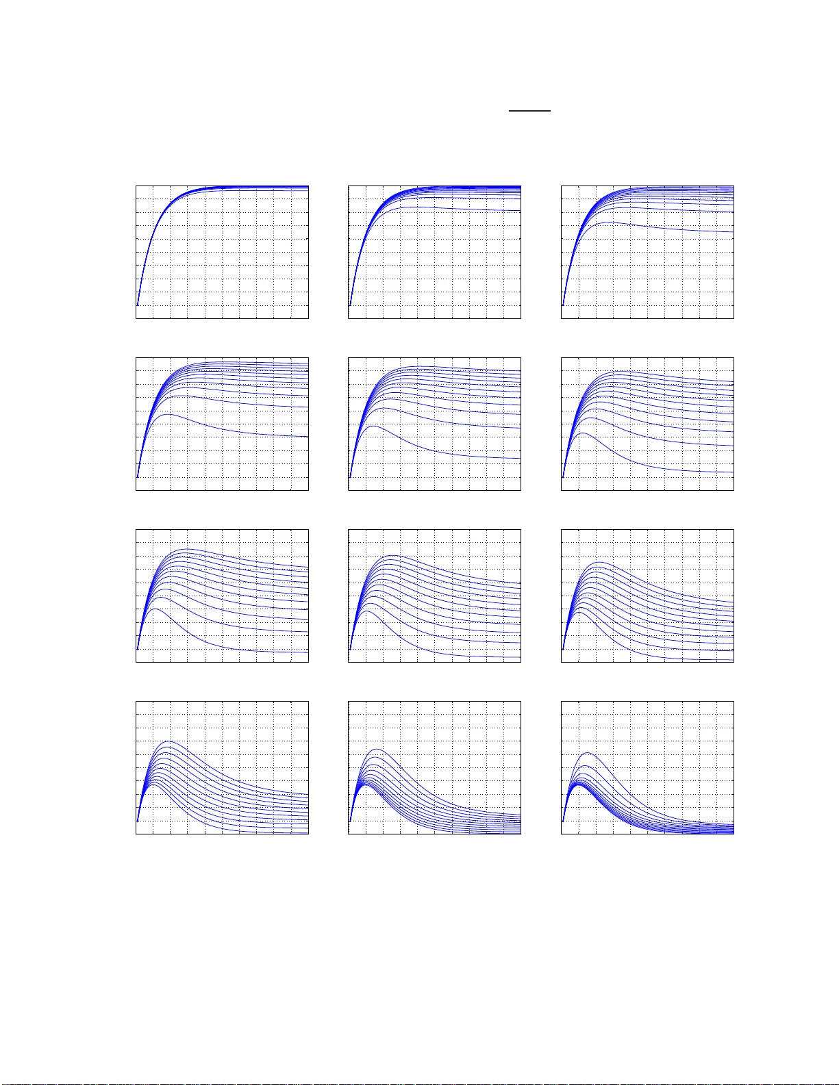
Sparse Recov ery with V ery Sparse Compressed Counting Ping Li Department of Statistics & Biostatist ics Department of Computer Science Rutgers Univ ersity Piscataw ay , NJ 08854, USA pingli@sta t.rutgers. edu Cun-Hui Zhang Department of Statistics & Biostatistics Rutgers Univ ersity Piscataw ay , NJ 08854, USA czhang@sta t.rutgers. edu T ong Zhang Department of Statistics & Biostatist ics Rutgers Univ ersity Piscataw ay , NJ 08854, USA tongz@rci. rutgers.ed u Abstract Compressed 1 sensing (sparse signal recovery) often encounters nonnegative data (e.g., imag es). Recently [11] d ev eloped the meth odolog y of using (d ense) Compr essed Cou nting for recovering nonnegativ e K - sparse signals. In this paper, we ado pt ve ry sparse Comp r e ssed Counting for no nnegative signal recovery . Our design matrix is sam pled from a maximally -ske wed α -stable distrib ution ( 0 < α < 1 ), and we spar - sify the design m atrix so that on average (1 − γ ) -fraction of the en tries become zero . Th e idea is r elated to very sparse sta ble rando m pr o jections [9, 6 ], the prior work f or estimating summary statistics of the data. In our the oretical analy sis, we show that, when α → 0 , it suffices to use M = K 1 − e − γ K log N /δ mea- surements, so that wit h probability 1 − δ , all coordina tes can be recovered within ǫ add itiv e precision, in one scan of the coo rdinates. I f γ = 1 (i.e ., dense design), then M = K log N /δ . If γ = 1 / K or 2 /K (i.e., v ery spar se design), then M = 1 . 58 K log N /δ or M = 1 . 16 K log N /δ . This means the design matrix can be indeed very sparse at only a minor inflation of the sample complexity . Interestingly , as α → 1 , the required number o f measurements is essentially M = eK log N /δ provided γ = 1 /K . It turn s out that this complexity eK log N /δ (at γ = 1 /K ) is a general worst-case bound. 1 Part of the conten t of this paper was sub mitted t o a conferen ce in May 2013 . 1 1 Introd uction In a recent paper [11], we de velop ed a ne w frame work for compresse d sensing (sparse signal recov ery) [4, 2], by focusing o n n onne gati ve s parse signals, i.e., x ∈ R N and x i ≥ 0 , ∀ i . Note that re al-world signals a re often nonne gati ve. The technique was based on Compr essed Counting (CC) [8, 7, 10]. In that f ramew ork, entries of the (dense) design matrix are sampled i.i.d. from an α -stable ma ximally-sk e wed dis trib ution. In this paper , we in tegra te the idea of ver y spar se stable r andom pr oje ctions [9, 6] in to the proce dure, to de- vel op very sparse compr essed counting for compr essed sensing . In this paper , our procedure for compressed sensing first collects M non-adap tiv e li near measurement s y j = N X i =1 x i [ s ij r ij ] , j = 1 , 2 , ..., M (1) Here, s ij is the ( i, j ) -th entry of the de sign matrix with s ij ∼ S ( α, 1 , 1) i.i.d, where S ( α, 1 , 1) deno tes an α -stabl e maximally-sk ewed (i.e., sk e wness = 1) distr ibu tion with unit scale . Instead of usin g a dense desig n matrix, we randomly sparsif y (1 − γ ) -fract ion of the entries of the design matrix to be zero, i.e., r ij =  1 with prob . γ 0 with prob . 1 − γ i.i.d. (2) And an y s ij and r ij are also indepe ndent. In the decod ing phase, our proposed estimator of the i -th coordina te x i is simply ˆ x i,min,γ = min j ∈ T i y j s ij r ij (3) where T i is the set of nonz ero entries in the i -th row of the desi gn m atrix, i.e., T i = { j, 1 ≤ j ≤ M , r ij = 1 } (4) Note that the size of the set | T i | ∼ B inomial ( M , γ ) . T o a nalyze the sample comple xity (i.e., the requi red number of measur ements), we need to study the follo wing error probability Pr ( ˆ x i,min,γ > x i + ǫ ) (5) from which we can deri ve the sample complexit y by using the follo w ing inequalit y N Pr ( ˆ x i,min,γ > x i + ǫ ) ≤ δ (6) so that any x i can be estimated within ( x i , x i + ǫ ) with a probabi lity (at least) 1 − δ . Main Result 1 : As α → 0 + , the required number of measurements is M = 1 − log h 1 − 1 K +1 (1 − (1 − γ ) K +1 ) i log N /δ (7) which can essenti ally be w ritten as M = K 1 − e − γ K log N/δ (8) 2 If γ = 1 /K , then the required M is about 1 . 58 K log N/δ . If γ = 2 /K , then M is about 1 . 16 K log N /δ . In other words, we can use a very sparse design matrix and the required number of m easure ments w ill only be inflated slight ly , if we choose to use a small α . Indeed , using α → 0+ achie ves the smallest complexity . Howe ver , there will be a numerical issue if α is too small. T o see this, consider the ap proximate mechanism for genera ting S ( α, 1 , 1) by using 1 /U 1 /α , where U ∼ unif (0 , 1) . If α = 0 . 05 , then we ha ve to compute (1 /U ) 20 , which may potent ially create nu- merical problems. In our Matlab simulations, we do not notice obvious numerical issues w ith α = 0 . 05 (or e ven smaller). H o wev er , if a devic e (e.g., camera or other hand-held devic e) has a limited precisio n and/or memory , then we exp ect that we must use a large r α , away from 0. Main Result 2 : If x i > ǫ whene ver x i > 0 , then as α → 1 − , the requir ed number of measuremen ts is M = 1 − log  1 − 1 K +1  1 − 1 K +1  K  log N/δ, with γ = 1 K + 1 (9) This comple xity bound can essentially be written as M = eK log N /δ, with γ = 1 K (10) Interes tingly , this result eK log N/δ (w ith γ = 1 /K ) is the general worse-ca se bound. 2 A Simulation Study W e 2 consid er two types of signals. T o generate “binary signal”, we randomly select K (out of N ) coordi- nates to be 1. For “non-bin ary signal”, w e assign the va lues of K randomly selected nonzero coordinat es accord ing to | N (0 , 5 2 ) | . T he number of measure ments is determined by M = ν K log N /δ (11) where N ∈ { 10000 , 100000 } , δ = 0 . 01 and ν ∈ { 1 . 2 , 1 . 6 , 2 } . W e report the normalized reco very errors: Normalized Error = s P N i =1 ( x i − estimated x i ) 2 P N i =1 x 2 i (12) W e expe riment with all possible val ues of 1 /γ ∈ { 1 , 2 , 3 , ..., K } , although w e only plot a few selected γ v alues in Figures 1 t o 4. For ea ch combi nation ( γ , N , ν ) , we con duct 100 s imulations and r eport the median errors. The results confirm our theoretica l analysi s. When ν is small (i.e., less measurements), w e need to choos e a small α in order to achie ve perfect recove ry . When ν is lar ge (i.e., more measurement s), we can use a lar ger α . Also, the simulation s confirm that, in general , we can choose a very spa rse design. 2 This report does not includ e comparisons with the SMP algorithm [1, 5], as we can no t run the code from http://groups .csail.mit.ed u/toc/sparse/wiki/index.php?title=Sparse_Recovery_Experiments , at the moment. W e will provide the comparisons after we are able to execute t he code. W e thank the communications with the author of [1, 5]. 3 0 0.2 0.4 0.6 0.8 1 0 0.05 0.1 0.15 0.2 1/ γ = 1 N = 10000, K = 10, ν = 1.2 Binary Signal 1/ γ = 5 1/ γ = 10 α Normalized error 0 0.2 0.4 0.6 0.8 1 0 0.05 0.1 0.15 0.2 1/ γ = 1 N = 10000, K = 10, ν = 1.2 Non−Binary Signal 1/ γ = 5 1/ γ = 10 α Normalized error 0 0.2 0.4 0.6 0.8 1 0 0.05 0.1 0.15 0.2 1/ γ = 1 N = 10000, K = 10, ν = 1.6 Binary Signal 1/ γ = 5 1/ γ = 10 α Normalized error 0 0.2 0.4 0.6 0.8 1 0 0.05 0.1 0.15 0.2 1/ γ = 1 N = 10000, K = 10, ν = 1.6 Non−Binary Signal 1/ γ = 5 1/ γ = 10 α Normalized error 0 0.2 0.4 0.6 0.8 1 0 0.05 0.1 0.15 0.2 1/ γ = 1 N = 10000, K = 10, ν = 2 Binary Signal 1/ γ = 5 1/ γ = 10 α Normalized error 0 0.2 0.4 0.6 0.8 1 0 0.05 0.1 0.15 0.2 1/ γ = 1 N = 10000, K = 10, ν = 2 Non−Binary Signal 1/ γ = 5 1/ γ = 10 α Normalized error Figure 1: Normalized estimation errors (12) with N = 10000 and K = 10 . 4 0 0.2 0.4 0.6 0.8 1 0 0.05 0.1 0.15 0.2 1/ γ = 1 N = 10000, K = 20, ν = 1.2 Binary Signal 1/ γ = 5 1/ γ = 10 1/ γ = 20 α Normalized error 0 0.2 0.4 0.6 0.8 1 0 0.05 0.1 0.15 0.2 1/ γ = 1 N = 10000, K = 20, ν = 1.2 Non−Binary Signal 1/ γ = 5 1/ γ = 10 1/ γ = 20 α Normalized error 0 0.2 0.4 0.6 0.8 1 0 0.05 0.1 0.15 0.2 1/ γ = 1 N = 10000, K = 20, ν = 1.6 Binary Signal 1/ γ = 5 1/ γ = 10 1/ γ = 20 α Normalized error 0 0.2 0.4 0.6 0.8 1 0 0.05 0.1 0.15 0.2 1/ γ = 1 N = 10000, K = 20, ν = 1.6 Non−Binary Signal 1/ γ = 5 1/ γ = 10 1/ γ = 20 α Normalized error 0 0.2 0.4 0.6 0.8 1 0 0.05 0.1 0.15 0.2 1/ γ = 1 N = 10000, K = 20, ν = 2 Binary Signal 1/ γ = 5 1/ γ = 10 1/ γ = 20 α Normalized error 0 0.2 0.4 0.6 0.8 1 0 0.05 0.1 0.15 0.2 1/ γ = 1 N = 10000, K = 20, ν = 2 Non−Binary Signal 1/ γ = 5 1/ γ = 10 1/ γ = 20 α Normalized error Figure 2: Normalized estimation errors (12) with N = 10000 and K = 20 . 5 0 0.2 0.4 0.6 0.8 1 0 0.05 0.1 0.15 0.2 1/ γ = 1 N = 10000, K = 100, ν = 1.2 Binary Signal 1/ γ = 25 1/ γ = 50 1/ γ = 100 α Normalized error 0 0.2 0.4 0.6 0.8 1 0 0.05 0.1 0.15 0.2 1/ γ = 1 N = 10000, K = 100, ν = 1.2 Non−Binary Signal 1/ γ = 25 1/ γ = 50 1/ γ = 100 α Normalized error 0 0.2 0.4 0.6 0.8 1 0 0.05 0.1 0.15 0.2 1/ γ = 1 N = 10000, K = 100, ν = 1.6 Binary Signal 1/ γ = 25 1/ γ = 50 1/ γ = 100 α Normalized error 0 0.2 0.4 0.6 0.8 1 0 0.05 0.1 0.15 0.2 1/ γ = 1 N = 10000, K = 100, ν = 1.6 Non−Binary Signal 1/ γ = 25 1/ γ = 50 1/ γ = 100 α Normalized error 0 0.2 0.4 0.6 0.8 1 0 0.05 0.1 0.15 0.2 1/ γ = 1 N = 10000, K = 100, ν = 2 Binary Signal 1/ γ = 25 1/ γ = 50 1/ γ = 100 α Normalized error 0 0.2 0.4 0.6 0.8 1 0 0.05 0.1 0.15 0.2 1/ γ = 1 N = 10000, K = 100, ν = 2 Non−Binary Signal 1/ γ = 25 1/ γ = 50 1/ γ = 100 α Normalized error Figure 3: Normalized estimation errors (12) with N = 10000 and K = 100 . 6 0 0.2 0.4 0.6 0.8 1 0 0.05 0.1 0.15 0.2 1/ γ = 1 N = 100000, K = 10, ν = 2 Binary Signal 1/ γ = 5 1/ γ = 10 α Normalized error 0 0.2 0.4 0.6 0.8 1 0 0.05 0.1 0.15 0.2 1/ γ = 1 N = 100000, K = 10, ν = 2 Non−Binary Signal 1/ γ = 5 1/ γ = 10 α Normalized error 0 0.2 0.4 0.6 0.8 1 0 0.05 0.1 0.15 0.2 1/ γ = 1 N = 100000, K = 20, ν = 2 Binary Signal 1/ γ = 5 1/ γ = 10, 20 α Normalized error 0 0.2 0.4 0.6 0.8 1 0 0.05 0.1 0.15 0.2 1/ γ = 1 N = 100000, K = 20, ν = 2 Non−Binary Signal 1/ γ = 5 1/ γ = 10 1/ γ = 20 α Normalized error 0 0.2 0.4 0.6 0.8 1 0 0.05 0.1 0.15 0.2 1/ γ = 1 N = 100000, K = 100, ν = 2 Binary Signal 1/ γ = 25 1/ γ = 50, 100 α Normalized error 0 0.2 0.4 0.6 0.8 1 0 0.05 0.1 0.15 0.2 1/ γ = 1 N = 100000, K = 100, ν = 2 Non−Binary Signal 1/ γ = 25 1/ γ = 50 1/ γ = 100 α Normalized error Figure 4: Normalized estimation errors (12) with N = 10000 0 and ν = 2 . 7 3 Analysis Recall, we colle ct our measur ements as y j = N X i =1 x i s ij r ij , j = 1 , 2 , ..., M (13) where s ij ∼ S ( α, 1 , 1) i.i.d. and r ij =  1 with prob . γ 0 with prob . 1 − γ i.i.d. (14) And an y s ij and r ij are also indepe ndent. Our propose d estimator is simply ˆ x i,min,γ = min j ∈ T i y j s ij r ij (15) where T i is the set of nonz ero entries in the i -th row of S , i.e., T i = { j, 1 ≤ j ≤ M , r ij = 1 } (16) Conditio nal on r ij = 1 , y j s ij r ij     r ij = 1 = P N t =1 x t s tj r tj s ij = x i + P N t 6 = i x t s tj r tj s ij = x i + ( η ij ) 1 /α S 2 S 1 (17) where S 1 , S 2 ∼ S ( α, 1 , 1) , i.i.d., and η ij = N X t 6 = i ( x t r tj ) α = N X t 6 = i x α t r tj (18) Note that E ( η ij ) = γ N X t 6 = i x α tj ≤ γ N X t =1 x α tj , lim α → 0+ E ( η ij ) ≤ γ K (19) When the signals are binary , i.e., x i ∈ { 0 , 1 } , we ha ve η ij ∼  B inomial ( K, γ ) if x i = 0 B inomial ( K − 1 , γ ) if x i = 1 (20) The key in our theoret ical analysis is the distrib ution of the ratio of two indepen dent stab le rando m v ariables . H ere, we consi der S 1 , S 2 ∼ S ( α, 1 , 1) , i.i.d., and define F α ( t ) = Pr  ( S 2 /S 1 ) α/ (1 − α ) ≤ t  , t ≥ 0 (21) There is a standar d proced ure to sample from S ( α, 1 , 1) [3]. W e first generate an expone ntial random v ariable with mean 1, w ∼ exp(1) , and a uniform random va riable u ∼ un if (0 , π ) , and then compute sin ( αu ) [sin u cos ( απ / 2)] 1 α  sin ( u − αu ) w  1 − α α ∼ S ( α, 1 , 1) (22) 8 Lemma 1 [11] F or any t ≥ 0 , S 1 , S 2 ∼ S ( α, 1 , 1) , i.i.d., F α ( t ) = Pr  ( S 2 /S 1 ) α/ (1 − α ) ≤ t  = 1 π 2 Z π 0 Z π 0 1 1 + Q α /t du 1 du 2 (23) wher e Q α =  sin ( αu 2 ) sin ( αu 1 )  α/ (1 − α )  sin u 1 sin u 2  1 1 − α sin ( u 2 − αu 2 ) sin ( u 1 − αu 1 ) (24) In parti cular , lim α → 0+ F α ( t ) = 1 1 + 1 /t , F 0 . 5 ( t ) = 2 π tan − 1 √ t  (25) 3.1 Err or Probability The follo wing Lemma deriv es the general formula (26 ) for the error probabi lity in terms of an exp ectation , which in genera l does not hav e a close-f orm solution. Neve rtheless , when α = 0+ and α = 0 . 5 , we can deri ve two con veni ent upper bounds, (28) and (30), respecti vely , w hich ho we ver are not tight. Lemma 2 Pr ( ˆ x i,min,γ > x i + ǫ ) = " 1 − γ E ( F α  ǫ α η ij  1 / (1 − α ) !)# M (26) When α → 0+ , we have Pr ( ˆ x i,min,γ > x i + ǫ ) ≤  1 − 1 1 /γ + K − 1 + 1 x i =0  M (27) ≤  1 − 1 1 /γ + K  M (28) When α = 0 . 5 , we have Pr ( ˆ x i,min,γ > x i + ǫ ) ≤ " 1 − γ 2 π tan − 1 √ ǫ γ P N t 6 = i x 1 / 2 t !# M (29) ≤ " 1 − γ 2 π tan − 1 √ ǫ γ P N t =1 x 1 / 2 t !# M (30) Proof: See Appendi x A.  It turns out, when α = 0+ , we can precisely ev aluate the expec tation (26) and deri ve an accurate comple xity bound (31) in Lemma 3. Lemma 3 As α → 0+ , w e hav e Pr ( ˆ x i,min,γ > x i + ǫ ) =  1 − 1 K + 1 x i =0  1 − (1 − γ ) K +1 x i =0   M (31) ≤  1 − 1 K + 1  1 − (1 − γ ) K +1   M (32) ≤  1 − 1 1 /γ + K  M (33) Proof: See Appendi x B.  9 3.2 Sample Complexity when α → 0+ Based on the preci se error proba bility (31) in Lemma 3, w e can deri ve the sample complexit y bound from ( N − K )  1 − 1 K + 1  1 − (1 − γ ) K +1   M + K  1 − 1 K  1 − (1 − γ ) K   M ≤ δ (34) Because  1 − 1 K  1 − (1 − γ ) K  M ≤ h 1 − 1 K +1  1 − (1 − γ ) K +1  i M , it suf fices to let N  1 − 1 K + 1  1 − (1 − γ ) K +1   M ≤ δ This immediate ly leads to the sample comple xity result for α → 0+ in T heorem 1. Theor em 1 As α → 0+ , the r equir ed number of measur ements is M = 1 − log h 1 − 1 K +1 (1 − (1 − γ ) K +1 ) i log N /δ (35)  Remark: The require d number of measur ements (35) can essentially be written as M = K 1 − e − γ K log N/δ (36) The differ ence between (35) and (36) is very small ev en when K is small, as shown in Figure 5. Let λ = γ K . If λ = 1 (i.e., γ = 1 /K ), then the required M is abou t 1 . 58 K log N/δ . If λ = 2 (i.e., γ = 2 /K ), then M is about 1 . 16 K log N /δ . In other words, we can use a very sparse design matrix and the required number of measuremen ts is only inflated slightly . 10 0 10 1 10 2 10 1 10 2 γ = 0.01 γ = 0.05 γ = 0.1 γ = 1 K Figure 5: S olid curves: 1 − log [ 1 − 1 K +1 (1 − (1 − γ ) K +1 ) ] . Dashed curves: K 1 − e − γ K . The differe nce between (35) and (36) is very s mall ev en for small K . For lar ge K , both terms approach K . 10 3.3 W orst-Case S ample Complexity Theor em 2 If we choos e γ = 1 K +1 , then it suf fices to choose the number of measur ements by M = 1 − log  1 − 1 K +1  1 − 1 K +1  K  log N/δ (37) Proof : See Append ix C.  Remark : The worst-c ase complexity (37) can essen tially be written as M = eK log N/δ, if γ = 1 /K (38) where e = 2 . 7183 ... T he pre vious analysis of sample complexi ty for α → 0+ says that if γ = 1 /K , it suf- fices to let M = 1 . 58 K log N /δ , and if γ = 2 /K , it suf fices to let M = 1 . 15 K log N /δ . This means that the worst- case analysis is quite conserv ati ve and the choice γ = 1 /K is not optimal for general α ∈ (0 , 1) . Interes tingly , it turns out that the worst-case sample complex ity is attained w hen α → 1 − . 3.4 Sample Complexity when α = 1 − Theor em 3 F or a K -spars e signal whose nonzer o coor dinate s ar e lar ge r than ǫ , i.e., x i > ǫ if x i > 0 . If we choo se γ = 1 K +1 , as α → 1 − , it suffic es to ch oose the number of measur ements by M = 1 − log  1 − 1 K +1  1 − 1 K +1  K  log N/δ (39) Proof: The pr oof can be dir ectly inferr ed fr om the pr oof of Theor em 2 at α = 1 − .  Remark : Note that, if the assumption x i > ǫ whene ver x i > 0 does not hold, then the required number of measure ments will be smaller . 3.5 Sample Complexity Analysis for Binary Signals As this point, we know the precise sample complexi ties for α = 0+ and α = 1 − . A nd we also know the worst- case complexi ty . Neve rtheless, it would be still interesti ng to study how the complexity varies as α chang es between 0 and 1. While a precise analysi s is difficu lt, we can perform an accurate analysis at least for binary signals , i.e., x i ∈ { 0 , 1 } . For con v enience, we fi rst re-write the gene ral error probability as Pr ( ˆ x i,min,γ > x i + ǫ ) = " 1 − 1 K ( γ K ) E ( F α  ǫ α η ij  1 / (1 − α ) !)# M (40) For bin ary signals, w e ha ve η ij ∼ B inomial ( K − 1 + 1 x i =0 , γ ) . T hus, if x i = 0 , then H = H ( γ , K ; ǫ , α ) △ =( γ K ) E ( F α  ǫ α η ij  1 / (1 − α ) !) =( γ K ) K X k =0 F α  ǫ α k  1 / (1 − α ) !  K k  γ k (1 − γ ) K − k (41) The required number of measurements can be written as 1 − log (1 − H/K ) log N/δ , or essentially K H log N /δ . W e ca n compute H ( γ , K ; ǫ, α ) for gi ven γ , K , ǫ , and α , at least by simulatio ns. 11 4 Poisson App roximation f or Complexity Analysis with Binary Signals Again, the pu rpose is to stud y more precis ely how th e sample compl exity v aries with α ∈ (0 , 1) , at least for binary signals. In this case, when x i = 0 , we hav e η ij ∼ B inomail ( K, γ ) . Elementary statistic s tells us that w e can w ell approximate this binomial w ith a Poisson distrib ution with paramete r λ = γ K especial ly when K is not small. Using the Poisson approxi mation, we can replace H ( γ , K ; ǫ, α ) in (41) by h ( λ ; ǫ, α ) and re-write the error probab ility as Pr ( ˆ x i,min,γ > x i + ǫ ) =  1 − 1 K h ( λ ; ǫ, α )  M (42) where h ( λ ; ǫ, α ) = λ ∞ X k =0 F α  ǫ α k  1 / (1 − α ) ! e − λ λ k k ! = λe − λ + λe − λ ∞ X k =1 F α  ǫ α k  1 / (1 − α ) ! λ k k ! (43) which can be comput ed numerica lly for any gi ven λ and ǫ . The requir ed number of measuremen ts can be comput ed from N  1 − 1 K h ( λ ; ǫ, α )  M = δ ⇐ ⇒ M = log N /δ − log  1 − 1 K h ( λ ; ǫ, α )  (44) for which it suf fices to choose M such that M = K h ( λ ; ǫ, α ) log N/δ (45) Therefore , w e hope h ( λ ; ǫ, α ) should be as lar ge as possible. 4.1 Analysis for α = 0 . 5 Before we demonst rate the results via Poisson approximati on for general 0 < α < 1 , we would like to illustr ate the analysis particul arly for α = 0 . 5 , which is a case readers can more easily ver ify . Recall when α = 0 . 5 , the error probabilit y can be written as Pr ( ˆ x i,min,γ > x i + ǫ ) =  1 − 1 K ( γ K ) E  2 π tan − 1  √ ǫ η ij  M =  1 − 1 K H ( γ , K ; ǫ, 0 . 5)  M where H ( γ , K ; ǫ, 0 . 5) = ( γ K ) 2 π K X k =0 tan − 1  √ ǫ k   K k  γ k (1 − γ ) K − k (46) From Lemma 2, in particul ar (30), we kno w there is a con ven ient lower bound of H : H ( γ , K ; ǫ, 0 . 5) ≥ H low er ( γ , K ; ǫ, 0 . 5) = ( γ K )  2 π tan − 1  √ ǫ γ K  = λ 2 π tan − 1  √ ǫ λ  (47) 12 W e will compare the precise H ( γ , K ; ǫ, 0 . 5) with its lo wer bound H low er ( γ , K ; ǫ, 0 . 5) , along with the Poisson approx imation: H ( γ , K ; ǫ, 0 . 5) ≈ h ( λ ; ǫ, 0 . 5) = λe − λ 2 π ∞ X k =0 tan − 1  √ ǫ k  λ k k ! (48) Figure 6 confirms that the Poisson approx imation is very accurate unless K is very small, while the lo wer bound is conserv ativ e especia lly when γ is around the optimal val ue. For small ǫ , the optimal γ is around 1 /K , w hich is consist ent w ith the gener al worst-cas e comple xity result. 10 −3 10 −2 10 −1 10 0 0 0.2 0.4 0.6 0.8 1 γ H K = 10, α = 0.5 ε = 0.01 ε = 0.1 ε = 0.5 ε = 1 Exact Poisson Lower 10 −3 10 −2 10 −1 10 0 0 0.2 0.4 0.6 0.8 1 γ H K = 20, α = 0.5 ε = 0.01 ε = 0.1 ε = 0.5 ε = 1 Exact Poisson Lower 10 −3 10 −2 10 −1 10 0 0 0.2 0.4 0.6 0.8 1 γ H K = 100, α = 0.5 ε = 0.01 ε = 0.1 ε = 0.5 ε = 1 10 −3 10 −2 10 −1 10 0 0 0.2 0.4 0.6 0.8 1 γ H K = 1000, α = 0.5 ε = 0.01 ε = 0.1 ε = 0.5 ε = 1 Exact Poisson Lower Figure 6: H ( γ , K ; ǫ, 0 . 5) at four dif ferent v alues of ǫ ∈ { 0 . 0 1 , 0 . 1 , 0 . 5 , 1 } . The exact H and its Poisson approx imation h ( λ ; ǫ, 0 . 5) match very well unless K is very small. The lower bound of H is conserv ati ve, especi ally when γ is around the optimal valu e. For small ǫ , the optimal γ is aroun d 1 /K . 4.2 Poisson A pproximation f or General 0 < α < 1 Once we are con vinced that the P oisson approximat ion is reliable at least for α = 0 . 5 , we can use this tool to study for genera l α ∈ (0 , 1) . Again, assume the Poisson approximat ion, w e ha ve Pr ( ˆ x i,min,γ > x i + ǫ ) =  1 − 1 K h ( λ ; ǫ, α )  M where h ( λ ; ǫ, α ) = λe − λ + λe − λ ∞ X k =1 F α  ǫ α k  1 / (1 − α ) ! λ k k ! 13 The requir ed number of measuremen ts can be computed from M = K h ( λ ; ǫ,α ) log N/δ . As shown in Figure 7, at fixed ǫ and λ , the optimal (highes t) h is lar ger w hen α is smaller . T he optimal h occurs at larg er λ when α is closer to zero and at smaller λ when α is closer to 1. 0 1 2 3 4 5 6 7 8 9 10 0 0.1 0.2 0.3 0.4 0.5 0.6 0.7 0.8 0.9 1 λ h( λ ; ε , α ) α = 0.01 0 1 2 3 4 5 6 7 8 9 10 0 0.1 0.2 0.3 0.4 0.5 0.6 0.7 0.8 0.9 1 λ h( λ ; ε , α ) α = 0.05 0 1 2 3 4 5 6 7 8 9 10 0 0.1 0.2 0.3 0.4 0.5 0.6 0.7 0.8 0.9 1 λ h( λ ; ε , α ) α = 0.1 0 1 2 3 4 5 6 7 8 9 10 0 0.1 0.2 0.3 0.4 0.5 0.6 0.7 0.8 0.9 1 λ h( λ ; ε , α ) α = 0.2 0 1 2 3 4 5 6 7 8 9 10 0 0.1 0.2 0.3 0.4 0.5 0.6 0.7 0.8 0.9 1 λ h( λ ; ε , α ) α = 0.3 0 1 2 3 4 5 6 7 8 9 10 0 0.1 0.2 0.3 0.4 0.5 0.6 0.7 0.8 0.9 1 λ h( λ ; ε , α ) α = 0.4 0 1 2 3 4 5 6 7 8 9 10 0 0.1 0.2 0.3 0.4 0.5 0.6 0.7 0.8 0.9 1 λ h( λ ; ε , α ) α = 0.5 0 1 2 3 4 5 6 7 8 9 10 0 0.1 0.2 0.3 0.4 0.5 0.6 0.7 0.8 0.9 1 λ h( λ ; ε , α ) α = 0.6 0 1 2 3 4 5 6 7 8 9 10 0 0.1 0.2 0.3 0.4 0.5 0.6 0.7 0.8 0.9 1 λ h( λ ; ε , α ) α = 0.7 0 1 2 3 4 5 6 7 8 9 10 0 0.1 0.2 0.3 0.4 0.5 0.6 0.7 0.8 0.9 1 λ h( λ ; ε , α ) α = 0.8 0 1 2 3 4 5 6 7 8 9 10 0 0.1 0.2 0.3 0.4 0.5 0.6 0.7 0.8 0.9 1 λ h( λ ; ε , α ) α = 0.9 0 1 2 3 4 5 6 7 8 9 10 0 0.1 0.2 0.3 0.4 0.5 0.6 0.7 0.8 0.9 1 λ h( λ ; ε , α ) α = 0.95 Figure 7: h ( λ ; ǫ, α ) as defined in (43) for selected α val ues ranging from 0 . 01 to 0 . 95 . In each panel, each curv e correspon ds to an ǫ va lue, where ǫ ∈ { 0 . 01 , 0 . 1 , 0 . 2 , 0 . 3 , 0 . 4 , 0 . 5 , 0 . 6 , 0 . 7 , 0 . 8 , 0 . 9 , 1 } (from bottom to top). In each panel, the curve for ǫ = 0 . 01 is the lowes t and the curve for ǫ = 1 is the highes t. 14 Figure 8 plots the optimal (smallest) 1 /h ( λ ; ǫ, α ) value s (left panel) and the optimal λ val ues (right panel) which achie ve the optimal h . 0 0.2 0.4 0.6 0.8 1 1 1.5 2 2.5 3 α 1/h( λ ; ε , α ) 1/h( λ ; ε , α ) at optimal λ ε = 1 ε = 0.01 0 0.2 0.4 0.6 0.8 1 0 1 2 3 4 5 6 7 8 9 10 α Optimal λ Optimal λ ε = 1 ε = 0.01 Figure 8: Left Panel: 1 /h ( λ ; ǫ, α ) at the optimal λ valu es. Right Panel: the optimal λ valu es. Figure 9 plo ts 1 /h ( λ ; ǫ, α ) for fixe d λ = 1 (left panel) and λ = 2 (right pa nel), togeth er with the o ptimal 1 /h ( λ ; ǫ, α ) va lues (dashed curves ). 0 0.2 0.4 0.6 0.8 1 1 1.5 2 2.5 3 α 1/h( λ ; ε , α ) 1/h( λ ; ε , α ) at λ = 1 0 0.2 0.4 0.6 0.8 1 1 1.5 2 2.5 3 3.5 4 α 1/h( λ ; ε , α ) 1/h( λ ; ε , α ) at λ = 2 Figure 9: 1 /h ( λ ; ǫ, α ) at the fi xed λ = 1 (left pan el) and λ = 2 (right pan el). The das hed curve s correspo nd to 1 /h ( λ ; ǫ , α ) at the optimal λ va lues. 4.3 Poisson A pproximation f or α → 1 − W e no w examine h ( λ ; ǫ, α ) closely at α = 1 − , i.e., 1 1 − α → ∞ . h ( λ ; ǫ, α ) = λe − λ + λe − λ ∞ X k =1 F α  ǫ α k  1 / (1 − α ) ! λ k k ! Interes tingly , when ǫ = 1 , only k = 0 and k = 1 will be useful, because otherwise  ǫ α k  1 / (1 − α ) → ∞ as ∆ = 1 − α → 0 . When ǫ < 1 , then only k = 0 is useful. Thus, we can write h ( λ ; ǫ < 1 , α = 1 − ) = λe − λ (49) h ( λ ; ǫ = 1 , α = 1 − ) = λe − λ + λ 2 e − λ F 1 − (1) = λe − λ + λ 2 e − λ / 2 (50) 15 Notes that F 1 − (1) = 1 / 2 due to symmetry . This mean, the maximum of h ( λ ; ǫ < 1 , α = 1 − ) is e − 1 attaine d at λ = 1 , and the m aximum of h ( λ ; ǫ = 1 , α = 1 − ) is e − √ 2 (1 + √ 2) = 0 . 5869 , attained at λ = √ 2 , as confirmed by Figure 10. In other words , it suf fices to choose the number of m easureme nts to be M = eK log N /δ if ǫ < 1 , M = 1 . 7038 K log N /δ if ǫ = 1 (51) 0 1 2 3 4 5 6 7 8 9 10 0 0.1 0.2 0.3 0.4 0.5 0.6 0.7 0.8 0.9 1 λ h( λ ; ε , α ) α = 0.99 0 1 2 3 4 5 6 7 8 9 10 0 0.1 0.2 0.3 0.4 0.5 0.6 0.7 0.8 0.9 1 λ h( λ ; ε , α ) α = 0.999 0 1 2 3 4 5 6 7 8 9 10 0 0.1 0.2 0.3 0.4 0.5 0.6 0.7 0.8 0.9 1 λ h( λ ; ε , α ) α = 0.9999 Figure 10: h ( λ ; ǫ, α ) as defined in (4 3) for α close to 1. As α → 1 − , the maximum o f h ( λ ; ǫ, α ) approaches e − 1 attaine d at λ = 1 , for all ǫ < 1 . When ǫ = 1 , the maximum approach es 0.5869, attained at λ = √ 2 . 5 Conclusion In this paper , we extend the prior work on Compr essed Counting meets Compr essed Sensing [11] and very spar se stable random pr oje ctions [9, 6] to the interes ting problem of sparse rec ov ery of nonneg ati ve signal s. The design matrix is hi ghly spars e in that on av erage only γ -fraction of the e ntries are nonzer o; and we sam- ple the nonzer o entries from an α -stable maximally-sk ewed distrib ution where α ∈ (0 , 1) . O ur theoretical analys is demonstr ates that the design matrix can be extremely sparse, e.g., γ = 1 K ∼ 2 K . In fact, w hen α is awa y from 0, it is much more preferable to use a very spar se design. 16 A Proof of Lemma 2 Pr ( ˆ x i,min,γ > x i + ǫ ) = E  Pr  y j s ij > x i + ǫ, j ∈ T i | T i  = E Y j ∈ T i " Pr S 2 S 1 > ǫ η 1 /α ij !# = E Y j ∈ T i " 1 − F α  ǫ α η ij  1 / (1 − α ) !# = E    " 1 − E ( F α  ǫ α η ij  1 / (1 − α ) !)# | T i |    = " 1 − γ + γ ( 1 − E ( F α  ǫ η ij  α/ (1 − α ) !))# M = " 1 − γ E ( F α  ǫ α η ij  1 / (1 − α ) !)# M When α = 0 . 5 , we hav e F α ( t ) = 2 π tan − 1 √ t and hence Pr ( ˆ x i,min,γ > x i + ǫ ) = " 1 − γ E ( F α  ǫ α η ij  1 / (1 − α ) !)# M =  1 − γ E  2 π tan − 1  √ ǫ η ij  M ≤  1 − γ  2 π tan − 1  √ ǫ E η ij  M ( Jense n’ s Inequa lity ) ≤ " 1 − γ ( 2 π tan − 1 ( 1 γ √ ǫ P t 6 = i x 1 / 2 t ))# M 17 When α = 0+ , we hav e F 0+ ( t ) = 1 1+1 /t and hence Pr ( ˆ x i,min,γ > x i + ǫ ) = lim α → 0+  1 − γ E  F 0+  1 η ij  M = lim α → 0+  1 − γ E  1 1 + η ij  M ≤ lim α → 0+  1 − γ  1 1 + E η ij  M ≤ lim α → 0+  1 − γ 1 1 + γ K  M =  1 − 1 1 /γ + K  M This complet es the proof. B Pr oof of Lemma 3 Pro of: When α = 0+ , we ha ve F 0+ ( t ) = 1 1+1 /t and hence Pr ( ˆ x i,min,γ > x i + ǫ ) = lim α → 0+  1 − γ E  1 1 + η ij  M Suppose x i = 0 , then as α → 0+ , η ij ∼ B inomial ( K, γ ) , and E  1 1 + η ij  = K X n =0 1 1 + n  K n  γ n (1 − γ ) K − n = K X n =0 1 1 + n K ! n !( K − n )! γ n (1 − γ ) K − n = K X n =0 K ! ( n + 1)!( K − n )! γ n (1 − γ ) K − n = 1 K + 1 1 γ K X n =0 ( K + 1)! ( n + 1)!(( K + 1) − ( n + 1))! γ n +1 (1 − γ ) ( K +1) − ( n +1) = 1 K + 1 1 γ K +1 X n =1 ( K + 1)! ( n )!(( K + 1) − ( n ))! γ n (1 − γ ) ( K +1) − ( n ) = 1 K + 1 1 γ ( K +1 X n =0 ( K + 1)! ( n )!(( K + 1) − ( n ))! γ n (1 − γ ) ( K +1) − ( n ) − (1 − γ ) K +1 ) = 1 K + 1 1 γ  1 − (1 − γ ) K +1  18 Similarly , suppos e x i > 0 , w e ha ve E  1 1 + η ij  = 1 K 1 γ  1 − (1 − γ ) K  Therefore , as α → 0+ , when x i = 0 , w e ha ve Pr ( ˆ x i,min,γ > x i + ǫ ) =  1 − 1 K + 1  1 − (1 − γ ) K +1   M and when x i > 0 , w e ha ve Pr ( ˆ x i,min,γ > x i + ǫ ) =  1 − 1 K  1 − (1 − γ ) K   M T o co nclude the proof, we need to sho w  1 − 1 K + 1  1 − (1 − γ ) K +1   M ≤  1 − 1 1 /γ + K  M ⇐ ⇒ 1 K + 1  1 − (1 − γ ) K +1  ≥ 1 1 /γ + K ⇐ ⇒ h ( γ , K ) = 1 /γ − (1 − γ ) K +1 /γ − K (1 − γ ) K +1 − 1 ≥ 0 Note that 0 ≤ γ ≤ 1 , h (0 , K ) = h (1 , K ) = h ( γ , 1) = 0 . Furthermore ∂ h ( γ , K ) ∂ K = − (1 − γ ) K +1 log(1 − γ ) /γ − (1 − γ ) K +1 − K (1 − γ ) K +1 log(1 − γ ) = − (1 − γ ) K +1 (log(1 − γ ) /γ + 1 + K log (1 − γ )) ≥ 0 as log (1 − γ ) /γ < − 1 . T hus, h ( γ , K ) is a monotonica lly increasin g functio n of K and this completes the proof. C Proof of Theor em 2 Pr ( ˆ x i,min,γ > x i + ǫ ) = " 1 − γ E ( F α  ǫ α η ij  1 / (1 − α ) !)# M ≥ [1 − γ Pr ( η ij = 0)] M = h 1 − γ (1 − γ ) K − 1+1 x i =0 i M ≥ h 1 − γ (1 − γ ) K i M The minimum of γ ( 1 − γ ) K − 1+1 x i =0 is attained at γ = 1 K +1 x i =0 . If we choose γ ∗ = 1 K +1 , then Pr ( ˆ x i,min,γ > x i + ǫ ) ≥ h 1 − γ ∗ (1 − γ ∗ ) K i M = " 1 − 1 K + 1  1 − 1 K + 1  K # M and it suf fi ces to choose M so that M = 1 − log  1 − 1 K +1  1 − 1 K +1  K  log N/δ This complet es the proof. 19 Refer ences [1] R. Berinde , P . Indyk , and M. Ruzic . P ractica l near- optimal sparse reco very in the l1 norm. In Commu- nicati on, Contr ol, and Computing , 2008 46th Annual Allerton Confer ence on , pages 198 –205, 2008. [2] Emmanuel C and ` es, Justin R omber g, and T erence T ao. Rob ust uncerta inty principles : exact signal re- constr uction from highly incomplete frequenc y information . IEEE T rans. Inform. T heory , 52(2):48 9– 509, 2006. [3] John M. Chamber s, C. L. M allo w s, an d B. W . Stuck. A met hod for simul ating stab le rand om v ariables. J ournal of the American Statistic al Associati on , 71(354 ):340–3 44, 1976. [4] Davi d L. Donoho. Compressed sensing. IEEE T rans. Inform. Theory , 52(4):1 289–13 06, 2006. [5] A. Gilbert and P . Indyk. Sparse recove ry using sparse matrices. Pr oc. of the IEEE , 98(6):937 –947, june 2010 . [6] Ping Li. V ery sparse stable random projectio ns for dimension reducti on in l α ( 0 < α ≤ 2 ) norm. In KDD , San Jose, CA, 2007. [7] Ping Li. Improvin g compressed counting. In U AI , Montreal, CA, 2009. [8] Ping Li. Compressed counting . In SODA , N e w Y ork, NY , 2 009 (arXi v:0802 .0802 , arXiv:0 808.1766 ). [9] Ping L i, T rev or J. Hastie, and Ken neth W . Church. V er y sparse random projectio ns. In KDD , pages 287–2 96, Philadelp hia, P A, 20 06. [10] Ping L i and C un-Hui Zhang. A new algorithm for compress ed counting w ith application s in shannon entrop y estimation in dynamic data. In C OLT , 2011. [11] Ping Li, Cun-Hui Zhang, and T ong Zhang. Compressed counting meets compressed sensin g. T echnica l report , 2013. 20