PSO-MISMO Modeling Strategy for Multi-Step-Ahead Time Series Prediction

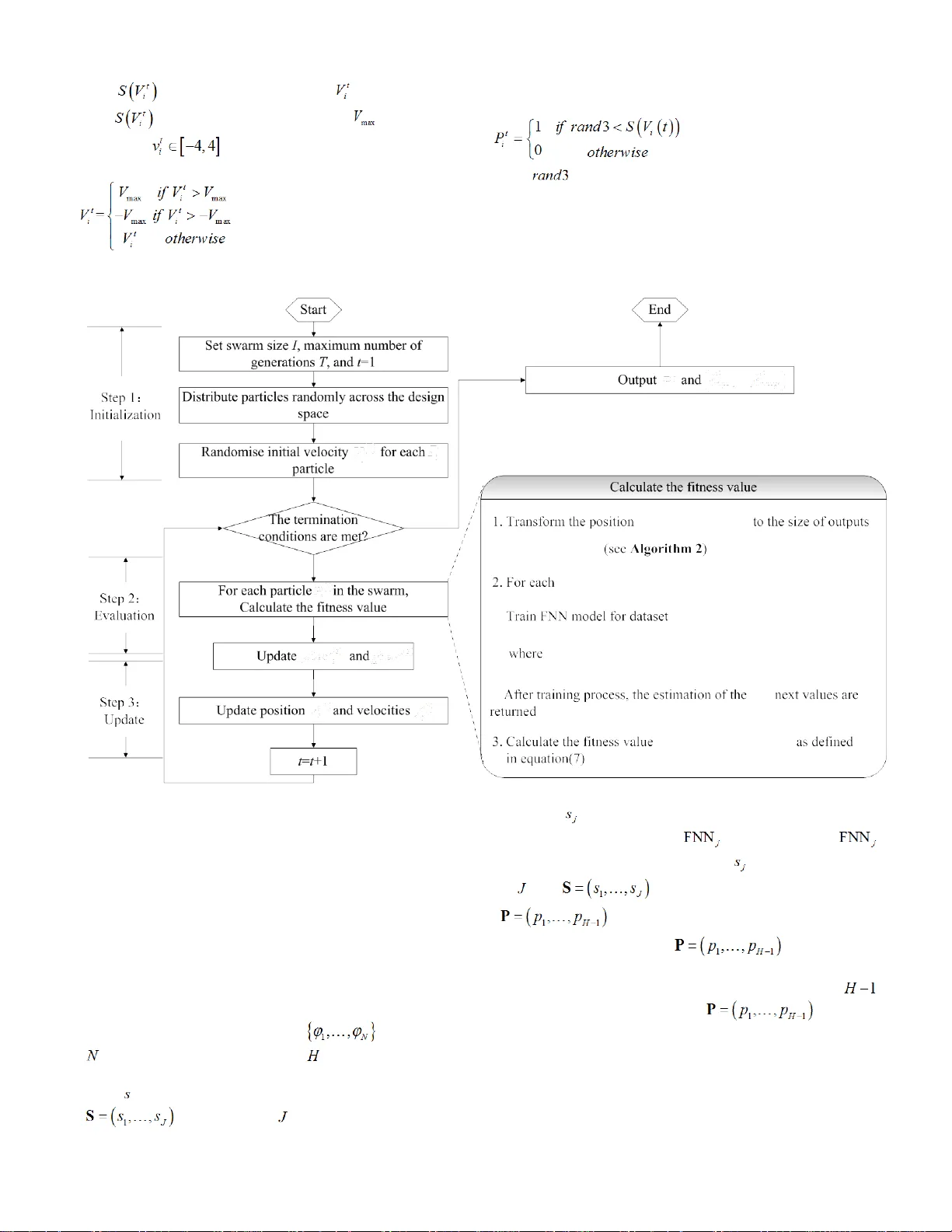
This is a preprint c opy that has be en accepted for public ation in IEEE T ransactions on C ybernetic s . Please c it e this article as: Y ukun Bao, T ao Xiong, Zhongyi Hu, “ PSO - MISMO Modeling Strategy for Multi - Step - Ahead T ime Series Predicti on”. IEEE T ransactions on Cyberneti cs . 2013 , accep ted . doi:10.1 1 09/TCYB. 2013. 2265084 . Copyright C laim: It should be note d that the copyright is rese rved by IEEE . T his preprint copy is onl y for personal use . Copyright © 2013 IEEE . All rights reserved. > REPLACE THIS LINE WITH YOUR PAPER IDENTIF ICATION NUMBER (DOUBLE - CLICK HERE TO EDI T) < 1 Abstract —M ulti - ste p - ahead time series prediction is on e of the most challenging research topic s in the field of time seri es modeling an d predicti on, and is conti nually under research. Recently, the m ultiple - input sever al m ultiple - ou tput s (MISMO) modeling strategy has been prop osed as a promising alternativ e for multi - step - ahead time series prediction, exhibiting advantages compared with the tw o currently dominating strategies , the itera ted and the direct strat egies. B uilt on th e establis hed MISMO strategy, this study proposes a p article s warm optimization ( PSO) - based MISMO mod eling strat egy, whi ch is capa ble of determi ning the number of sub -models in a self - adaptive mode, with varying prediction horizons. Rather than deriving crisp divides w ith equal - si ze s pr edicti on horizons fr om the establ ished MISMO, the proposed PSO - MISMO strategy, implemented with neural net works, emp loys a h euristic t o creat e flexible divides with varying size s of predicti on horizons and to generate correspondi ng sub - models, providing con siderable flexibility in model construct ion , whic h has been validated w ith si mulated and real datasets . Index Terms — Multi - step - ahead time series prediction , multiple - output models, particle swarm optimiz ation, genetic algorithm. I. I NTRODUCTION D espite intensive research efforts in time series mode ling and pre diction, most m odels c ontinue to be limited to one - step - ahead predict ion rat her tha n mult i - step - ahead prediction , primarily because of the challeng es ar ising from increased uncertainty fro m lo nger pred iction hor izons. The most c ommon m odeling s trategies for multi - step - ahead time series prediction re ly either on iterated or direct strategies [ 1-3]. An i t erated strategy first constructs a one - step - ahead p redict ion model , and the n uses the predi cted va lues as known da ta to Manuscript received Septe mber 12 , 2012 . This work was sup ported in part by the Natural Science Fou ndation of China under Grant No. 70771042, the Fundamental Research Fun ds for the Cen tral Universities (2012QN2 08 -HUST) , the MOE (Ministry of Edu cation in China) Project of Humanities and S ocial Science (Project No. 13YJA630002), and a gra nt from the Modern Inform ation Management Research Center at Hu azhong University of Science an d Technology. Yukun Bao (corr esponding auth or) , is with school of management, Huazhong University of Science and Technolo gy , Wuhan , P.R.Chi na (Tel: 86 - 27 - 87558579 ; fax: 86 - 27 - 875 56437 ; e -mail: yukunbao @ hust.edu.cn ). Tao Xiong, is with schoo l of management, Huazhong University of Science and Technology , Wuhan , P.R.China (e -mail: taoxiong @ hust.edu.cn ). Zhongyi Hu, i s with school of manageme nt, Huaz hong University of Science and Technolo gy , Wuhan , P.R.China (e -mail: huzhyi21 @ hust.edu.cn ). predict the ne xt ones . I n the direct strategy, a set of H predict ion mode ls are s olved t o predict values H step s ah ead. The acc umulati on of err ors in the iterated case deteriorates the accuracy of the prediction, and the direct strategy requires a sharply increa sed com putat ional e xpense, especially in the case of a lo nger pre dicti on horiz on. Base d upon t hese two mainstream modeling strategies, there has been a revival of interest in developing novel multi - step - ahead prediction strategies such as the DirRec strategy [4] , the m ultiple -i nput m ultiple -o utput (MIMO) strategy [5] an d m ultiple -i nput s everal m ultiple -o utput s ( MISMO ) strategy [ 6 , 7] (DIRMO in [8] ). A review an d com parative s tudy on strate gies fo r mul ti - step - ahead time series has indicated that the m ultiple -o utput strategies , including MIMO and MISMO (DIRMO) , a re the be st perf orming a pproach es, whic h has be en validated with NN5 f orecasting competition d ata [8]. This study focuses on a MISMO strategy , improv ing it in terms of modeling flexibility and more accurate prediction. MISMO is achi eved by transform ing the original H - step - ahead pr edicti on task i nto n Hs = subtas ks, yiel ding n sub- models w ith a f ixed number of multiple outputs , s , fo r each, where 1 sH ≤≤ . T he value of s is chosen through cross - validation , anal yz ing the perform anc e of the MI SMO model for different values o f s on the l earning set, a nd then us ing the best value to estimate the outputs [6 , 7] . In the sp ecial case where sH = , MI SMO can be r egar ded a s MIMO , and when 1 s = , MISMO is the same as a direct strategy. The superior ou t - of - sample performance of the MISMO strategy presented in [7] depend s on the trade - off between heterogeneity and com putationa l com plexit y. T he MISMO strategy exploits the heterogeneity across subtasks efficien tly, with less comput ational comple xity than the direct p rediction technique. An important feature of the MISMO strategy is that the origin al predict ion mo deling t ask is di vided i nto seve ral su btasks wi th an equal num ber of outp uts (pre dicti on horiz ons). Handling indivisibility in the problem is an explicit difficulty with the method. In addit ion, an under lying prob lem arises from the crisp di vides on t he pre diction h orizons with eq ual size s that induce a latent separation of dependenc ies am ong the s teps in the differe nt sub models. This problem may prevent the MISMO st rategy from c onsideri ng com plex depe ndenc ies between pr edict ion steps within di ffere nt sub mode ls and consequently reduce the prediction accuracy . Thus a st rategy with more flexibility and a mechanism to self -a daptively determine the prediction horizon di vides while modeling is appealing . This stud y proposes an improved P SO - MISMO PSO -MISMO Modeling Strategy for Multi-Step-Ahead T ime Series Prediction Yukun Bao , Member, IEEE, Tao X iong , Zhongyi Hu > REPLACE THIS LINE WITH YOUR PAPER IDENTIF ICATION NUMBER (DOUBLE - CLICK HERE TO EDI T) < 2 model ing strat egy for multi - step - ahead prediction that incorporates a heuristic based on particle swarm optimization (PSO) int o the MI SMO model ing pr ocess t o self - adaptively determ ine the num ber of sub - m odels with va rying pre dict ion horizons. For the p urpose of justi ficati on, this st udy com par es the rank of the p ropose d model ing stra tegy with the four well - established strategies ( i.e. , i terated, direct, MIMO and MISMO) wit h neural net works (NNs ). In addition, as a straight forwar d alter native, binary genet ic al gorithm - based MISMO modeling strategy (GA - MISMO) is selected as counterpar t against the propos ed PSO - MISMO and compared as well . Bo th simulated (i.e., Logistic and Mackey - Glass time series) and real (i.e., NN3 competition data) datasets are used for the compar isons. The paper is structured as follows. Section II provides a brie f rev iew of the multiple - output m odeli ng strategies , includi ng MIMO and MISMO , with li mited details. Section III describes the basic concept s of FNN for m ulti - step - ahead prediction and the im plementa tion of the FNN - base d predi ction m odel i n the current study. The co ncept o f the binary PSO is explained in Section IV . In Secti on V , detail s of the p ropose d PSO - MISMO strategy are presented . Section VI details the experimental setting on data, accuracy measure, genetic algorithm as al ternati ve, and e xperim enta l proced ure. E xperimental results are discussed in Section VII , and conc luding remarks are provide d in Se ction VI II . II. MIMO AND MISMO STRATE GIES Multi - step - ahead pre dictio n can be descri bed as an es tim ation of , ( 1, 2 , , ) Nh hH ϕ + =  , wh ere H is an i nteger greater than one, give n the curre nt and previo us obse rvati on , ( 1, 2 , , ) t tN ϕ =  . In this s ection , two com peting m odeli ng strategie s, MIMO a nd MISMO, with m ultiple - input multiple - output st ructure s for multi - step - ahead prediction are described , to enable underst anding of the pr opose d PSO - MISMO strategy in Section V. A. MIMO Strategy MIMO was first pr oposed in [5] and characterized as a multiple - input multiple - output approa ch, whe re the predi cted value i s not a scala r quant ity b ut a vect or of future values 12 ( , ,, ) N N NH ϕϕ ϕ ++ +  of the time series , ( 1, 2 , , ) t tN ϕ =  . Compared with the direct strategy, which estimates , ( 1, 2 , , ) Nh hH ϕ + =  using H model s, MIMO e mploys only one multiple - output m odel, p reservi ng the tempora l stoc hasti c dependenc y hi dden in t he pre dic ted time series. The MIM O modelin g strat egy l earns one multi ple - output forecasting model as follows: ( ) 11 ,, , () , ε i iH i id f ϕ ϕ ϕϕ + + −+ = +  (1) where d is the maximum embedd ing order and ε is a vector noise term of zero mean and nondiagonal c ovariance. After the learning proces s, the estimation s of t he H next values are returned according t o the f ollowi ng equat ion: ( ) 11 ˆ ( ,, ) ˆˆ ,, i iH i id f ϕ ϕ ϕϕ + + −+ =  (2) The limitation of MIMO lies in forcing all the prediction horizons to be predict ed wit h the sa me mode l struc ture (for instance, the same inputs ( ) 1 ,, i id ϕϕ −+  ), resulting in a reduction of the mode ling effort, but likely to bias th e returned model results . B. MISMO Str ategy A soluti on to th e shortcom ings of MIMO wa s propose d in [ 6 , 7] , where t he constra int of the fixed modeling structure is relaxed by tuning an integer paramet er s , which calibrates the dime nsionalit y of the o utputs on the basi s of a va lidati on criterion. For a given s , MISMO generate s n Hs = sub- models , which may have dif ferent i nput s from each other but a fixed size of o utputs at s , r esulting in slightly mor e modeling flexibility. The MISMO modeling strategy learns n multiple - output sub- models as follows: (3) where d is the m axim um em bedding or der an d ε is a zero - mean vector of size s . After the learning proces s, the estimation s of t he H next values are returned by the followi ng: ( ) { } ( 1) 1 1 ˆ ( ), ˆˆ ,, ,, 1, , . ik s s d k ik i i f kn ϕ ϕ ϕϕ + − + − −+ = ∈   (4) T he MISM O approa ch highl ights t he trade - off between th e property of pr eservi ng the s tocha stic de pendency am ong the predict ed valu es and the flexi bilit y of the m odeli ng proce dure [8] . However, the increased flexibility of the MISMO strategy requires an additional parameter s, wh ich give s rise to several issues in itself. An explicit issue is handling indivisibility when comput ing n Hs = , where all the parameters should be integer s . Further more, the num ber o f outp uts of every sub- model derived from MISMO i s fixe d a t s . This induc es a latent separation of depende ncies am ong the steps t hat may prevent the M ISMO st rategy from conside ring c ompl ex dependenc ies bet ween p redict ion st eps withi n diff erent sub- models and conse quentl y reduce the prediction accuracy. F urther s tudy has been solicited to determine the divid es of predict ion hor izons ada ptive ly whil e model ing rathe r tha n fixing th em at s . III. F EED - FORWARD NEURAL NETWO RKS Althou gh many types of neur al net works (NNs ) have be en propose d, the most pop ular o ne for t ime se ries pre dictio n is the feed - forward NNs (FN N s ). Because the focus of t his stu dy is the eval uation of the propose d model ing str ategy relati ve to the other com peti tors for m ulti - step - ahe ad pre diction, a simple three - layer FN N is impl emented t o mode l the selec ted strategies, capable of creating a common and reliable benchm ark. In additi on, the propos ed mode ling strate gy and t he four well - established strategies can all be implemented in t he FNN because o f the flexible struct ure of the F NN. Thus , the standard three - layer FNN with nodes i n adjacent layers fully connected i s used in this study. In this section, a short introduction to feed - forward neura l network s for mul ti - step - ahead predi ction is pr ovided, and then the ( ) { } ( 1) 1 1 ,, ( ) , 1, . , , , ε i k s i ks i i k d f kn ϕ ϕ ϕϕ + − + − −+ = +∈    > REPLACE THIS LINE WITH YOUR PAPER IDENTIF ICATION NUMBER (DOUBLE - CLICK HERE TO EDI T) < 3 implementation of the FNN - based predic tion m odel in t he current s tudy is de scribed . A. FNN for Multi - Step - Ahead Pre diction Fig. 1 s hows an e xam ple of a typica l three - layer FNN m odel with fou r input node s, fou r hidden n odes (one hidden la yer), an d two output neur ons used for multi - step -a head predict ion. The inp ut node s are the previ ous lag ged obse rvatio ns whil e the outputs pr ovide the fo recast for the future value s in a mul ti - step - ahead fashi on . Hidden nodes w ith appropriate nonlinear activation f unctions are us ed to p rocess the inform ation re ceived by the i nput node s. Bi as (or int ercept) terms are used both in the hidden and the output layers. To facilitate the understanding of t he FNN for multi - step - ahead time series prediction, the FNN with the MIMO modeling strategy will be u sed as an example in this section. Output Layer Hidden Layer Input Layer +1 t ϕ t ϕ -1 t ϕ -2 t ϕ -3 t ϕ +2 t ϕ Fig. 1. A three - layer feed - forward neural n etwork Given the training sample , the FNN mode l for H - step - ahead prediction can be written as follows : 00 11 , 1, , == y= + + = kn rr jh ij i j h ji w wx b b h H σ   …     ∑∑ (5) where x is the i nput ve ctor 1 () ,, i id ϕϕ −+  , y is the out put vector ( ) 1 ,, i iH ϕϕ ++  , w r , 0 w , b r , and 0 b are th e weigh ts and biases o f hidden and output la yers, n and H are the sizes of input and out put vect ors, k is the num ber of hidde n units, and ( ) σ ⋅ is a nonlinear activation function. Functionally, equation (5) can also be written as follows: ( ) ( ) 11 ,, ,, , = θ ε + i i H i id f ϕ ϕ ϕϕ + + −+  (6) w here ( ) f ⋅ represe nts the F NN m odel and θ is a vector that contains all the parameters in equation (5). The d etermination of parameter set θ is based on the local error between the measured ( ) 1 ,, i iH ϕϕ ++  and predicted values ( ) 1 ˆˆ ,, i iH ϕϕ ++  . In the c urre nt study , the m ean square e rror ( MSE) is use d as th e index of m ulti - step - ahead prediction perform ance to be minimize d , defined a s foll ows: ( ) 2 ++ =1 ˆ MSE= - H ih ih h H ϕϕ ∑ (7) B. Implementation of th e FNN - based Pre dicti on Mo del Following the procedure f rom [9] , t he design t asks f or the FNN - based predi ction m odel can be roughly divide d into four parts: data p reproce ssing, F NN desi gning, FNN implementation and validation. T he im plementa tion of the FNN - based model for m ulti - step - ahead predi ction is present ed step - by - step below:  Data preprocessing. Normalization is a standard requirement for time series modeling and prediction . Thu s, the data sets are first scaled by line a r transfere nce to map onto a range of [0, 1]. A fter the linea r transfere nce , deseasonaliz ation and detre nding a re performed when necessary . Deseasonalization is perfor med with the m ost recent X - 12 - ARIMA seasonal adjustment procedure. Detrendi ng i s p erformed by fitting a polynomial time trend to the data, and then s ubtrac ting t he estim ated tre nd from the series whe n tren ds a re detected by the Mann - Kendal l test .  FNN designin g. Selecting an appropriate architecture for the FNN is no rmally the first step wh en designing a n FNN - based pre diction sy stem . T he standard three - layer FNN with fully connected nodes in adjacent layers i s used in this study. T he number of i nput no des, hid d en nodes, output no des, a nd the ty pe of act ivatio n funct ions a re defined in the present study as follows . 1) Select ing the num ber of input nodes: The number o f input no des is determ ined by the i nput sel ection. The f ilter method, which s elects a set of inpu ts by optimizing a criteri on over differ ent com binati ons of i nputs by me ans of a search algorithm, i s empl oyed for i nput s elect ion in the current study. The f ilter method requires the setting of two elements: the criteri on , i.e., the statistic which estima tes the quality of the selected variables, and the search algorithm, which de scribe s the p olicy us ed to expl ore the input s pace. With respect to the cr iteri on , the partial mutual information [ 10 ] is used for the m odels using the iterated or direct strategies , and an extension of the Delta test [6] is used for the models with MIMO, MISMO , GA - MISMO, or PSO - MISMO strateg ies . W ith respect to the search algorithm , a forwa rd - backward selection method that offers the flexibility to reconsider input variables previou sly discarded and to discard input variables previously selected is used . The m axim um em bedding or der, d , is set to 15. 2) Select ing the num ber of hidde n nodes: T he numbe r of th e hidden node s cannot be determine d in advance . Thus empirical experimentations are need ed to d etermine this number [ 11 ] . Because of t he small sample size of many of the series, the experim entat ion is limited to five possible values of hidde n nodes , i.e., 2, 4, 6, 8 , or 10. The best number of hid den node s is de termi ned by us ing the origina l Akaike’s i nform ation crite rion (AIC ). 3) Selec ting th e num ber of o utput no des: T he num ber of output n odes is determ ined by the modeling strategy. M ost of the m odeling strate gies found in the literature can be classified into two categories, sing le - output st ructure and multiple - output st ructure . In the single - output s truct ure ( ) ( ) { } , = xy N dH ii id D = ∈ ℜ ×ℜ > REPLACE THIS LINE WITH YOUR PAPER IDENTIF ICATION NUMBER (DOUBLE - CLICK HERE TO EDI T) < 4 strategies , su ch as the it erated and direct strateg ies , multiple input s map t o a single output. The MIMO, MISMO, GA - MISMO, and PSO - MISMO strategies are all based on the multiple - output struc ture that ma ps m ultiple input s to multiple output s . Therefore , for t he iter ated a nd dire ct strategies, only one ou tput node is used for the FNN model. W hen em ploying the MIMO strat egy , t he n umbe r of outp ut nodes i s equal to the number of predi ction h orizon s . In th e MISMO strategy, the ori ginal H - step - ahead pr edicti on task s are separated in to n Hs = subtasks, resulting in n sub- models with fi xed m ultiple output s , s , for each, where 1 sH ≤≤ . Unlike the MI SMO strategy , which uses a fixed number of o utputs s for each sub - model, the GA - MIS MO and P SO - MISMO strat eg ies self - adaptively determines the number of sub - models with vary ing num ber of outputs , as described in Section V . 4) Selecting the type of activation fun ctions: A sigmoid transfer function is used at each hi dden no de and a l inear transfe r functio n is used at each out put node.  FNN im plement ation. T he L evenberg and M arquardt algorit hm (LM A) provi ded by t he MATLAB (Versi on 200 9 b) NN toolkit is used for th e training. N ode bias es are applied at the hidden a nd out put laye rs. For t he stop ping criteri on , the num ber of l earni ng epochs i s chos en as 1 000 , having no prior knowl edge of th e appropriate value. To determine the optimal parameters for the FNN, the co mmon practic e of five fold c ross - validation is used .  Validation: For each series of the simulated and real dataset , the la st 18 o bservat ions a re separ ated fo r ex - ante per formance assessment (out - of - sample), statistically indepen dent fr om the paramet er estim ati on process . The remainder of the data (in - sa mple ) i s used for param eter estimation an d the FNN mode ling. IV. B INARY PARTICLE SWAR M OPTIMIZ ATION Particle swarm optimizati o n (PSO) [ 12 ] is a population - based self - adaptive search algorithm that exploits a populat ion of indi viduals to probe pr omis ing regions of the search space. In the PSO, the population is referred to as a swarm that consists of a number of particles. Each particle repre sents a potential solution of the optimization task and has a position represented by a vector. Each particle moves to a new positio n accor ding t o both local i nform ation (t he par ticle memory ) and global inform ation (the knowled ge of all the particles). Thu s, t he PSO has the ability to converge to local and/or global o ptim al solut ions in a small num ber o f generat ions. In this sec tion, a brief i ntroduc tion t o a varia nt of the origi nal PSO, i.e., binary PSO, is present ed, to un dersta nd the mechanism of the pro pose d PSO - MISMO strategy applied in this s tudy . The P SO wa s initia lly desi gned to s olve conti nuous optimization problems. Since the in troduction of PSO, successful applications to several optimization problems [ 13 - 17 ] have dem onstr ated it s pote ntial. Howeve r, the m ajor o bstacl e of applying a PSO successfully is its continuous n ature. The first variant of the P SO algori thm f or solvi ng probl ems wit h binary - val ue sol ution el ement s (bina ry PSO) [ 18 ] was also develope d by t he creat or of the original PSO. The re are t wo key differe nces bet ween the bi nary PSO and the original PS O. The f irst difference is the representation o f the particle. In the binary PSO, every particle is characterize d by a binary solut ion representation (Note that th e representation is p rimarily related to a coding is sue in the pr oposed P SO - MISMO strat egy). The other difference is that the velocity of a particle in the binary PSO is a probability vector, where each pr obability element determines the likelihood of that binar y variable having the value o f one. Fig. 2 l ists t he ps eudoco de alg orithm for the basic binary PS O. Algorithm 1 Binary particle swar m optimization Initialize a po pulatio n of par ticle s with ran dom posit ions a nd velocities, throughout the input space. While not suffici ently goo d perform ance or maxim um num ber of iterations do for each particle { } 1, , i in I  do if ( ) ( ) ii f P f pbest < then ii pbest P = end if end ( ) ( ) { } ( ) { } min ** m i n , 1, , ii i pbest pbest f pbest f pbest i I = = ∈  if ( ) ( ) min f pbe st f gbest < then min gbest pbest = end if for each particle { } 1, , i in I  do Update velocity i V accordi ng to e quation (8). Update position i P accordi ng to e quation (11). end end while Fig. 2. Pseudocode fo r the binary PSO algo rithm The binary PSO up dates t he veloci ty acc ordin g to equation (8) as follo ws: ( ) ( ) 1 11 1 11 2 1 2 t t tt i i ii tt ii V w V c rand pbest P c rand gbest P − −− −− =⋅ +⋅ ⋅ − +⋅ ⋅ − (8) where 1 c and 2 c are the cognitive and interaction coefficients, 1 rand and 2 rand are rand om rea l num bers unifo rmly distributed b etween 0 and 1. w , the i ner t ia w eigh t, a user - specified parameter controls the momentum of the part icle. A larger ine rtia wei ght pushe s towa rds globa l explora tion wh ile a smaller inertia weight help s in fine - tuning the current search area. The following w eighting function is u sually utilized: () max min min Tt ww w w t − = −× + (9) where max w and min w are initial weight and final weight, respectively, T is the maximum number of allowable iterations and t is the current iteration. T he veloc ity is constra ined to the int erval [0 , 1] by us ing th e followi ng sigm oid tra nsform ation: ( ) ( ) 1 1 e xp t i t i SV V = −− ( 10 ) > REPLACE THIS LINE WITH YOUR PAPER IDENTIF ICATION NUMBER (DOUBLE - CLICK HERE TO EDI T) < 5 w here , is the prob ability that bit is equal to 1. T o avoid approac hing 0 or 1, a consta nt is often set at 4 such t hat , then the follo wing rela tionshi ps are applied: (1 1) Each particle, at each time step, changes its curr ent position according to equation ( 10 ), based on equation (1 2), as follows: (1 2) where is a ran dom rea l num ber unif orml y distri buted between 0 and 1. V. P ROPOSED PSO - MISMO MODELING STRAT EGY Fig. 3 . F lowchart of the propose d PSO -MISMO modeling strategy To address the limitation s of MISMO mentioned first in Section I and illustrated further in Section II .B , an i mprove d binary PSO - based MISM O is devel oped t hat self - adaptively determine s the number of sub - models with varying prediction horizons. T he proposed str ategy is abbreviated PSO - MISMO. Fig. 3 depi cts the flowcha rt of the propose d PSO - MISMO model ing strat egy. As shown in Fig. 3 , the detai led PSO - MISMO al gorithm consists of three major operat ions : initialization, evaluation , and update. Before describing d etails of these operat ions , coding issues will be addre ssed . The overall learni ng proce ss in Fig. 3 is elaborated step by step below.  Coding. C onsider a time series composed o f observat ions f or which the ne xt observat ions are to b e predicted . To avoi d the restriction associated with adopting a fixed in the original MISM O me thod, a fl exible ve ctor is used , where is the number of pred iction tasks, and represe nts the number of co nsecut ive out puts to be predicted at a tim e by the model (Note that model refers to the j th sub model with o utput s). The val ues of and are dete rmine d by the binary ve ctor that represents the se gment ation point ( see Algorithm 2 ). Each particle , represen ting a possible soluti on to the optim izati on problem , is det ermined by the binary PSO al gorit hm. The v alue s of compone nts of the bina ry vect or are ei ther 0 or 1 ; i f the va lue of a variabl e is 0, t hen the original task will not be divided by thi s segm entat ion point . I f the va lue of a variabl e is 1, t hen the prediction task will be divided by this segmentation point. Fig. 4 illustrates the solution representation. > REPLACE THIS LINE WITH YOUR PAPER IDENTIF ICATION NUMBER (DOUBLE - CLICK HERE TO EDI T) < 6 1 2 3 1 p 2 p 3 p   H 1 H − 1 H p − 2 H p − Prediction horizon Segmentation point Fig. 4 . Solution representatio n In the special case that { } 1, 1, 2 , , 1 i pi H = = −  , the strategy equals the direct strategy, and wh en { } 0, 1 , 2, , 1 i pi H = = −  , it equals the MIMO st rategy. For further illustration , assume a 10 - steps - ahead prediction task ( 10 = H ). Given t he binary vector ( ) 0, 0,1 , 0, 0, 0, 0, 1 , 0 P = , then ( ) 3, 5, 2 S = and 3 J = (see Algorithm 2 ). Thus, t he original task i s separated into three predic tion su btasks as follows: ( ) ( ) ( ) ( ) ( ) ( ) 12 3 1 1 1 45678 2 1 1 2 9 10 3 1 1 3 , , , , , , , , , , ,, , , ,, 1 ε ε ε i i i i i id ii iii i i i d i i i i id f f f ϕ ϕ ϕ ϕϕ ϕ ϕϕ ϕϕϕ ϕ ϕ ϕ ϕ ϕ ϕϕ ϕ + + + − −+ ++ +++ − − + + + − −+ = + = + = +    w here { } , 1, 2 , 3 ε i i = is a zero - mean vector of size 3, 5, 2. After t he lear ning pr ocess, the est imati on of t he ten next values i s retur ned by the thr ee ste ps as follows : ( ) ( ) ( ) ( ) ( ) ( ) 12 3 1 1 1 45678 2 1 1 9 10 3 1 1 ˆ ˆˆˆ , , , ,, ˆ ˆˆˆˆˆ , , , , , ,, ˆ ˆˆ , , ,, i i i i i id ii iii i i i d i i i i id f f f ϕ ϕ ϕ ϕϕ ϕ ϕϕ ϕϕϕ ϕ ϕ ϕ ϕ ϕ ϕϕ ϕ + + + − −+ ++ +++ − − + + + − −+ = = =    T he prediction horizons o f these pre diction sub - models (o r the num ber of outputs of the t hree FNN m odels) are 3, 5, an d 2, respecti vely. T his diff erence , or het erogenei ty, i s the hig hlight of the proposed strategy. For clarity, the flow of this example is illustrated in Fig. 5. 1 2 3 0 Prediction horizon Segmentation point 4 5 6 7 8 9 10 0 1 0 0 0 0 1 0 Original task Subtasks 1 2 3 Prediction horizon 4 5 6 Prediction horizon 7 8 9 10 Prediction horizon Subtask І Subtask Π Subtask Ш 10 = H 3 H = 5 H = 2 H = Fig. 5 . An example of s olution representation Algorithm 2. Computing t he value of ( ) 1 ,, S J ss =  Input : H , predict ion horiz on. Input : ( ) 11 ,, P H pp − =  , binary vector. Output: ( ) 1 ,, S J ss =  , j s represe nts the number of consecut ive o utputs t o be p redict ed at a tim e by the FNN j model 1 1 =1 H i i Jp − = + ∑ is the vector of size N =1 n for { } i n 1, , 1 iH −  do if 1 i p == then [ ] = SP n i =1 nn + end if end [ ] 1 =1 s SP [ ] = J s H SP N − for { } in 2, , 1 jJ −  do [ ] [ ] =1 j s SP j SP j −− end Return ( ) 1 ,, S J ss =  Fig. 6. Pseudoc ode for comput ing the value of ( ) 1 ,, S J ss =   Initialization. A ll the particles are ran doml y generat ed with 0 or 1 using a 50% probabi lity. A ll the velocity components are assigne d the ini tial va lue of 0. Concerning th e selection of parameters (i.e., inertia l weight w , coefficients 1 c and 2 c , swarm size I , and number of iteration s T ) in binary PSO, it is yet another challenging model selection task [ 19 ] . Fortunately, several empirical and theoretical studies have been perform ed about the parameters of PSO from which valuable information can be obtained [ 20 - 23 ] . In this study, the parameters are determined according t o the r ecomm endations in the se studi es and selected based on the predi ction pe rform ance and computational time in a trial - error fash ion . Tab le I su mmar ies the final parameters. TABLE I PARAMETER SELECTION OF B INARY PSO Parameters Values Swarm size I 20 Number of iterations T 100 Cognitive coefficient 1 c 2.0 Interaction coefficient 2 c 2.0 Initial weight max w 0.9 Final weight min w 0.4  Evalua tion. I n the current gener atio n t , for each particle ( ) t i p , the position ( ) 11 ,, P H pp − =  is trans forme d to 1 1 = H i i Np − = ∑ SP > REPLACE THIS LINE WITH YOUR PAPER IDENTIF ICATION NUMBER (DOUBLE - CLICK HERE TO EDI T) < 7 ( ) 1 ,, S J ss =  (see Algorithm 2 ). Then, e ach { } 1 ,, jJ ss s ∈  derived from the partic le ( ) t i p , is trained usi ng the training FNN i j model and the dataset ( ) ( ) { } , = xy j N s m j jj id D = ∈ ℜ ×ℜ , w here : { } 1 ,, -+ x, j nd n ϕϕ ⊂  ( ) 1 11 1 ,, - == ++ + y jj k k kk j n s ns ϕϕ   =  ∑∑    , 0 =0 s . After the training pr ocess, t he esti mati ons of th e next values of j s are returned. Once all H next val ues for parti cle ( ) ( ) ( ) { } 1 ,, tt t iI pp p ∈  are obtained, the fitness value of each particle ( ) t i p is calculated according to ( ) ( ) 2 ++ =1 ˆ MSE = - H t ii i Nh Nh h H ϕϕ ∑ , where + ˆ i Nh ϕ is the - h step - ahe ad forecast for particle ( ) t i p , + i Nh ϕ is the true value for particle ( ) t i p , and H is the prediction horizon .  Updat e. In the cur rent gene ration, o nce the fi tness val ues of all the particles in the swarm are calculated, the pbest of each particle, and the gbest of the swarm are obtained. Then, all the particles’ velocit ies and posi tion s are updated according to equatio ns (8) an d (1 2 ), respectively. If the termination conditions are met, then output gbest (that is, P* ) and th e corresponding - H step - ahead forecast { } ** +1 + ˆˆ ,, N NH ϕϕ  for particle P* ; otherwise , go back to the previous step. VI. E XPERIMENTA L SETTING A. Datase ts Description To evaluate the performances of the proposed PSO - MI SMO and the count erparts in terms of the forecast accuracy, two simulated time series, i.e., Logistic and Mackey - Glass time series, and a real world dataset, i.e., NN3 competition dataset, are used in this present study. Logistic and Mackey - Glass time series are recognized as benchm ark tim e series that ha ve been comm only us ed and reported by a number of studies related to time series modeling and forecasting [ 24 - 26 ]. The Logi stic m ap is a demogra phic m odel t hat was populari zed by May [27 ] as an example of a sim ple non - linear sy stem that exhibits complex, chaotic b ehavior. It is drawn from e quation ( 13 ). ( ) 11 41 ii i ϕϕ ϕ −− = − (13) The Mackey - Glass time series is approximated from the differential equation (14) (s ee [ 28 ] ). 10 d 0.2 0.1 d 1 ii i i i τ τ ϕϕ ϕ ϕ − − = − + (14) For each data - generating process (DGP), i.e., Logistic and Mackey - Glass process, we simulate twenty time series with different initialization and sample size, as was shown in Table II . The data for these time series are generated by the Chaotic Systems Toolb ox 1 TABLE II from the MATLAB s oftware. INITIALIZAT ION AND SA MPLE SIZE OF THE S IMULATED TIM E SERIES No. DGP Sample size Logistic ( 1 ϕ ) Mackey- Glass ( 1 ϕ , τ ) 1 0.100 1.000 15 485 2 0.125 1.200 15 496 3 0.150 1.400 15 523 4 0.175 1.600 15 548 5 0.200 1.800 15 674 6 0.225 2.000 15 692 7 0.2 60 1.000 16 726 8 0.275 1.200 16 758 9 0.300 1.400 16 779 10 0.325 1.600 16 791 11 0.350 1.800 16 821 12 0.375 2.000 16 843 13 0.400 1.000 17 869 14 0.425 1.200 17 889 15 0.450 1.400 17 912 16 0.475 1.600 17 926 17 0.5 10 1. 800 17 946 18 0.525 2.000 17 964 19 0.550 1.000 18 987 20 0.575 1.200 18 1002 The NN3 com petition was or ganize d in 20 07, ta rget ing comput ational - intelligence forecasting approaches. The compet ition d ataset of 111 monthl y tim e series dr awn from homoge neous po pulat ion of re al busi ness ti me seri es is u sed for evaluation 2 As such, three datasets of 20 Logistic time series, 20 Mackey - Glass time series, and 111 NN3 time series are used for evaluating the performanc es of the propos ed PSO - MISMO an d the co unter par ts in this s tudy. E ach series is split into an estimation s amp le and a hold - out sample. T he last 18 observat ions are saved for evaluating an d comparin g the out - of - sample forecast performances of the va rious mul ti - step - ahead predi ction strategies. All performance comparisons are based on these 18 . × 20 out - of - sampl e point s for Logis tic a nd Mackey - Glass datasets and 18 × 111 out - of - sam ple point s for NN3 datasets. B. Accuracy Measure For each pred i ction horizon h , three alternative forecast accuracy measures are co nsid ered : the m ean abs olute percent age er ror (M APE), the sy mmetri c me an absol ute percent age err or (SMAPE ), and t he m ean absolut e scale d error (MASE). The definiti on s of each are as follows: ++ =1 + ˆ - 1 MAPE = 100 mm M Nh Nh h m m Nh M ϕϕ ϕ ∗ ∑ (15) ++ =1 ++ ˆ - 1 SMAPE = 100 ˆ + mm M Nh Nh h mm m Nh Nh M ϕϕ ϕϕ ∗ ∑ (16) 1 Availabl e at http ://www.mat hwork s.com/matlab central/ fileexchan ge/159 7 2 Availabl e at http:/ /www.neural - for ecasting - competition.co m/NN3/datase ts.htm > REPLACE THIS LINE WITH YOUR PAPER IDENTIF ICATION NUMBER (DOUBLE - CLICK HERE TO EDI T) < 8 ++ =1 -1 =2 ˆ - 1 MAS E = 1 - -1 mm M Nh Nh h N mm m ii i M N ϕϕ ϕϕ ∑ ∑ (1 7) w here + ˆ m Nh ϕ is the - h step - ahead forecast for time series m , + m Nh ϕ is the true time series value for series m , H is the predict ion ho rizon (i n this c ase , =18 H ) and M is the num ber of time series in the datasets ( in this case , 20 M = for Logistic and Mackey - Glass datasets and = 111 M for NN3 d atasets ). For preproce ssed da ta , including normalization , deseasonalization and detre nding, we con vert the outputs from t he neural networks back to thei r origi nal sca les. P erformance prediction can then be compared directly. C. Genetic Algorithm as Alternative To furthe r asse ss the pe rform ance of the pro posed PSO - MISMO modeling strategy for multi - step - ahead prediction, we compare the experimental results of the PSO - MISMO with th ose prod uced by other di screte evoluti onary a lgorit hms, suc h as genet ic a lgorit hm (GA) (f or detailed introduction to GA , please refer to [ 29 - 31 ] ). This subsect ion brie fly pre sents t he im pleme ntation of GA - MISMO, a straightforward alt ern ative against PSO - MISMO . Fig. 7 depicts the f lowchart of the GA - MIS MO modeling strategy. As sho wn in Fig. 7, th e detailed GA - MISMO algorit hm consi sts of three m ajor parts : initializatio n, evaluation, and operatation . Before descr ibing details of these parts , coding issu es will be addressed . The overall learning process in Fig. 7 is elaborated step by ste p below.  Codi ng. The c hromosom e des ign in GA - M ISMO is the same with the particle design in PSO - MISMO, a s was prese nted in Section V . A c tually , the individual ( ) 11 ,, P H pp − =  may b e regarde d as chr omosom e in t erms of G A - MISMO, or as particle in terms of PSO - MISMO. The val ue s of 1 H − compone nts of the bina ry vec tor ( ) 11 ,, P H pp − =  are either 0 or 1 : if the value of a variable is 0, then the original task will not be divi ded by this s egme ntation point ; i f the value of a va riabl e is 1, t hen the prediction task w ill be divided by th is segme ntation poi nt. T he coding issue in GA - MISMO i s the same as PSO - MISMO and will not be presented in details her e to save space. TABLE III PARAMETER SELECTION OF GA Parameters Values Population size 20 Number of iterations 100 Crossover proba bility 0.90 Mutation probability 0.02  Initialization . A ll the chromosom es ar e randomly generated with 0 or 1 usin g a 50% probability. In se tting t he param eters of GA, it i s requi red to do extens ive sim ulations to fin d suit able values for various parameters. In this study, GA’s parameters are determined through p reliminary simulation and selected according to the recom menda tions in [ 32 - 34 ] in a trial - error fashion . Tab le III summarizes the final par ameter of GA.  Evaluation. The evaluation in GA - MISMO is the same as PSO - MISMO, as was presented in Sectio n V. Set population size I , maximum number of generations T , and t =1 Start Distribute chromosomes randomly across the design space The termination conditions are met? For each chromosome in the population, calculate the fitness value Apply GA operators: selection, crossover, and mutation t = t +1 End ( ) t i P Output and Yes No * P Step 1 ： Initialization Step 3 ： Operatation Step 2 ： Evaluation ( ) ** +1 + ˆˆ ,, N NH ϕϕ  Fig. 7 . F lowchart of th e GA- MISMO modeling s trategy  Operat ation . Designi ng the operator s for s electi on, cros sover, and mutation is a major issue in a GA implementation and is always done ad hoc. In each generation, after the fitne ss values of all the chromosomes in the sam e population are calculated, the selection operator that chooses c hromosomes from the current gener ation’s popul ation f or inclu sion in the n ext generation’s population is execute d. There are many ways for choosi ng parents [ 35 ] . I n this study, t he roulette m ethod is used for Logistic time series and top perce nt method is adopted for M ackey - Glass and NN3 time series through pr eliminary simulatio n in a trial - error fashi on. After selection of parents, the crossove r opera tor shoul d be appli ed to pr oduce t wo offspri ng by excha nging som e gene tic inf ormat ion betwe en the pa rents. Crossove r occurs duri ng evo lution a ccordi ng to t he cross over probability. The crossover probability i s how often a cross over will be perform ed. In t his study , the proba bilit y of cross over is set to 0.9, as sho wn in Ta ble III ; two - point o perator is us ed. This pr ocess of select ion and reproduc tion i s repeat ed unt il the number of offspri ng b ecomes equal to the num ber of eliminated chrom osomes; by addi ng the offspri ng to p opulati on, its size becomes equal to the initial size [ 34 ] . The muta tion is t he thi rd operato r, whic h is ap plied on the populat ion (par ents a nd thei r offsprin g) excl uding t he best c hromos ome. A sim ple m utation operator that selects a few percent of the genes of the population ra ndoml y and fli ps thei r values from zero to one and vice ver sa is used i n this st udy [ 36 ] . In this study, the probability of m utation is set to 0.02, as shown in Table III . Th e above process is repeated u ntil a termination conditions are reached . Once the termination conditions are met, the best chrom osome P* and the corres ponding - H step - ahead forecast > REPLACE THIS LINE WITH YOUR PAPER IDENTIF ICATION NUMBER (DOUBLE - CLICK HERE TO EDI T) < 9 { } ** +1 + ˆˆ ,, N NH ϕϕ  for c hrom osome P* are obtained ; otherwise , go back t o the previ ous step. D. Experi mental Procedure Start Split series into estimation sample and hold-out sample Perform Levenburg-Marquardt training algorithm and five-fold cross validation for model selection of FNN Conduct multi-step-ahead prediction using Calculate , , and for each prediction horizon and dataset Repeated 10 times? Calculate the mean of each accuracy measure End Yes No Conduct input selection Compare the quality of obtained results Input time series m =1 > mM Yes No = +1 mm th m Perform ANOVA and HSD test MAP E h SMAPE h MAS E h MISMO strategy Iterated strategy Direct strategy MIMO strategy PSO-MISMO strategy GA-MISMO strategy Fig. 8 . Experiment procedur e Fig. 8 shows the e xperim enta l proce dure using the simulated and real time series. Each series is first split into the estimation sampl e and the hold - out sam ple. T hen, the i nput se lecti on and model selection for each series are determin ed u sing the filt er method, th e Levenbe rg and M arquar dt al gorithm , and fi vefold cross - validation with iterated, direct, MIMO, MISMO, GA - MISMO, and PSO - MISMO s trategies. Finally the models are tested with the ho ld - out samples and the MAP E h , SMA PE h and MAS E h are computed for each prediction horizon h (in th is case = 1, 2 , h … ,18 ) ov er datasets (i.e., Logistic, Mackey - Glass , and NN3 datasets) . T he mode ling process for each series is repeated te n times. Upon the termi nation of this loo p, perf ormanc e of the exami ned model s with selected strategies a t each prediction horizon and dataset is judged i n term s of the mean, average d by ten, of the MAP E h , SMA PE h and MAS E h . A nalysis o f varianc e (ANOVA) tes t procedures are used to determi ne if the means of performance measures are significantly differe nt am ong the three m odels f or each prediction horizon and datasets . If so, Tuk ey’s honesty significant differenc e (HSD) tests [ 37 ] ar e then used to further identify the significantly diff erent prediction models in multiple pair - wise com parisons . VII. R ESULTS AND D ISCUSSION A. PSO - MISMO vs. the Others in Predictio n Accuracy The prediction performances of all six modelin g strategies exami ned in te rms of the three accuracy measures (MAPE, SMAPE, and MASE) and average ran k for thr ee dataset s ar e shown in Table IV . The colum ns labeled as ‘Average 1 - h ’ show the average accuracy measures over the prediction horizon 1 t o h . The last column sho ws the a verage ranki ng fo r each model over all p rediction horizons of the out - of - sample predict ion perf ormanc e. For e ach col umn of Table IV , the entry with the smallest value is set in boldface and m arked with an asterisk, and the entry with second smallest value is set in bold face type . T he results in Tab le IV lead to the following conclusions :  The ra nkings from best to worst are : PSO - MISMO and GA - MISMO are almost a tie , t hen MISMO , MIMO, direct, and iterated strateg ies , regardless of the accuracy m easures considere d. Thus our fi ndings are rob ust to t he choi ce of accuracy measures.  The modeling strategies based on th e multiple - output structure (i.e., PSO - MISMO, GA - MISMO, M ISMO, and MIMO strategies) outperform those based o n the si ngle - output structure (i.e., iterated and direct strategies) , which is in agreement with [7].  D espite the popularity of the iter ated strategy in mul ti - step - ahead predictio n literature, it is consistently the worst perfo rming strat egy for predic tion.  C om pari ng the iterated strategy with the direct strategy, the direct strategy is better regardless of the accuracy measures considered , which demonstrates that the accumulation of errors in the ca se of iterated strat egy drastically deteriorates the accuracy of the prediction.  The MIMO strategy consis tently achieves mor e accurate forec asts than either the iterated or the direct strateg ies for all prediction hor izons. It is conceivable that the reason for the superiority of the M IMO stra tegy i s that it pr eserves , am ong the predicted values, the stochastic dependency characterizing the ti me series.  The MISMO strategy seems to pro duce forecasts which are more accurate than tho se of the MIMO strategy (thoug h only marginally). It is conceivable that the reason for the superiority of the MISMO strategy is that it trades off th e property of pre servi ng the s tochast ic depe ndency between future value s with a greater flexibility of the predictor.  When compar ing the results of two heuristic - based modeling strategies (i. e., PSO - MIS MO and GA - MIS MO) with those o f MISMO strategy, the heuristic - based st rategies are generally better, which may ind icate that t he fixe d number of outputs of every sub - model derive d from the MISMO strategy tends to pre vent t he MIS MO st rategy from conside ring compl ex depende ncies betwee n predi ction steps wi thin differe nt sub m odels and conse quentl y reduces the prediction accuracy. > REPLACE THIS LINE WITH YOUR PAPER IDENTIF ICATION NUMBER (DOUBLE - CLICK HERE TO EDI T) < 10 TABLE IV PREDICTION ACCURACY MEASURES FOR HOLD- OU T SAMPLE Dataset Strategy Prediction horizon( h ) Average 1 - h Average Rank 1 2 3 6 12 18 1-3 1- 12 1- 18 Logistic MAPE ITER 47.89 39.94 39.41 43.28 35.21 51.41 42.41 43.18 46.18 5.888 DIR 47.93 37.18 36.27 41.71 36.14 49.22 40.46 42.95 44.87 5.000 MIMO 47.96 38.42 37.81 40.18 34.81 47.81 41.39 42.54 42.18 4.000 MISMO 47.96 37.64 35.54 41.21 34.15 45.12 40.38 41.54 41.84 3.111 GA- MISMO 47.88* 37.04 * 35.28 39.84 31.01* 43.01 40.06 * 39.24 39.14 1.555 PSO- MISMO 47.95 37.17 35.17 * 38.28* 32.73 42.18* 40.09 38.91* 38.51* 1.444* SMAPE ITER 31.10 33.42 36.74 39.74 45.12 39.21 33.75 39.13 40.14 5.888 DIR 30.97 32.02 37.18 36.18 45.85 37.44 33.39 38.67 38.79 5.055 MIMO 31.18 32.59 36.88 34.79 44.14 35.42 33.55 38.04 38.17 3.944 MISMO 30.87* 31.98 36.31 34.82 42.74 34.18 33.05 37.87 37.49 3.166 GA- MISMO 31.09 31.86 * 36.14 32.97 40.81* 32.95 33.03 35.41* 35.82 1.555 PSO- MISMO 31.11 32.03 35.74 * 33.58* 41.58 32.07* 32.96 * 36.13 35.18* 1.500* MASE ITER 0.706 0.521 0.911 0.914 1.184 1.054 0.713 0.941 1.124 5.944 DIR 0.705 0.501 0.894 0.881 0.914 0.867 0.700 0.887 0.914 4.944 MIMO 0.696 0.539 0.814 0.784 0.846 0.814 0.683 0.761 0.824 4.111 MISMO 0.691* 0.541 0.795 0.718 0.819 0.748 0.675 0.745 0.794 3.000 GA- MISMO 0.705 0.505 0.731* 0.624* 0.718* 0.642 0.647 0.687* 0.678* 1.444* PSO- MISMO 0.695 0.499* 0.742 0.648 0.743 0.618* 0.645 * 0.702 0.704 1.555 Mackey-Glass MAPE ITER 5.15 5.26 6.34 7.15 10.18 9.46 5.58 9.01 9.22 5.944 DIR 5.11* 4.93 5.87 6.92 8.55 8.49 5.30 7.83 8.13 5.055 MIMO 5.16 5.02 5.19 6.31 6.24 6.87 5.12 6.37 6.38 3.777 MISMO 5.13 4.88 5.23 5.87 5.97 6.05 5.08 5.89 5.64 3.222 GA- MISMO 5.16 4.87* 4.61 4.87* 4.28* 4.22* 4.88 4.78* 4.71* 1.444* PSO- MISMO 5.15 4.91 4.50 * 5.06 4.58 4.31 4.85* 4.96 4.87 1.555 SMAPE ITER 5.28 * 5.31 5.48 8.10 10.18 11.18 5.35 8.91 10.52 5.555 DIR 5.30 5.11 4.75 7.29 8.46 9.85 5.05 7.84 9.86 5. 000 MIMO 5.29 5.25 5.62 6.57 6.87 7.46 5.38 6.05 8.05 4.055 MISMO 5.31 5.05* 5.32 6.18 5.94 6.28 5.22 5.87 6.91 3.111 GA- MISMO 5.29 5.10 4.75 5.40 4.91 4.31* 5.04 5.16 5.19 1.611* PSO- MISMO 5.31 5.07 4.64 * 5.23* 4.72* 4.45 5.01* 5.12* 5.03* 1.777 MASE ITER 1.785 1.683 1.628 1.935 2.148 2.184 1.698 1.924 2.015 5.722 DIR 1.783 1.672 1.531 1.910 1.924 1.924 1.662 1.875 1.987 4.833 MIMO 1.769* 1.694 1.654 1.875 1.816 1.794 1.705 1.846 1.914 4.000 MISMO 1.775 1.681 1.615 1.849 1.748 1.649 1.690 1.789 1.841 3.055 GA- MISMO 1.781 1.663* 1. 522 1.746* 1.601 1.478 1.655* 1.710 1.647 1.666 PSO- MISMO 1.777 1.675 1.520* 1.759 1.588* 1.462* 1.657 1.703* 1.638* 1.611* NN3 MAPE ITER 14.93 13.69 17.05 19 .76 18.48 29.49 15.10 22.38 2 3.27 5.944 DIR 14.87* 12. 23 17.04 18. 87 17. 08 23. 84 14.71 17.29 18.74 5.000 MIMO 14.8 8 11. 68 17.09 18. 01 16. 07 21.54 14.55 16.41 17.57 4.055 MISMO 14.88 11.62 17.27 17.89 15.96 21.31 14.56 15.95 16.12 2.944 GA- MISMO 14.88 11.63 16.67* 17.20 15.04* 20.34 14.39* 15.68 16.03 1.611 PSO- MISMO 14.89 11.54* 16.84 17.1 5* 15.1 5 20.22 * 14.42 15.61* 15.9 1* 1.444* SMAPE ITER 15.1 6 13.31 14.97 20.57 17.84 20.68 14.48 19.97 21.59 5.944 DIR 15.1 0 1 1.84 14.34 18.37 15.67 19.97 13.76 17.75 19.84 5.000 MIMO 15.1 2 11.17 14.22 16.37 14.83 18.34 13.50 16.58 18.34 4.055 MISMO 15.10 10.97 13.37 15.97 14.56 18.16 13.14 16.13 17.10 2.944 GA- MISMO 15.09 * 10.88 13.21 * 15.86 13.43* 17.24* 13.06* 15.61* 16.47* 1.500* PSO- MISMO 15.1 1 10.68 * 13.46 15. 91* 13.61 17.38 13.08 15.72 16.51 1.555 MASE ITER 0.835 0.845 1.104 1.297 0.184 1.418 0.928 1.164 1.187 5.944 DIR 0.829* 0.859 1.197 1.168 0.108 1.387 0.962 0.109 1.046 5.055 MIMO 0.834 0.746 1.019 1.035 0.981 1.197 0.866 0.9 43 0.981 3.888 MISMO 0.834 0.741 0.996 1.007 0.975 1.184 0.857 0.923 0.934 3.055 GA- MISMO 0.835 0.731* 0.987 0.912 0.921* 1.083 0.856 0.910 0.917 1.555 PSO- MISMO 0.834 0.742 0.974* 0.9 07 * 0.92 6 1.0 61 * 0.850* 0.9 03 * 0.91 1* 1.500* Note: For each column of t able, the entry with the smallest value is set in boldf ace and marked with an asterisk, and the entry with secon d smallest value is set in boldface type. > REPLACE THIS LINE WITH YOUR PAPER IDENTIF ICATION NUMBER (DOUBLE - CLICK HERE TO EDI T) < 11 TABLE V MULTIPLE C OMPARISON RESULTS WITH RANK ED STRATEG IES FOR HO LD - OUT SA MPLE dataset Measure Prediction h orizon ( h ) Rank of strategies 1 2 3 4 5 6 Logistic MAP E h 4, 5, 8, 13, 16, 17 PSO- MISMO < GA- MISMO <* MISMO < MIMO <* DIR <* ITER 7, 9 - 11, 15 GA- MISMO < PSO- MISMO <* MISMO < MIMO <* DIR <* ITER 18 PSO- MISMO < GA- MISMO <* MISMO <* MIMO <* DIR <* ITER 12, 14 GA- MISMO < PSO- MISMO <* MISMO < MIMO < ITER < DIR 6 PSO- MISMO < GA- MISMO < MIMO < MI S MO < DIR <* ITER 2 GA- MISMO < PSO- MISMO < MISMO < DIR < MIMO <* ITER 3 PSO- MISMO < GA- MISMO < MISMO < DIR < MIMO <* ITER SMA PE h 6, 11, 14, 15, 18 PSO- MISMO < GA- MISMO <* MISMO < MIMO <* DIR <* ITER 5, 8, 13, 16 GA- MISMO < PSO- MISMO <* MISMO < MIMO <* DIR <* ITER 7 PSO- MISMO < GA- MISMO <* MISMO <* MIMO <* DIR <* ITER 10 PSO- MISMO < GA- MISMO < MIMO < MI S MO < DIR <* ITER 12, 17 GA- MISMO < PSO- MISMO <* MISMO <* MIMO < ITER < DIR 4, 9 PSO- MISMO < GA- MISMO < MISMO < DIR < MIMO <* ITER MAS E h 5, 10, 14, 15 PSO- MISMO < GA- MISMO <* MISMO < MIMO <* DIR <* ITER 7, 8, 11, 16, 17 GA- MISMO < PSO- MISMO <* MISMO < MIMO <* DIR <* ITER 9, 13 PSO- MISMO < GA- MISMO <* MISMO <* DIR < MIMO <* ITER 4, 12 GA- MISMO < PSO- MISMO < MISMO < MIMO <* DIR <* ITER 18 PSO- MISMO < GA- MISMO <* MISMO < MIMO < DIR < ITER 3 GA- MISMO < PSO- MISMO < MISMO < MIMO < DIR <* ITER 6 PSO- MISMO < GA- MISMO < MISMO <* MIMO <* DIR < ITER Mackey- glass MAP E h 5, 7, 10, 15 PSO- MISMO < GA- MISMO <* MISMO < MIMO <* DIR <* ITER 8, 9, 13, 16 GA- MISMO < PSO- MISMO <* MISMO < MIMO <* DIR <* ITER 4, 11, 14 PSO- MISMO < GA- MISMO <* MISMO <* MIMO <* DIR <* ITER 12, 17 GA- MISMO < PSO- MISMO < MISMO < MIMO <* ITER <* DIR 18 GA- MISMO < PSO- MISMO <* MIMO < MI S MO <* DIR <* ITER 6 GA- MISMO < PSO- MISMO <* MISMO < MIMO <* DIR < ITER 3 PSO- MISMO < GA- MISMO <* MIMO < MISMO <* DIR <* ITER SMA PE h 6, 9, 11, 13, 15 PSO- MISMO < GA- MISMO <* MISMO < MIMO <* DIR <* ITER 4, 7, 8, 14, 16, 17 GA- MISMO < PSO- MISMO <* MISMO < MIMO <* DIR <* ITER 12, 10 PSO- MISMO < GA- MISMO <* MISMO <* MIMO <* DIR <* ITER 18 GA- MISMO < PSO- MISMO <* MISMO <* MIMO <* ITER <* DIR 5 GA- MISMO < PSO- MISMO < MISMO <* MIMO <* ITER < DIR 3 PSO- MISMO < GA- MISMO < DIR < MISMO <* ITER <* MIMO MAS E h 7, 10, 11, 14, 16 PSO- MISMO < GA- MISMO <* MISMO < MIMO <* DIR <* ITER 5, 8, 13 GA- MISMO < PSO- MISMO <* MISMO < MIMO <* DIR <* ITER 18, 15 PSO- MISMO < GA- MISMO <* MISMO <* MIMO <* DIR < ITER 4, 17 GA- MISMO < PSO- MISMO < MISMO < MIMO <* ITER <* DIR 6, 9 GA- MISMO < PSO- MISMO <* MISMO < MIMO < DIR < ITER 3 PSO- MISMO < GA- MISMO <* DIR MISMO < ITER < MIMO 12 PSO- MISMO < GA- MISMO <* MISMO < MIMO <* ITER < DIR NN3 MAP E h 4, 6, 13,15,18 PSO- MISMO < GA- MISMO <* MISMO < MIMO <* DIR <* ITER 5, 8, 10 - 12 GA- MISMO < PSO- MISMO <* MISMO < MIMO <* DIR <* ITER 7, 16, 17 PSO- MISMO < GA- MISMO <* MISMO < MIMO <* DIR < ITER 9, 14 GA- MISMO < PSO- MISMO <* MISMO < MIMO <* DIR < ITER 2, PSO- MISMO < MISMO < GA- MISMO < MIMO <* DIR <* ITER SMA PE h 5, 7 - 9, 14,17 PSO- MISMO < GA- MISMO <* MISMO < MIMO <* DIR <* ITER 4, 10, 11, 12, 16 GA- MISMO < PSO- MISMO <* MISMO < MIMO <* DIR <* ITER 6 PSO- MISMO < GA- MISMO < MISMO < MIMO DIR <* ITER 13 PSO- MISMO < MISMO < GA- MISMO < MIMO <* DIR <* ITER 3, 15 GA- MISMO < PSO- MISMO < MISMO <* MIMO < ITER < DIR 18 GA- MISMO < PSO- MISMO < MISMO < MIMO <* DIR <* ITER 2 PSO- MISMO GA- MISMO < MISMO < MIMO <* DIR <* ITER MAS E h 5, 7, 8, 11 PSO- MISMO < GA- MISMO <* MISMO < MIMO <* DIR ITER 10, 13, 14, 16 GA- MISMO < PSO- MISMO <* MISMO < MIMO <* DIR <* ITER 9, 15, 18 PSO- MISMO < GA- MISMO <* MISMO < MIMO <* DIR < ITER 4, 12, 17 GA- MISMO < PSO- MISMO <* MISMO < MIMO < DIR <* ITER 2 GA- MISMO < MISMO < PSO- MISMO < MIMO <* DIR < ITER 6 PSO- MISMO < GA- MISMO < MISMO < MIMO <* DIR <* ITER 3 PSO- MISMO < GA- MISMO < MISMO < MIMO <* ITER < DIR Note: indicates the mean dif ference between the two adjacent strategies is sig nificant at the 0.05 lev el <* <* < <* * > REPLACE THIS LINE WITH YOUR PAPER IDENTIF ICATION NUMBER (DOUBLE - CLICK HERE TO EDI T) < 12  As far as the comparison between PSO - MISMO and GA - MISMO is concerned, they are alm ost a tie and the results are mi xing am ong the predict ion m easures exam ined . In ter ms of MAPE, PSO - MISMO wins in Logis tic dataset and NN3 dataset but loses in Mackey - Glass dataset. In terms of SMAP E, PSO - MISMO loses in Mackey - Glass dataset and NN3 dataset but wins in Logistic dataset . In terms of MASE, P SO - MISMO wins in Mackey - Glass dataset and NN3 dataset but loses in Logistic dataset . Followi ng the experi menta l proced ure pre sented in Fig. 8 , an ANOV A procedure is pe rform ed to determine if there exists a statistically sign ificant difference among the s ix modeling strategies in the ho ld - out sample for each of the performance measures and the prediction horizon. The results are n ot include d in deta il to save space. All ANOVA results are significant at the 0.05 level (with a few exc eptions) , suggesting that there are significant differences among the six m odeling strategies. To further identify the sign ificant difference between any two strategies, the Tukey’s HSD tes t is used to compare al l pair - wise differences simultaneou sly. Tukey’s HSD test is a post - hoc test, meaning that Tukey’s HSD test should not be performed unless the results of the ANOVA procedure are positive. Table V shows th e results of the multi ple com parison tests fo r three dataset s . F or each accuracy measure and prediction horizon, the stra tegies are ran k ordered f rom 1 (the best) to 6 (the worst). Several obser vations c an be ma de from Table V:  For each accuracy m easure and dataset , PSO - MISMO and GA - MISMO significant ly out perform s MISM O for t he overwhel ming m ajority of predic tion hori zon s.  Consi dering the two heuristic - based modeling strategies , we can see that, whatever the dataset used, whatever the accuracy measure conside red, an d wh atever the prediction horizon examined, the di fferenc e in prediction perform ance between PSO - MISMO and GA - MISMO is not significant at the 0.05 level .  As far a s the c ompari son MISMO vs. MIMO is concerned, t he difference in prediction performance is not significant at the 0.05 le vel , eve n with a few exceptions  Genera lly, t he stra tegies ba sed on t he singl e - output structure perform signifi cantly worse t han those based o n the multiple - output st ructure.  Conce rning t he cu rrent two leading strategies, the dir ect strategy significantly outperfo rms the iterated strategy for the majorit y of predi ction hori zon s.  The iterated strategy performs the poorest at 95% statistical confidence level in most cases, even with some exc eptions. B. PSO - MISMO vs. GA - MISMO in Convergence and Computat ional Time Up to no w, we ha ve compa red the propose d PSO - MISM O with othe r five competitors ( i. e. , iterated, direct, MIMO , MISMO , and G A - MIS MO ) in terms of prediction accuracy. In this su bsectio n, the c onverge nce and comput ationa l tim e of the two heuristic - b ased prediction stra tegies (i.e., PSO - MISMO and GA - MISMO) are furthe r exami ned. It shoul d be n oted t hat alth ough we have used a number of ti me series for each datasets, i.e., Logistic, Mackey - Glass, a nd NN3 datasets, general results do not change much within the time series for each datasets. Therefore, to save space, we report only the results for ran domly selected three time seri es from L ogi stic, Mackey - Glass, and NN3 datasets, respectively. They are the No.1 series from Logistic time series w ith 1 0.100 ϕ = and lengt h=485, the No. 18 serie s from Mackey - Glass time series with 1 2 ϕ = , 17 τ = , a nd length=964 , and the No.55 series from NN3 dat aset. In addi tion, in the following experiment, the swar m/population size is fixed to 20 for both PSO - MISMO and GA - MI SMO strategies, and generat ion nu mber i s set to 100, as desc ribed in Sec tion V. Each strategy is run ten tim es over each of these time series, i n an attempt to eliminate the influence of a lucky initial solution. All the numerical experiments are performed on a personal computer , Inter(R) Cor e(TM) 2 Duo CPU 2.50 GH z, 1.87 - G B mem ory, and MATLAB environment (Version R 200 9 b) . As was m entioned a bo ve, the learning process is repeated 10 times for both PSO - MISMO and GA - MISMO for ea ch time series. Thus, t ypica l conve rgence s of t he best and a verage fitness va lues as a fu nction o f genera tions for b oth PSO - MISMO and G A - MISMO on three afor ementioned time series are shown in Fig. 9( a) - (c), respectively. As it can be seen, in a typical PSO - MISMO optimization process the best fitness value dec rease s rapidl y and c onver ges at a bout 4 8 gene rations for No.1 Logistic time series , 65 generat ions for No.18 Mackey - Glass time series , and 59 gen era tions for N o. 55 tim e series in NN3 datasets; whereas f or GA - MISMO it tak es about 63 generat ions fo r No.1 Logistic time series , 77 generati ons fo r No.18 Mackey - Glass tim e series , and 6 8 generation s for No. 55 time series in N N3 datasets. To show how the evolut ion proc ess is going on for both PSO - MIS MO and GA - MISMO, the converge nce of the a verage fi tness value s are a lso sho wn in Fi g. 9. Looking at Fig. 9, it is cl ear that PSO - MIS MO seems to perform better than GA - MIS MO. Thus, for the pre sent pr oblem the p erformance of the PSO - MISMO is better than GA - MISMO from an ev olutiona ry point of view. 0 10 20 30 40 50 60 70 80 90 100 0.0612 0.2451 0.3185 0.4141 0.5386 0.6998 0.9098 Generation Fitnes s of PSO-M ISM O and GA-MISM O (MSE) (a) PSO-MISMO Best PSO-MISMO Average GA-MISM O Best GA-MISM O Average > REPLACE THIS LINE WITH YOUR PAPER IDENTIF ICATION NUMBER (DOUBLE - CLICK HERE TO EDI T) < 13 Fig. 9. Converge nce of best and av erage fitness for PSO - MIS MO and GA- MISMO strategies. (a) No .1 Logistic time series with 1 0.100 ϕ = and length=485. ( b) No.18 Mackey- Glass time series with 1 2 ϕ = , 17 τ = , and length=964.(c) No.55 ti me series in NN3 dataset. The second test performed is designed to measure the average computational time needed per time series from al l the datasets within these two strategies. The result is shown in Table VI , from which we can see th at the PSO - MISMO needs gener ally less time than GA - MISMO. TABLE VI COMPUTATION AL TIME F OR PSO - MISMO A ND GA - MISMO Dataset Strategy CPU time (M) Logistic dataset PSO- MISMO 24.514 GA- MISMO 38.421 Mackey- Glass dataset PSO- MISMO 30.824 GA- MISMO 41.725 NN3 dataset PSO- MISMO 11.854 GA- MISMO 19.627 General ly spea king, t hus, fr om t he above e xperim ents, w e can dra w the f ollowi ng three mai n conclusio ns. (1) Two heuristic - based modeling s trategies (i.e., PSO - MIS MO and GA - MISMO) are capable of obtaining high - quality mul ti - step - ahead time series forecasts related to the four well - establis hed strat egies . (2) The perf ormance of the PSO - MISMO is better than that of GA - MISMO f rom an evoluti onary poi nt of vie w. (3) P SO - MISMO showed to be faster than GA - MISMO i n term s of ave rage ru nning t ime . VIII. C ONCLUSIONS Multi - step - ahead tim e serie s predicti on has u sually proved t o be an i ntract able ta sk du e to t he gro wing am ount of uncerta inties a rising from various source s. For insta nce, a n accumulation of errors and lack of in form ation m ake mul ti - step - ahead pre diction more di fficu lt. Thus , mode ling strategies for multi - step - ahead prediction are major research topic s w ith significan t practical implication s . The contribut ion of t his study is a n extensi on to a well - establish ed MISMO model ing strat egy by i ncorp orating a heuri stic ba sed on binary particle swarm optimization into the MISM O mode ling proc ess to self - adaptive ly dete rmine t he num ber of sub - models with varying pred iction horizons, and conduct a large sc ale compara tive st udy with ne ural netw orks for validation . Q uantit ative a nd com prehensi ve asses sment s a re perf ormed with the simulated and real time series on the ba sis of the prediction accuracy , convergenc e, and c om putationa l time . Experimental results a nd com parisons de monst rate the superiority of the propos ed PSO - MISMO mode ling strategy for mul ti - step - ahead time series prediction. R EFERENCES [1] A. F. Atiya, S. M. El - Shoura, S . I. Shaheen , and M. S. E l - Sherif, "A comparison between ne u ral - network forecastin g techniques -case study: river flow forecasting ," Neural Networks, IEEE Transa ctions on, vol. 10, pp. 40 2 - 409, 1999. [2] G. Chevillon, "DIR ECT MULTI ‐ STEP EST IMATION AN D FORECASTIN G," J. Econ. Surveys , vol. 21, pp. 746 - 785, 2007. [3] A. Sorjamaa, J. Hao, N. Reyhani, Y. Ji, and A. Lendasse, "Methodology for long - term prediction of time series," Neurocomputin g, vol. 70, pp. 2861 - 2869, 2007. [4] A. Sorjamaa and A. Lendasse, "Time series predictio n using DirRec strategy," presented at the Euro pean Symposiu m on Artificial Neural Networ ks Bruges, 2006. [5] G. Bontempi, "Long term time serie s prediction with multi - input multi- output local learning," in Proceedings of the 2nd European Symposium on Time Series Predicti on (TSP), ESTSP08 , Helsink i , Finland, 2008, pp. 145 - 154. [6] S. Ben Taieb, G. Bontempi, A. Sorjamaa, and A. Lend asse, "Long - term prediction o f time series by combining direct and MIMO strategies," in Proceedings of t he 2009 IEEE International Joint Conference on Neural Networks , Atl anta, U.S.A., 2009, pp. 3054 - 3061. [7] S. Ben Taieb, A. Sorjamaa, an d G. Bontempi, "Multiple - output modeling for multi -step- ahead time series forecasting," Neurocomputin g, vol. 73, pp. 1950 - 1957, 2010. [8] S. Ben Taieb, G. Bontempi, A. F. Atiya, and A. Sor jamaa, "A review and comparison of strateg ies for multi - step ahead time series forecasting based on the NN5 forecastin g competition," Expert Syst. Appl., 2012. [9] H. S. Hippert, C. E. Pedreira, and R. C. Souza, "N eural networks for short - term load forecasting: A review and evaluation," Pow er Systems, IEEE Trans actions on, vol. 16, pp. 44 - 55, 2001. [10] A. Sharma, "Seasonal to in terannual rainfall probabilistic forecasts for improved water sup ply management: Part 1 — A s trategy for system predictor iden tification," J Hydrol, vol. 239, pp. 232 - 239, 2000. [11] G. P. Zhang and D. M. Kline, "Quarterly ti me - series forecasting with neural networks," Neural Networks, IEEE Tran sactions on, vo l. 18, pp. 1800 - 1814, 2007. [12] J. Kennedy and R. Eberhart, "Part icle swarm optimization," in Proceedings of the IEEE Internati onal Conference on Neural Networks , 1995, pp. 1942 - 1948 vol. 4. [13] C. F. Juang, "A hybrid o f genetic algorith m and particle swar m optimization for recurrent network design," Systems, Man, and Cybernetics, Part B: Cybernetics, IEEE Tra nsactions on, vol. 34, pp. 997 - 1006, 2004. 0 10 20 30 40 50 60 70 80 90 100 0.0026 0.0041 0.0066 0.0104 0.0166 0.0264 0.0420 0.0667 0.1062 0.1688 Generation Fitnes s of PSO-M ISM O and GA-MISM O (MSE) (b) PSO-MISMO Best PSO-MISMO Average GA-MISM O Best GA-MISM O Average 0 10 20 30 40 50 60 70 80 90 100 1051909 1199177 1367061 1558450 1776633 2025361 2308912 Generation Fitnes s of PSO-M ISM O and GA-MISM O (MSE) (c) PSO-MISMO Best PSO-MISMO Average GA-MISM O Best GA-MISM O Average > REPLACE THIS LINE WITH YOUR PAPER IDENTIF ICATION NUMBER (DOUBLE - CLICK HERE TO EDI T) < 14 [14] Y. P. Chen, W. C. Peng, and M. C. Jian, "Particle swarm optimization with reco mbination and dyna mic linkage disco very," Systems, Man, and Cybernetics, Part B: Cybern etics, IEEE Transactions on, vol. 37, pp. 1460 - 1470, 2007. [15] B. Liu, L. Wang, and Y. H. Jin, "An eff ective PSO - based memetic algorithm for flow shop scheduling, " Systems, Man, and Cybernetics, Part B: Cybernetics, IEEE Tra nsactions on, vol. 37, pp. 18 - 27, 2007. [16] R. Xu, J. Xu, and D. Wunsch, " A Comparison Study of Validity Indices on Swarm -Intelligence- Base d Clustering," Sys tems, Man, and Cybernetics, Part B : Cybernetics, IEEE Transactions o n, vol. 42, pp. 1243 - 1256, 2012. [17] T. Nguyen, S. Yang, an d C. Li, "A self - learning part icle swarm optimizer for global optim ization problem s," 2012. [18] J. Kennedy and R. C. Eb erhart, "A discrete binar y version of th e particle swarm algorithm," in Systems, Man, and Cyberne tics, 1997. Computational C ybernetics and Simulation., 1997 IEEE International C onference on , Orlando, FL, 1997, pp. 4104 - 4108 v ol. 5. [19] K. De Jong, "Parameter settin g in EAs: a 30 year perspective," in Parameter Setting in Evolutionary Alg orithms , ed: Springer, 2007, pp. 1 - 18. [20] I. C. Trelea, "The particle sw arm optimization algo rithm: convergence analysis and para meter selection," Inform Process Lett, vol. 85, pp. 317 - 32 5, 2003. [21] J. F. Kenne dy, J. Ken nedy, and R. C . Eberh art, Swarm i ntelligence : Morgan Kaufma nn Pub, 2001. [22] Y. Shi and R. C . Eberhart, "E mpirical study of particle swar m optimiza tion," in Evolutionary Comput ation, 1999. CEC 99. Proceedings of t he 1999 Congress on , 1999. [23] B. Liu, L. Wan g, and Y. - H. Jin , "An effective PSO - b ased memetic algorithm for flow shop scheduling, " Systems, Man, and Cybernetics, Part B: Cybernetics, IEEE Transactions on, vol. 37, pp. 18 - 27, 2007. [24] G. Rubio, H. Pomares, I . Rojas, and L. J. Her rera, "A heuristic method for para meter selection in LS - SV M: Application to ti me series prediction," Int J Foreca sting, vol. 27, pp. 725 - 739, 2011. [25] L. - C. Chan g, P. - A. Chen, and F. - J. Chang, "Reinf orced Two -Step- Ahead Weight Adju stment Technique for Onlin e Training of Recurrent Neural Networks ," Neural Networks and Learning Systems, IEEE Tr ansactions on, vol. 23, pp. 1269 - 1278, 2012. [26] Y. Liu and X. Yao, "Sim ultaneous tr aining of negativ ely correlated neural networks in an ens emble," Systems, Man, and Cyb ernetics, Part B: Cybernetics, I EEE Transactions o n, vol. 29, pp. 716 - 725, 1999. [27] R. M. May, "Simple mathematical models with very complicated dynamics," Nature, vol. 261, pp. 459 - 467, 1976. [28] M. C. Mackey and L. Glass, "Os cillation and chao s in physiological control systems," Science, vol. 197, pp. 287 - 289, 1977. [29] D. E. Goldberg, "Genetic algorith ms in search, optimization, an d machine learning," R eading, MA: Addison -Wesley, 1989. [30] K. M. Sim, "BLGAN: Bayesian lear ning and genetic algorith m for supporting negotiation with in complete infor mation," Systems, Man, and Cybernetics, Part B : Cybernetics, IEEE Transactions o n, vol. 39, pp. 198 - 211, 2009. [31] L. Davis, "Handboo k of genetic algorithms," New York: Va n Nostrand Rei nhold, 1991. [32] D. Golmohammadi, R. C. C reese, H. Valian, an d J. Kolassa, "Supplier selection based on a neural network model usin g genetic algorithm," Neural Networks, IEEE Tran sactions on, vol. 20, pp. 1504 - 1519, 2009. [33] D. E. Goldberg and K. Deb, "A co mparative analysis of s election schemes used in gen etic algorithms," Urbana, vol. 51, pp. 61801 - 2996, 1991. [34] M. V. Baghmisheh, K. Madan i, and A. Navarbaf, "A dis crete shuffled frog optimization algo rithm," Artif Intell R ev, vol. 36, pp. 267 - 284, 2011. [35] R. L. Haupt and S. E. Haupt, Practical genetic alg orithms : Wiley- Interscience, 2004 . [36] E. Elbeltagi , T. H egazy, and D. Grierson, "Compari son among five evolutionary- based opti mization algorithms," Adv Eng Inform, vol. 19, pp. 43 - 53, 2005. [37] F. Ramsay and D. Schaefer, The Sta tistical Sleuth : Duxbury, Boston, Mass, 1996. Yukun Ba o received h is B .S c., M .Sc., and Ph.D in m anagement s cience and e ngineeri ng from Huazh ong Unive rsity of Scienc e an d Technol ogy, P.R.Chi na, in 1996, 1999 an d 2002 respectively. Currently, h e is a n a ssociate p rofessor at the d epartment of m anagement s cience and i nformation systems, s chool of m anagem ent, Huaz hong Universi ty of Scienc e and T echnology , P.R .China. He has been the p rincipal investigator for two research p rojects funded by Natura l Scie nce Foun dation of China and ha s serve d as a referee of pape r review f or several I EEE journals and international journals and a PC member for several international academic conferences. His research interests are time series m odeli ng and foreca sting, busine ss inte llige nce and data m ining. Tao X io ng received his B .S c. and M .S c. in m anagement s cience and e ngineeri ng from Hua zhong Uni versit y of Sci ence and Tec hnolog y, P.R.C hina, i n 2008 a nd 2010 resp ectively. Currentl y, he is worki ng towar d the Ph.D. deg ree in m anagem ent s cience and e ngineeri ng, Huaz hong Un iversit y of Science and Tech nology, C hina. His research interests include mul ti - step - ahead time series forecasting, interval data analysis, computational intelligen ce . Zhongyi H u received B .S c. degree in i nform ation s ystem in 2009 from Harbin I nstitut e of Technol ogy at Weihai, P.R.Chin a. He received h is M .S c. d egree in m anagement s cience and e ngi neeri ng in 201 1 from Huazhong University of Science and Technol ogy, P. R.China. Currentl y, he i s worki ng tow ard the Ph.D . degree in m anagement s cience and e ngine ering, Huazhon g Universi ty of Scienc e and Techn ology, P. R. Chin a. His research interests include support vector machines, swarm intelligence, memetic algorithms, and time series for ecasting.