Frequentist and Bayesian measures of confidence via multiscale bootstrap for testing three regions

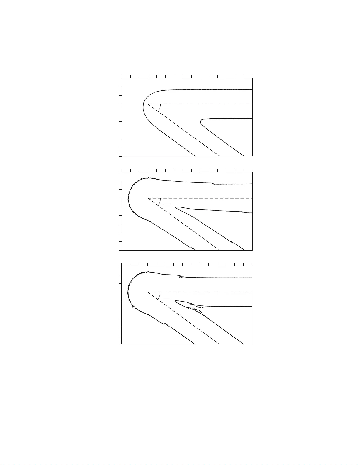
FREQUENTIST AND BA YESIAN MEASURES OF CONFIDENCE VIA MUL TISCALE BOOTSTRAP F OR TESTING THREE REGIONS HIDETOSHI SHIMODAIRA Abstract. A new computation method of frequen tist p -v alues and Bay esian posterior probabilities based on the b ootstrap probability is discussed for the multiv ar iate normal mo del with unkno wn exp ectation parameter vector. The n ull h ypothesis is represen ted as an arbitrary-shap ed region. W e introduce new parametric mo dels for the sc aling-law of bootstrap probability so that the multiscale bo otstrap method, which was designed for one-sided test, can also computes confidence measures of tw o-sided test, ex tending applicabili t y to a wider class of hypotheses. P aramet er estimation is improv ed by the tw o-ste p multiscale bo otstrap and also b y including higher-order terms. Model selection is i m portant not only as a motiv ating application of our m etho d, but also as an essential i ngredien t in the method. A compromise b et w een frequen tist and Ba y esian is attempted by showing that the Bay esian p osterior probability with an noninformative pr ior is inte rpreted as a frequent ist p -v alue of “zero-sided” test. 1. Introduction Let Y = ( Y 1 , . . . , Y m +1 ) b e a rando m vector of dimensio n m + 1 for so me in- teger m ≥ 1, and y = ( y 1 , . . . , y m +1 ) ∈ R m +1 be its observed v alue. Our ar- gument is based on the multiv ar iate normal mode l with unknown mean vector µ = ( µ 1 , . . . , µ m +1 ) ∈ R m +1 and cov ariance identit y I m +1 , (1) Y ∼ N m +1 ( µ, I m +1 ) , where the probability with resp e ct to (1) will be denoted as P ( ·| µ ). Let H 0 ⊂ R m +1 be an a r bitrary- s hap ed r egion. The sub ject o f this pap er is to c ompute measur es of confidence for testing the n ull hypothesis µ ∈ H 0 . Observing y , w e compute a frequentist p -v alue, denoted p ( H 0 | y ), a nd also a B ayesian p oster ior pro babilit y π ( H 0 | y ) with a no ninformative prior density π ( µ ) of µ . This is the pr oblem of r e gions disc ussed in liter ature; Efr on et al (19 96), Efr on and Tibshirani (1998), and Shimo daira (2002, 2004, 20 08). The confidence measures w ere calcu- lated by the bo otstr ap metho ds for complicated application problems such as the v ariable selection o f r egressio n analysis and ph ylogenetic tree selection of molecu- lar evolution. These mo del selection problems a re motiv ating applicatio ns for the issues discussed in this pap er, and the norma l mo del of (1) is a simplification of reality . Let X = { x 1 , . . . , x n } be a sample of size n in application pr oblems. W e assume there exists a transforma tion, dep ending on n , from X to y so that Y is Date : July 1, 2008. Key wor ds and phr ases. Approx imately un biased tests; Bo otstrap probability; Bi as corr ection; Hypothesis testing; Mo del selection; Probability match ing priors; Problem of regions; Scaling-la w . 1 2 HIDETOSHI SHIMOD AIRA approximately nor malized. W e assume only the existence of such a transformation, and do not have to consider its details. Since w e work o nly o n the transfor med v ari- able Y in this pap er for developing the theory , reader s ma y refer to the literature ab ov e for the exa mples of applications. Before the problem formulation is giv en in Section 2, our metho dology is illustrated in simple examples b elow in this sec tion. The s implest ex ample of H 0 would b e the half space of R m +1 , (2) H ′ 0 : µ m +1 ≤ 0 , where the notation H ′ 0 , instead of H 0 , is used to distinguis h this case fro m an- other example given in (3). Only µ m +1 is inv olved in this H ′ 0 , and one- dimensional normal mo del Y m +1 ∼ N ( µ m +1 , 1 ) is cons idered. T aking µ m +1 > 0 as an alter- native hypo thesis and denoting the cumulativ e distribution function o f the stan- dard normal as Φ( · ) with densit y φ ( · ), the unbiased f requentist p -v alue is given a s p ( H ′ 0 | y ) = Φ( − y m +1 ). A slig ht ly complex example o f H 0 is (3) H 0 : − d ≤ µ m +1 ≤ 0 for d > 0. The re jectio n regions are y m +1 > c and y m +1 < − d − c with a critical constant c , whic h is obtained as a solution of the equation (4) Φ( − c ) + Φ( − d − c ) = α for a sp ecified sig nificance level 0 < α < 1. The left hand s ide of (4) is the rejection probability P ( Y m +1 > c ∨ Y m +1 < − d − c | µ ) when µ is on the b oundary of H 0 , i.e., µ m +1 = 0 or µ m +1 = − d . The frequentist p -v alue is defined as the infimum of α such that H 0 can be r ejected. This b ecomes p ( H 0 | y ) = Φ( − y m +1 ) + Φ( − d − y m +1 ) for y m +1 ≥ − d/ 2 and p ( H 0 | y ) = Φ( y m +1 ) + Φ( d + y m +1 ) for y m +1 ≤ − d/ 2. C o nsidering the ca se, say , (5) d = 1 , y m +1 = − 0 . 1 , we obtain p ( H ′ 0 | y ) = 0 . 540 and p ( H 0 | y ) = 0 . 724. These tw o simple case s of H 0 and H ′ 0 exhibit what Efron and Tibshirani (199 8) called p ar adox of frequentist p -v alues. Our simple examples of (2) and (3) suffice for this purp os e, although they had actually us e d the spherical shell example explained later in Section 4. E fron and Tibshirani (19 98) indicated that a confidence mea sure should be monotonica lly inc r easing in the or der of set inclusion of the h yp othesis . Noting H 0 ⊂ H ′ 0 , therefore, it should be p ( H 0 | y ) ≤ p ( H ′ 0 | y ), but it is not. This kind of “para dox” cannot o ccur with Bayesian metho ds, and π ( H 0 | y ) ≤ π ( H ′ 0 | y ) ho lds alwa y s . Considering the flat prior π ( µ ) = cons t, say , the pos terior distribution of µ given y b ecomes (6) µ | y ∼ N m +1 ( y , I m +1 ) , and the p osterior probabilities for the case (5) a re π ( H ′ 0 | y ) = Φ( − y m +1 ) = 0 . 540 and π ( H 0 | y ) = Φ( − y m +1 ) − Φ( − d − y m +1 ) = 0 . 356 . The “ paradox” of frequentist p -v alues may b e nothing sur prise for a frequentist statistician, but a natural conse- quence of the fact that p ( H ′ 0 | y ) is for a one-s ided test a nd p ( H 0 | y ) is for a t wo-sided test; The p ow e r of testing is higher, i.e., p -v alues are s maller, for an appropriately formulated one-side d test than a t wo-sided test. In this pap er, we do not intend to argue the philosophical question of whether to b e frequen tis t or to be Bayesian, but discus s only computation of these t wo confidence measures. CONFIDENCE MEASURES VIA MUL TISCALE BOOTSTRAP 3 Computation of the confidence measur es is ma de by the b o otstra p r esampling of Efro n (1979). Let X ∗ = { x ∗ 1 , . . . , x ∗ n ′ } b e a b o otstra p sample of size n ′ obtained by res ampling with replacement fro m X . The idea of b o o tstrap probabilit y , which is intro duced fir st by F elsenstein (1985) to phylogenetic inference, is to generate X ∗ many times, say B , and count the frequenc y C that a hypothesis of int erest is suppor ted b y the bo o tstrap samples. The b o otstrap probability is computed as C /B . Recalling the transfo rmation to get y from X , we get Y ∗ by applying the same transformatio n to X ∗ . F or typical pr o blems, the v ar iance o f Y ∗ is appr oximately prop ortiona l to the factor σ 2 = n n ′ as mentioned in Shimo daira (2 008). Although we g e nerate X ∗ in practice, we only work on Y ∗ in this pap er. More sp ecifically , we formally consider the parametric bo o tstrap (7) Y ∗ | y ∼ N m +1 ( y , σ 2 I m +1 ) , which is ana logous to (1) but the scale σ is introduced for m ultiscale b o o ts tr ap. The b o otstrap probability is defined as (8) α σ 2 ( H 0 | y ) = P σ 2 ( Y ∗ ∈ H 0 | y ) , where P σ 2 ( ·| y ) denotes the pr obability with resp ect to (7 ). F or computing a crude confidence measure, w e set σ = 1, or n ′ = n in terms of X ∗ , so that the distr ibutio n (7) for Y ∗ is equiv a len t to the p os ter ior (6) for µ . This gives an in terpretation of the b o otstra p probability that α 1 ( H 0 | y ) = π ( H 0 | y ) for any H 0 under the flat prior. In the multiscale b o otstra p of Shimodair a (2002, 2004, 20 08), howev er , we may inten tionally alter the sca le from σ = 1, o r to change n ′ from n in terms of X ∗ for computing p ( H 0 | y ). Let σ 1 , . . . , σ M be M different v a lues of scale, which w e sp ecify in adv anc e . In o ur n umerical examples, M = 13 scales ar e equally spaced in log- scale b etw een σ 1 = 1 / 3 and σ 13 = 3 . F or each i = 1 , . . . , M , we genera te X ∗ with scale σ i for B i times, and observe the frequency C i . The observed b o otstrap probability is ˆ α σ 2 i = C i /B i . How can w e use the observed ˆ α σ 2 1 , . . . , ˆ α σ 2 M for computing p ( H 0 | y )? Let us assume tha t H 0 can be ex pressed as (3) but w e are una ble to observe the v alues of y m +1 and d . Nevertheless, by fitting the mo del α σ 2 ( H 0 | y ) = Φ( − y m +1 /σ ) − Φ( − ( d + y m +1 ) /σ ) to the observed ˆ α σ 2 1 , . . . , ˆ α σ 2 M , we may co mpute an es timate ˆ ϕ of the pa rameter vector ϕ = ( y m +1 , d ) with cons tr aints d > 0 and y m +1 > − d/ 2. The confidence measures are then computed a s p ( H 0 | y ) = Φ( − ˆ y m +1 ) + Φ( − ˆ d − ˆ y m +1 ) and π ( H 0 | y ) = Φ( − ˆ y m +1 ) − Φ( − ˆ d − ˆ y m +1 ). In case we are not sure whic h of (2) a nd (3) is the reality , w e may a lso fit α σ 2 ( H ′ 0 | y ) = Φ( − y m +1 /σ ) to the observed ˆ α σ 2 i ’s and co mpa re the AIC v alues (Ak aike, 1974) fo r mo del se le ction. In practice, we prepare collection of such mo dels describing the sca ling-law of b o otstra p pr obability , and choo se the mo del which minimizes the AIC v alue. 2. Formula tion of the pr oblem The exa mples in Section 1 were v ery simple b ecause the bo undary surfaces o f the regions are flat. In the following sections, we work o n generaliza tions of (2) and (3) b y allowing curved bo undary s urfaces. F or conv enie nc e , we denote y = ( u, v ) with u = ( y 1 , . . . , y m ) and v = y m +1 . Similarly , we denote µ = ( θ , µ m +1 ) with θ = ( µ 1 , . . . , µ m ) ∈ R m . As s hown in Fig. 1, we consider the region of the form 4 HIDETOSHI SHIMOD AIRA H 0 = { ( θ , µ m +1 ) | − d − h 2 ( θ ) ≤ µ m +1 ≤ − h 1 ( θ ) , θ ∈ R m } , where h 1 ( θ ) a nd h 2 ( θ ) are ar bitr ary functions of θ . This reg ion will reduce to (3) if h 1 ( θ ) = h 2 ( θ ) = 0 for all θ . The r egion may b e abbreviated as (9) H 0 : − d − h 2 ( θ ) ≤ µ m +1 ≤ − h 1 ( θ ) . Two other regions H 1 : µ m +1 ≥ − h 1 ( θ ) and H 2 : µ m +1 ≤ − d − h 2 ( θ ) as well a s tw o bo undary surfaces ∂ H 1 : µ m +1 = − h 1 ( θ ) a nd ∂ H 2 : µ m +1 = − d − h 2 ( θ ) a re a ls o shown in Fig. 1. W e de fine H ′ 0 = H 0 ∪ H 2 , o r equiv alently as (10) H ′ 0 : µ m +1 ≤ − h 1 ( θ ) . The b oundary s urfaces of the hypo theses ar e ∂ H 0 = ∂ H 1 ∪ ∂ H 2 for the region H 0 , and ∂ H ′ 0 = ∂ H 1 for the region H ′ 0 . W e do not hav e to specify the functional for ms of h 1 and h 2 for o ur theory , but assume that the mag nitude o f h 1 and h 2 is very small. T echnically s pea king, h 1 and h 2 are ne arly flat in the sense of Shimo daira (200 8). In tro ducing an artificial parameter λ , a function h is called near ly flat when sup θ ∈ R m | h ( θ ) | = O ( λ ) and L 1 - norms o f h and its F o urier transform a re b ounded. W e dev elop as ymptotic theo ry as λ → 0, which is analogous to n → ∞ with the r elation λ = 1 / √ n . The whole parameter spa ce is par titioned in to tw o regio ns as H ′ 0 ∪ H 1 = R m +1 or three regions as H 0 ∪ H 1 ∪ H 2 = R m +1 . Thes e partitions are treated as disjoint in this pap er by ignor ing measure- zero sets s uch a s H ′ 0 ∩ H 1 = ∂ H 1 . Bo otstrap metho ds fo r computing frequentist confidence measures are well developed in the literature as revie wed in Section 3. The main con tribution of our pap er is then given in Section 4 for the case of three r egions. In Section 5, this new computation metho d is used also for Bayesian measures of Efro n and Tibs hirani (199 8). Note that the fla t pr ior π ( µ ) = co nst in the previous section was in fact carefully chosen so that π ( H ′ 0 | y ) = p ( H ′ 0 | y ) for (2). This same π ( µ ) led to π ( H 0 | y ) 6 = p ( H 0 | y ) for (3). Our definition of H 0 given in (9) is a s imples t formulation, yet with a reasonable generality for applications, to observe such an interesting differ ence b e t w een the t wo confidence measures. Multiscale b o otstrap computation of the confidence measures for the three re- gions case is describ ed in Section 6. Simulation study and so me dis cussions are given in Section 7 a nd 8 , r esp ectively . Mathema tical pro ofs are mostly g iven in Appendix. 3. Frequentist measures o f confidence for testing two regions In this sectio n, we review the multiscale b o otstra p of Shimo daira (2008) for computing a frequentist p -v a lue of “one-sided” test of H ′ 0 . Let z = − Φ − 1 ( α ) b e the inv erse function of α = Φ( − z ). The b o otstrap z -v alue of H ′ 0 , defined as z σ 2 ( H ′ 0 | y ) = − Φ − 1 ( α σ 2 ( H ′ 0 | y )), is co nv enient to w ork with. By m ultiplying σ to it, σ z σ 2 ( H ′ 0 | y ) is calle d the no r malized b o ots tr ap z -v alue. Theorem 1 of Shimo daira (2008), as repro duced b elow, states that the z -v a lue of p ( H ′ 0 | y ) is obtained by extrap olating the normalized b o otstra p z -v alue to σ 2 = − 1, or equiv alen tly n ′ = − n in terms o f X ∗ . Theorem 1. L et H ′ 0 b e a r e gion of (10) with ne arly flat h 1 . Given H ′ 0 and y , c onsider the normalize d b o otst r ap z -value as a function of σ 2 ; We denote it by ψ ( σ 2 ) = − σ Φ − 1 ( α σ 2 ( H ′ 0 | y )) . L et us define a fr e quent ist p -value as (11) p ( H ′ 0 | y ) = Φ( − ψ ( − 1)) , CONFIDENCE MEASURES VIA MUL TISCALE BOOTSTRAP 5 H 1 y = (u,v) O v u H 0 H 2 h 1 h 2 d H 1 H 2 Figure 1. Region H 0 ⊂ R m +1 is the shaded area b et ween surfac e s ∂ H 1 and ∂ H 2 . and assume that the righ t hand side exists. Then for µ ∈ ∂ H ′ 0 and 0 < α < 1 , (12) P ( p ( H ′ 0 | Y ) < α | µ ) = α + O ( λ 3 ) , me aning t hat the c over age err or, i.e., t he differ enc e b et we en the r eje ction pr ob ability and α , vanishes asymptotic al ly as λ → 0 , and that the p -value, or the asso ciate d hyp othesis testing, is “similar on the b oundary” asymptotic al ly. Pro of. Here w e sho w only an outline of the pro of by allowing the coverage erro r of O ( λ 2 ), instead of O ( λ 3 ), in (12). This is a brief summa r y of the arg umen t given in Shimo daira (2008). First define the exp ectation op era tor E σ 2 for a nearly flat function h as ( E σ 2 h )( u ) := E σ 2 ( h ( U ∗ ) | u ) , where E σ 2 ( · ) on the right hand side deno tes the expecta tion with resp ect to (7), that is, for Y ∗ = ( U ∗ , V ∗ ) with U ∗ | u ∼ N m ( u, σ 2 I m ) , V ∗ | v ∼ N ( v, σ 2 ) . Using the expecta tio n op erato r, we next define t w o quantities z 1 = − v + E σ 2 h 1 ( u ) σ , ǫ 1 = − h 1 ( U ∗ ) − E σ 2 h 1 ( u ) σ , and work on the b o otstrap pro bability a s α σ 2 ( H ′ 0 | y ) = P σ 2 ( V ∗ ≤ − h 1 ( U ∗ ) | y ) = E σ 2 (Φ( z 1 + ǫ 1 ) | u ) = E σ 2 (Φ( z 1 ) + φ ( z 1 ) ǫ 1 | u ) + O ( λ 2 ) = Φ( z 1 ) + O ( λ 2 ) . (13) The third equation is obtained by the T aylor series around z 1 , and the last equatio n is obtained b y E σ 2 ( ǫ 1 | u ) = 0. Rearr a nging (13), we then get the scaling-law of the normalized b o otstra p z -v alue as (14) ψ ( σ 2 ) = v + E σ 2 h 1 ( u ) + O ( λ 2 ) . On the other hand, eq. (5.10) of Shimo daira (2008) shows, by utilizing F ourier transforms o f sur faces, that (12) holds with coverage e rror O ( λ 2 ) for a p -v alue 6 HIDETOSHI SHIMOD AIRA defined a s (15) p ( H ′ 0 | y ) = Φ( − v − E − 1 h 1 ( u )) + O ( λ 2 ) . The pro o f completes by combining (14) and (15).  A h yp othesis testing is to reject H ′ 0 when observing p ( H ′ 0 | y ) < α for a s pecified significance level, say , α = 0 . 05, and otherwise not to reject H ′ 0 . The left hand side of (12) is the rejection pro bability , which should be ≤ α for µ ∈ H ′ 0 and ≥ α fo r µ 6∈ H ′ 0 to claim the un biasedness of the test. On the other ha nd, the test is ca lled similar on the b oundary when the rejectio n probabilit y is equal to α for µ ∈ ∂ H ′ 0 . In this pa per , we implicitly assume that p ( H ′ 0 | y ) is decrea sing a s y mov es awa y from H ′ 0 . The rejection probability increases contin uously as µ mo ves aw ay from H ′ 0 . This ass umption is justified when λ is sufficiently small so that the b ehavior of p ( H ′ 0 | y ) is not v er y different from that for (2). Therefo r e, (12) implies that the p -v alue is a pproximately unbiased asy mptotically as λ → 0. W e can think o f a pro cedure for calculating p ( H ′ 0 | y ) base d on (11). In the pro cedure, the functional form of ψ ( σ 2 ) should b e estimated from the observed ˆ α σ 2 i ’s using pa rametric mo dels. Then an approximately unbiased p -v alue is computed by extrap olating ψ ( σ 2 ) to σ 2 = − 1. Our pro cedure w orks fine for the par ticula r H ′ 0 of (2 ), be c a use ψ ( σ 2 ) = y m +1 and p ( H ′ 0 | y ) = Φ( − y m +1 ) = Φ( − ψ ( − 1)). Our pro cedure works fine also for any H ′ 0 of (10) when the b oundar y sur face ∂ H ′ 0 is smo oth. The mo del is given as ψ ( σ 2 ) = β 0 + β 1 σ 2 + β 2 σ 4 + β 3 σ 6 + · · · using parameters ϕ = ( β 0 , β 1 , . . . ), a nd th us an approximately unbiased p -v alue can b e computed by p ( H ′ 0 | y ) = Φ( − ˆ β 0 + ˆ β 1 − ˆ β 2 + ˆ β 3 − · · · ). It may be int eresting to know that the parameters are in terpreted as geometric quantit ies; β 0 is the distance from y to the sur face ∂ H ′ 0 , β 1 is the mean curv atur e of the surface, and β j , j ≥ 2, is related to 2 j -th der iv atives of h 1 . How ever, the series expansio n ab ove do es not converge, i.e., ψ ( − 1) does no t exist, when ∂ H ′ 0 is nonsmo o th. F or exa mple, ψ ( σ 2 ) = β 0 + β 1 √ σ 2 serves as a go o d approximating model for co ne- shap ed H ′ 0 , fo r which ψ ( − 1) do es not take a v alue of R . This observ ation agree s with the fact that an unbiased test do es no t exist for cone-shap ed H ′ 0 as indica ted in the argument o f Lehma nn (19 52). Instea d o f (11), the mo dified pro cedure of Shimodair a (2008) calculates a p -v alue defined a s (16) p k ( H ′ 0 | y ) = Φ    − k − 1 X j =0 ( − 1 − σ 2 0 ) j j ! ∂ j ψ ( σ 2 ) ∂ ( σ 2 ) j    σ 2 0    for an in teger k > 0 and a rea l num ber σ 2 0 > 0. This is to extrap olate ψ ( σ 2 ) back to σ 2 = − 1 b y using the first k terms of the T a ylor series aro und σ 2 0 . The cov er age error in (12) should reduce as k increas es, but then the rejection reg io n violates the desired pro pe r ty called monotonicity in the sense of Lehmann (19 52) and Perlman and W u (1999, 2 003). F or taking the balance, we chose k = 3 and σ 2 0 = 1 for n umeric al examples in this paper . 4. Frequentist measures o f confidence f or testing three regions The fo llowing theo rem is our main result for computing a frequentist p -v alue of “tw o-s ided” test of H 0 . The proo f is giv en in Appendix A.1. Theorem 2. L et H 0 b e a r e gion of (9 ) with ne arly flat h 1 and h 2 . Given H 0 and y , c onsider t he appr oximately unbiase d p -value p ( H i | y ) by applying The or em 1 to H i CONFIDENCE MEASURES VIA MUL TISCALE BOOTSTRAP 7 for i = 1 , 2 . Assu m ing these two p -values exist, let us define a fr e quent ist p -value of H 0 as (17) p ( H 0 | y ) = 1 − | p ( H 1 | y ) − p ( H 2 | y ) | . F or example, (17) ho lds for the exact p -value of (3) defin e d in Se ction 1. Then for µ ∈ ∂ H 0 = ∂ H 1 ∪ ∂ H 2 and 0 < α < 1 , (18) P ( p ( H 0 | Y ) < α | µ ) = α + O ( λ 2 ) , me aning that p ( H 0 | y ) is appr oximately unbiase d asymptotic al ly as λ → 0 . F or illustrating the metho dolog y , le t us w ork on the spher ical shell example o f Efron and Tibshirani (1998), for which we can still compute the exact p -v alues to verify our methods . The region of interest is H 0 : a 2 ≤ k µ k ≤ a 1 as shown in Panel (a) of Fig. 2. W e consider the case, say , m + 1 = 4 , a 1 = 6 , a 2 = 5 , k y k = 5 . 9 , so that this region is analog ous to (5) e x cept for the curv ature. The exact p -v alue for H 1 : k µ k ≥ a 1 is easily calculated knowing that k Y k 2 is distributed as the chi- square distribution with degrees o f freedom m + 1 a nd noncentrality k µ k 2 . W riting this ra ndom v ariable as χ 2 m +1 ( k µ k 2 ), the exact p - v alue is p ( H 1 | y ) = P ( χ 2 m +1 ( a 2 1 ) ≤ k y k 2 ) = 0 . 36 2, that is, the proba bilit y of observing k Y k ≤ k y k fo r k µ k = a 1 . Similarly , the exa ct p -v a lue for H 2 : k µ k ≤ a 2 is p ( H 2 | y ) = P ( χ 2 m +1 ( a 2 2 ) ≥ k y k 2 ) = 0 . 267. In a similar wa y as for (3), the exa c t p -v alue for H 0 is computed n umerically as p ( H 0 | y ) = 0 . 907, a lthough the proc edure is a bit complicated a s explained below. W e fir st consider the cr itical cons tant s c 1 and c 2 for the rejection regions R 1 = { y | k y k < a 1 − c 1 } and R 2 = { y | k y k > a 2 + c 2 } . By equating the rejection proba bility to α for µ ∈ ∂ H 0 , that is , P ( χ 2 m +1 ( a 2 i ) < ( a 1 − c 1 ) 2 ) + P ( χ 2 m +1 ( a 2 i ) > ( a 2 + c 2 ) 2 ) = α for i = 1 , 2 , w e may get the s olution n umerically as c 1 = 1 . 331 and c 2 = 1 . 903 for α = 0 . 05, s ay . The p - v alue is defined a s the infimum o f α such that H 0 can b e rejected. T o chec k if Theorem 2 is ever usable, we firs t compute (17) using the exact v alues of p ( H 1 | y ) a nd p ( H 2 | y ). Then we get p ( H 0 | y ) = 1 − (0 . 36 2 − 0 . 26 7) = 0 . 905, which agr ees extremely well to the exa c t p ( H 0 | y ) = 0 . 907. The spherical shell is appr oximated b y (9) only lo c a lly in a neighborho od of y but not as a whole. Nevertheless, Theo r em 2 w or ked fine. W e next think o f the situation that bo otstrap probabilities of H 1 and H 2 are av aila ble but not their exact p -v alues. W e apply the pro cedur e of Section 3 sepa- rately to the tw o r egions for c alculating the a pproximately un bias e d p -v alue s . T o work on the pro cedure, here we consider a simple model ψ ( σ 2 ) = β 0 + β 1 σ 2 with parameters ϕ = ( β 0 , β 1 ) for (19) α σ 2 ( H ′ 0 | y ) = Φ( − ψ ( σ 2 ) /σ ) . Let ψ i ( σ 2 ) b e the normalize d bo o tstrap z -v alue of H i for i = 1 , 2. By assuming the s imple mo del for ψ i ( σ 2 ), we fit α σ 2 ( H i | y ) = Φ( − ψ i ( σ 2 ) /σ ) to the obser ved m ultiscale b o otstrap probabilities of H i for estima ting the parameters . T he actual estimation w a s done using the metho d described in Section 6.3, but w e w ould lik e to forget the details for the momen t. W e get ˆ β 0 = 0 . 1 01, ˆ β 1 = − 0 . 258 for H 1 , and similarly ˆ β 0 = 0 . 889 , ˆ β 1 = 0 . 286 for H 2 . β 0 ’s are in terpreted as the distances from y to the boundar y surfaces, and the estimates agree w ell to the exact v alues β 0 = 0 . 1 for H 1 and β 0 = 0 . 9 for H 2 . Then the approximately un bia sed p -v a lues 8 HIDETOSHI SHIMOD AIRA H 1 H 2 a 2 a 1 O y H 0 H 1 H 2 O H 0 y (a) (b) y Figure 2. (a) Spherical she ll region. (b) Cone-shap ed reg ion (Section 7). are computed by (11) as p ( H 1 | y ) = Φ( − 0 . 10 1 − 0 . 2 58) = 0 . 36 0 and p ( H 2 | y ) = Φ( − 0 . 889 +0 . 286 ) = 0 . 273 , a nd thus (17) gives p ( H 0 | y ) = 1 − (0 . 360 − 0 . 273 ) = 0 . 913, which ag ain ag r ees well to the exac t p ( H 0 | y ) = 0 . 907. W e finally think o f a more practical situation, wher e the b o ots tr ap pro babilities are not av ailable for H 1 and H 2 , but only for H 0 . This situatio n is plausible in applications wher e many regio ns are inv olved and we are not s ure which of them can b e trea ted as H 1 or H 2 in a neighbo rho o d of y ; See Efro n et al (1996) for a n illustration. W e consider a simple mo del ψ 1 ( σ 2 ) = β 0 + β 1 σ 2 , ψ 2 ( σ 2 ) = d − β 0 − β 1 σ 2 with pa r ameters ϕ = ( β 0 , β 1 , d ) for (20) α σ 2 ( H 0 | y ) = 1 − (Φ( − ψ 1 ( σ 2 ) /σ ) + Φ( − ψ 2 ( σ 2 ) /σ )) by as s uming tha t the tw o surfaces ar e curved in the same direction with the s ame magnitude of curv ature | β 1 | . F or estimating ϕ , (20) is fitted to the observed mul- tiscale bo o tstrap probabilities of H 0 with constraints β 0 > − d/ 2 and d > 0, and ˆ ϕ is obtained as ˆ β 0 = 0 . 089 , ˆ β 1 = − 0 . 19 9, ˆ d = 0 . 9 95. Then the a ppr oximately un biased p -v a lues are co mputed by (11) as p ( H 1 | y ) = Φ( − 0 . 08 9 − 0 . 19 9) = 0 . 38 7 and p ( H 2 | y ) = Φ( − 0 . 995 + 0 . 089 + 0 . 1 99) = 0 . 2 40 and thus (17) g ives p ( H 0 | y ) = 1 − (0 . 387 − 0 . 2 4 0) = 0 . 85 3. This is not v ery close to the exact p ( H 0 | y ) = 0 . 907, partly b eca use the model is to o simple. How ever, it is a g reat improv ement ov er α 1 ( H 0 | y ) = P ( a 2 1 ≤ χ 2 m +1 ( k y k 2 ) ≤ a 2 2 ) = 0 . 320. 5. Ba yesian measures of confidence Cho osing a g o o d prio r density is essential for Bay e s ian inference. W e conside r a v er sion of no ninformative prior for making the poster io r probabilit y acquire fre- quentist pro per ties. First note that the sum of b o otstra p probabilities o f disjoint partitions of the whole parameter space is alwa ys 1. F or the tw o reg ions ca se, α σ 2 ( H ′ 0 | y )+ α σ 2 ( H 1 | y ) = 1, a nd thus σ z σ 2 ( H ′ 0 | y ) + σz σ 2 ( H 1 | y ) = 0 . Therefor e p ( H ′ 0 | y ) + p ( H 1 | y ) = 1 for the approximately un biased p -v alues computed by (11), suggesting that we ma y think of a prior so that p ( H ′ 0 | y ) = π ( H ′ 0 | y ). T his was the idea of Efron and Tibs hirani (1998) to define a Bay e s ian meas ure of co nfidence of H 0 . Since each of H 1 and H 2 can b e treated as H ′ 0 by changing the co ordina tes, we may as sume a prior satisfying (21) π ( H i | y ) = p ( H i | y ) , i = 1 , 2 . CONFIDENCE MEASURES VIA MUL TISCALE BOOTSTRAP 9 It follows from P 2 i =0 π ( H i | y ) = 1 that (22) π ( H 0 | y ) = 1 − ( p ( H 1 | y ) + p ( H 2 | y )) . Prior s s atisfying (21 ) ar e called probability matching priors . The theo ry has b een developed in liter ature (Peers, 1965; Tibshirani, 1989; Datta a nd Mukerjee, 2004) for posterio r qua ntiles of a single par ameter of interest. The examples are the flat prior π ( µ ) = const for the flat boundary case in Section 1, and π ( µ ) ∝ k µ k − m for the spher ical shell case in Sec tio n 4. Our multiscale bo otstrap metho d pr ovides a new computation to π ( H 0 | y ). W e may simply compute (22) with the p ( H 1 | y ) and p ( H 2 | y ) used for computing p ( H 0 | y ) of (17 ). Although we implicitly as sumed the ma tc hing prio r, we do not have to know the functional for m of π ( µ ). F or the spherical s hell e xample, we may use the exact p ( H 1 | y ) and p ( H 2 | y ) to get p ( H 0 | y ) = 1 − (0 . 362 + 0 . 267) = 0 . 371, or more practically , use only bo otstrap pr o babilities of H 0 to get p ( H 0 | y ) = 1 − (0 . 38 7 + 0 . 240) = 0 . 373. 6. Estima ting p arametric models f or the scaling-la w o f bootstrap pr obabilities 6.1. One-step m ul tiscale b o o tstrap. W e first r ecall the estimation pro cedure of Shimodair a (2002, 20 0 8) before describing our new pr op osals for improving the estimation a c curacy in the following sections. Let f ( σ 2 | ϕ ) be a pa r ametric model of b o otstra p pr obability such as (19) for H ′ 0 or (20) for H 0 . As alr eady mentioned in Section 1, the mo del is fitted to the observed C i /B i , i = 1 , . . . , M . Since C i is distributed as binomial with probability f ( σ 2 i | ϕ ) and B i trials, the lo g-likelihoo d function is ℓ ( ϕ ) = P M i =1 { C i log f ( σ 2 i | ϕ ) + ( B i − C i ) lo g(1 − f ( σ 2 i | ϕ )) } . The maximum likelihoo d estimate ˆ ϕ is computed nu merically for each mo del. L e t dim ϕ denote the num ber of par ameters. Then AI C = − 2 ℓ ( ˆ ϕ ) + 2 dim ϕ may b e compared for se le cting a bes t mo del a mo ng several candidate mo dels. 6.2. Tw o -step multiscale b oots trap. Shimodair a (20 0 4) has dev is ed the mult istep- m ultiscale bo o tstrap as a genera lization o f the multiscale b o ots tr ap. The usua l m ultiscale b o ots tr ap is a sp ecial case called as the one-step m ultisc ale bo o ts tr ap. Our new pro po sal here is to utilize the tw o-step m ultiscale b o otstrap fo r improving the estimation accur a cy o f ϕ , although the tw o-step method was or iginally used for replacing the normal mo del of (1) with the exponential family of distributions. Recalling that X ∗ is obtained by resampling from X , we may resample again from X ∗ , instea d o f X , to get a b o otstrap sample o f size n ′′ , and deno te it as X ∗∗ = { x ∗∗ 1 , . . . , x ∗∗ n ′′ } . W e formally consider the parametric b o otstrap Y ∗∗ | y ∗ ∼ N m +1 ( y ∗ , ( τ 2 − σ 2 ) I m +1 ) , where τ is a new scale defined b y τ 2 − σ 2 = n/n ′′ . In Shimoda ira (2004), only the marginal distribution Y ∗∗ | y ∼ N m +1 ( y , τ 2 I m +1 ) is consider ed to detect the nonnormality . F o r the second step, P σ 2 ,τ 2 ( Y ∗∗ ∈ H 0 | y ) = α τ 2 ( H 0 | y ) should hav e the s ame functional form as P σ 2 ,τ 2 ( Y ∗ ∈ H 0 | y ) = α σ 2 ( H 0 | y ) for the norma l mo del. Here we also co nsider the join t distr ibution o f ( Y ∗ , Y ∗∗ ) g iven y . It is 2 m + 2- dimensional mult iv ariate no r mal with C ov ( Y ∗ , Y ∗∗ | y ) = σ 2 I m +1 . W e denote the 10 HIDETOSHI SHIMOD AIRA probability and the exp ectatio n by P σ 2 ,τ 2 ( ·| y ) and E σ 2 ,τ 2 ( ·| y ), resp ectively . Then, the joint b o otstrap probabilit y is defined as α σ 2 ,τ 2 ( H 0 | y ) = P σ 2 ,τ 2 ( Y ∗ ∈ H 0 ∧ Y ∗∗ ∈ H 0 | y ) . Let g ( σ 2 , τ 2 | ϕ ) b e a pa rametric mo del of α σ 2 ,τ 2 ( H ′ 0 | y ) o r α σ 2 ,τ 2 ( H 0 | y ). T o work on sp ecific forms of g ( σ 2 , τ 2 | ϕ ), we need some no tations. Let ( X ′ , X ′′ ) b e dis- tributed as biv aria te normal with mean (0 , 0), v ariance V ( X ′ ) = V ( X ′′ ) = 1, and cov a riance C ov ( X ′ , X ′′ ) = ρ . The distribution function is denoted as Φ ρ ( a 1 , b 1 ) = P ( X ′ ≤ a 1 ∧ X ′′ ≤ b 1 ), wher e the join t density is explicitly given as φ ρ ( a 1 , b 1 ) = (1 − ρ 2 ) − 1 / 2 φ ((1 − ρ 2 ) − 1 / 2 ( b 1 − ρa 1 )) φ ( a 1 ). W e also define Φ ρ ( a 1 , b 1 ; a 2 , b 2 ) = P ( a 2 ≤ X ′ ≤ a 1 ∧ b 2 ≤ X ′′ ≤ b 1 ) = Φ ρ ( a 1 , b 1 ) − Φ ρ ( a 2 , b 1 ) − Φ ρ ( a 1 , b 2 ) + Φ( a 2 , b 2 ). Then a generalizatio n of (14) is giv en a s follows. The pro of is in Appendix A.2. Lemma 1. F or sufficiently smal l λ , the joint b o otstr ap pr ob abilitie s for H ′ 0 and H 0 ar e expr esse d asymptotic al ly as α σ 2 ,τ 2 ( H ′ 0 | y ) = Φ ρ ( z 1 , w 1 ) + O ( λ 2 ) , (23) α σ 2 ,τ 2 ( H 0 | y ) = Φ ρ ( z 1 , w 1 ; z 2 , w 2 ) + O ( λ 2 ) , (24) wher e z 1 = − ( v + E σ 2 h 1 ( u )) /σ , w 1 = − ( v + E τ 2 h 1 ( u )) /τ , z 2 = − ( v + d + E σ 2 h 2 ( u )) /σ , w 2 = − ( v + d + E τ 2 h 2 ( u )) /τ , and ρ = σ /τ . Thu s g ( σ 2 , τ 2 | ϕ ) is sp ecified for H ′ 0 as (23) with z 1 = − ψ ( σ 2 ) /σ , w 1 = − ψ ( τ 2 ) /τ using the ψ function of (19). Similarly , g ( σ 2 , τ 2 | ϕ ) is sp ecified for H 0 as (24) with z 1 = ψ 1 ( σ 2 ) /σ , w 1 = ψ 1 ( τ 2 ) /τ , z 2 = − ψ 2 ( σ 2 ) /σ , w 2 = − ψ 2 ( τ 2 ) /τ using ψ 1 and ψ 2 functions o f (20). W e may sp ecify M sets of ( σ , τ ), denoted as ( σ 1 , τ 1 ) , . . . , ( σ M , τ M ). In o ur nu merical examples , σ 1 , . . . , σ 13 are sp ecified as mentioned in Section 1 and τ i ’s are specified so that τ 2 i − σ 2 i = 1 holds alwa ys, mea ning n ′′ = n . F or each i = 1 , . . . , M , we generate ( Y ∗ , Y ∗∗ ) with ( σ i , τ i ) ma ny times, say B i = 10 000, and obse r ve the freq uencies C i = #( Y ∗ ∈ H 0 ), D i = #( Y ∗∗ ∈ H 0 ), and E i = #( Y ∗ ∈ H 0 ∧ Y ∗∗ ∈ H 0 ). Note that only one Y ∗∗ is generated from each Y ∗ here, whereas thousands of Y ∗∗ ’s may b e generated from e a ch Y ∗ in the double b o otstrap metho d. The log-likelihoo d function b ecomes ℓ ( ϕ ) = P M i =1 { E i log g ( σ 2 i , τ 2 i | ϕ ) + ( C i − E i ) lo g( f ( σ 2 i | ϕ ) − g ( σ 2 i , τ 2 i | ϕ )) + ( D i − E i ) lo g( f ( τ 2 i | ϕ ) − g ( σ 2 i , τ 2 i | ϕ )) + ( B i − C i − D i + E i ) lo g(1 − f ( σ 2 i | ϕ ) − f ( τ 2 i | ϕ ) + g ( σ 2 i , τ 2 i | ϕ )) } . In fact, we hav e used this t wo-step m ultisc a le b o otstra p, instead o f the one- step metho d, in all the numerical examples. The one-s tep metho d had difficult y in distinguishing H 0 with very s mall d fr o m H 0 with mo der ate d but heavily curved ∂ H 1 . The tw o -step metho d avoids this ident ifiability issue b ecause a sma ll v alue o f E i indicates that d is small; It is automatically done, of cour se, by the numerical o ptimization of ℓ ( ϕ ). 6.3. Higher-order terms of b o otstrap probabili ties for tes ting t wo regions. The asympto tic errors of the scaling law of the bo otstra p proba bilities in (1 3) and (23) are of or der O ( λ 2 ). As sho wn in the following lemma, the e rrors can b e r educed to O ( λ 3 ) by introducing cor rection terms of O ( λ 2 ) fo r improving the parametric mo del g ( σ 2 , τ 2 | ϕ ) of H ′ 0 . The proo f is giv en in Appendix A.3. CONFIDENCE MEASURES VIA MUL TISCALE BOOTSTRAP 11 Lemma 2. F or sufficiently smal l λ , the b o otst ra p pr ob abilities for H ′ 0 ar e expr esse d asymptotic al ly as α σ 2 ( H ′ 0 | y ) = Φ( z 1 + ∆ z 1 ) + O ( λ 3 ) (25) α τ 2 ( H ′ 0 | y ) = Φ( w 1 + ∆ w 1 ) + O ( λ 3 ) (26) α σ 2 ,τ 2 ( H ′ 0 | y ) = Φ ρ +∆ ρ ( z 1 + ∆ z 1 , w 1 + ∆ w 1 ) + O ( λ 3 ) , (27) wher e z 1 , w 1 , and ρ ar e those define d in L emma 1, and the h igher or der c orr e ction terms ar e define d as ∆ z 1 = − 1 2 z 1 E σ 2 ,τ 2 ( ǫ 2 1 | u ) , ∆ w 1 = − 1 2 w 1 E σ 2 ,τ 2 ( δ 2 1 | u ) , and ∆ ρ = − 1 2  ρE σ 2 ,τ 2 ( ǫ 2 1 | u ) + ρE σ 2 ,τ 2 ( δ 2 1 | u ) − 2 E σ 2 ,τ 2 ( ǫ 1 δ 1 | u )  using (28) ǫ 1 = − h 1 ( U ∗ ) − E σ 2 h 1 ( u ) σ , δ 1 = − h 1 ( U ∗∗ ) − E τ 2 h 1 ( u ) τ . F or deriv ing a very simple mo del for ∆ ρ , we think o f a situa tio n h ( u ) = ( A/ √ m ) k u k + ( B /m ) k u k 2 and θ = 0, and co nsider asymptotics as m → ∞ . This formulation is only for convenience o f deriv atio n. The t wo v alues A a nd B will be sp ecified later by looking a t the functional fo rm of f ( σ 2 | ϕ ). A stra ightf orward, y et tedious, cal- culation (the details are not s hown) gives ψ ( σ 2 ) = const + Aσ + B σ 2 + O ( m − 1 ) and ∆ ρ = − 1 2 m  A 2 ρ (1 − ρ ) + 2 B 2 ρ ( τ 2 − σ 2 ) + 2 AB σ (1 − ρ 2 )  + O ( m − 3 / 2 ) . This correc tio n term was in fact alrea dy used for the simple mo del ψ ( σ 2 ) = β 0 + β 1 σ 2 of the s pherical shell example in Sectio n 4, where the parameter was actually ϕ = ( β 0 , β 1 , m ) instead of ϕ = ( β 0 , β 1 ). W e did not c ha nge the ψ ( σ 2 ) for adjusting ∆ z 1 and ∆ w 1 , meaning that z 1 + ∆ z 1 , instead of z 1 , was mo delled as − ψ ( σ 2 ) /σ . Comparing the co efficients o f ψ ( σ 2 ), we get A = 0 and B = β 1 , and th us ∆ ρ = − ( β 1 ) 2 ( σ /τ )( τ 2 − σ 2 ) /m . When (19) was fitted to H 1 , the e stimated parameter ˆ m = 2 . 8 3 was close to the true v alue m = 3. F or the numerical example mentioned above, we ha ve also fitted the s ame model but ∆ ρ = 0 b eing fixed. The estimated para meters are ˆ β 0 = 0 . 1 01, ˆ β 1 = − 0 . 256, and the p -v alue is p ( H 1 | y ) = Φ( − 0 . 101 − 0 . 256) = 0 . 3 61. These v alues ar e not m uch differen t fro m those shown in Section 4. How ever, the AIC v a lue improv ed greatly by the intro ductio n of ∆ ρ , and the AIC differenc e was 96.67, mostly becaus e improv ed fitting for the joint b o otstrap probability of (27). My exper ience suggests that consider ation of the ∆ ρ term is use ful for cho osing a re a sonable mo del of ψ ( σ 2 ). 7. Simula tion s tudy Let us consider a co ne-shap ed regio n H 0 in R 2 with the ang le at the vertex being 2 π / 10 a s shown in Panel (b) of Fig . 2. This cone can b e regarded, lo cally in a neigh b or ho o d o f y with appro priate co o rdinates, as H 0 of (9) when y is close to one of the edges but far from the v ertex, or as H ′ 0 of (10) when y is clo se to the vertex. In this section, the cone is lab elled either b y H 0 or H ′ 0 depe nding on which view we are taking. Cones in R 2 app ear in the pro ble m o f multiple comparisons of three element s X 0 , X 1 , X 2 , say , and H i corres p onds to the h ypo thesis that the mean of X i is the largest among the three (DuPreez et al, 1 985; Perlman and W u, 2003; Shimo daira, 2008). The angle a t the vertex is related to the cov ariance structure of the elemen ts. 12 HIDETOSHI SHIMOD AIRA Although an unbiased test does not exist for this region, we would like to see ho w our metho ds w o rk for reducing the co verage erro r. Contour lines o f confidence mea s ures, deno ted p ( y ) in general, at the levels 0 .05 and 0.95 ar e dr awn in Fig. 3. T he rejectio n reg ions of the cone and the complement of the cone are R = { y | p ( y ) < 0 . 05 } and R ′ = { y | p ( y ) > 0 . 95 } , resp ectively , at α = 0 . 05 . W e obser ve that p ( y ) decrea ses as y mov es awa y from the cone in Panels (a), (b), and (c); See Appendix B fo r the details of computation. On the other hand, Figs. 4 and 5 show the rejection probability . F or an unbiased test, it should b e 5% for a ll the µ ∈ ∂ H 0 so that the coverage error is z e ro. In Panel (a) of Fig. 3, p ( y ) = α 1 ( H 0 | y ) is computed b y the bo o tstrap s amples o f σ 2 = 1. This bo otstrap pr o bability , lab elled as BP in Fig. 4, is hea vily biased near the vertex, and this tendency is enhanced when the angle b ecomes 2 π / 20 in Fig. 5. In Panel (b) of Fig. 3, p ( y ) = p ( H ′ 0 | y ) is computed b y regarding the cone as H ′ 0 of (1 0). The den t of R and the bump of R ′ bec ome larger than those of P a nel (a) of Fig. 3 near the vertex, confir ming what we observed in Shimodair a (2008). As seen in Figs. 4 and 5, the cov e r age error of p ( H ′ 0 | y ), lab elled as “ one sided” there, is smaller than that of BP . In Panel (c) o f Fig. 3, p ( H 0 | y ) is also computed by regar ding the cone as H 0 of (9), and then one of p ( H ′ 0 | y ) and p ( H 0 | y ) is selected as p ( y ) b y compar ing the AIC v alues at each y . This p ( y ), lab elled as “tw o sided F r eq” in Figs. 4 and 5, improv es greatly on the one-sided p -v alue. The cov er age er r or is almos t zero exc e pt for small k µ k ’s, verifying what we a ttempted in this pa per . The corr esp o nding Bay es ian p oster io r probability , lab elled as “tw o sided Bay es,” p erforms similarly . Note that the cov erage err or was further r educed near the vertex by setting simply p ( y ) = p ( H 0 | y ) without the model selection (the result is not shown here); How ever, the shap es of R and R ′ bec ame ra ther w eird then in the se ns e ment ioned at the last par agraph of Section 3. 8. Concluding Remarks In this pap er , w e hav e discussed frequen tist and Bay esian measures of co nfidence for the three regions cas e, and hav e prop osed a new computation metho d using the m ultiscale bo otstra p technique. In this method, AIC play ed an imp or tant r ole for choosing appropriate par ametric models of the scaling-law of b o otstrap probability . Sim ulation study showed that the propo sed frequentist mea sure p erfor ms b etter for controlling the coverage error than the pr eviously prop osed multiscale b o otstrap designed o nly for the tw o regions case. A generalizatio n o f the confidence measur es gives a frequentist interpretation of the Bay e s ian pos terior probability as follows. Let us c onsider the situation o f Theorem 2. If we strongly b elieve that µ 6∈ H 2 , we could use the one-sided p -v a lue p ( H ′ 0 | y ) = 1 − p ( H 1 | y ), instea d of the tw o sided p ( H 0 | y ). Similarly , w e might use 1 − p ( H 2 | y ) if we believe that µ 6∈ H 1 . By making the choice “adaptively ,” someone may wan t to use p (1) ( H 0 | y ) = 1 − max( p ( H 1 | y ) , p ( H 2 | y )), although it is not justified in ter ms of cov e rage erro r. By c o nnecting p (1) ( H 0 | y ) and p ( H 0 | y ) linearly using an index s for the n umber of “sides ,” we g e t p ( s ) ( H 0 | y ) = π ( H 0 | y ) + s min( p ( H 1 | y ) , p ( H 2 | y )) . It is easily verified that p ( H 0 | y ) = p (2) ( H 0 | y ) a nd π ( H 0 | y ) = p (0) ( H 0 | y ), indica ting that the Bay esia n p osterio r pro bability defined in Section 5 can b e interpreted, CONFIDENCE MEASURES VIA MUL TISCALE BOOTSTRAP 13 0 5 10 -5 0 (a) p = 0.05 p = 0.95 2 π 10 0 5 10 -5 0 (b) p = 0.05 p = 0.95 2 π 10 0 5 10 -5 0 (c) p = 0.05 p = 0.95 2 π 10 Figure 3. Contour lines p ( y ) = 0 . 05 and p ( y ) = 0 . 95. The cone- shap ed r egion H 0 is r otated so that one of the edges is placed along the x-a xis. So lid curves ar e dr awn for (a) the b o otstr ap proba bilit y with σ 2 = 1, and for (b) the fr equentist p -v alue for “o ne-sided” test. In Panel (c), p ( y ) is s witch ed to the frequentist p -v a lue for “tw o-s ided” test when appropriate. The dotted cur ve in P a nel (c) is for the Bayesian p oster ior proba bilit y . 14 HIDETOSHI SHIMOD AIRA BP MC z-test one sided two sided Freq two sided Bayes 12 51 02 0 0 2468 10 12 14 16 12 51 02 0 0246 8 10 12 14 16 distance from the vertex distance from the vertex rejection pr obabi lit y of H 0 : P( p < 0.05 ) H 0 c rejection pr obabi lit y of : P( p > 0.95 ) (a) (b) Figure 4. (a) Rejection proba bilit y of the co ne , and (b) that of the co mplemen t o f the cone. The angle at the vertex is 2 π / 10. BP MC z-test one sided two sided Freq two sided Bayes distance from the vertex distance from the vertex rejection pr obabi lity of H 0 : P( p < 0. 05 ) H 0 c rejection pr obabi lity of : P( p > 0. 95 ) (a) (b) 12 51 02 0 0 2468 10 12 14 16 12 51 02 0 0246 8 10 12 14 16 Figure 5. (a) Rejection proba bilit y of the co ne , and (b) that of the co mplemen t o f the cone. The angle at the vertex is 2 π / 20. int erestingly , a s a frequentist p -v alue of “zero-sided” test of H 0 . Although we hav e no further considera tion, this kind of arg umen t mig h t lead to yet another compromise b etw e e n frequentist and Ba yesian. Our formulation is ra ther r e strictive. W e have considered o nly the three regio ns case by intro ducing the surface h 2 in a ddition to the surface h 1 of the tw o regions case. Also these tw o s urfaces ar e assumed to be near ly parallel to each other. It is w orth to elabo rate on generaliza tions of this formulation in future work, but to o muc h of complication may result in unstable computation fo r estimating the scaling-law of bo o ts tr ap pro bability . AIC will b e useful again in s uch a situation. Appendix A. Proofs A.1. Pro of of Theorem 2. Fir st we consider rejection regio ns of testing H 0 for a sp ecified α by mo difying the t wo r e jection regions of (3). Since h 1 and h 2 are nearly flat, the modified regions should b e expressed as R 1 = { ( u, v ) | v > c − r 1 ( u ) , u ∈ R m } and R 2 = { ( u, v ) | v < − d − c − r 2 ( u ) , u ∈ R m } using nearly flat functions r 1 and r 2 . The constant c is the sa me one as defined in (4). W rite CONFIDENCE MEASURES VIA MUL TISCALE BOOTSTRAP 15 a = φ ( c ), b = φ ( c + d ) for brev it y sake. W e ev aluate the rejection pro bability for µ ∈ ∂ H 1 ∪ ∂ H 2 . Le t µ ∈ ∂ H 1 for a momen t, and put µ = ( θ, − h 1 ( θ )). By applying the a rgument of (13) to R 1 but (7) is replace d b y (1), we get P ( Y ∈ R 1 | µ ) = 1 − Φ( c − E 1 r 1 ( θ ) + h 1 ( θ )) + O ( λ 2 ) = Φ( − c ) + a ( E 1 r 1 ( θ ) − h 1 ( θ )) + O ( λ 2 ). The same argument a pplied to R 2 gives P ( Y ∈ R 2 | µ ) = Φ( − d − c − E 1 r 2 ( θ ) + h 1 ( θ )) + O ( λ 2 ) = Φ( − d − c ) + b ( −E 1 r 2 ( θ ) + h 1 ( θ )) + O ( λ 2 ). Rea rranging these t wo formula with the ident it y (29) P ( Y ∈ R 1 | µ ) + P ( Y ∈ R 2 | µ ) = α for an unbiased test, we g et an equation a ( E 1 r 1 ( θ ) − h 1 ( θ )) + b ( −E 1 r 2 ( θ ) + h 1 ( θ )) = O ( λ 2 ). By exchanging the role s of r 1 and r 2 , the eq ua tion b ecomes b ( E 1 r 1 ( θ ) − h 2 ( θ )) + a ( −E 1 r 2 ( θ ) + h 2 ( θ )) = O ( λ 2 ) for µ ∈ ∂ H 2 with µ = ( θ, − d − h 2 ( θ )). These t wo equations are expre s sed as (30)  a − b − b a   E 1 r 1 ( θ ) E 1 r 2 ( θ )  = ( a − b )  h 1 ( θ ) h 2 ( θ )  + O ( λ 2 ) . F or solving this equatio n with resp ect to r 1 and r 2 , first apply the inv erse matrix of the 2 × 2 matrix fro m the left in (30), a nd then apply the in verse op erator of E 1 so that (31)  r 1 ( u ) r 2 ( u )  = 1 a + b  a b b a   E − 1 h 1 ( u ) E − 1 h 2 ( u )  + O ( λ 2 ) . Next we obtain an expression of p -v a lue c orresp onding to the rejection regions. p ( H 0 | y ) is defined as the v a lue of α for which either of y ∈ ∂ R 1 and y ∈ ∂ R 2 holds. Note that r 1 , r 2 , and c dep end on α . Let us a ssume y ∈ ∂ R 1 and th us c = v + r 1 ( u ) for a moment. W r ite a ′ = φ ( v ) = a + O ( λ ), b ′ = φ ( v + d ) = b + O ( λ ) for brev it y sake. Recalling (4), p ( H 0 | y ) = Φ( − c ) + Φ( − d − c ) = Φ( − v − r 1 ( u )) + Φ( − d − v − r 1 ( u )) = Φ( − v ) + Φ( − d − v ) − ( a ′ + b ′ ) r 1 ( u ) + O ( λ 2 ), where r 1 ( u ) in (31) can b e expressed as r 1 ( u ) = a ′ a ′ + b ′ E − 1 h 1 ( u ) + b ′ a ′ + b ′ E − 1 h 2 ( u ) + O ( λ 2 ) . Therefore, p ( H 0 | y ) = Φ( − v ) + Φ( − d − v ) − a ′ E − 1 h 1 ( u ) − b ′ E − 1 h 2 ( u ) + O ( λ 2 ) = Φ( − v − E − 1 h 1 ( u )) + Φ( − d − v − E − 1 h 2 ( u )) + O ( λ 2 ). By applying (15) to H 1 and H 2 , resp ectively , we get p ( H 1 | y ) = Φ( v + E − 1 h 1 ( u )) + O ( λ 2 ) and p ( H 2 | y ) = Φ( − v − d − E − 1 h 2 ( u )) + O ( λ 2 ), and th us p ( H 0 | y ) = 1 − p ( H 1 | y ) + p ( H 2 | y ) + O ( λ 2 ). B y exchanging the r oles of H 1 and H 2 , we have p ( H 0 | y ) = 1 − p ( H 2 | y ) + p ( H 1 | y ) + O ( λ 2 ) for y ∈ ∂ R 2 . By ta king the minimum o f these tw o expressions of p ( H 0 | y ), we finally obtain (17). This p -v a lue satisfies (29) with error O ( λ 2 ), a nd thus (18) holds. A.2. Pro of of Lemma 1. The argument is very similar to (13) in the pro of o f Theorem 1. Given v , u ∗ , u ∗∗ , the joint distribution of X ′ = ( V ∗ − v ) /σ and X ′′ = ( V ∗∗ − v ) / τ is Φ ρ . Ther efore, P σ 2 ,τ 2 ( V ∗ ≤ − h 1 ( u ∗ ) ∧ V ∗∗ ≤ − h 1 ( u ∗∗ ) | v , u ∗ , u ∗∗ ) = P σ 2 ,τ 2 ( X ′ ≤ z 1 + ǫ 1 ∧ X ′′ ≤ w 1 + δ 1 | v , u ∗ , u ∗∗ ) = Φ ρ ( z 1 + ǫ 1 , w 1 + δ 1 ), wher e ǫ 1 and δ 1 are defined in (28). T aking the exp ectatio n with resp ect to ( U ∗ , U ∗∗ ), we hav e α σ 2 ,τ 2 ( H ′ 0 | y ) = P σ 2 ,τ 2 ( V ∗ ≤ − h 1 ( U ∗ ) ∧ V ∗∗ ≤ − h 1 ( U ∗∗ ) | y ) = E σ 2 ,τ 2 (Φ ρ ( z 1 + ǫ 1 , w 1 + δ 1 ) | u ). F or proving (23), considering the T aylor ser ies ar ound ( z 1 , w 1 ), w e obtain (32) E σ 2 ,τ 2  Φ ρ ( z 1 , w 1 ) + ∂ Φ ρ ∂ z 1 ǫ 1 + ∂ Φ ρ ∂ w 1 δ 1   u  + O ( λ 2 ) with E σ 2 ,τ 2 ( ǫ 1 | u ) = E σ 2 ,τ 2 ( δ 1 | u ) = 0 for completing the pro o f. 16 HIDETOSHI SHIMOD AIRA Next we sho w (24). The conditiona l probability given v , u ∗ , u ∗∗ is P σ 2 ,τ 2 ( − d − h 2 ( u ∗ ) ≤ V ∗ ≤ − h 1 ( u ∗ ) ∧ − d − h 2 ( u ∗∗ ) ≤ V ∗∗ ≤ − h 1 ( u ∗∗ ) | v , u ∗ , u ∗∗ ) = P σ 2 ,τ 2 ( z 2 + ǫ 2 ≤ X ′ ≤ z 1 + ǫ 1 ∧ w 2 + δ 2 ≤ X ′′ ≤ w 1 + δ 1 | v , u ∗ , u ∗∗ ) = Φ ρ ( z 1 + ǫ 1 , w 1 + δ 1 ; z 2 + ǫ 2 , w 2 + δ 2 ), wher e ǫ 2 = − h 2 ( U ∗ ) − E σ 2 h 2 ( u ) σ , δ 2 = − h 2 ( U ∗∗ ) − E τ 2 h 2 ( u ) τ . T aking the exp ectation with resp ect to ( U ∗ , U ∗∗ ), we hav e α σ 2 ,τ 2 ( H 0 | y ) = P σ 2 ,τ 2 ( − d − h 2 ( U ∗ ) ≤ V ∗ ≤ − h 1 ( U ∗ ) ∧ − d − h 2 ( U ∗∗ ) ≤ V ∗∗ ≤ − h 1 ( U ∗∗ ) | y ) = E σ 2 ,τ 2 (Φ ρ ( z 1 + ǫ 1 , w 1 + δ 1 ; z 2 + ǫ 2 , w 2 + δ 2 ) | u ). W e o nly hav e to c onsider the T aylor series E σ 2 ,τ 2  Φ ρ ( z 1 , w 1 ; z 2 , w 2 ) + ∂ Φ ρ ∂ z 1 ǫ 1 + ∂ Φ ρ ∂ w 1 δ 1 + ∂ Φ ρ ∂ z 2 ǫ 2 + ∂ Φ ρ ∂ w 2 δ 2   u  + O ( λ 2 ) with E σ 2 ,τ 2 ( ǫ i | u ) = E σ 2 ,τ 2 ( δ i | u ) = 0, i = 1 , 2 for completing the proo f. A.3. Pro of of Lemma 2. By consider ing a hig her-orde r ter m of the T aylor series in (13), we obtain α σ 2 ( H ′ 0 | y ) = E σ 2 (Φ( z 1 ) + φ ( z 1 ) ǫ 1 − φ ( z 1 ) z 1 ǫ 2 1 / 2 | u ) + O ( λ 3 ) = Φ( z 1 ) + φ ( z 1 )∆ z 1 + O ( λ 3 ) = Φ( z 1 + ∆ z 1 ) + O ( λ 3 ), proving (25) as well as (26). On the other hand, (27) is shown by considering hig her-order terms of the T aylor series in (32) as E σ 2 ,τ 2  Φ ρ ( z 1 , w 1 ) + ∂ Φ ρ ∂ z 1 ǫ 1 + ∂ Φ ρ ∂ w 1 δ 1 + 1 2  ∂ 2 Φ ρ ∂ z 2 1 ǫ 2 1 + 2 ∂ 2 Φ ρ ∂ z 1 ∂ w 1 ǫ 1 δ 1 + ∂ 2 Φ ρ ∂ w 2 1 δ 2 1    u  + O ( λ 3 ) . The pro o f completes by rear ranging the ab ove fo rmula with ∂ 2 Φ ρ ∂ z 2 1 = − z 1 ∂ Φ ρ ∂ z 1 − ρφ ρ ( z 1 , w 1 ) , ∂ 2 Φ ρ ∂ z 1 ∂ w 1 = φ ρ ( z 1 , w 1 ) , ∂ Φ ρ ∂ ρ = φ ρ ( z 1 , w 1 ) . Appendix B. Simula tion Det ails The contour lines in Fig. 3 are drawn by computing p -v a lue s at all grid p oints (300 × 180 ) o f step size 0.0 5 in the rectang le area; This huge computation w as made p ossible by parallel pro c essing using up to 7 00 cpus . The computation ta kes a few minutes p er e a ch gr id p oint p er cpu. O ur algorithm is implemented as an exp erimental version of the sca lebo ot pa ck age of Shimo daira (2006), which will be included s o on in the release v er sion av ailable from CRAN. The rejectio n proba bilities in Figs. 4 and 5 ar e computed by genera ting y a c- cording to (1) for 10 000 times, and then counting how many times p ( y ) < 0 . 05 or p ( y ) > 0 . 95 is observed. This computation is done for each µ ∈ ∂ H 0 with the distance from the vertex k µ k = 0 , 1 , . . . , 16, i.e., µ = (0 , 0) , (1 , 0) , . . . , (16 , 0) in the co ordinates o f Fig. 3. F or computing p ( H ′ 0 | y ) and p ( H 0 | y ), the tw o -step multiscale bo otstrap describ ed in Sectio n 6.2 was p erfor med with the M = 13 sets of scales ( σ i , τ i ), i = 1 , . . . , 1 3 , sp ecified there. The parametric b o otstrap, instead of the resampling, w as used for the simulation. The n um ber of b o ots tr ap samples has incr e a sed to B i = 10 5 for making the con tour lines smoother , while it w a s B i = 10 4 in the other re sults. F or p ( H ′ 0 | y ), we hav e considered the singular mo del o f Shimo daira (2 008) defined as ψ ( σ 2 ) = β 0 + β 1 / (1 + β 2 ( σ − 1)) for cones, and p erformed the mo del fitting metho d describ ed in Sectio n 6.3. F rom the T aylor s eries of this ψ ( σ 2 ) aro und σ = 1, we get CONFIDENCE MEASURES VIA MUL TISCALE BOOTSTRAP 17 A = β 1 β 2 (3 − 2 β 2 ), B = β 1 ( β 2 − 1 ) 2 for computing the higher order correction term ∆ ρ . W e ha v e also co nsidered submo dels by r e s tricting so me of ϕ = ( β 0 , β 1 , β 2 , m ) to sp ecified v alues, and the minimum AIC mo del is chosen at eac h y . The frequentist p -v alue is co mputed by (16) with k = 3 and σ 2 0 = 1. F or p ( H 0 | y ), we hav e consider ed the same singular mo del for the tw o surfaces by assuming they are cur ved in the oppo site directions with the same mag nitude of curv ature. More sp ecifically , the tw o ψ functions in (20) are defined as ψ 1 ( σ 2 ) = β 0 + β 1 / (1 + β 2 ( σ − 1)) and ψ 2 ( σ 2 ) = d − β 0 + β 1 / (1 + β 2 ( σ − 1)). The parameters ϕ = ( β 0 , β 1 , β 2 , d ) are estimated b y the mo del fitting metho d describ ed in Section 6.2. Submo dels ar e also co nsidered and mo del selec tio n is p erfor med using AIC. The frequentist p -v alue is computed by (17), and the Bay esian pos ter ior probability is computed by (22). The rejection proba bilities of other tw o co mmonly used measures are s hown only for reference purp oses; See Shimo daira (200 8) for the details. The rejection probability of the m ultiple compariso ns, denoted MC here, is alwa y s b elow 5% in Panel (a), and the cov era ge erro r beco mes zero at the vertex. On the other hand, the rejection probability o f the z -tes t is always below 5% in Panel (b), a nd the cov er age err or reduces to zero as k µ k → ∞ . References Ak aike H (1974) A new lo ok at the statistical mo del iden tification. IEE E T rans Automat Control 19 (6 ):716–7 23 Datta GS, Mukerjee R (2004) Pr o bability Ma tching Pr iors: Higher O rder Asy mp- totics. Spring er, New Y o rk DuPreez JP , Swanepo el J WH, V enter JH, Somerville PN (1985) Some prop er ties of Somer v ille’s multiple r ange subset selection pro cedure for three p opulations. South African Statist J 19(1):45–72 Efron B (197 9) Bo o tstrap metho ds: Ano ther lo ok at the jac kknife. Ann Statist 7:1–26 Efron B, Tibshirani R (1998) The problem of r egions. Ann Statist 26:1 687–1 718 Efron B, Halloran E, Holmes S (1996) Bo o ts tr ap co nfidence le vels for phylogenetic trees. P ro c Natl Acad Sci USA 93:13,42 9–13,4 34 F elsenstein J (1 985) Confidence limits on phylogenies: an a pproach using the b o ot- strap. E volution 39 :7 83–79 1 Lehmann EL (1952) T esting multiparameter h yp otheses . Ann Math Statistics 23:541 –552 Peers HW (196 5) On co nfidence po int s and bayesian probability p oints in the case of several para meters. J Roy Statist Soc Ser B 27:9–16 Perlman MD, W u L (1999) The empero r’s new tests. Statistical Science 14 :3 55–3 8 1 Perlman MD, W u L (2003) On the v alidit y of the likelihoo d ratio a nd maximum likelihoo d metho ds. Journal of Statistical Pla nning and Inference 117 :59–8 1 Shimo daira H (2 002) An a pproximately unbiased test of phylogenetic tree selection. Systematic Bio logy 51:4 92–50 8 Shimo daira H (2004 ) Approximately unbiased tests of regio ns using m ultistep- m ultiscale b o otstr ap res ampling. Annals of Statistics 32:2616–2 641 Shimo daira H (200 6 ) scale bo o t: Appr oximately unbiased p- v alues via multiscale bo o tstrap. (R pack ag e is a v ailable from CRAN) 18 HIDETOSHI SHIMOD AIRA Shimo daira H (2 0 08) T esting regions with nonsmo oth b oundaries via m ultisc a le bo o tstrap. J ournal of Statistical Planning and Inference 138:1227– 1241. Tibshirani R (1989) Noninfor mative prio rs for one para meter of man y . Biometrik a 76:604 –608 Dep ar tm ent of M a thema tical and Computing Sciences, Tokyo Institute of Technol- ogy, 2-12-1 Ooka y ama, Meguro-ku, Tokyo 15 2-8552, Jap an E-mail addr ess : shimo@is.ti tech.ac.j p