Exploring Multi-Modal Distributions with Nested Sampling

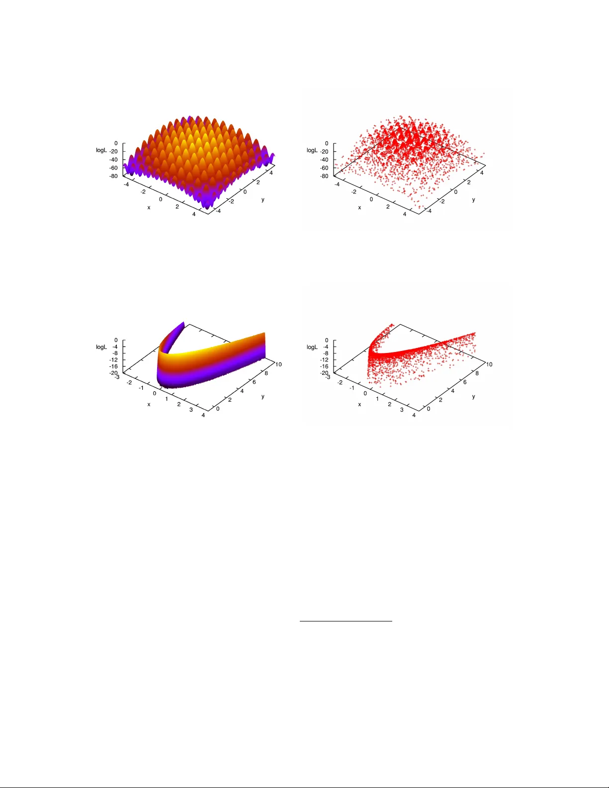
Exploring Multi-Modal Distrib utions with Nested Sampling Farhan Feroz ∗ and John Skilling † ∗ Cavendish Laboratory , Astr ophysics Group, Cambridg e CB3 0HE † Maximum Entr opy Data Consultants, Kenmar e, Ireland Abstract. In performing a Bayesian analysis, two dif ficult problems often emerge. First, in es- timating the parameters of some model for the data, the resulting posterior distribution may be multi-modal or e xhibit pronounced (curving) degeneracies. Secondly , in selecting between a set of competing models, calculation of the Bayesian evidence for each model is computationally ex- pensiv e using existing methods such as thermodynamic integration. Nested Sampling is a Monte Carlo method targeted at the efficient calculation of the evidence, but also produces posterior in- ferences as a by-product and therefore provides means to carry out parameter estimation as well as model selection. The main challenge in implementing Nested Sampling is to sample from a con- strained probability distribution. One possible solution to this problem is pro vided by the Galilean Monte Carlo (GMC) algorithm. W e show results of applying Nested Sampling with GMC to some problems which ha ve prov en very dif ficult for standard Marko v Chain Monte Carlo (MCMC) and down-hill methods, due to the presence of large number of local minima and/or pronounced (curv- ing) degeneracies between the parameters. W e also discuss the use of Nested Sampling with GMC in Bayesian object detection problems, which are inherently multi-modal and require the e valuation of Bayesian evidence for distinguishing between true and spurious detections. Keyw ords: nested sampling, evidence P A CS: 02.50.Tt, 02.60.Jh, 02.70.Rr , 02.70.Uu INTR ODUCTION Bayesian inference provides a consistent approach to the estimation of a set of parame- ters Θ in a model (or hypothesis) H for the data D . Bayes’ theorem states that Pr ( Θ | D , H ) = Pr ( D | Θ , H ) Pr ( Θ | H ) Pr ( D | H ) , (1) where Pr ( Θ | D , H ) ≡ P ( Θ | D ) is the posterior probability distrib ution of the parameters, Pr ( D | Θ , H ) ≡ L ( Θ ) is the likelihood, Pr ( Θ | H ) ≡ π ( Θ ) is the prior , and Pr ( D | H ) ≡ Z is the Bayesian evidence, which is the factor required to normalize the posterior ov er Θ and is gi ven by: Z = Z L ( Θ ) π ( Θ ) d n Θ , (2) where n is the dimensionality of the parameter space. Bayesian e vidence being indepen- dent of the parameters, can be ignored in parameter estimation problems and inferences can be obtained by taking samples from the (unnormalized) posterior distribution using standard MCMC methods. Model selection between two competing models H 0 and H 1 can be done by comparing their respecti ve posterior probabilities gi ven the observ ed data-set D , as follows R = Pr ( H 1 | D ) Pr ( H 0 | D ) = Pr ( D | H 1 ) Pr ( H 1 ) Pr ( D | H 0 ) Pr ( H 0 ) = Z 1 Z 0 Pr ( H 1 ) Pr ( H 0 ) , (3) where Pr ( H 1 ) / Pr ( H 0 ) is the prior probability ratio for the two models, which can often be set to unity in situations where there is not a prior reason for prefering one model over the other , but occasionally requires further consideration. It can be seen from Eq. (3) that the Bayesian e vidence plays a central role in Bayesian model selection. As the av erage of the likelihood o ver the prior , the evidence is lar ger for a model if more of its parameter space is likely and smaller for a model with large areas in its parameter space having low likelihood v alues, e ven if the likelihood function is very highly peaked. Thus, the e vidence automatically implements Occam’ s razor . NESTED SAMPLING Nested sampling [1, 2] is a Monte Carlo technique to estimate the Bayesian evidence by transforming the multi-dimensional evidence integral into a one-dimensional integral. This is accomplished by defining the prior volume X as d X = π ( Θ ) d n Θ , so that X ( λ ) = Z L ( Θ ) > λ π ( Θ ) d n Θ , (4) where the integral extends over the region(s) of parameter space contained within the iso-likelihood contour L ( Θ ) = λ . The e vidence integral, Eq. (2), can then be written as: Z = Z 1 0 L ( X ) d X , (5) where L ( X ) , is a monotonically decreasing function of X . Thus, by e valuating the likelihoods L i = L ( X i ) , where X i is a sequence of decreasing v alues, 0 < X M < · · · < X 2 < X 1 < X 0 = 1 . (6) Evidence can then be approximated numerically using standard quadrature methods as follo ws: Z = M ∑ i = 1 L i w i , (7) where the weights w i for the simple trapezium rule are gi ven by w i = 1 2 ( X i − 1 − X i + 1 ) . The summation in Eq. (7) is performed as follo ws. First N ‘li ve’ points are drawn uniformly from the prior distrib ution π ( Θ ) and initial prior volume X 0 is set to unity . At each subsequent iteration i , the point with lowest likelihood v alue L i is removed from the liv e point set and replaced by another point drawn uniformly from the prior distribution with the condition that its likelihood is higher than L i . This results in the ne w point being drawn uniformly from the prior v olume contained within the iso- likelihood contour defined by L i . The prior volume contained within this region at i th iteration, is a random variable giv en by X i = t i X i − 1 , where t i follo ws the distribution Pr ( t ) = N t N − 1 (i.e., the probability distrib ution for the lar gest of N samples drawn uniformly from the interval [ 0 , 1 ] ). This process is repeated, until the entire prior volume has been trav ersed. The algorithm thus trav els through nested shells of likelihood as the prior v olume is reduced. The mean and standard deviation of log t , which dominates the geometrical exploration, are: E [ log t ] = − 1 / N , σ [ log t ] = 1 / N . (8) Since each v alue of log t is independent, after i iterations the prior volume will shrink do wn such that log X i ≈ − ( i √ i ) / N . Thus, one takes X i = exp ( − i / N ) . GALILEAN MONTE CARLO The main challenge in implementing a nested sampling algorithm is to draw samples from the prior distribution with the constraint L > L i , where L i is lo west likelihood v alue among all live points at each iteration i . One widely used algorithm to approach this problem in astrophysics is MultiNest [3, 4] which is based on an ellipsoidal rejection sampling scheme. At each iteration i , the full set of N liv e points is enclosed within a set of (possibly o verlapping) ellipsoids and a ne w point is then dra wn uniformly from the region enclosed by these ellipsoids. Howe ver , this approach becomes inef ficient in high dimensional ( n & 100) problems. An alternativ e way to draw a point from this constrained distribution is by using MCMC, ho wev er it could be very inefficient in problems exhibiting degeneracies be- tween the parameters. Since we need to draw a point uniformly from the region where L > L i and we already have N ‘liv e’ points distrib uted uniformly inside this region, we could start a Markov Chain at one of these ‘liv e’ points with initial velocity v and reflect off the boundary of this region where L = L i whene ver we encounter it. The problem howe ver is that the location of boundary is not known. Galilean Monte Carlo [5] addresses precisely this problem. At each iteration i , GMC proceeds by picking a ‘liv e’ point with coordinates x 1 at random and gi ves it initial v elocity v . A new point x 2 = x 1 + v is then proposed which is accepted if L ( x 2 ) > L i , otherwise a third point x 3 is proposed by reflecting of f x 2 i.e. x 3 = x 2 + v 0 where v 0 = v − 2 n ( n . v ) and n is a unit vector perpendicular to ∇ L at x 2 . If L ( x 3 ) > L i , x 3 is accepted otherwise the trajectory from x 1 is re versed by gi ving it velocity − v . These mo ves are repeated for k steps resulting in total path length of k v . APPLICA TIONS In this section we show the results of applying Nested Sampling with the GMC algorithm to sev eral multi-modal to y problems which have proven to be very challenging for MCMC algorithms as they tend to get stuck in isolated modes and have very lo w FIGURE 1. Left panel: Himmelblau’ s function with the z-axis being log L ( Θ ) . Right panel: Samples obtained by running GMC algorithm on Himmelblau’ s function. ef ficiencies due to the presence of degeneracies between the parameters. W e refer the reader to [6] for an example of MCMC based algorithms applied to similar problems. In order to analyse these problems with GMC, we used 1000 li ve points and set the log-likelihood log L ( Θ ) = − f ( Θ ) , where Θ = ( θ 1 , θ 2 , · · · , θ n ) is the parameter vector , n is the dimensionality of the problem and f ( Θ ) is the mathematical description of the toy problem. Himmelblau’ s Function Himmelblau’ s function is a 2D function defined as follo ws: f ( x , y ) = ( x 2 + y − 11 ) 2 + ( x + y 2 − 7 ) 2 . (9) It has four identical local minima at ( 3 , 2 ) , ( − 2 . 81 , 3 . 13 ) , ( − 3 . 78 , − 3 . 28 ) and ( 3 . 58 , − 1 . 85 ) where f ( x , y ) = 0. Fig. 1 (left panel) sho ws a plot of the Himmel- blau’ s function with the z-axis being log L ( Θ ) = − f ( Θ ) . GMC algorithm was run on this problem by assuming uniform priors U ( − 5 , 5 ) on both x and y . The algorithm took 120 , 939 likelihood ev aluations and the resultant samples are plotted in Fig. 1 (right panel). Eggbox Function Eggbox function is defined as follo ws: f ( Θ ) = − " 2 + n ∏ i cos  θ i 2  # 5 , (10) where θ i ∈ [ 0 , 10 π ] . Fig. 2 (left panel) shows a plot of the 2D Eggbox function with the z-axis being log L ( Θ ) = − f ( Θ ) . GMC algorithm w as run on this problem by assuming FIGURE 2. Left panel: 2D Eggbox function with the z-axis being log L ( Θ ) . Right panel: Samples obtained by running GMC algorithm on 2D Eggbox function. uniform priors U ( 0 , 10 π ) on parameters θ i . The algorithm took 205 , 534 likelihood e valuations and the resultant samples are plotted in Fig. 2 (right panel). Rastrigin Function Rastrigin function is defined as follo ws: f ( Θ ) = 10 n + n ∑ i = 1  θ 2 i − 10 cos ( 2 π θ i )  , (11) where θ i ∈ [ − 5 . 12 , 5 . 12 ] . This functions has the global minimum at θ i = 0 , ∀ i where f ( Θ ) = 0. Fig. 3 (left panel) sho ws a plot of the 2D Rastrigin function with the z-axis being log L ( Θ ) = − f ( Θ ) . GMC algorithm was run on this problem by assuming uni- form priors U ( − 5 . 12 , 5 . 12 ) on parameters θ i . The algorithm took 215 , 916 likelihood e valuations and the resultant samples are plotted in Fig. 3 (right panel). Rosenbr ock Function Rosenbrock function is defined as follo ws: f ( Θ ) = n − 1 ∑ i = 1  ( 1 − θ i ) 2 + 100 ( θ i + 1 − θ 2 i ) 2  , (12) It has the global minimum at ( θ 1 , θ 2 , · · · , θ n ) = ( − 1 , 1 , · · · , 1 ) where f ( Θ ) = 0. Fig. 4 (left panel) sho ws a plot of the 2D Rastrigin function with the z-axis being log L ( Θ ) = − f ( Θ ) . Because of the presence of thin curving degenerac y , finding the global minimum for this problem is very challenging. GMC algorithm was run on this problem by assuming uniform priors U ( − 20 , 20 ) on parameters θ i . The algorithm took 218 , 982 likelihood e v aluations and the resultant samples are plotted in Fig. 4 (right panel). FIGURE 3. Left panel: 2D Rastrigin function with the z-axis being log L ( Θ ) . Right panel: Samples obtained by running GMC algorithm on 2D Rastrigin function. FIGURE 4. Left panel: 2D Rosenbrock function with the z-axis being log L ( Θ ) . Right panel: Samples obtained by running GMC algorithm on 2D Rosenbrock function. B A YESIAN OBJECT DETECTION W e no w consider the problem of detecting and characterizing discrete objects hidden in some background noise using Nested Sampling with GMC. W e consider our data vector D to be pixel values in the image in which we want to search for these objects. Let us suppose that these objects are described by a template s ( x ; Θ ) , where Θ denotes collecti vely the ( X , Y ) position of the object, its amplitude A and some measure R of its spatial extent. In this e xample we assume spherical Gaussian shaped objects such that: s ( x ; Θ ) = A exp  − ( x − X ) 2 + ( y − Y ) 2 2 R 2  (13) The contribution from each object is assumed to be additiv e. Therefore if there are N ob j such objects present then: D = m + N ob j ∑ k = 1 s ( x ; Θ k ) , (14) 0 2 4 6 8 10 12 x (pixels) y (pixels) 0 50 100 150 200 0 50 100 150 200 -10 -5 0 5 10 15 x (pixels) y (pixels) 0 50 100 150 200 0 50 100 150 200 FIGURE 5. The 200 × 200-pixel test image (left-hand panel) contains 8 Gaussian objects of varying widths and amplitudes; the parameters X k , Y k , A k and R k for each object are listed in T ab. 1. Right-hand panel shows the corresponding data map with independent Gaussian noise added with an rms of 2 units. T ABLE 1. T rue and inferred parameter v alues (with GMC) for X k , Y k , A k and R k ( k = 1 , ..., 8 ) defining the Gaussian shaped objects in Fig. 5. T rue Parameter V alues Inferred Parameter V alues Object X Y A R X Y A R 1 43.7 22.9 10.5 3.3 43.4 ± 0.1 22.8 ± 0.1 11.0 ± 0.4 3.3 ± 0.1 2 101.6 40.6 1.4 3.4 101.7 ± 1.0 41.2 ± 0.9 1.4 ± 0.3 4.1 ± 0.6 3 92.6 110.6 1.8 3.7 92.0 ± 1.3 110.3 ± 1.2 1.4 ± 0.3 4.7 ± 0.9 4 183.6 85.9 1.2 5.1 183.9 ± 1.6 87.0 ± 1.1 1.3 ± 0.3 4.8 ± 0.9 5 34.1 162.5 1.9 6.0 34.0 ± 0.7 163.5 ± 0.8 2.0 ± 0.3 5.4 ± 0.5 6 153.9 169.2 1.1 6.6 152.7 ± 1.1 170.5 ± 1.2 1.5 ± 0.2 6.1 ± 0.5 7 155.5 32.1 1.5 4.1 157.2 ± 1.6 30.4 ± 1.3 1.2 ± 0.3 4.7 ± 0.9 8 130.6 183.5 1.6 4.1 129.3 ± 1.1 183.2 ± 1.3 1.4 ± 0.3 5.0 ± 0.8 where m denotes the generalized noise contrib ution to the data from background emission and instrumental noise and s ( x ; Θ k ) is the contribution to signal from k t h discrete object. W e therefore need to estimate the v alues of unknown parameters ( N ob j , Θ 1 , Θ 2 , · · · , Θ N ob j ) . In order to test GMC on this problem, we simulated 8 objects in 200 × 200 pixel image, with template gi ven in Eq.(13) and parameters listed in T ab . 1. Final image is then created by adding independent Gaussian pixel noise with rms 2 units. The underlying model and simulated data are sho wn in Fig. 5. One would ideally like to infer all the unknown parameters ( N ob j , Θ 1 , Θ 2 , · · · , Θ N ob j ) simultaneously from the data. This howe ver requires any sampling based approach to mov e between spaces of dif ferent dimensionality as the length of the parameter vector depends on the unknown v alue of N ob j . Such techniques are discussed in [7]. Nev erthe- less, due to this additional complexity of variable dimensionality , these techniques are generally extremely computationally intensi ve. A similar problem was analysed in [7] with a single source model and therefore the 0 20 40 60 80 100 120 140 160 180 200 0 20 40 60 80 100 120 140 160 180 200 -85100 -85000 -84900 -84800 -84700 -84600 logL x (pixel) y (pixel) logL FIGURE 6. The set of liv e points, projected into the (X, Y)-subspace, at each successi ve likelihood lev el in the nested sampling in the analysis of the data map in Fig. 5 (right-hand panel) using GMC. parameter space under consideration is Θ = ( X , Y , A , R ) which is four-dimensional and fixed. This doesn’t restrict us to detect only one object as the four -dimensional posterior distribution will ha ve numerous modes, each one corresponding to the location of one of the real or spurious objects in the data. Due to high multi-modality , this represents a v ery dif ficult problem for traditional MCMC methods. [3] adopted the single source model for analysing this problem with the MultiNest implementation of Nested Sampling and showed that all 8 objects can be found very ef ficiently . Results of analysing this problem with GMC implementation of Nested Sampling, with a single source model are sho wn in Fig. 6 in which we plot the ‘li ve’ points, projected into the ( X , Y ) -subspace, at each successi ve likelihood le vel in the Nested Sampling algorithm (above an arbitrary base le vel). Inferred parameter values for each object are listed in T ab . 1. It can be clearly seen that all 8 objects have been identified. The run time with GMC was slightly higher than MultiNest but still orders of magnitude lo wer than MCMC approach used in [7]. A CKNO WLEDGMENTS W e would like to thank Mike Hobson and Stev e Gull for very useful discussions on Nested Sampling. REFERENCES 1. J. Skilling, “Nested Sampling, ” in American Institute of Physics Confer ence Series , edited by R. Fis- cher , R. Preuss, and U. V . T oussaint, 2004, pp. 395–405, URL http://www.inference.phy. cam.ac.uk/bayesys/ . 2. D. Sivia, and J. Skilling, Data Analysis A Bayesian T utorial , Oxford Univ ersity Press, 2006. 3. F . Feroz, and M. P . Hobson, MNRAS 384 , 449–463 (2008), . 4. F . Feroz, M. P . Hobson, and M. Bridges, MNRAS 398 , 1601–1614 (2009), . 5. J. Skilling, “Bayesian computation in big spaces-nested sampling and Galilean Monte Carlo, ” in American Institute of Physics Confer ence Series , edited by P . Goyal, A. Giffin, K. H. Knuth, and E. Vrscay, 2012, vol. 1443 of American Institute of Physics Conference Series , pp. 145–156. 6. Y . Li, V . A. Protopopescu, N. Arnold, X. Zhang, and A. Gorin, Applied Mathematics and Computation 212 , 216–228 (2009). 7. M. P . Hobson, and C. McLachlan, MNRAS 338 , 765–784 (2003), astro- ph/0204457 .