A Statistical Peek into Average Case Complexity

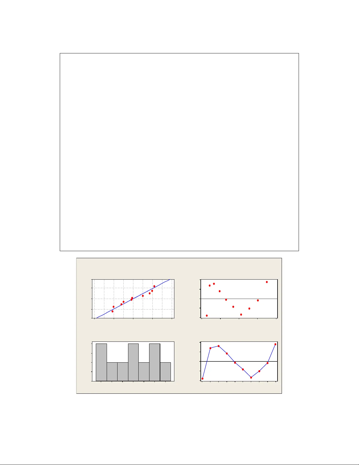
A St a ti st i c a l P e e k i n t o A v e ra g e C a s e C o mp l e x i t y NIRAJ KUMAR SINGH , B irla I nstit ute of Tec hnolog y Mesr a SOUBHIK CHAKR ABOR TY , Birla Institute of Tec hnolog y Me sra DHEERESH KUM AR MALL ICK , Birla Inst itute o f Techno lo gy Me sra The pre sent p aper give s a st atistica l adve nture to wards ex ploring the ave rage c ase c omp lexity behav i or o f compute r algorith ms. Rathe r than fol lowing the tra ditio nal c ount based ana lytic al (pen and pape r) approach, we in stead t alk in te rms o f t he we ight b ased analy sis t hat pe rm its m ixing o f d istinct o per ations into a co nce ptual bou nd ca lled the stati stical bou nd and it s e mp ir ical est im ate, the so ca lled "emp iric al O". Based on care fu l an alysis o f the re sults obt aine d, we have intr odu ce d two new c onje cture s in the do main of algorith mic an alysi s. T he an alytica l w ay o f average c ase an aly sis fal ls flat whe n it co mes to a d ata mode l for which the ex pec tation do es not ex ist (e.g. Cauchy distr ibutio n fo r conti nuou s input d ata a nd ce rta in discrete distribut ion input s as those studie d in the pape r). The empiric al side of our appro ach, with a thrust in co mpute r e xper iments and ap plied stati stic s in its p arad igm, lends a he lpi ng han d by complime nting a nd supple me nting its t heo ret ical co unterp art. C o mputer sc ience i s o r at le ast h as aspects of an e xper imental sc ience as we ll, a nd hence hope fully, our stat istica l fi nding s wi ll be equa lly re c og nized among t heo ret ical scienti sts as well. Key Wor ds: Av erage case analys is, mathemat ical bound, statis tical bound, big-oh , e mpirica l-O, pseudo linear co mplexity , tie-de n sity 1. INTRODUC T ION Traditionally t he analysis of an algorithm ’s effi ciency is done th rough its mathemat ical anal ysis. Alth ough these tec hniques can be a pplied s uccessfull y to many simple algorithms, t he power of mathematics, e ven when enhanced wit h more advanced tech niques , is far from limit less [1][2][3 ]. Rob ustness of the analytical approach itself can be challenged on the ground that even some seemi ngly simple algorithms have proved to be v er y diffic ult to anal yze w ith mathematical precision and certaint y [4]. This is especially true for average case analysis . Average case comple xity analysis is an important idea as it explains h ow certain algorithms with bad w orst c ase complexity p erform bett er on the a ve rage. The principal alternati ve to t he c onventional mathema tical analysis of a n al gorithm’s efficienc y is its empi rical a nalysis [4]. Recently there has been an upswing in i nterest in experime ntal w ork in theo retical c omp uter scienc e community because of growing recognition that theoreti cal results ca nnot tell t he full story abo ut real-world algorithmi c performance [5]. Empirical resear chers have se rious objection to applyi ng mathemat ical bounds in averag e c ase complexity analysis [6] [7] [8]. Indeed , it was the lack of s cientific rigor in early experimental work t hat led Knut h a nd ot her researche rs in the 1960’s to emp hasize worst- a nd- avera ge case analysis and the more general conclusions they could pro vide, especiall y with respect to asymptotic behavior [5]. Empi r ical anal y sis is c apable of fin din g patterns in side a patt ern exhibited by its theoretical counterpart. Its result in turn may reinvi gorate the theoretical establishments by complime n ting and supplementi ng the alr eady known theoretical findings . Here, th rough this paper we s u ggest for an alter n at iv e tool, t h e so c alled ‘ stat istical bound’ and its empiric al estimate (empirical-O) [6] [7]. The performa nc e guarantee is perhaps the biggest strength of the mathematical w orst case bound. Such a guarantee can even be ensured w ith empirical-O (denoted as O emp ) by verifying the complexit y robustness across th e commonly u sed and standard data distrib utions inputs. The statist ical approac h is well equipped with tools a n d te chniques which, if used scientifi cally, can provide a r eliable and valid measure for an algorit hm’s complexit y. See [9] [10] for interesti ng discussi ons on the statis tical analysis of experiments in a r igo r ous fashio n. For more o n statis tical bounds and empirical- O see the Appendi x. Average case inp u ts typicall y correspond to r andomly obtai ned sampl es. Such random seque n ces may constit ute certain well known data patterns or sometimes may even result in unconventional m odels. We in practice a re not v ery mu c h concerned with best c ase analysis as it often paints a very optimistic picture. In this paper we confin e ou r selves to av erage c ase a n alysi s only as w e find it p r acticall y more excit ing than the others. Our statist ical adventure explo r es the a verage ca se behavior of the well kno w n standard qu i ck sort algo rithm [11] as a c ase study. We find it a suitable one as it exhibits a signifi cant performa nce gap betwee n its theoretical ave r age and worst case behaviors. Our analysis introduces a phrase “pseudo linear c omple xity” which w e obtai n against the theoreti c al O(nlog 2 n) complexity for o ur c andida te algorithm . We also talk about t he r ejectio n of t h e average c ase robustness c laim for quick sort algorithm ma de by the the or etical scientists . 2. AVER AG E CASE ANALYS IS US ING S TATIST I CAL B OUND ESTIMATE OR ‘EMP IRI CAL -O’ The av erage case analysis was done by directl y working on pro gram run time to estim ate the weight based stat istical bound over a finite r ange by running c omp uter experiments [12] [13]. This estimat e is called empirical-O. Here time of an oper atio n is taken as its w eight. Weighi n g allows colle ctive considerati on of all ope rations, trivial or non-tri v ial, into a conceptual bound. We c all such a bound a stat istical bound opposed to the tradit ional count based mathemat ical bounds which is operation specific. Since t h e estimate is obtained by supplyi n g nume ric al values to the weights obtained by r unning computer experime n ts, the cr edib ility of this bound estim ate depends on the des ign a nd analysis of comp uter experiment in which ti me is the r espo n se. The interested reader is sug g ested to see [ 6] [14] to g et more insight into stat istical bounds and empiri c al-O. Av erage complexity is traditionall y (by a count based anal ysis u sin g pen a n d paper) fo u nd by appl ying mathematical expectati on to the dominant operation . If th e domi nant operation is wrongl y ch ose n (this is likely in a c omple x code o r even in a simple code in w hich a domi nant operation comes f ewer times as compared to a less dominant op eration which comes more; as for ex ample , in Ami r Schoor’s n-by-n mat rix multiplicat ion algorit hm n 2 comparisons dominat e over multiplicat ions indicati ng an empi r ical O(n 2 ) complexity as the sta tisti cal boun d estima te wh ile Schoor applied mathemat ical expe ctation on multiplicat ion and obtained quite a differe n t r esult , namely, a n average O(d 1 d 2 n 3 ) complexit y, where d 1 a nd d 2 are the fraction of non-zero elements of th e pre and post factor matrices [6][7]. Second, t h e robustness can als o be challenged as the probabili ty distributio n over which expectation is taken may not be realis tic over the problem domain . This section incl udes the empiri c al results obtai ned for average case anal y sis of quick sort algor ithm . The samples are g enerated ran domly, using random number generatin g f unction, to c haracte rize disc r ete u nifor m distribution models with K as its parameter. Our sample sizes lie in between 5*10 5 and 5*10 6 . The discrete uniform distributi on dep en ds on the parameter K [1 …….K], wh i ch is the key to decide the range of sam ple obtained . Most of the mean time entries (in se conds) are aver a ged over 500 trial readin gs. These trial c ounts however, should be varied depending on t he ex te nt of “ noise” present at a pa r ticular ‘n’ value. As a rule of thumb, greater the “noise” at each point of ‘n’, more s h ould be th e numbe r s of obser v ations. System specificatio n: All the c omputer experiments were c arried o ut using PENTIUM 1600 MHz processor and 512 MB RAM. Statis tical models/results are obtai ned using Minitab -15 statist ical package. The standa r d quick so rt is implemented u sing C lan guage by the autho rs thems elves. It should be understood that althou g h program run tim e is system dependent, we a r e interested in ide ntifying patt e rns in t h e run time rather tha n run time itself. It ma y be emph asized here that stati stics is the science of identifying and studying patte rns in numerical data related to some problem u nder stu dy. 2.1 Average case analysis o ver discre te unifor m inpu t s (ca se study - 1) In our first case stud y w e observed the mean times for specific sized input data over the entire ran g e for diffe r ent K values. The obser ved data is recorded in ta ble 1. Table 1. O bs erved m ean t imes i n s e c ond(s) n ↓ K→ 50 500 5000 10000 20000 25000 50 000 50 0000 500000 0 500000 12.688 1.407 0.33104 0.26416 0.2 4652 0.23976 0.24512 0.24276 0.22824 100000 0 50.703 5.219 0.80956 0.57828 0.4 7392 0.45504 0.42136 0.42512 0.42568 150000 0 114.156 11.531 1 .56372 1. 022 56 0.78744 0.75248 0.667 52 0.663 04 0.66576 200000 0 203.546 20.359 2 .57132 1. 616 32 1.18136 1.11132 0.961 84 0.974 36 0.96308 250000 0 317.562 31.657 3 .8498 2.339 48 1.650 08 1.5251 1.3 012 1.30492 1.29804 300000 0 457.797 45.437 5 .3688 3.181 4 2.17812 2. 001 6 1.670 3 1.6 8316 1.66928 350000 0 *** 61.719 7 .156 4.1607 2.76612 2.5157 2.0 859 2.09012 2.08508 400000 0 *** 80.484 9 .187 5.2672 3.4406 3.1045 2.5 217 2.53112 2.53236 450000 0 *** 101.875 11.4323 3 6.5 229 4. 171 88 3.7674 3.0 236 3.0282 3 .01748 500000 0 *** 126.078 13.9326 7 7.8 90333 4.9515 4.4328 3.5342 3.5453 3. 541 88 A caref ul loo k at table 1 reveals that for smaller ‘K’ v alues we get q uadratic complexit y models. Our point is furthe r strength en ed w hen we go throu g h th e stat istical data of tables 2(A-H ). So we can safely write Y avg (n)=O emp (n 2 ), at least for K ≤10000 . It m ust be kept in mind that t he as sociated const ant te rm in this inequality is not a generic one, rather a c onst ant dependent on th e ra n ge of input size. However , if t h e system invariance prope rty of O emp is ensured t hen this v alue may be treated as a constant across t he s y stems provided the range of input size is kept fixed. Table 2(A ) Reg ression Ana lysis: y ver sus n, nlgn, n^2 fo r [k=5 00] The re gre ssion equat ion i s y = - 0.5 41 + 0.0000 13 n - 0.0000 01 nlg n + 0. 0000 00 n^ 2 Predict or Co ef SE Co ef T P Constant - 0.5407 0.365 3 -1. 48 0. 189 n 0 .000 01267 0.00 000 570 2 .22 0. 068 nlgn - 0.000 000 61 0.00 00002 7 -2. 23 0. 067 n^2 0.00 00000 0 0.0 00000 00 62. 14 0.000 S = 0.0 876502 R-S q = 1 00.0 % R-Sq( adj) = 100.0 % Analysi s of V ariance Sourc e DF SS MS F P Regr ession 3 16607 .5 553 5.8 72057 3.28 0.0 00 Residu al Err or 6 0.0 0.0 Total 9 16607 .6 Sourc e DF Se q SS n 1 157 70.1 nlgn 1 80 7.8 n^2 1 2 9.7 Table 2(B ). Regr essio n An alysis: y ver sus n , nlgn for [k= 500] Regress ion Analysis : y versus n, nlgn The re gre ssion equat ion i s y = 19.9 - 0.00 0335 n + 0. 000016 nlgn Predict or Co ef SE C oe f T P Constant 19.927 3.71 2 5.3 7 0 .001 n -0. 000 3349 2 0. 000026 28 -12. 74 0 .000 nlgn 0.00 0015 98 0.0 000011 6 1 3.80 0. 000 S = 2.0 6007 R-S q = 99.8 % R-Sq (adj) = 99. 8% Analysi s of V ariance Sourc e DF SS MS F P Regr ession 2 16577. 9 828 8.9 1953. 16 0. 000 Residu al Err or 7 2 9.7 4.2 Total 9 16607. 6 Sourc e DF Seq SS n 1 1 5770.1 nlgn 1 807.8 Table 2(C ). Regr essio n An alysis: y ver sus n , nlgn, n^ 2 for [k=5 000 ] Regress ion Analysis : y versus n, nlgn, n^2 for [k=50 00] The re gre ssion equat ion i s y = 0.242 - 0.0 0000 3 n + 0.00000 0 nlgn + 0.0 000 00 n^2 Predict or Coe f SE Coe f T P Constant 0. 241 56 0.03 749 6.44 0. 001 n - 0.00 0002 81 0. 0000 0059 - 4.80 0.003 nlgn 0.0 00000 15 0.0 0000 003 5 .24 0.002 n^2 0. 000000 00 0.0000 0000 5 3.27 0.00 0 S = 0.0 089953 9 R-Sq = 100.0% R-S q(adj) = 10 0.0% Analysi s of V ariance Sourc e DF SS MS F P Regr ession 3 1 98.0 24 66 .008 815 749.0 5 0.0 00 Residu al Err or 6 0. 000 0.00 0 Total 9 1 98.0 24 Sourc e DF Seq SS n 1 18 9.642 nlgn 1 8. 153 n^2 1 0. 230 Table 2(D) . Reg ression An alysis : y ver sus n, nlgn, n^2 fo r [k=1 000 0] The re gre ssion equat ion i s y = 0.098 2 - 0. 0000 00 n + 0.0000 00 n lgn + 0. 000 000 n^ 2 Predict or Co ef SE Co ef T P Constant 0 .098 23 0.0 2367 4.1 5 0.0 06 n -0.00 000 019 0. 000000 37 -0. 51 0.6 25 nlgn 0. 000000 02 0.0000 0002 1. 18 0.2 84 n^2 0. 000000 00 0. 0000 0000 47 .33 0.0 00 S = 0.0 056797 9 R-Sq = 100.0% R-S q(adj) = 10 0.0% Analysi s of V ariance Sourc e D F SS MS F P Regr ession 3 61.6 49 20. 550 63699 6.80 0.000 Residu al Err or 6 0. 000 0. 000 Total 9 61.6 49 Sourc e DF Seq SS n 1 59.348 nlgn 1 2.228 n^2 1 0.07 2 Table 2(E ). Regr essio n An alysis: y ver sus n , nlgn, n^ 2 for [k=2 000 0] Regress ion Analysis : y versus n, nlgn, n^2 for [k=20 000] The re gre ssion equat ion i s y = 0.160 - 0.0 0000 2 n + 0.00000 0 nlgn + 0.0 000 00 n^2 Predict or Coe f SE Coe f T P Constant 0.16 047 0.02 249 7.13 0.00 0 n -0 .000 0015 0 0.0 000003 5 -4.2 7 0.00 5 nlgn 0.00 00000 9 0. 00000 002 5.11 0. 002 n^2 0.0 000000 0 0.0 0000 000 21.6 1 0.00 0 S = 0.0 053965 7 R-Sq = 100.0% R-S q(adj) = 10 0.0% Analysi s of V ariance Sourc e D F SS MS F P Regr ession 3 23.4 474 7. 815 8 2683 72.1 9 0.0 00 Residu al Err or 6 0.0 002 0 .0000 Total 9 2 3.44 76 Sourc e DF Seq SS n 1 2 2.8198 nlgn 1 0.6140 n^2 1 0.013 6 Table 2( F). Regr ess ion An alysi s: y versu s n, n lgn, n^2 for [k=2 500 0] The re gre ssion equat ion i s y = 0.129 - 0.0 0000 1 n + 0.00000 0 nlgn + 0.0000 00 n^2 Predict or Co ef SE Co ef T P Constant 0 .129 39 0.0 4199 3.0 8 0.0 22 n -0.00 000 103 0 .000 00066 -1.5 7 0.1 68 nlgn 0. 000000 06 0.0000 0003 2.0 3 0.0 89 n^2 0. 000000 00 0. 000 00000 9.9 8 0.0 00 S = 0.0 100740 R-S q = 1 00.0 % R-Sq( adj) = 100.0 % Analysi s of V ariance Sourc e DF SS MS F P Regr ession 3 1 8.58 35 6. 1945 610 38.16 0.00 0 Residu al Err or 6 0.00 06 0. 000 1 Total 9 18.584 1 Sourc e DF Se q SS n 1 18.14 14 nlgn 1 0.43 20 n^2 1 0.0 101 Table 2(G) . Reg ression An alysis : y ver sus n, nlgn, n^2 fo r [k=5 000 0] The re gre ssion equat ion i s y = 0.178 - 0.0 0000 2 n + 0.00000 0 nlgn + 0.0 000 00 n^2 Predict or Co ef SE Coe f T P Constant 0.17 829 0. 02566 6 .95 0.000 n -0.0 000 0161 0.00 000040 - 4.03 0.00 7 nlgn 0 .00000 009 0.000 00002 4 .75 0 .003 n^2 0.00000 000 0.00 000000 9.05 0.00 0 S = 0.0 061565 9 R-Sq = 100.0% R-S q(adj) = 10 0.0% Analysi s of V ariance Sourc e D F SS MS F P Regr ession 3 11.430 3 3. 8101 1005 21.12 0. 000 Residu al Err or 6 0.00 02 0. 000 0 Total 9 11.430 6 Sourc e DF Seq SS n 1 11.21 28 nlgn 1 0.21 44 n^2 1 0.0 031 Ta ble 2(H). R egressio n Anal ysis: y v ersu s n, nlg n for [k=5 00 00 ] The re gre ssion equat ion i s y = 0.388 - 0.0 0000 5 n + 0.00000 0 nlgn Predict or Co ef SE Coe f T P Constant 0.38 768 0. 03931 9 .86 0 .000 n -0.0 0000 517 0.00 000028 -1 8.57 0 .000 nlgn 0. 000000 26 0 .000 00001 21 .22 0. 000 S = 0.0 218164 R-S q = 1 00.0 % R-Sq( adj) = 100.0 % Analysi s of V ariance Sourc e DF SS MS F P Regr ession 2 1 1.42 72 5 .713 6 12 004.5 3 0.0 00 Residu al Err or 7 0.0 033 0.00 05 Total 9 11.43 06 Sourc e DF Se q SS n 1 11.2 128 nlgn 1 0.214 4 “Even if y ou find a low r 2 value in an analysis , make sure to g o back and look at the regression coefficie nts and their t values. You may find t hat, despite the low r 2 value, one or more of t he regression coefficients is still strong and relat ively well kno wn. In the same man ner, a high r 2 value does n’t n ecessaril y m ean th at the model t h at y ou have fitted to the data is the ri ght model. That is, even when r 2 is very large, t he fitted model may n ot accurately predict the respo n se. It’s the job of lack of fit or goodness of fit tests to decide if a model is a good fit t o the dat a [15]”. Justification for prefer r ing q uadratic mode l over nlog 2 n for K=500: Stat istical data in tables 2(A, B) justify the c hoice of quadratic model ov er nlog 2 n. The standard error is reduced from 2.06007 to 0. 08 76502 when we go for quadratic model. Alt hough a ver y slig h t impro v ement in r 2 data is observed , the F v al ue (7205 73.28) for quadrati c m odel is m u ch higher than t he c orrespondi ng val u e (1953 .16) for nlog 2 n cur ve. Justification for prefer r ing nlo g 2 n mod el over q uadratic on e for K=5000 0: As we move fr om smaller to h igher k values there is a significant gr ad ual dec r ement in t s tatis tic of n 2 te r m which is obvio u s fr om st atis tics given i n tables 2(A -G). Ultima tely for the specified K value the t statis tic of n log 2 n approac hes close to that of n 2 term in t he model. For a g iven r ange of input size (in our case it is 5* 10 5 to 5*10 6 ) an inc rement in K beyond a thres hold (indeed a r ange) ensures its best performance for r andom inputs: i.e. Y avg (n) = O(nlog 2 n). So it is the K value of samp le which decides on the average case behav ior of algorithms (quick sort in partic ular). This information is important as its prior knowledge ma y influe nce the choi ce for a parti cular algorithm i n advan c e. Our study refutes the robustness claim made fo r nlog 2 n av erage c ase beha vior of quick so rt. See r eference [16 ] fo r an i n terestin g dis c ussion o n the robustness of average comple xity meas ur e. 2.2 Average case analysis o ver discre te unifor m inpu t s (ca se study - 2) The frequency of occur rence of a particula r element e i belongin g to a sample is its tie density t d (e i ). As we are dealing with uniform distri bution samples only, to enhanc e the r eadabili ty, we simpl y drop the b r acketed term and hence t d correspo nds to the tie den sity of each eleme n t in the sample. For a n interesting dis c ussion on the effect of tied eleme nts on the al gorithmi c perfo rmance the r eader is re ferred to [1 7]. 2.2.1 Statistica l resu lts and i ts ana l ysis In this section our study is focused around analyzin g algorithmi c pe rforman c e when it is subjected to uniform distributio n data coupled w ith consta nt probabili ty of tied elements. The observed mean time is reco r ded in table 3. The correspo nding stat istical analysis result is pr ese nted in tables 4(A -B). This r esult clearly suggests an O emp (n) com plexit y across the various tie den sit y values. T h e r esulting residual plots for response are given in fig ures 1&2. Table 3 . Obse rve d mean ti mes in sec onds n ↓ t d → 1 10 100 1000 10000 100000 500000 0 .24276 0.24512 0.331 04 1.4 07 12.688 ** * 100000 0 0.4316 0.4283 0.5734 2.7594 25. 219 ** * 150000 0 0.6732 0.664 0. 856 1 4.1281 37 .82 8 * ** 200000 0 0.964 0.9 672 1.1828 5.5125 50.37 5 * ** 250000 0 1.2999 1.2952 1.5062 6.9016 63 * ** 300000 0 1.6767 1.6703 1.7781 8.2842 76. 016 ** * 350000 0 2.0829 2.0859 2.0844 9.7 88.21 9 * ** 400000 0 2.5391 2.5343 2.5391 11.10 433 100.828 ** * 450000 0 3.0219 3.0186 3.0187 12.51 567 113.468 ** * 500000 0 3.54188 3.5 453 3.5342 13.93 267 126.078 *** Table 4(A ). Regr essio n An alysis: t v ersu s n, n log 2 n for t d =1 The re gre ssion equat ion i s t = 0.3 90 - 0.0 00005 n + 0.0000 00 nlogn Predict or Co ef SE Co ef T P Constant 0 .389 54 0.0 4154 9.3 8 0.0 00 n -0.00 000 517 0. 000000 29 -17. 57 0.0 00 nlogn 0. 000000 26 0. 0000 000 1 20. 08 0.000 S = 0.0 230505 R-S q = 1 00.0 % R-Sq( adj) = 100.0 % PRESS = 0.016 428 8 R-Sq(pre d) = 99. 86% Analysi s of V ariance Sourc e DF SS MS F P Regr ession 2 11.44 83 5. 7241 10 773.36 0.000 Residu al Err or 7 0.00 37 0. 000 5 Total 9 11.452 0 Sourc e DF Seq SS n 1 1 1.2341 nlogn 1 0 .214 2 Obs n t Fit SE Fit Res idu al St Resid 1 5000 00 0 .24276 0. 26984 0.019 55 -0 .027 08 -2 .22R 2 100 0000 0 .43160 0. 41036 0.0 1181 0.02 124 1.07 3 150 0000 0 .67320 0. 64910 0.0 1037 0.02 410 1.17 4 200 0000 0 .96400 0. 95163 0.0 1085 0.01 237 0.61 5 250 0000 1 .29990 1. 30158 0.0 1092 - 0.00 168 -0.0 8 6 300 0000 1 .67670 1. 68933 0.0 1025 - 0.01 263 -0.6 1 7 350 0000 2 .08290 2. 10852 0.0 0942 - 0.02 562 -1.2 2 8 400 0000 2 .53910 2. 55461 0.0 0969 - 0.01 551 -0.7 4 9 450 0000 3 .02190 3. 02423 0.0 1225 - 0.00 233 -0.1 2 10 5000 000 3.54 188 3. 514 74 0.0 1702 0.02 714 1.75 R deno tes an o bservat ion w ith a large standard ize d re sidua l. Table 4(B ). Regr essio n An alysis: t v ersu s n, n log 2 n for t d =100 0 Regress ion Analysis : t versus n, nlogn [t d =1 000] The re gre ssion equat ion i s t = 0.1 06 + 0.0 0000 2 n + 0.0000 00 nlogn Predict or Co ef SE Co ef T P Constant 0. 105 638 0.00 830 0 12.7 3 0.000 n 0.0 000 0169 0 .00000 006 28.82 0. 000 nlogn 0.00 000 005 0. 0000 000 0 18.59 0.000 S = 0.0 046060 0 R-Sq = 100.0% R-S q(adj) = 10 0.0% PRESS = 0.000 254 515 R-S q(pred) = 1 00.0 0% Analysi s of V ariance Sourc e DF SS MS F P Regr ession 2 160.10 3 80. 051 37733 04.32 0. 000 Residu al Err or 7 0.0 00 0. 000 Total 9 160.10 3 Sourc e DF Se q SS n 1 1 60.096 nlogn 1 0.00 7 Obs n t Fit SE Fit Res idual St Res id 1 5000 00 1.4070 1.4 082 0.00 39 - 0.0012 -0.51 2 100 0000 2.75 94 2.7 590 0.00 24 0. 0004 0.1 0 3 150 0000 4.12 81 4.1 279 0.00 21 0. 0002 0.0 4 4 200 0000 5.51 25 5.5 087 0.00 22 0. 0038 0.9 4 5 250 0000 6.90 16 6.8 982 0.00 22 0. 0034 0.8 4 6 300 0000 8.28 42 8.2 947 0.00 20 - 0.0105 -2.54R 7 350 0000 9.70 00 9.6 970 0.00 19 0. 0030 0.7 1 8 400 0000 11.1 043 11. 104 3 0.00 19 0. 0000 0.0 1 9 450 0000 12.5 157 12. 516 0 0.00 24 - 0.0003 -0.07 10 5000 000 13.9 327 13. 931 5 0.00 34 0. 0012 0.3 8 R deno tes an o bservat ion w ith a large standard ize d re sidua l. 0 .05 0 0 .02 5 0 .00 0 -0.0 25 -0.0 50 99 90 50 10 1 R e sid u a l Per cent 4 3 2 1 0 0. 030 0. 015 0. 000 -0.0 15 -0.0 30 Fitted Value Resid ual 0. 03 0. 02 0 .01 0. 00 -0.0 1 -0.0 2 -0.0 3 2 .0 1 .5 1 .0 0 .5 0 .0 R e sid u a l Fr e qu e nc y 10 9 8 7 6 5 4 3 2 1 0. 030 0. 015 0. 000 -0.0 15 -0.0 30 O bser v ation O r der Resid ual N ormal P ro b ab il i t y Plo t Versus F i t s Hi st o g ram Versus Ord er Res i du al Pl ots f or y Fig.1. Res idu al plot co rr esponding to t d =1 0.0 10 0 .005 0.0 00 - 0.0 05 -0.0 10 99 90 50 10 1 R e sidu al P er cen t 1 5 1 0 5 0 0.0 05 0.0 00 -0.0 05 -0.0 10 Fitted Va lue Residu al 0 . 0 0 5 0 0 . 0 0 2 5 0 . 0 0 0 0 - 0 . 0 0 2 5 - 0 . 0 0 5 0 - 0 . 0 0 7 5 - 0 . 0 1 0 0 6.0 4.5 3.0 1.5 0.0 R e sidu al Fr eq uenc y 1 0 9 8 7 6 5 4 3 2 1 0.0 05 0.0 00 -0.0 05 -0.0 10 Obser va tion Or der R esidu al N o rm al P ro b ab il it y Plot Versu s F it s Hi st o g ram Vers u s Or d er R es i du al Pl ot s for y Fig.2. Res idu al plot co rr esponding to t d =10 00 With a value of 28.82 the t stat istic is significantly higher for linear term against the value of 18 .59 for nlog 2 n te r m in the lat er model . Opposed to this the t v alue fo r nlog 2 n term (20 .08) is h igher tha n that of linea r term (-17.57) in the ear lie r model. This obse rvation led us to conclude that beyond a threshold value of tie d ensity we expect linea r patterns rat her than nlog 2 n. Pseudo linear complexit y m odel: Analyzing algorithmic complexity through the study of growth patterns is an important idea, but thing s could be different when it comes to p ractice. Unlike theoreti cal anal ysis an empirical analysi s is essentially done ov er a f easible fi nite range. Hence, while going fo r em pirical analysis , o ne should not always r ely c ompletel y o n the growth pat tern as even the individual time values can have thei r own share (sometimes even maj or ) to contribute in deciding t he final complexity of the program in question . A ca reful observat ion of table 3 would further clea r this poi nt. The CPU times a re m or e or less comparable when we look into the columns (table 3) for t d =1, 10, and 100 . Howe v er, as w e moved further for higher t d values, t h e timing differen c es with resp ect to t he CPU times meas u red against the unit t d value became prominent. The tables 1 & 3 are r elated by th e fact that a column in table 3 would corres pond to a rightward diagonal in Table 1 (if all the releva nt entries were present). Each point on an ave rage c omple xity curve, obtaine d for some higher t d (say 1000 as in fig. 3) value, gives a n upper bo und to the corres ponding point (sa mple size) present in some quadratic curve (in fig. 3 these curves correspond to k=5000 and 10000) obtai ned as c omplexit y model f or essentiall y similar inpu t categories. Here we must remember t hat the tie density cannot be an arbitr ary number as it can always be limit ed by the sample size N. Alt hough, the actual timi ngs are c ompared amon g the models obtained from possib ly different data patterns th ey all belong to the very same family of inputs (average c ase i nputs). H en ce, alt hough foll owin g linea r patterns we c all such a model as a “ p s eudo li n ear co mplexity mo d el” . . Fig. 3. Rel ative cur ves de monstr ating pseudo line ar comp lex ity mo del At this point we are in a position to claim that: “ The u niform distribu tion dat a with similar (at least theoretica lly) density of tied e leme nts is g uaranteed to yie ld O emp (n) growth rate ”. In context of theoretical a nalysis this result is quite unexpe cted as even the best c ase theo r etical count happens to be Ω(nlog 2 n) and not a linear one. Based on our anal y sis result we put ou r points in t he form of the followin g two conje c tures. Conjecture 1: Over uniform distrib ution data with simi lar density of tied elements , a theoretical O(nlog 2 n) complexit y approaches to wards an empirical O emp (n) c omple x ity for avera ge case inputs having sufficiently large t d v alues. Conjecture 2: As the sample tie density t d goes beyond a certain threshold v al ue t dt , (i.e. for all t d > t dt ) even the seemi ng ly linear complexity model , as claimed i n conjecture 1, is found to be quadratic in practice, pr ov ided the sample range remains the same. And hence, we call su ch a linear model as “a pseudo li near complexity model”. Although, the presen c e of othe r reasons cann ot be ru led out, our failure in identif ying the dominant operat ion(s), and that too correctly , present inside the c ode is among the reasons fo r the obse r ved beha v ior. Theoretic al justifica tion: It is well known that runtime of quick sort depends on the number of distin ct elements [18], which in this paper, is refle cted in the parameter ‘k’. If t d is the tie den sity , then n=k*t d . With fixed t d , in a feasible finite range setup the v alue of ‘k’ will increase linearly w ith n. The simi lar argume nt is equally applicable for fixed ‘k’ value (see fig. 4 A & B). Also for fixed sample sizes the response is ma ximum wh en t d =n (t d cannot exceed n), whic h is t h e case when all elements are same valued. The response is minimu m when t d =1, (i.e. n=k) wh en all elements are distinct (a t least theoretically) . 0 2 4 6 8 10 12 14 16 5 10 15 20 25 30 35 40 45 50 mean time (T) in sec. input size in lacs (N) Plot of N vs. T K=5000 K=10000 TD=1000 Fig. 4 (A). Line ar p lot of N vs . K Fig. 4(B). Line ar plot of N v s. t d Fig. 5 (A). plot of k v s. mean ti me (t) Fig. 5(B). plot o f t d v s. mean time (t) The expe c ted behavior of a random sample is O (nl og 2 n) complexity whereas , fo r a fixed sample size the run time of quick sort is a dec r easing function over paramet er ‘k’ (see fig. 5 A & B) . This obse rvation affects the r untime of the samp les decreasing the overall ru ntime from n log 2 n comple xity to a li n ea r one. Following this discussion it seems that t he empiric al analysis has the pote ntial to cross the bar rier, w hich ot herwise is n ot atta inable throug h its theo retical counterpa rt. 2.2.2. Q ui ck sort for unusual da ta model : Analyzing the algo r ithmic behavio r , for average case performan ce, t hrough analytical approach has its ow n inherent limita tions as mentioned in t he Introductio n section of this paper. Further these techniques fall flat when the algo rithm is analyzed for some u nusual data set fo r which theoreti cal expect ation does not exists . In such a situat ion the empirical analysis is th e only c h oice. Let u s consider the random v ariab le X w hich takes the discrete values x k = (-1) k 2 k /k, (k=1, 2, 3……. . ), with p r obabili ties p k = 2 -k . Here w e get ∑ (   x k p k ) = ∑ ( − 1 ) ^  /    = - [1- 1/2 + 1 / 3 – 1/4 + …..] = log e 2 and ∑ (   |x k |p k ) = ∑ 1/    which is a div er g ent series. Hence i n this case expectation does not exist . Using the i nverse cdf te c hnique w e have : F X (x) = P( X ≤ x) = ∑  (  =  )   , F X (x) ~ U[0, 1] k → input (N) in lacs → linear plot of N vs. K (fixed t d ) t d → input (N) in lacs → linear plot of N vs. t d (fixed K) mean time (t) in sec. → K → decr easing curve of K v s. me an time (t): N is fixed mean time (t) in sec. → td → increasing curve of t d vs. mean time (t): N is f ixed This unusual data model is simulat ed over various sample ranges w hose regress ion analysis result is given in table (5) and fig. (6). We have used the q u adratic model as a test of linea r /log 2 n goodness of fit. The test is perform ed by fitti ng a quadrati c model to the data: y = b 0 + b 1 x + b 2 x 2 , wh ere the regress ion coefficients b 0 , b 1 , and b 2 are estim ates of the respectiv e parameters. From the r egres sion an d ANOVA tables it is evident that t he r 2 is much h ighe r, the standar d error (S) is smaller . The result of coeffici ent for the v arious terms are n ot informat ive b ut mo re importantly, thei r t values are. The t value for quadratic term is statis tically much significant than the other terms, w hich is an evidence of quadratic nature of the algorithmic behavio r for the said data model . This result again refutes t h e robust ness claim of avera g e case behavior of quick sort al gorithm. Table 5 . Regr ession A nalys is: t ve rsu s n, n log 2 n, n 2 Regress ion Analysis : T versu s N, NlogN , N^2 The re gre ssion equat ion i s T = 0.010 + 0.0 000 34 N - 0.00 0002 Nlog N + 0.0000 00 N^ 2 Predict or Coe f SE Co ef T P Constant 0 .010 0 0. 1024 0.1 0 0.9 25 N 0.0 000344 9 0.0000 3115 1.1 1 0. 311 NlogN -0.0 000021 2 0.0000 0190 -1.1 1 0.308 N^2 0.00 00000 0 0 .00000 000 34.7 9 0.0 00 S = 0.0 245745 R-S q = 1 00.0 % R-Sq( adj) = 100.0 % Analys is of Varian ce Sourc e D F SS MS F P Regr ession 3 412.4 7 137 .49 2276 66.9 3 0.0 00 Residu al Err or 6 0. 00 0.00 Total 9 412.4 7 Sourc e DF Se q SS N 1 391 .67 NlogN 1 20 .07 N^2 1 0.7 3 Obs N T F it SE F it Res idual St R e sid 1 2000 0 0.3057 0.29 90 0.02 34 0.0 066 0.90 2 4000 0 0.9044 0.91 30 0.01 49 -0.00 86 -0.44 3 6000 0 1.8937 1.90 49 0.01 49 -0.01 12 -0.57 4 8000 0 3.2939 3.28 58 0.01 28 0.0 081 0.39 5 10000 0 5.0515 5.06 11 0.01 17 -0.00 96 -0.44 6 12000 0 7.2734 7.23 38 0.01 25 0.0 396 1.87 7 1 4000 0 9.8092 9.80 62 0.01 33 0.0 030 0.15 8 1 6000 0 12. 7451 12.7 796 0.01 27 -0.03 45 -1.64 9 18000 0 16. 1437 16.1 552 0.01 31 -0.01 15 -0.55 10 2 0000 0 19. 9518 19.9 338 0.02 13 0.0 180 1.48 0.050 0.02 5 0.00 0 - 0.02 5 - 0.050 99 90 50 10 1 Res idual Pe rcent 20 15 10 5 0 0.04 0.02 0.00 - 0.02 - 0.04 F it ted V a lue Residu al 0. 04 0 .0 3 0 .0 2 0 .0 1 0. 00 -0 .0 1 -0 .0 2 -0 .0 3 4 3 2 1 0 Res idual Fr equ ency 10 9 8 7 6 5 4 3 2 1 0.04 0.02 0.00 - 0.02 - 0.04 O bser va tio n O r der Resid ual N o r mal P r o b ab i lit y P lo t Ve r su s F it s H i s t o g ram Ver su s Or d er R e s i du al P l ot s f or T Fig.6. Res idu al plot fo r an u nus ual d ata mode l 3. CONCLU SIONS We conclude this pape r with t he following remarks: This r esearch paper ca r efully explores the average case beh avior of our candidate algorithm using the unconventional statis tical bound and its empi rical estimat e, t he so called ‘ empirical -O’. The sta tisti cal bound has surel y m u ch more to offer, as is obvious from our adventure, than its theoretical counterpart . This untraditional and unconventional bou nd (which ac t u ally is a n esti mate [6]) h as the pot entia l to compliment a s well a s supplem ent the fi ndings o f much practi ced math ematical bound. The stat isti cal analysis performed over empi r ical data for discrete un iform distributi on inputs resulted in several practicall y interesti ng patterns. To our surprise we f ound s ome c omple x ity data follo win g a v ery clear linear pat tern suggesting an empi rical linear model, i.e., Y avg = O emp (n). But inte restingly, the proper exami nation of i n dividual response values put a serio u s obj ection on t he validity of this p roposed comple xity model for all practical purposes. These phenomena r es u lted in con je ctures 1 & 2 as g i ven i n the main text of this paper. As the last adven ture of our to u r, we examin ed the behavio r for a non-sta ndard data model for which expectat ion does not exists th eoreticall y. Based on ou r statis tical analysis result, w e h a v e refuted t h e robustness claim of average case behavior of quick sort alg orithm. The general techniques for simulat in g th e conti n uous and discrete as well as uniform and non un iform random v ariables c an be found in [19 ]. For a comprehe n sive literature on sorting, see r eferen ces [1] [20]. F or sor ting with emph asis on the in put distributi on, [21] may be cons ulted. The c on c ept of mixing operations, as is done inheren tly b y experimenta l approa ch, of different t ypes is n ot c ompletel y a new idea. In the w ords of Horo w itz et. al. “Given the mi nimum utility of determini n g the exact number of additions, subtractio ns, and so on, th at are needed to solve a problem instance with characteristics given by n, we might as w ell lump all the operations to g ether (pr ovided that t h e time required b y each is relativel y independent of the instance chara c teristics) and obtain a count for the total nu mbe r of operations” [22]. What is n ew with our approach is that: instead of count we p r efer to w ork w ith w eights and think of a c oncep tual bound based on these w eig h ts, which r elativel y is a mo re scientific approach as it is well known that different operations mi ght take different amou n t of actual CPU times. The role of weighted count becom es more promin en t wh en the operations in c onsid eration differ drasticall y w it h respect to the actual consumed time . The cr edibilit y of the statis tical bound estimate depends on the desi g n a nd anal y sis of our comp uter experime n t in which the respo nse variable is p r ogram run time [6]. Our prime objecti ve behind this paper is to convince its reader about the existence of weight based s tatis tical boun d. We stro n gly reco mmend use of empirical-O for arbitrary algorithms having s ignifica n t pe r forman c e gap, as in th e present case, between t h eir theoreti cal average and worst case bounds. The use of empirical-O is also r ecommended for algorithms in which identif ying the key operation itsel f is a non trivial tas k. Co n cedin g to the fact that the field of count based theoretical analysis is quit e satu rated now, h opefull y t h e c omm unity of theoreti c al computer scientists would find our app r oach a systemat ic and scientifi c one, and hence would appreciate our stati stical findings. APPE NDIX Definition: Stat istical bound (no n-probabilis tic) If w ij is th e weight of (a c omp uting) operation of type i in the j th repetition (generally time is taken as a weig ht) and y is a “stoc h astic realizat ion” (which ma y not be stochasti c [6]) of the determi n istic T=  1 . w ij wh ere we count one for each opera ti on repetition irrespecti v e of the type, the stat istical bound of the algorithm is the asymptot ic least upper bound of y expressed as a fu nction of n where n is t he input parameter c haracterizin g the algo rithm’s i n put size. If i n terpreter is u sed, t he measured time will involve both the t r anslation tim e and the ex ecutio n time but the translati on time being indepen dent of the input will not affe c t the order of complexit y. The deter mi n istic m odel in that c ase is T=  1. w ij + translat ion time. For parallel comp uting, summat ion should be replaced by maxim um. Empirica l O (written as O w ith a s u bscript emp) is a n empirical estimate of t he statis tical boun d over a finite range, obta in ed b y suppl y ing numerica l values to the w eights, which emerge from c omputer experiments [6]. Empirical O can als o be used to estimat e a mathem atical bound w hen t h eoretical analysis is tedious, w ith the ackno wledgeme n t that in this case the estim ate shou ld be count based a nd operation specifi c. REFE RENC ES [1] R. Sedg ewick , and P. F lajolate . 1 996. A n Introd uction to the Analysis of Algorit hm s. A dd ison-We sley , Reading, MA [2] Grah am, R .L., Knuth, D .E., and Pat ashnik, O. 1994. Co ncre te Mathematics: A Fo undatio n for Compute r Scie nce, 2 nd ed. Addiso n- Wesley, Re ading, MA [3] D. H. Gr ee n, and D . E. K nuth. 1982. Mathem atic s for A nalysis of A lgorith ms, 2 nd e d. Birk hause r, Bosto n [4] A. Lev itin. 2009. I ntro duction to the e sign & An alysi s of Algor ithms . 2 nd ed. , Pear son Educ ation [5]Dav id S. John son. Nov 2001. A Theo re tician’s G uide to the Exper imental An alysi s of Algorit hm s. http://www.r esear ch att.com/ ~dsj/ [6] So u bhik C hakra bor ty and S um an Ku mar So urabh. 2010. A C omputer E xper ime nt O riente d Appro ach to Algo rithmic Co mp lexity. La mbert Acade mic Pub lish ing [7] Su man Ku mar S our ab h a nd S ou bhik C hakr abo rty. 200 7. On Why Algo rith mic Ti me C omp lexity Measure C an be Syste m Invari ant R athe r than System Indepe ndent. Applie d M athem atic s and Computat ion, Vo l. 190, Is sue 1, 195-2 04 [8] Sou bhik C hak ra borty . 201 0. Rev iew of t he B oo k Me thods in Algo rithmic Analy sis by V. Do bru shkin. Chapma n and Hall, P ub lished in Co m puting R eview s, Ju ne 1 1, 2010 [9] Co ffi n. 2000 . Statist ica l a nalys is of comp utat iona l te st s of algor ithms and heurist ics. Info rms J. on Computi ng [10] C. Co tt a, and P. Mosc ato. 2 003. A Mixe d Evo lutionary -Statist ical An alysis of an Algo rithm’s Complexity . App lied M athem atic s Lette rs, 16, 41-4 7 [11] C. A. R. Ho are. 1962. Q uick sort . Computer Jo urnal, 5(1), 10-1 5 [12] Jero me Sacks et al. 19 89. Design and A na lysis o f Expe rimen ts. Stat istical S cience , V ol . 4, No. 4, 40 9- 423 [13] K . T. Fa ng, R. Li, and A. S udji anto. 20 06. De sign and Mo del ing o f Comp ute r Expe riments . Ch ap man and H all [14] N iraj K um ar S ingh and Soubhik C hak raborty . 2011. Part i tion So rt and its Empirica l Analys is. In Proc ee dings o f the Internat ional Confe re nce o n Com putat io nal Intelligenc e and Info rmat ion Techno logy (CI IT 20 11). CC IS 2 50, 34 0-346 . © Spr inger-V erlag He idelberg 201 1 [15] Paul Mathe ws. 20 10. De sign o f E xper ime nts w ith M INITAB . Ne w Age Internat iona l Pu bl isher s, F irst Indian Su b-Co ntine nt Ed ition, 2 94 [16] Soub hik Ch akr aborty and S uma n K umar Sour abh. 20 07. How R obu st are Av er age Com plexity Measures? A St atist ical Ca se St udy. A pplied Mathe mat ics and Co mput ation, 1 89, 1 787- 1797 [17] Soub hik C hakra bor ty, Su man Ku mar So ur abh, M. Bose, a nd K umar S usha nt. 20 07. Rep lace ment So rt Revisited: “ The Gold St and ard U neart hed!”. App lied Mat hem atics and Co mput ation, 1 89, 384-394 [18] R. Sed gew ick. June 1977. Qu ick sort w ith Equ al Ke ys. Sico mp 6(2), 240-2 67 [19] S. Ros s. 2001. A F irst Co ur se in Pr obabi lity, 6 th E ditio n. Pe arson Educ ation [20] Dona ld E. K nuth. 2000. The Art of Computer Pro gr amming , Vo l. 3: Sor ting a nd Se arching . Ad dison Wesely, Pearson E duc at ion Repr int [21] H. M ahmo ud. 2 000. Sor ting : A D istribut ion Theo ry. John Wil ey and Son s [22] E llis Hor owitz, S. S ah ni, and S. R ajasekar an. 2 013(Re print) . Fund ament al s o f C omp uter A lgorith ms. 2 nd ed., U niversity Pre ss