Nonasymptotic bounds on the estimation error of MCMC algorithms

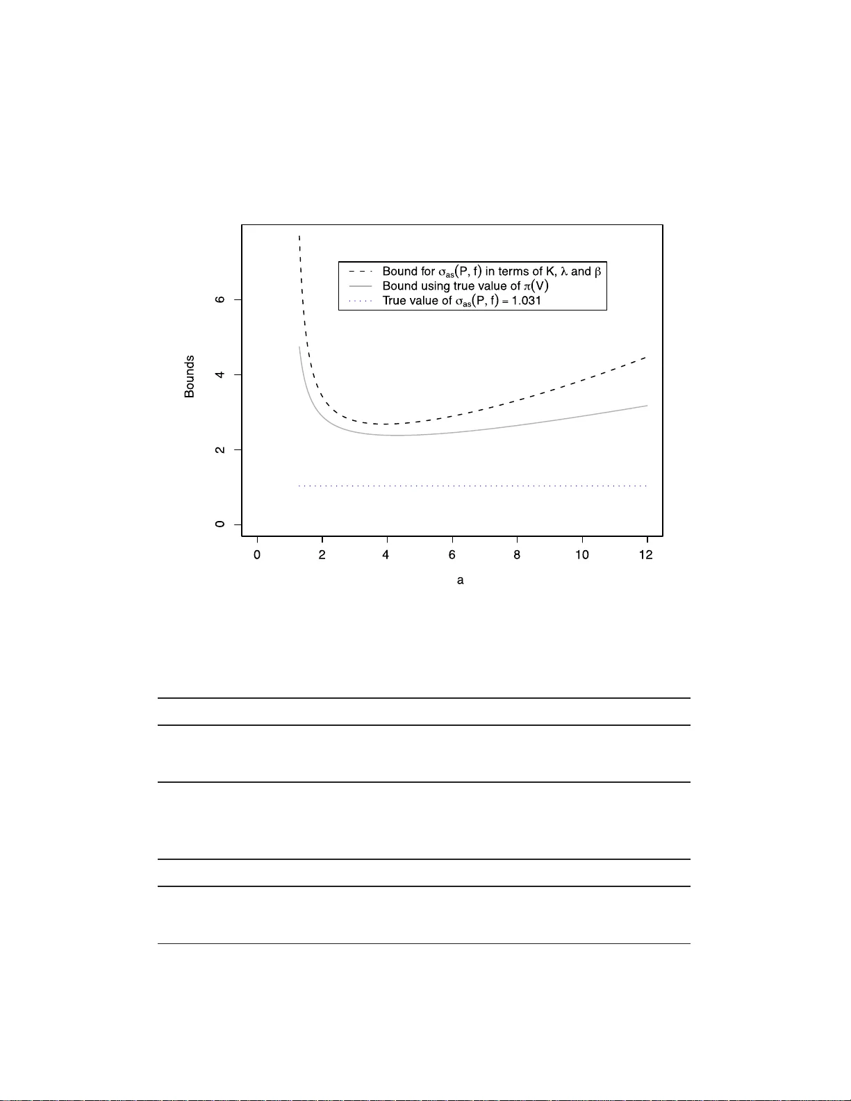
Bernoul li 19 (5A), 2013, 2033–206 6 DOI: 10.315 0/12-BEJ 442 Nonasymptotic b ounds on the estimation error of MCMC algorithms KRZYSZTOF LA TUSZY ´ NSKI 1 , B lA ˙ ZEJ MIASOJEDOW 2 and W OJCIECH NIEMIR O 3 1 Dep artment of Statistics, University of Warwick, CV4 7AL, Coventry, UK. E-mail: latuch@gmail.c om ; url: http://www.warwick.ac.uk/go/klatusz ynski 2 Institute of Applie d Mathematics and Me chanics, Uni vers ity of Warsaw, Banacha 2, 02-097 Warszawa, Poland. E-mail: bmia@mimuw. e du.pl 3 F aculty of Mathematics and Computer Scienc e, Ni c olaus C op ernicus U ni ver sity, C hopina 12/18, 87-100 T oru ´ n, Pol and. E-mail: wniem@mat.uni.torun.pl W e address the problem of upp er b ounding th e mean square error of MCMC estimators. Our analysis is nonasymptotic. W e first establish a general result v alid for essentiall y all ergo dic Mark o v c hains encountered in Bay esian compu tatio n and a p ossi bly unb ou n ded target func- tion f . The b ound is sharp in th e sense that the leading term is exactly σ 2 as ( P , f ) /n , where σ 2 as ( P , f ) is the CL T asympt otic v ariance. Next, we pro ceed to sp ecific ad d itional assumptions and g ive explicit compu table b ounds for geometrically and polynomially ergodic Marko v chai ns under q uan titativ e d rif t conditions. As a corollary , w e pro vide results on confiden ce estimation. Keywor ds: asymp totic v ari ance; computable b ounds; confidence estimation; drift cond itio ns; geometric ergodicity; mean square error; polynomial ergo dicit y; regeneration 1. In tro duction Let π b e a probability distribution on a P olish space X and f : X → R be a Bor el function. The o b jectiv e is to compute (estimate) the q uan tit y θ := π ( f ) = Z X π (d x ) f ( x ) . Typically X is a high dimensio nal s pace, f ne ed not b e b ounded a nd the density of π is known up to a normalizing constant. Such pr oblems a rise in Bay esian infer ence and ar e often solved using Markov chain Mont e Car lo ( MCMC) metho ds. The idea is to simulate a Ma rk ov chain ( X n ) with transition kernel P such that π P = π , that is π is sta tionary This is an electronic reprint of the original article published by the ISI/BS in Bernoul li , 2013, V ol. 19, No. 5A, 2033–2066 . This reprint differs from the original in pagination and typographic detail. 1350-7265 c  2013 ISI/BS 2 K. Latu szy´ nski, B. Miasoje dow and W. Niemir o with resp ect to P . Then av erages a long the tra jector y o f the chain, ˆ θ n := 1 n n − 1 X i =0 f ( X i ) are used to estimate θ . It is essential to have ex plicit and reliable b ounds which pr o vide information ab out how long the a lgorithms must be run to achiev e a pre scribed level of accuracy (cf. [ 28 , 29 , 53 ]). The aim of our paper is to der iv e no nasymptotic and explicit bo unds on the mean sq uare error , MSE := E ( ˆ θ n − θ ) 2 . (1.1) T o uppe r b ound ( 1.1 ), we be gin with a general inequality v alid for all ergo dic Ma rk ov chains that a dmit a o ne step s mall set condition. Our b ound is sharp in the sense that the leading term is exactly σ 2 as ( P, f ) /n , where σ 2 as ( P, f ) is the asy mptotic v aria nce in the central limit theore m. The pro of relies o n the regeneration t echnique, metho ds of renew al theory and sta tistical sequential analys is. T o obtain explicit b ounds, we subsequently consider g eometrically a nd p olynomially ergo dic Ma rk ov chains. W e assume appro priate drift conditions that give quantitativ e information ab out the transition kernel P . The upp er bounds o n MSE a re then s tated in terms of the drift para meters. W e note tha t most MCMC algo rithms implemen ted in Bay esian inference are geomet- rically or p olynomially ergo dic (how ev er establishing the quan titativ e drift conditions we utilize may b e pro hibitiv ely difficult for co mplicated mo dels). Uniform er godicity is stronger then geometrical er godicity co nsidered h ere and is often discussed in litera- ture. Howev er, few MCMC algorithms used in practice are uniformly ergo dic. MSE and confidence es timation for unifor mly ergo dic chains are discus sed in our a ccompan ying pap er [ 34 ]. The Subgeometr ic condition, considered in, for exa mple, [ 1 0 ], is more g eneral than po lynomial ergo dicity consider ed her e. W e note that with some additional effor t, the results for p olynomially ergo dic c hains (Section 5 ) can b e r eform ulated for s ubgeometric Marko v c hains. Motiv ated by applications, we av oid these technical difficulties. Upper b ounding the mea n squa re erro r ( 1.1 ) leads immediately to confidence estima- tion by applying the Chebyshev inequality . O ne can also apply the more sophis ticated median trick of [ 25 ], further dev elop ed in [ 45 ]. The median trick leads to a n exp onen- tial inequa lit y for the MCMC estimate whenever the MSE can b e upp er b ounded, in particular in the setting of geometrically and p olynomially ergo dic chains. W e illustrate our res ults with b enc hmark examples. T he first, which is related to a simplified hie rarchical Ba y esian mo del a nd similar to [ 29 ], E xample 2, allows to co mpare the b ounds provided in our pap er with a ctual MCMC err ors. Nex t, we demonstra te how to apply our results in the Poisso n–Gamma mo del of [ 18 ]. Finally , the contracting normals to y-example a llo ws for a n umerical compar ison with our ea rlier work [ 35 ]. The pap er is o rganised as follows: in Section 2 we give bac kground on the regenera tion techn ique and introduce no tation. The general MSE upp er bo und is derived in Section 3 . Nonasymptotic estimation err or of MCMC 3 Geometrically and p olynomially ergo dic Marko v chains are consider ed in Sections 4 and 5 , resp ectiv ely . The applicability of o ur results is discusse d in Section 6 , where also numerical examples are pres en ted. T ec hnical pr oofs are deferred to Sections 7 and 8 . 1.1. Related nonasymptotic results A v ast literature o n nona symptotic a nalysis o f Ma rk ov chains is av ailable in v arious settings. T o place our results in this context, we g iv e a br ief account. In the ca se of finite state sp ac e , an approa c h based on the sp ectral decomp osition was used in [ 2 , 19 , 36 , 45 ] to derive re sults of r elated type. F or b ounde d functionals of uniformly ergo dic ch ains on a general state space, exp onen- tial inequalities with explic it constants s uc h a s thos e in [ 20 , 33 ] can b e applied to der iv e confidence bo unds. In the accompa n ying pa per [ 34 ], we compare the simulation cost of confidence estimation based o n our a pproac h (MSE bo unds with the median trick) to exp onen tial inequalities and conclude that while exp onent ial inequalities hav e sha rper constants, our approach giv es in this setting the o ptimal dependence on the reg eneration rate β a nd therefore will turn o ut more efficien t in ma n y practical examples. Related res ults co me also from studying concentration of measur e pheno menon for depe nden t random v ariables. F or the larg e b o dy of work in this a rea see, for example, [ 40 , 58 ] and [ 32 ] (and references therein), where transp ortation inequalities or martingale approach have b een used. These results, motiv ated in a more general setting, are v alid for Lipschitz functions with resp ect to the Hamming metric. They also include ex pressions sup x,y ∈X k P i ( x, · ) − P i ( y , · ) k tv and when applied to our s etting, they a re well suited for b oun de d functionals of un if ormly ergo dic Ma rk ov chains, but ca nnot b e a pplied to geometrically ergo dic chains. F or details, w e refer to t he orig inal pap ers a nd the discussion in Section 3.5 of [ 1 ]. F or la zy re v ersible Markov chains, nonasymptotic mean square erro r b ounds hav e bee n obtained for b ounde d ta rget functions in [ 57 ] in a setting w here explicit b ounds on conductance are av ailable. These re sults have b een a pplied to a ppro ximating integrals ov er balls in R d under some regular it y conditions for the stationary measure, see [ 57 ] fo r details. The Mar k o v chains considered there ar e in fac t uniformly ergo dic, ho wev er in their setting the reg eneration ra te β , can b e verified for P h , h > 1 rather then for P and turns out to be exp onen tially small in dimension. Hence, conductance se ems to be the natural approach to make the problem tractable in hig h dimensions. T ail inequalities for b ounde d functionals of Markov c hains that a re not uniformly er- go dic were considered in [ 1 , 7 ] and [ 10 ] using r egeneration tec hniques. These r esults apply for example, to ge ometric al ly or s ub ge ometric al ly ergo dic Mar k o v chains, how ev er they also inv olv e nonexplicit consta n ts o r r equire tractability o f moment conditions o f ran- dom tours b et w een r egenerations. Co mputing explic it b ounds fro m these r esults may b e po ssible with additional w ork, but w e do not pursue it her e. Nonasymptotic analysis of unb ounde d functionals of Marko v chains is scarce. In partic- ular, t ail inequalities for unb ounde d target f unction f tha t can be applied to ge ometric al ly ergo dic Mar k o v chains hav e b een established by Bertail and Cl´ emen¸ con in [ 6 ] by regen- erative appro ac h and using tr uncation a rgumen ts. How ever, they inv olve nonexplicit 4 K. Latu szy´ nski, B. Miasoje dow and W. Niemir o constants and ca n not b e directly applied to confidence e stimation. Nona symptotic a nd explicit MSE bounds for ge ometrically ergo dic MCMC samplers have be en obtained in [ 35 ] under a geo metric drift condition by exploiting co mputable conv ergence ra tes. Our present pa per improves these results in a fundamen tal way . Firstly , the generic Theo - rem 3.1 allows to extend the approach to different class es of Marko v chains, for example, po lynomially ergo dic in Section 5 . Se condly , rather then resting on computable conv er- gence rates, the present approach relies on upper-b ounding the CL T asymptotic v ariance which, somewhat surpris ingly , app ears to be more accurate and consequently the MSE bo und is m uch sharp er, as demonstrated by nu merical examples in Sec tion 6 . Recent work [ 31 ] address er ror estimates for MCMC a lgorithms under p ositiv e cur v a- ture condition. The p ositive curv ature implies geometric ergo dicity in the W asser stein distance and biv ariate drift conditions (cf. [ 49 ]). Their a pproach app ears to b e applicable in different settings to ours a nd als o r ests on different notions, fo r ex ample, employs the coarse diffusion consta n t instea d of the exa ct a symptotic v ar iance. Moreov er, the tar - get function f is a ssumed to b e Lipschitz which is problematic in Bay esian inference. Therefore, our r esults and [ 31 ] a ppear to b e complementary . Nonasymptotic rates of conv ergence of geometr ically , p olynomially and subgeo metri- cally er godic Ma rk ov chains to their stationary distributio ns hav e been inv estigated in many pap ers [ 4 , 11 – 13 , 16 , 30 , 43 , 51 , 52 , 5 4 , 5 5 ] under assumptions similar to our Sec- tion 4 and 5 , together with an ap eriodicity condition that is no t needed for our purp oses. Such re sults, although of utmost theoretical impo rtance, do no t directly translate into bo unds on accuracy of estimation, as they allow to control only the bias o f estimates and the so-called bur n-in time. 2. Regeneratio n construction and notation Assume P has inv ariant distribution π on X , is π -ir reducible and Harr is recurre n t. The following o ne s tep small set Ass umption 2.1 is verifiable for virtually all Markov chains targeting Bayesian p osterior distributions. It allows for the regenera tion/split construc- tion o f Nummelin [ 46 ] and A threya and Ney [ 3 ]. Assumption 2.1 (Smal l set). Ther e exist a Bor el set J ⊆ X of p ositive π me asu r e, a numb er β > 0 and a pr ob abili ty me asur e ν such t hat P ( x, · ) ≥ β I ( x ∈ J ) ν ( · ) . Under Ass umpt ion 2.1 , we can define a biv ariate Mar k o v chain ( X n , Γ n ) on the spa ce X × { 0 , 1 } in the following wa y . Bell v ariable Γ n − 1 depe nds only on X n − 1 via P (Γ n − 1 = 1 | X n − 1 = x ) = β I ( x ∈ J ) . (2.1) The r ule of transition from ( X n − 1 , Γ n − 1 ) to X n is g iv en by P ( X n ∈ A | Γ n − 1 = 1 , X n − 1 = x ) = ν ( A ) , P ( X n ∈ A | Γ n − 1 = 0 , X n − 1 = x ) = Q ( x, A ) , Nonasymptotic estimation err or of MCMC 5 where Q is the nor malized “res idual” kernel g iv en by Q ( x, · ) := P ( x, · ) − β I ( x ∈ J ) ν ( · ) 1 − β I ( x ∈ J ) . Whenever Γ n − 1 = 1 , the chain regenera tes at moment n . The regenera tion ep o c hs are T := T 1 := min { n ≥ 1: Γ n − 1 = 1 } , T k := min { n ≥ T k − 1 : Γ n − 1 = 1 } . W rite τ k := T k − T k − 1 for k = 2 , 3 , . . . a nd τ 1 := T . Random blo c ks Ξ := Ξ 1 := ( X 0 , . . . , X T − 1 , T ) , Ξ k := ( X T k − 1 , . . . , X T k − 1 , τ k ) for k = 1 , 2 , 3 , . . . are independent. W e note that n um ber ing of the b ell v aria bles Γ n may differ betw een authors : in our notation Γ n − 1 = 1 indica tes regeneration at momen t n , no t n − 1. Let symbols P ξ and E ξ mean that X 0 ∼ ξ . Note also that these symbols are unam biguous, because sp ecifying the distribution of X 0 is equiv ale n t to spe cifying the joint distribution of ( X 0 , Γ 0 ) via ( 2.1 ). F o r k = 2 , 3 , . . . , every blo ck Ξ k under P ξ has the same dis tribution a s Ξ under P ν . How ev er, the distribution of Ξ under P ξ is in genera l different. W e will also use the following notations for the blo c k s ums: Ξ( f ) := T − 1 X i =0 f ( X i ) , Ξ k ( f ) := T k − 1 X i = T k − 1 f ( X i ) . 3. A general inequalit y for the MSE W e ass ume that X 0 ∼ ξ a nd thus X n ∼ ξ P n . W rite ¯ f := f − π ( f ) . Theorem 3.1. If Assumption 2.1 holds, then q E ξ ( ˆ θ n − θ ) 2 ≤ σ as ( P, f ) √ n  1 + C 0 ( P ) n  + C 1 ( P, f ) n + C 2 ( P, f ) n , (3.1) wher e σ 2 as ( P, f ) := E ν (Ξ( ¯ f )) 2 E ν T , (3.2) C 0 ( P ) := E π T − 1 2 , (3.3) C 1 ( P, f ) := q E ξ (Ξ( | ¯ f | )) 2 , (3.4) 6 K. Latu szy´ nski, B. Miasoje dow and W. Niemir o C 2 ( P, f ) = C 2 ( P, f , n ) := v u u t E ξ I ( T 1 < n ) T R ( n ) − 1 X i = n | ¯ f | ( X i ) ! 2 , (3.5) R ( n ) := min { r ≥ 1: T r > n } . (3.6) R emark 3. 2. The b ound in Theorem 3.1 is meaning ful o nly if σ 2 as ( P, f ) < ∞ , C 0 ( P ) < ∞ , C 1 ( P, f ) < ∞ and C 2 ( P, f ) < ∞ . Under Assumption 2.1 , we alwa ys have E ν T < ∞ but not necessarily E ν T 2 < ∞ . On the other ha nd, finiteness o f E ν (Ξ( ¯ f )) 2 is a sufficient and nece ssary condition for the CL T to hold for Markov chain X n and function f . This fact is prov ed in [ 5 ] in a mor e gene ral setting. F or our purp oses, it is imp ortant to note that σ 2 as ( P, f ) in Theorem 3.1 is indeed the asymptotic varianc e which app ears in the CL T, that is √ n ( ˆ θ n − θ ) → d N(0 , σ 2 as ( P, f )) . Moreov er, lim n →∞ n E ξ ( ˆ θ n − θ ) 2 = σ 2 as ( P, f ) . In this sense, the leading term σ as ( P, f ) / √ n in Theor em 3.1 is “a symptotically corr ect” and ca nnot b e improved. R emark 3.3. Under additional assumptions of geometr ic and p olynomial ergo dicit y , in Sections 4 a nd 5 r espectively , we w ill derive b ounds for σ 2 as ( P, f ) and C 0 ( P ) , C 1 ( P, f ) , C 2 ( P, f ) in terms of some explicitly computable q uan tities. R emark 3.4. In our related work [ 34 ], we d iscuss a special case of the setting considered here, namely when regenera tion times T k are identifiable. These lea ds to X 0 ∼ ν and an regenera tiv e estimator of the form ˆ θ T R ( n ) := 1 T R ( n ) R ( n ) X i =1 Ξ i ( f ) = 1 T R ( n ) T R ( n ) − 1 X i =0 f ( X i ) . (3.7) The es timator ˆ θ T R ( n ) is somewhat easier to analyze. W e r efer to [ 34 ] for deta ils. Pro of of Theorem 3.1 . Recall R ( n ) defined in ( 3.6 ) a nd let ∆( n ) := T R ( n ) − n. In words: R ( n ) is t he first moment of r e gener ation p ast n and ∆( n ) is the oversho o t or excess over n . Let us express the estimatio n error as follo ws. ˆ θ n − θ = 1 n n − 1 X i =0 ¯ f ( X i ) = 1 n T R ( n ) − 1 X i = T 1 ¯ f ( X i ) + T 1 − 1 X i =0 ¯ f ( X i ) − T R ( n ) − 1 X i = n ¯ f ( X i ) ! =: 1 n ( Z + O 1 − O 2 ) , Nonasymptotic estimation err or of MCMC 7 with the co n v en tion that P u l = 0 whenever l > u . The triangle ine qualit y entails q E ξ ( ˆ θ n − θ ) 2 ≤ 1 n ( q E ξ Z 2 + q E ξ ( O 1 − O 2 ) 2 ) . (3.8) Denote C ( P , f ) := p E ξ ( O 1 − O 2 ) 2 and co mpute C ( P , f ) = E ξ ( T − 1 X i =0 ¯ f ( X i ) − T R ( n ) − 1 X i = n ¯ f ( X i ) ! I ( T ≥ n ) + T − 1 X i =0 ¯ f ( X i ) − T R ( n ) − 1 X i = n ¯ f ( X i ) ! I ( T < n ) ) 2 ! 1 / 2 ≤ E ξ T − 1 X i =0 | ¯ f ( X i ) | + T R ( n ) − 1 X i = n | ¯ f ( X i ) | I ( T < n ) ! 2 ! 1 / 2 (3.9) ≤ v u u t E ξ T − 1 X i =0 | ¯ f ( X i ) | ! 2 + v u u t E ξ T R ( n ) − 1 X i = n | ¯ f ( X i ) | I ( T < n ) ! 2 = C 1 ( P, f ) + C 2 ( P, f ) . It re mains to b ound the middle term, E ξ Z 2 , which clearly corre sponds to the mo st significant p ortion of the estimatio n error . The cr ucial step in our pro of is to show the following inequality: E ν T R ( n ) − 1 X i =0 ¯ f ( X i ) ! 2 ≤ σ 2 as ( P, f )( n + 2 C 0 ( P )) . (3.10 ) Once this is prov ed, it is easy to see that E ξ Z 2 = n X j =1 E ξ ( Z 2 | T 1 = j ) P ξ ( T 1 = j ) = n X j =1 E ν T R ( n − j ) − 1 X i =0 ¯ f ( X i ) ! 2 P ξ ( T 1 = j ) ≤ n X j =1 σ 2 as ( P, f )( n − j + 2 C 0 ( P )) P ξ ( T 1 = j ) ≤ σ 2 as ( P, f )( n + 2 C 0 ( P )) , consequently , p E ξ Z 2 ≤ √ nσ as ( P, f )(1 + C 0 ( P ) /n ) and the conclusion will follow b y re- calling ( 3.8 ) and ( 3.9 ). W e are therefor e left with the task o f proving ( 3.10 ). This is e ssen tially a statement ab out sums of i.i.d. r andom v a riables. Indeed, T R ( n ) − 1 X i =0 ¯ f ( X i ) = R ( n ) X k =1 Ξ k ( ¯ f ) (3.11) 8 K. Latu szy´ nski, B. Miasoje dow and W. Niemir o and all the blo c ks Ξ k (including Ξ = Ξ 1 ) a re i.i.d. under P ν . B y the genera l version of the Kac theore m ([ 42 ], Theorem 10.0.1, o r [ 47 ], equation (3.3.7)), w e hav e E ν Ξ( f ) = π ( f ) E ν T (and 1 / E ν T = β π ( J )), s o E ν Ξ( ¯ f ) = 0 and V ar ν Ξ( ¯ f ) = σ 2 as ( P, f ) E ν T . Now w e will exploit the fac t that R ( n ) is a stopping time with res pect to G k = σ ((Ξ 1 ( ¯ f ) , τ 1 ) , . . . , (Ξ k ( ¯ f ) , τ k )), a filtration genera ted by i.i.d. pairs. W e are in a p osition to apply the tw o W ald’s iden- tities. The seco nd ident it y yields E ν R ( n ) X k =1 Ξ k ( ¯ f ) ! 2 = V ar ν Ξ( ¯ f ) E ν R ( n ) = σ 2 as ( P, f ) E ν T E ν R ( n ) . But in this expression, w e can replace E ν T E ν R ( n ) by E ν T R ( n ) bec ause of the fir st W ald’s ident it y: E ν T R ( n ) = E ν R ( n ) X k =1 τ k = E ν T E ν R ( n ) . It follows that E ν R ( n ) X k =1 Ξ k ( ¯ f ) ! 2 = σ 2 as ( P, f ) E ν T R ( n ) = σ 2 as ( P, f )( n + E ν ∆( n )) . (3.12) W e now focus attention on bounding the “mea n ov ersho ot” E ν ∆( n ). Under P ν , the cum ulative sums T = T 1 < T 2 < · · · < T k < · · · for m a (nondelay ed) renewal pro cess in discrete time. Le t us in v oke the following elegant theore m of Lorden ([ 37 ], Theorem 1): E ν ∆( n ) ≤ E ν T 2 E ν T . (3 .13) By L emma 7.1 with g ≡ 1 from Section 7 , w e obtain: E ν ∆( n ) ≤ 2 E π T − 1 . (3.14) Hence, substituting ( 3.14 ) into ( 3.12 ) and tak ing into account ( 3.11 ) we obtain ( 3.10 ) and co mplete the pro of.  4. Geometrically ergo dic chai ns In this section, we upp er b ound constants σ 2 as ( P, f ) , C 0 ( P ) , C 1 ( P, f ) , C 2 ( P, f ) , app ear- ing in Theo rem 3.1 , for geometrically ergo dic Mar k o v c hains under a quant itative dr ift assumption. Pro ofs are deferred to Sections 7 and 8 . Using drift conditio ns is a standard appro ac h f or establishing geometric ergo dicity . W e refer to [ 50 ] or [ 42 ] fo r definitions a nd further details . The ass umption b elo w is the same as in [ 4 ]. Spec ifically , let J b e the small set which appe ars in Assumption 2.1 . Nonasymptotic estimation err or of MCMC 9 Assumption 4. 1 (Ge ometri c drift). Ther e exist a function V : X → [1 , ∞ [ , c onstants λ < 1 and K < ∞ such that P V ( x ) := Z X P ( x, d y ) V ( y ) ≤  λV ( x ) , for x / ∈ J , K, for x ∈ J . In m any pap ers conditions similar to Assumption 4.1 ha v e b een established for realistic MCMC algorithms in statistical models of practical relev ance [ 14 , 17 , 21 , 27 , 30 , 56 ]. This op ens the p ossibility of computing nonasymptotic upp er bo unds on MSE or nonasymp- totic co nfidence interv als in these mo dels. In this section, w e bound quantities appearing in Theorem 3.1 b y expressions in v olving λ , β and K . The main result in this sectio n is the follo wing theore m. Theorem 4.2. If Assumptions 2.1 and 4.1 hold and f is s uch that k ¯ f k V 1 / 2 := sup x | ¯ f ( x ) | / V 1 / 2 ( x ) < ∞ , then (i) C 0 ( P ) ≤ λ 1 − λ π ( V ) + K − λ − β β (1 − λ ) + 1 2 , (ii) σ 2 as ( P, f ) k ¯ f k 2 V 1 / 2 ≤ 1 + λ 1 / 2 1 − λ 1 / 2 π ( V ) + 2( K 1 / 2 − λ 1 / 2 − β ) β (1 − λ 1 / 2 ) π ( V 1 / 2 ) , (iii) C 1 ( P, f ) 2 k ¯ f k 2 V 1 / 2 ≤ 1 (1 − λ 1 / 2 ) 2 ξ ( V ) + 2( K 1 / 2 − λ 1 / 2 − β ) β (1 − λ 1 / 2 ) 2 ξ ( V 1 / 2 ) + β ( K − λ − β ) + 2( K 1 / 2 − λ 1 / 2 − β ) 2 β 2 (1 − λ 1 / 2 ) 2 , (iv) C 2 ( P, f ) 2 satisfies an ine quali ty analo gous to (iii) with ξ r eplac e d by ξ P n . R emark 4. 3. Com bining Theor em 4.2 with Theore m 3 .1 yields the MSE bound of int erest. Note that the lea ding term is of order n − 1 β − 1 (1 − λ ) − 1 . A rela ted r esult is Prop osition 2 of [ 15 ] where the p th moment o f ˆ θ n for p ≥ 2 is controlled under simila r assumptions. Sp ecialised to p = 2 , the leading term of the moment b ound of [ 15 ] is of order n − 1 β − 3 (1 − λ ) − 4 . R emark 4. 4. An alternative form of the fir st b ound in Theorem 4.2 is (i ′ ) C 0 ( P ) ≤ λ 1 / 2 1 − λ 1 / 2 π ( V 1 / 2 ) + K 1 / 2 − λ 1 / 2 − β β (1 − λ 1 / 2 ) + 1 2 . 10 K. Latu szy´ nski, B. Miasoje dow and W. Niemir o Theorem 4.2 still inv olv es some quantities which can b e difficult to co mpute, such as π ( V 1 / 2 ) and π ( V ), not to men tion ξ P n ( V 1 / 2 ) and ξ P n ( V ). The following prop osition gives some s imple complementary b ounds. Prop osition 4.5. Under Assumptions 2.1 and 4.1 , (i) π ( V 1 / 2 ) ≤ π ( J ) K 1 / 2 − λ 1 / 2 1 − λ 1 / 2 ≤ K 1 / 2 − λ 1 / 2 1 − λ 1 / 2 , (ii) π ( V ) ≤ π ( J ) K − λ 1 − λ ≤ K − λ 1 − λ , (iii) if ξ ( V 1 / 2 ) ≤ K 1 / 2 1 − λ 1 / 2 then ξ P n ( V 1 / 2 ) ≤ K 1 / 2 1 − λ 1 / 2 , (iv) if ξ ( V ) ≤ K 1 − λ then ξ P n ( V ) ≤ K 1 − λ , (v) k ¯ f k V 1 / 2 c an b e r ela te d to k f k V 1 / 2 by k ¯ f k V 1 / 2 ≤ k f k V 1 / 2  1 + π ( J )( K 1 / 2 − λ 1 / 2 ) (1 − λ 1 / 2 ) inf x ∈X V 1 / 2 ( x )  ≤ k f k V 1 / 2  1 + K 1 / 2 − λ 1 / 2 1 − λ 1 / 2  . R emark 4.6. In MCMC pra ctice, almost alwa ys the initial state is deterministically chosen, ξ = δ x for so me x ∈ X . In this ca se in (ii) a nd (iii), we just hav e to choose x such that V 1 / 2 ( x ) ≤ K 1 / 2 / (1 − λ 1 / 2 ) and V ( x ) ≤ K/ (1 − λ ), r espectively (note that the latter inequality implies the for mer). It might b e interesting to note that our bo unds would not b e improved if we added a burn-in time t > 0 at the b eginning o f simulation. The standard pra ctice in MCMC computatio ns is to disca rd the initial pa rt of tra jector y and use the estimato r ˆ θ t,n := 1 n n + t − 1 X i = t f ( X i ) . Heuristic justification is that the clos er ξ P t is to the equilibrium distributio n π , the better . How ever, for technical rea sons, our upper b ounds on er ror are the tightest if the initial po in t has the sma llest v alue of V , and not if its distribution is clos e to π . R emark 4.7. In many spec ific examples, o ne can obtain (with s ome additional effort) sharp er inequalities than thos e in Prop osition 4.5 or at lea st b ound π ( J ) aw a y from 1. How ev er, in gener al we assume that such bounds are not av ailable. 5. P olynomi ally ergo dic Mark o v c hains In this section, we upp er b ound constants σ 2 as ( P, f ) , C 0 ( P ) , C 1 ( P, f ) , C 2 ( P, f ) , app ear- ing in Theor em 3.1 , for p olynomially er godic Mar k o v chains under a qua n titativ e dr ift assumption. Pro ofs are deferred to Sections 7 and 8 . Nonasymptotic estimation err or of MCMC 11 The following drift condition is a counterpart of Drift in Assumption 4.1 , and is used to es tablish p olynomial er godicity of Marko v chains [ 9 , 10 , 22 , 42 ]. Assumption 5.1 (Polynomial dri ft). Ther e ex ist a funct io n V : X → [1 , ∞ [ , c on- stants λ < 1 , α ≤ 1 and K < ∞ such t ha t P V ( x ) ≤  V ( x ) − (1 − λ ) V ( x ) α , for x / ∈ J , K, for x ∈ J . W e note tha t Assumption 5.1 or closely r elated drift conditions hav e b een es tablished for MCMC samplers in sp ecific mo dels used in Ba y esian inference, including indep endence samplers, random-walk Metropo lis algorithms, Langevin algorithms and Gibbs sampler s, see, for exa mple, [ 14 , 23 , 2 4 ]. In this section, w e bound quantities appearing in Theorem 3.1 b y expressions in v olving λ , β , α and K . The main r esult in this section is the following theorem. Theorem 5.2. If Assumptions 2.1 and 5.1 h old with α > 2 3 and f is such that k ¯ f k V (3 / 2) α − 1 := sup x | ¯ f ( x ) | /V (3 / 2) α − 1 ( x ) < ∞ , then (i) C 0 ( P ) ≤ 1 α (1 − λ ) π ( V α ) + K α − 1 − β β α (1 − λ ) + 1 β − 1 2 , (ii) σ 2 as ( P, f ) k ¯ f k 2 V (3 / 2) α − 1 ≤ π ( V 3 α − 2 ) + 4 π ( V 2 α − 1 ) α (1 − λ ) + 2  2 K α/ 2 − 2 − 2 β αβ (1 − λ ) + 1 β − 1  π ( V (3 / 2) α − 1 ) , (iii) C 1 ( P, f ) 2 k ¯ f k 2 V (3 / 2) α − 1 ≤ 1 (2 α − 1)(1 − λ ) ξ ( V 2 α − 1 ) + 4 α 2 (1 − λ ) 2 ξ ( V α ) +  8 K α/ 2 − 8 − 8 β α 2 β (1 − λ ) 2 + 4 − 4 β αβ (1 − λ )  ξ ( V α/ 2 ) + α (1 − λ ) + 4 αβ (1 − λ ) + K 2 α − 1 − 1 − β (2 α − 1) β (1 − λ ) + 4( K α − 1 − β ) α 2 β (1 − λ ) 2 + 2  2 K α/ 2 − 2 − 2 β αβ (1 − λ ) + 1 β  2 − 2  2 K α/ 2 − 2 − 2 β αβ (1 − λ ) + 1 β  , (iv) C 2 ( P, f ) 2 k ¯ f k 2 V (3 / 2) α − 1 ≤ 1 (2 α − 1) β (2 α − 1) /α (1 − λ )  K − λ 1 − λ  (4 α − 2) /α + 4( K − λ ) 2 α 2 β (1 − λ ) 4 +  8 K α/ 2 − 8 − 8 β α 2 β (1 − λ ) 2 + 4 − 4 β αβ (1 − λ )  K − λ √ β (1 − λ ) 12 K. Latu szy´ nski, B. Miasoje dow and W. Niemir o + α (1 − λ ) + 4 αβ (1 − λ ) + K 2 α − 1 − 1 − β (2 α − 1) β (1 − λ ) + 4( K α − 1 − β ) α 2 β (1 − λ ) 2 + 2  2 K α/ 2 − 2 − 2 β αβ (1 − λ ) + 1 β  2 − 2  2 K α/ 2 − 2 − 2 β αβ (1 − λ ) + 1 β  . R emark 5. 3. A counterpart of Theorem 5.2 parts (i)–(iii) for 1 2 < α ≤ 2 3 and functions s.t. k f k V α − 1 / 2 < ∞ can b e also established, using r espectively mo dified but analog ous calculations as in the pro of of the abov e. F or part (iv) how ev er, an additional assumption π ( V ) < ∞ is necessa ry . Theorem 5.2 still inv olv es some quantities dep ending o n π which ca n b e difficult to compute, such as π ( V η ) for η ≤ α . The following prop osition gives some simple comple- men tary b ounds. Prop osition 5.4. Under Assumptions 2.1 and 5.1 , (i) F or η ≤ α we have π ( V η ) ≤  K − λ 1 − λ  η/α . (ii) If η ≤ α , then k ¯ f k V η c an b e r ela te d to k f k V η by k ¯ f k V η ≤ k f k V η  1 +  K − λ 1 − λ  η/α  . 6. Applicabilit y in Ba y esian inference and examples T o apply curr en t results for computing MSE of e stimates arising in Bay esian inference, one needs drift and small s et co nditions with explicit co nstan ts. The quality of these constants will affect the tightness o f the ov erall MSE bo und. In this s ection, we prese n t three numerical examples. In Sectio n 6.1 , a simplified hiera rc hical mo del simila r as [ 29 ], Example 2, is designed to compare the bo unds with actual v alues and ass es their quality . Next, in Sec tion 6.2 , w e upp erbound the MSE in the extensively discussed in literature Poisson–Gamma hierar c hical mo del. Finally , in Section 6.3 , we present the contracting normals to y-example to demonstr ate numerical improv emen ts ov er [ 35 ]. In r ealistic statistical mo dels, the explicit drift conditions r equired for our a nalysis are very difficult to establish. Nevertheless, they ha v e b een recent ly o btained for a wide ra nge of complex mo dels of pra ctical interest. Particular examples include: Gibbs sampling for hierarchical ra ndom effects mo dels in [ 30 ]; v an Dyk and Meng’s a lgorithm for multiv ari- ate Studen t’s t model [ 39 ]; Gibbs sampling for a family of Bay esian hiera rc hical genera l Nonasymptotic estimation err or of MCMC 13 linear mo dels in [ 26 ] (cf. also [ 27 ]); blo c k Gibbs sampling for Bayesian random effects mo dels with improp er pr iors [ 59 ]; Data Augmentation algor ithm for Bayesian multiv a ri- ate r egression models with Student’s t regress ion erro rs [ 5 6 ]. Moreover, a large b ody of related work has b een devoted to establishing a drift condition together with a small set to enable regenera tiv e simulation for classes o f statistical models . This k ind of res ults, pursued in a num ber of pa pers mainly by James P . Hob ert, Ga lin L. Jones and their coauthors, c annot b e used directly for our purp oses, but ma y provide substa n tial help in establishing quantitativ e dr ift a nd regenera tion require d here. In settin gs where existence o f dr ift conditions can be established, but explicit constants can not b e co mputed (cf., e.g., [ 17 , 48 ]), our results do no t apply a nd one must v alidate MCMC by as ymptotic ar gumen ts. This is not surpr ising since q ualitativ e existence results are no t well suited for deriving quan titative finite sample conc lusions. 6.1. A simplified hierarc hical mo del The simulation exp eriment s describ ed b elo w are designed to compare the b ounds proved in this pap er with actual error s of MCMC estimation. W e use a simple exa mple s imilar as [ 29 ], E xample 2 . Assume that y = ( y 1 , . . . , y t ) is an i.i.d. sa mple fro m the normal distribution N( µ, κ − 1 ), where κ denotes the recipro cal of the v aria nce. Thus, we hav e p ( y | µ, κ ) = p ( y 1 , . . . , y t | µ, κ ) ∝ κ t/ 2 exp " − κ 2 t X j =1 ( y j − µ ) 2 # . The pair ( µ, κ ) plays the role of an unknown parameter. T o mak e things simple, let us us e the Jeffrey’s noninformativ e ( improp er) prior p ( µ, κ ) = p ( µ ) p ( κ ) ∝ κ − 1 (in [ 29 ] a differen t prior is co nsidered). The po sterior density is p ( µ, κ | y ) ∝ p ( y | µ, κ ) p ( µ, κ ) ∝ κ t/ 2 − 1 exp  − κt 2 ( s 2 + ( ¯ y − µ ) 2 )  , where ¯ y = 1 t t X j =1 y j , s 2 = 1 t t X j =1 ( y j − ¯ y ) 2 . Note that ¯ y and s 2 only determine the lo cation and s cale o f the poster ior. W e will be using a Gibbs sa mpler, whose p erformance do es not dep end o n scale and loc ation, therefor e without loss o f genera lit y we can a ssume that ¯ y = 0 and s 2 = t . Since y = ( y 1 , . . . , y t ) is kept fixe d, let us slig h tly abuse no tation by using sy m bols p ( κ | µ ), p ( µ | κ ) and p ( µ ) for p ( κ | µ, y ), p ( µ | κ, y ) and p ( µ | y ), r espectively . The Gibbs sampler alternates b et w een drawing samples from b oth conditio nals. Start with so me ( µ 0 , κ 0 ). Then, for i = 1 , 2 , . . . , • κ i ∼ Gamma( t/ 2 , ( t/ 2)( s 2 + µ 2 i − 1 )), • µ i ∼ N(0 , 1 / ( κ i t )). 14 K. Latu szy´ nski, B. Miasoje dow and W. Niemir o If we are chiefly interested in µ , then it is conv enien t to consider the tw o s mall steps µ i − 1 → κ i → µ i together. The transition densit y is p ( µ i | µ i − 1 ) = Z p ( µ i | κ ) p ( κ | µ i − 1 ) d κ ∝ Z ∞ 0 κ 1 / 2 exp  − κt 2 µ 2 i  ( s 2 + µ 2 i − 1 ) t/ 2 κ t/ 2 − 1 exp  − κt 2 ( s 2 + µ 2 i − 1 )  d κ = ( s 2 + µ 2 i − 1 ) t/ 2 Z ∞ 0 κ ( t − 1) / 2 exp  − κt 2 ( s 2 + µ 2 i − 1 + µ 2 i )  d κ ∝ ( s 2 + µ 2 i − 1 ) t/ 2 ( s 2 + µ 2 i − 1 + µ 2 i ) − ( t +1) / 2 . The prop ortionality constants concealed b ehind the ∝ sign dep end only on t . Finally , we fix sc ale letting s 2 = t a nd get p ( µ i | µ i − 1 ) ∝  1 + µ 2 i − 1 t  t/ 2  1 + µ 2 i − 1 t + µ 2 i t  − ( t +1) / 2 . (6.1) If we cons ider the RHS of ( 6.1 ) as a function of µ i only , we can r egard the firs t factor a s constant and write p ( µ i | µ i − 1 ) ∝  1 +  1 + µ 2 i − 1 t  − 1 µ 2 i t  − ( t +1) / 2 . It is clear that the conditional distr ibution of rando m v ariable µ i  1 + µ 2 i − 1 t  − 1 / 2 (6.2) is t-Student dis tribution with t degre es of freedom. Therefor e, since the t-distribution has the se cond moment equal to t/ ( t − 2) for t > 2, we infer that E ( µ 2 i | µ i − 1 ) = t + µ 2 i − 1 t − 2 . Similar computation shows that the p osterior marginal density of µ satisfies p ( µ ) ∝  1 + t − 1 t µ 2 t − 1  − t/ 2 . Thu s, the stationary distribution of our Gibbs s ampler is rescaled t-Student with t − 1 degrees of fr eedom. Consequently , we hav e E π µ 2 = t t − 3 . Nonasymptotic estimation err or of MCMC 15 Prop osition 6.1 (Drift). Assum e that t ≥ 4 . L et V ( µ ) := µ 2 + 1 and J = [ − a, a ] . The tr ansition kernel of the (2-step) Gibbs sampler satisfies P V ( µ ) ≤  λV ( µ ) , for | µ | > a ; K, for | µ | ≤ a , pr ovide d that a > p t/ ( t − 3) . The quantities λ, K and π ( V ) ar e given by λ = 1 t − 2  2 t − 3 1 + a 2 + 1  , K = 2 + a 2 + 2 t − 2 and π ( V ) = 2 t − 3 t − 3 . Pro of. Since a > p t/t − 3, we obtain that λ = 1 t − 2 ( 2 t − 3 1+ a 2 + 1) < 1 t − 2 ( t − 2) = 1. Using the fact that P V ( µ ) = E ( µ 2 i + 1 | µ i − 1 = µ ) = t + µ 2 t − 2 + 1 we obtain λV ( µ ) − P V ( µ ) = 1 t − 2  2 t − 3 1 + a 2 + 1  ( µ 2 + 1) − t + µ 2 t − 2 − 1 = 1 t − 2  2 t − 3 1 + a 2 µ 2 + 2 t − 3 1 + a 2 − 2 t + 3  = 2 t − 3 ( t − 2)(1 + a 2 ) ( µ 2 + 1 − 1 − a 2 ) = 2 t − 3 ( t − 2)(1 + a 2 ) ( µ 2 − a 2 ) . Hence, λV ( µ ) − P V ( µ ) > 0 for | µ | > a . F or µ such that | µ | ≤ a , we get that P V ( µ ) = t + µ 2 t − 2 + 1 ≤ t + a 2 t − 2 + 1 = 2 + t + a 2 − t + 2 t − 2 = 2 + a 2 + 2 t − 2 . Finally , π ( V ) = E π µ 2 + 1 = t t − 3 + 1 = 2 t − 3 t − 3 .  Prop osition 6.2 (Mi norization). L et p min b e a su bpr ob ability density given by p min ( µ ) =  p ( µ | a ) , for | µ | ≤ h ( a ) ; p ( µ | 0) , for | µ | > h ( a ) , wher e p ( ·|· ) is the tr ansition density given by ( 6.1 ) and h ( a ) =  a 2  1 + a 2 t  t/ ( t +1) − 1  − 1 − t  1 / 2 . 16 K. Latu szy´ nski, B. Miasoje dow and W. Niemir o Figure 1. Illustration of Prop ositio n 6.2 , with t = 50 and a = 10. Solid lines are graphs of p ( µ i | 0) and p ( µ i | a ). Bold line is the graph of p min ( µ i ). Gray dotted lines are graphs of p ( µ i | µ i − 1 ) for some selected p osi tive µ i − 1 ≤ a . Then | µ i − 1 | ≤ a implies p ( µ i | µ i − 1 ) ≥ p min ( µ i ) . Conse quent ly, if we take for ν the pr ob- ability me asur e with the n orma lize d density p min /β then the smal l set A ssumption 2.1 holds for J = [ − a, a ] . Constant β is given by β = 1 − P ( | ϑ | ≤ h ( a )) + P  | ϑ | ≤  1 + a 2 t  − 1 / 2 h ( a )  , wher e ϑ is a r andom variable with t-S tudent distribution with t de gr e es of fr e e dom. Prop osition 6.2 is illustra ted in Figure 1 . Pro of of Prop ositi on 6.2 . The formula for p min results fro m minimisation of p ( µ i | µ i − 1 ) with resp ect t o µ i − 1 ∈ [ − a, a ] . W e use ( 6.1 ). First, compute ( ∂ /∂ µ i − 1 ) p ( µ i | µ i − 1 ) to chec k that fo r every µ i the function µ i − 1 7→ p ( µ i | µ i − 1 ) has to a ttain minimum either at 0 or a t a . Indeed, ∂ ∂ µ i − 1 p ( µ i | µ i − 1 ) = c onst ·  t 2 ( s 2 + µ 2 i − 1 ) t/ 2 − 1 ( s 2 + µ 2 i − 1 + µ 2 i ) − ( t +1) / 2 · 2 µ i − 1 Nonasymptotic estimation err or of MCMC 17 − t + 1 2 ( s 2 + µ 2 i − 1 ) t/ 2 ( s 2 + µ 2 i − 1 + µ 2 i ) − ( t +1) / 2 − 1 · 2 µ i − 1  = µ i − 1 ( s 2 + µ 2 i − 1 ) t/ 2 − 1 ( s 2 + µ 2 i − 1 + µ 2 i ) − ( t +1) / 2 − 1 · [ t ( s 2 + µ 2 i − 1 + µ 2 i ) − ( t + 1)( s 2 + µ 2 i − 1 + µ 2 i )] . Assuming that µ i − 1 > 0, the first factor at the r igh t-hand side of the a bov e equation is po sitiv e, so ( ∂ /∂ µ i − 1 ) p ( µ i | µ i − 1 ) > 0 iff t ( s 2 + µ 2 i − 1 + µ 2 i ) − ( t + 1)( s 2 + µ 2 i − 1 + µ 2 i ) > 0, that is iff µ 2 i − 1 < tµ 2 i − s 2 . Consequently , if tµ 2 i − s 2 ≤ 0 then the function µ i − 1 7→ p ( µ i | µ i − 1 ) is decreasing for µ i − 1 > 0 and min 0 ≤ µ i − 1 ≤ a p ( µ i | µ i − 1 ) = p ( µ i , a ). If tµ 2 i − s 2 > 0 , then this function first increases and then decreas es. In either case we hav e min 0 ≤ µ i − 1 ≤ a p ( µ i | µ i − 1 ) = min [ p ( µ i | a ) , p ( µ i | 0)]. Thu s us ing symmetry , p ( µ i | µ i − 1 ) = p ( µ i | − µ i − 1 ), w e obtain p min ( µ i ) = min | µ i − 1 |≤ a p ( µ i | µ i − 1 ) =  p ( µ i | a ) , if p ( µ i | a ) ≤ p ( µ i | 0); p ( µ i | 0) , if p ( µ i | a ) > p ( µ i | 0). Now it is eno ugh to so lv e the inequality , say , p ( µ | 0) < p ( µ | a ), with resp ect to µ . The following elemen tary computation sho ws tha t this inequalit y is fulfilled iff | µ | > h ( a ) : p ( µ | 0) = ( s 2 ) t/ 2 ( s 2 + µ 2 ) ( t +1) / 2 < ( s 2 + a 2 ) t/ 2 ( s 2 + a 2 + µ 2 ) ( t +1) / 2 = p ( µ | a ) , iff  s 2 + a 2 + µ 2 s 2 + µ 2  ( t +1) / 2 <  s 2 + a 2 s 2  t/ 2 , iff  1 + a 2 s 2 + µ 2  t +1 <  1 + a 2 s 2  t , iff a 2 s 2 + µ 2 <  1 + a 2 s 2  t/ ( t +1) − 1 , iff µ 2 > a 2  1 + a 2 s 2  t/ ( t +1) − 1  − 1 − s 2 . It is enoug h to recall that s 2 = t a nd th us the right -hand side ab ov e is just h ( a ) 2 . T o obtain the formula for β , note that β = Z p min ( µ ) d µ = Z | µ |≤ h ( a ) p ( µ | a ) d µ + Z | µ | >h ( a ) p ( µ | 0) d µ and us e ( 6.2 ).  18 K. Latu szy´ nski, B. Miasoje dow and W. Niemir o R emark 6.3. It is in teresting to c ompare the asymptotic b ehaviour o f the constants in Prop ositions 6.1 and 6 .2 for a → ∞ . W e can immediately see that λ 2 → 1 / ( t − 2) a nd K 2 ∼ a 2 / ( t − 2) . Slig h tly more tedio us computation re v eals that h ( a ) ∼ c onst · a 1 / ( t +1) and co nsequen tly β ∼ c onst · a − t/ ( t +1) . The pa rameter of interest is the p osterior mea n (Ba yes estimator of µ ). Thus, we let f ( µ ) = µ and θ = E π µ = 0 . Note that o ur chain µ 0 , . . . , µ i , . . . is a sequence of martingale differences, so ¯ f = f and σ 2 as ( P, f ) = E π ( f 2 ) = t t − 3 . The MSE o f the e stimator ˆ θ n = P n − 1 i =0 µ n can be also express ed ana lytically , namely MSE = E µ 0 ˆ θ 2 n = t n ( t − 3) − t ( t − 2) n 2 ( t − 3) 2  1 −  1 t − 2  n  + t − 2 n 2 ( t − 3)  1 −  1 t − 2  n  µ 2 0 . Obviously , we have k f k V 1 / 2 = 1 . W e no w pro ceed to exa mine the b ounds proved in Sectio n 4 under the geometric drift condition, Assumption 4.1 . Inequa lities for the asymptotic v aria nce play the crucial role in our a pproach. Let us fix t = 5 0. Figure 2 shows how our bounds on σ as ( P, f ) depe nd on the choice o f the small set J = [ − a, a ]. The g ra y solid line gives the b ound of Theorem 4.2 (ii) whic h as sumes the k no wledge of π V (and uses the obvious inequality π ( V 1 / 2 ) ≤ ( π V ) 1 / 2 ). The black dashed line cor- resp onds to a bound which inv olves only λ , K and β . It is obtained if v alues of π V and π V 1 / 2 are r eplaced by their resp ective bounds given in Pro position 4.5 (i) and (ii). The best v alues of the bounds, equa l to 2 . 68 and 2 . 3 8, corr espond to a = 3 . 91 a nd a = 4 . 30 , r espectively . The actual v alue of the r oot asymptotic v ariance is σ as ( P, f ) = 1 . 0 31. In T able 1 below, we s ummarise the analog ous b ounds for thre e v alues of t . The results obtained for different v alues of par ameter t lead to qualitatively s imilar conclusions. F rom now on, we keep t = 50 fixed. T a ble 2 is analo gous to T able 1 but fo cuses on o ther constants introduced in Theorem 3.1 . Apart from σ as ( P, f ), we compare C 0 ( P ) , C 1 ( P, f ) , C 2 ( P, f ) with the bo unds given in Theorem 4.2 a nd P ropos ition 4.5 . The “a ctual v alues” of C 0 ( P ) , C 1 ( P, f ) , C 2 ( P, f ) are computed via a long Monte Ca rlo sim ulation (in which we ident ified regenera tion epo chs). The bound for C 1 ( P, f ) in Theore m 4.2 (iii) depends o n ξ V , which is typically known, b ecause usually s im ulation starts fro m a deterministic initial point, s a y x 0 (in our exp erimen ts, we put x 0 = 0 ). As for C 2 ( P, f ), its ac tual v alue v a ries with n . Ho wev er, in our experiments the dependence on n was negligible and has b een ignored (the differences were within the a ccuracy of the r eported computations, provided that n ≥ 10 ). Finally , let us c ompare the actual v a lues of the ro ot mea n square er ror, RMSE := q E ξ ( ˆ θ n − θ ) 2 , with the b ounds given in Theorem 3.1 . In column (a), we use the formula ( 3.1 ) with “true” v alues of σ as ( P, f ) and C 0 ( P ) , C 1 ( P, f ) , C 2 ( P, f ) given by ( 3.2 ) and ( 3.5 ). Column (b) is obtained by re placing those constants by their bo unds g iv en in Nonasymptotic estimation err or of MCMC 19 Figure 2. Bounds for th e ro ot asymptotic va riance σ as ( P , f ) as functions of a . T able 1. V alues of σ as ( P , f ) vs. b ounds of Theorem 4.2 (ii) com bined with Prop osition 4.5 (i) and (ii) for different v alues of t t σ as ( P , f ) Bound with know n π V Bound inv olving only λ , K , β 5 1.581 6.40 11.89 50 1.031 2.38 2.68 500 1.003 2.00 2.08 T able 2. V alues of t he constants app eari ng in Theorem 3.1 vs. b ounds of Theorem 4.2 combined with Prop os ition 4.5 Constan t Actual v alue Bound with know n π V Bound inv olving only λ , K , β C 0 ( P ) 0.568 1.761 2.025 C 1 ( P , f ) 0.125 – 2.771 C 2 ( P , f ) 1.083 – 3.752 20 K. Latu szy´ nski, B. Miasoje dow and W. Niemir o T able 3. RMS E, its b ound in Theorem 3.1 and further boun ds based Theorem 4.2 combined with Prop os ition 4.5 Bound ( 3.1 ) n √ n RMSE (a) (b) (c) 10 0.98 1.47 4.87 5.2 9 50 1.02 1.21 3.39 3.7 1 100 1.03 1.16 3.08 3. 39 1000 1.03 1.07 2.60 2.89 5000 1.03 1.05 2.48 2.77 10,000 1.03 1.04 2.45 2.7 5 50,000 1.03 1.04 2.41 2.7 1 Theorem 4.2 and using the true v alue of π V . Finally , the b ounds inv olving o nly λ , K , β are in column (c). T a ble 3 clearly sho ws that the inequalities in Theorem 3.1 are quite sharp. The b ounds on RMSE in c olumn (a) b ecome a lmost exact for larg e n . How ev er, the b ounds on the constants in terms o f minoriz ation/drift par ameters are far fro m b eing tight. While con- stants C 0 ( P ) , C 1 ( P, f ) , C 2 ( P, f ) have relatively small influence, the problem of b ounding σ as ( P, f ) is of primary impor tance. This cle arly identifies the b ottleneck of the approach: the b ounds o n σ as ( P, f ) under drift co ndition in Theor em 4.2 a nd Pro position 4.5 ca n v a ry widely in their sharpness in sp ecific examples. W e conjecture that this may b e the ca se in ge neral for an y b ounds derived under drift conditions. Known bo unds on the rate of conv ergence (e.g ., in total v ar iation norm) obtained under drift conditions are t ypically very conserv ative, too (e.g., [ 4 , 30 , 52 ]). How ev er, at presen t, dr ift conditions remain the ma in and most univ ersal to ol for proving computable b ounds for Mar k o v chains o n c on tin uous spac es. An a lternativ e might b e w orking with conductance but to the b est of our kno wledge, so far this appr oac h has b een applied successfully only to examples with compact state spaces (see, e.g., [ 41 , 57 ] and refere nces ther ein). 6.2. A Poisson–Ga mma mo del Consider a hierarchical B a y esian mo del applied to a w ell-known pump failure data set and a nalysed in several pap ers (e.g., [ 18 , 44 , 53 , 60 ]). Data a re av ailable for exa mple, in [ 8 ], R pack ag e “SMP racticals” or in the cited Tierney’s pa per. They consist o f m = 10 pairs ( y i , t i ) where y i is the num b er of failur es for i th pump, during t i observed hours. The mo del assumes that: y i ∼ Poiss( t i φ i ) , conditionally independent for i = 1 , . . . , m, φ i ∼ Ga mma ( α, r ) , conditionally i.i.d. for i = 1 , . . . , m, r ∼ Gamma( σ, γ ) . Nonasymptotic estimation err or of MCMC 21 The p osterior distribution of parameters φ = ( φ 1 , . . . , φ m ) and r is p ( φ, r | y ) ∝ m Y i =1 φ y i i e − t i φ i ! · m Y i =1 r α φ α − 1 i · e − r φ i ! · r σ − 1 e − γ r , where α , σ , γ are known hyperpa rameters. The Gibbs sampler up dates cyclically r and φ using the following conditio nal distributions: r | φ, y ∼ Gamma  mα + σ , γ + X φ i  , φ i | φ − i , r, y ∼ Gamma( y i + α, t i + r ) . In what follows, the numeric results corresp ond to the same h ype rparameter v alues as in the ab o v e cited pap ers: α = 1 . 802, σ = 0 . 01 and γ = 1. F o r thes e v alues, Rosenthal in [ 53 ] constructed a small set J = { ( φ, r ): 4 ≤ P φ i ≤ 9 } which satisfies the one-step minorization condition (our Assumption 2.1 ) a nd established a geometr ic drift co ndition tow ards J (our Ass umption 4.1 ) with V ( φ, r ) = 1 + ( P φ i − 6 . 5) 2 . The minorization and drift constants were the following: β = 0 . 1 4 , λ = 0 . 4 6 , K = 3 . 3 . Suppo se we are to estimate the p osterior exp ectation o f a co mponent φ i . T o g et a b ound on the (ro ot-) MSE o f the MCMC estimate, we co m bine Theorem 3.1 with Prop osi- tion 4.2 a nd Pro position 4.5 . Supp ose we star t simulations at a p oint with P φ i = 6 . 5 that is , with initial v a lue of V equal to 1. T o g et a b etter b ound on k ¯ f k V 1 / 2 via Prop osi- tion 4.5 (v), we fir st reduce k f k V 1 / 2 by a vertical shift, namely we put f ( φ, r ) = φ i − b for b = 3 . 3 27 (exp ectation of φ i can b e immediately recov ered fro m that of φ i − b ). Elemen- tary and easy calculations show that k f k V 1 / 2 ≤ 3 . 327 . W e also use the bo und taken from Prop osition 4.5 (ii) for π ( V ) a nd the inequalit y π ( V 1 / 2 ) ≤ π ( V ) 1 / 2 . Finally , we obtain the following v alues of the constants: σ as ( P, f ) ≤ 17 1 . 6 and C 0 ( P ) ≤ 2 7 . 5 , C 1 ( P, f ) ≤ 547 . 7 , C 2 ( P, f ) ≤ 67 6 . 1 . 6.3. Con tracting normals As dis cussed in the Int ro duction , the results of the pr esen t pap er improve ov er ea rlier MSE bo unds of [ 35 ] for geometrically ergo dic c hains in that they are muc h mo re gener- ally applicable and also tighter. T o illustrate the improvemen t in tigh tness, w e analyze the MSE and confidence estima tion for the contracting normals to y-example considered in [ 35 ]. F o r the Marko v c hain tr ansition kenel P ( x, · ) = N( cx, 1 − c 2 ) , with | c | < 1 , o n X = R , 22 K. Latu szy´ nski, B. Miasoje dow and W. Niemir o T able 4. Comparison of the total simula tion effort n req uired for nonasympt otic confidence estimation P ( | ˆ θ n − θ | < ε ) > 1 − α with ε = α = 0 . 1 and the target function f ( x ) = x Bound inv olving only λ , K , β Bound with known π V Bo und from [ 35 ] Realit y 77,285 43,783 6,460,0 00,000 811 with sta tionary distribution N(0 , 1) , consider estimating the mean, that is, put f ( x ) = x . Similarly a s in [ 35 ] we take a dr ift function V ( x ) = 1 + x 2 resulting in k f k V 1 / 2 = 1. With the small set J = [ − d, d ] with d > 1 , the drift and reg eneration parameter s can be ident ified as λ = c 2 + 1(1 − c 2 ) 1 + d 2 < 1 , K = 2 + c 2 ( d 2 − 1) , β = 2  Φ  (1 + | c | ) d √ 1 − c 2  − Φ  | c | d √ 1 − c 2  , where Φ s tands for the standard normal c.d.f. W e refer to [ 4 , 35 ] for details on these elementary calculations. T o compare with the r esults o f [ 35 ], w e a im at confidence estimation of the mean. First, we co m bine Theorem 3.1 with Pro position 4 .2 and Prop osition 4.5 to upp erbound the MSE of ˆ θ n and next we use the Chebyshev inequalit y . W e der iv e the resulting minimal simulation length n guar an teeing P ( | ˆ θ n − θ | < ε ) > 1 − α, with ε = α = 0 . 1 . This is equiv alent to finding minimal n s.t. MSE( ˆ θ n ) ≤ ε 2 α. Note that for small v a lues of α a median trick can be applied r esulting in an exp onen tially tight b ounds, see [ 34 , 35 , 4 5 ] for details. The v alue of c is set to 0 . 5 and the s mall set half width d has b een optimised numerically for each method yielding d = 1 . 622 6 for the b ounds from [ 35 ] and d = 1 . 7875 for the results based on our Section 4 . The c hain is initiated at 0, that is, ξ = δ 0 . Since in this s etting the e xact distribution o f ˆ θ n can be computed a nalytically , b oth bo unds are compar ed to reality , which is the exact tr ue simulation effort required for the ab ov e co nfidence estimation. As illustrated by T able 4 , we o btain an im prov emen t of 5 order s of magnitude compared to [ 35 ] and re main less then 2 orders of ma gnitude off the truth. 7. Preliminary lemmas Before we pro ceed to the pro ofs for Sec tions 4 and 5 , we need some auxiliar y results that might b e of independent interest. Nonasymptotic estimation err or of MCMC 23 W e w ork under Ass umpt ions 2.1 (small set) and 5 .1 (the drift co ndition). Note that Assumption 4.1 is the sp ecial case of A ssumption 5.1 , with α = 1. Assumption 4.1 implies P V 1 / 2 ( x ) ≤  λ 1 / 2 V 1 / 2 ( x ) , for x / ∈ J , K 1 / 2 , for x ∈ J , (7.1) bec ause by Jensen’s inequality P V 1 / 2 ( x ) ≤ p P V ( x ) . Whereas for α < 1 , Lemma 3.5 o f [ 22 ] for a ll η ≤ 1 yields P V η ( x ) ≤  V η ( x ) − η (1 − λ ) V ( x ) η + α − 1 , for x / ∈ J , K η , for x ∈ J . (7.2) The following lemma is a well-known fact which app ears for exa mple, in [ 47 ] (for bo unded g ). The pro of for nonnegative function g is the s ame. Lemma 7.1. If g ≥ 0 , then E ν Ξ( g ) 2 = E ν T E π g ( X 0 ) 2 + 2 ∞ X n =1 E π g ( X 0 ) g ( X n ) I ( T > n ) ! . W e shall also use the g eneralised Kac lemma, in the following form that follows as an easy co rollary from Theorem 10.0.1 o f [ 42 ]. Lemma 7.2. If π ( | f | ) < ∞ , t he n π ( f ) = Z J E x τ ( J ) X i =1 f ( X i ) π (d x ) , wher e (7.3) τ ( J ) := min { n > 0: X n ∈ J } . The following lemma is rela ted to other ca lculations in the drift conditions setting, for example, [ 4 , 1 0 , 11 , 13 , 38 , 55 ]. Lemma 7.3. If Assumptions 2.1 and 5.1 hold, then for al l η ≤ 1 E x T − 1 X n =1 V α + η − 1 ( X n ) ≤ V η ( x ) − 1 + η (1 − λ ) − η (1 − λ ) V α + η − 1 ( x ) η (1 − λ ) I ( x / ∈ J ) + K η − 1 β η (1 − λ ) + 1 β − 1 ≤ V η ( x ) η (1 − λ ) + K η − 1 − β β η (1 − λ ) + 1 β − 1 (if additional ly α + η ≥ 1) . 24 K. Latu szy´ nski, B. Miasoje dow and W. Niemir o Corollary 7.4. F or E x P T − 1 n =0 V α + η − 1 ( X n ) , we ne e d to add the term V α + η − 1 ( x ) . Henc e, E x T − 1 X n =0 V α + η − 1 ( X n ) ≤ V η ( x ) − 1 + η (1 − λ ) − η (1 − λ ) V α + η − 1 ( x ) η (1 − λ ) + K η − 1 β η (1 − λ ) + 1 β − 1 + V α + η − 1 ( x ) = V η ( x ) η (1 − λ ) + K η − 1 − β β η (1 − λ ) + 1 β . In the case of geometric drift, the se cond inequality in Lemma 7.3 can b e r eplaced by a s ligh tly b etter b ound. F or α = η = 1 , the first inequality in Lemma 7.3 ent ails the following. Corollary 7.5. If Assu mptio ns 2.1 and 4.1 hold, then E x T − 1 X n =1 V ( X n ) ≤ λV ( x ) 1 − λ + K − λ − β β (1 − λ ) . Pro of of Lemm a 7.3 . The pro of is given for η = 1 , beca use for η < 1 it is identical and the constants ca n be obta ined from ( 7.2 ). Let S := S 0 := min { n ≥ 0: X n ∈ J } and S j := min { n > S j − 1 : X n ∈ J } for j = 1 , 2 , . . . . Moreov er, set H ( x ) := E x S X n =0 V α ( X n ) , ˜ H := sup x ∈ J E x S 1 X n =1 V α ( X n )    Γ 0 = 0 ! = sup x ∈ J Z Q ( x, d y ) H ( y ) . Note that H ( x ) = V α ( x ) for x ∈ J and reca ll that Q denotes the nor malized “ residual kernel” defined in Se ction 2 . W e will first show that H ( x ) ≤ V ( x ) − λ 1 − λ for x ∈ X . (7.4) Let F n = σ ( X 0 , . . . , X n ) and remem be ring that η = 1 , rewrite ( 7.2 ) as V ( X n ) α I ( X n / ∈ J ) ≤ 1 1 − λ [ V ( X n ) − E ( V ( X n +1 ) |F n )] I ( X n / ∈ J ) . (7.5) Nonasymptotic estimation err or of MCMC 25 Fix x / ∈ J . Since { X n / ∈ J } ⊇ { S > n } ∈ F n , w e ca n apply ( 7.5 ) and write E x ( S − 1) ∧ m X n =0 V α ( X n ) = E x m X n =0 V α ( X n ) I ( S > n ) ≤ 1 1 − λ m X n =0 E x [ V ( X n ) − E ( V ( X n +1 ) |F n )] I ( S > n ) = 1 1 − λ m X n =0 [ E x V ( X n ) I ( S > n ) − E x E ( V ( X n +1 ) I ( S > n ) |F n )] = 1 1 − λ m X n =0 [ E x V ( X n ) I ( S > n ) − E x V ( X n +1 ) I ( S > n + 1 ) − E x V ( X n +1 ) I ( S = n + 1 )] ≤ 1 1 − λ " V ( x ) − E x V ( X m +1 ) I ( S > m + 1) − m X n =0 E x V ( X n +1 ) I ( S = n + 1) # = V ( x ) − E x V ( X S ∧ ( m +1) ) 1 − λ , so E x S ∧ ( m +1) X n =0 V α ( X n ) = E x ( S − 1) ∧ m X n =0 V α ( X n ) + E x V α ( X S ∧ ( m +1) ) ≤ V ( x ) − E x V ( X S ∧ ( m +1) ) 1 − λ + E x V ( X S ∧ ( m +1) ) = V ( x ) − λ E x V ( X S ∧ ( m +1) ) 1 − λ ≤ V ( x ) − λ 1 − λ . Letting m → ∞ yields equation ( 7.4 ) for x / ∈ J . F or x ∈ J , ( 7.4 ) is obvious. Next, from Assumption 5.1 we obtain P V ( x ) = (1 − β ) Q V ( x ) + β ν V ≤ K for x ∈ J , so QV ( x ) ≤ ( K − β ) / (1 − β ) and, taking into account ( 7.4 ), ˜ H ≤ ( K − β ) / (1 − β ) − λ 1 − λ = K − λ − β (1 − λ ) (1 − λ )(1 − β ) . (7.6) 26 K. Latu szy´ nski, B. Miasoje dow and W. Niemir o Recall that T := min { n ≥ 1: Γ n − 1 = 1 } . F o r x ∈ J , w e thus have E x T − 1 X n =1 V α ( X n ) = E x ∞ X j =1 S j X n = S j − 1 +1 V α ( X n ) I (Γ S 0 = · · · = Γ S j − 1 = 0) = ∞ X j =1 E x S j X n = S j − 1 +1 V α ( X n )    Γ S 0 = · · · = Γ S j − 1 = 0 ! (1 − β ) j ≤ ∞ X j =1 ˜ H (1 − β ) j ≤ K − λ β (1 − λ ) − 1 , by ( 7.6 ). F or x / ∈ J , w e hav e to add one more term and note that the ab o ve calcula tion also a pplies. E x T − 1 X n =1 V α ( X n ) = E x S 0 X n =1 V α ( X n ) + E x ∞ X j =1 S j X n = S j − 1 +1 V α ( X n ) I (Γ S 0 = · · · = Γ S j − 1 = 0) . The extra term is equal to H ( x ) − V α ( x ) and we use ( 7.4 ) to b ound it. Finally , we obtain E x T − 1 X n =1 V α ( X n ) ≤ V ( x ) − λ − (1 − λ ) V α ( x ) 1 − λ I ( x / ∈ J ) + K − λ β (1 − λ ) − 1 . (7.7)  Lemma 7.6. If Assumptions 2.1 and 5.1 hold, then (i) for al l η ≤ α π ( V η ) ≤  K − λ 1 − λ  η/α , (ii) π ( J ) ≥ 1 − λ K − λ , (iii) for al l n ≥ 0 and η ≤ α E ν V η ( X n ) ≤ 1 β η/α  K − λ 1 − λ  2 η/α . Pro of. It is eno ugh to pr o v e (i) and (iii) for η = α a nd a pply the Jensen inequa lit y for η < α . W e shall need a n upp er b ound on E x P τ ( J ) n =1 V α ( X n ) for x ∈ J , w here τ ( J ) is Nonasymptotic estimation err or of MCMC 27 defined in ( 7.3 ). F rom the pro of of Lemma 7.3 , E x τ ( J ) X n =1 V α ( X n ) = P H ( x ) ≤ K − λ 1 − λ , x ∈ J. And b y Lemma 7.2 , we obtain 1 ≤ π V α = Z J E x τ ( J ) X n =1 V α ( X n ) π (d x ) ≤ π ( J ) K − λ 1 − λ , which implies (i) and (ii). By integrating the sma ll set Assumption 2.1 with resp ect to π and fr om (ii) of the current le mma, we obtain d ν d π ≤ 1 β π ( J ) ≤ K − λ β (1 − λ ) . Consequently , E ν V α ( X n ) = Z X P n V α ( x ) d ν d π π (d x ) ≤ K − λ β (1 − λ ) Z X P n V α ( x ) π (d x ) = K − λ β (1 − λ ) π ( V α ) , and (iii) r esults from (i).  8. Pro ofs for Section 4 and 5 In the pro ofs for Section 4 , we work under Assumption 4.1 and rep eatedly use Corol- lary 7.5 . Pro of of Theorem 4. 2 . (i) Recall that C 0 ( P ) = E π T − 1 2 , write E π T ≤ 1 + E π T − 1 X n =1 V ( X n ) and use Corollar y 7.5 . The proo f o f the a lternativ e statemen t (i ′ ) uses first ( 7.1 ) and then is the same. (ii) Without lo ss of generalit y , assume that k ¯ f k V 1 / 2 = 1 . By Lemma 7.1 , we th en hav e σ 2 as ( P, f ) = E ν (Ξ( ¯ f )) 2 / E ν T ≤ E ν (Ξ( V 1 / 2 )) 2 / E ν T = E π V ( X 0 ) + 2 E π T − 1 X n =1 V 1 / 2 ( X 0 ) V 1 / 2 ( X n ) =: I + I I . 28 K. Latu szy´ nski, B. Miasoje dow and W. Niemir o T o b ound the seco nd term, we will use Co rollary 7.5 with V 1 / 2 in place of V , which is legitimate becaus e of ( 7.1 ). II / 2 = E π T − 1 X n =1 V 1 / 2 ( X 0 ) V 1 / 2 ( X n ) = E π V 1 / 2 ( X 0 ) E T − 1 X n =1 V 1 / 2 ( X n )    X 0 ! ≤ E π V 1 / 2 ( X 0 )  λ 1 / 2 1 − λ 1 / 2 V 1 / 2 ( X 0 ) + K 1 / 2 − λ 1 / 2 − β β (1 − λ 1 / 2 )  = λ 1 / 2 1 − λ 1 / 2 π ( V ) + K 1 / 2 − λ 1 / 2 − β β (1 − λ 1 / 2 ) π ( V 1 / 2 ) . Rearra nging terms in I + I I, we obtain σ 2 as ( P, f ) ≤ 1 + λ 1 / 2 1 − λ 1 / 2 π ( V ) + 2( K 1 / 2 − λ 1 / 2 − β ) β (1 − λ 1 / 2 ) π ( V 1 / 2 ) and the pro of of (ii) is complete. (iii) The pro of is similar to that of (ii) but more delicate, b ecause we now cannot use Lemma 7.1 . First, wr ite E x (Ξ( V 1 / 2 )) 2 = E x T − 1 X n =0 V 1 / 2 ( X n ) ! 2 = E x ∞ X n =0 V 1 / 2 ( X n ) I ( n < T ) ! 2 = E x ∞ X n =0 V ( X n ) I ( n < T ) + 2 E x ∞ X n =0 ∞ X j = n +1 V 1 / 2 ( X n ) V 1 / 2 ( X j ) I ( j < T ) =: I + I I . The fir st term can b e bo unded directly using Corolla ry 7.5 applied to V . I = E x ∞ X n =0 V ( X n ) I ( n < T ) ≤ 1 1 − λ V ( x ) + K − λ − β β (1 − λ ) . T o b ound the second term, first condition on X n and apply Corollar y 7.5 to V 1 / 2 , then again a pply this corollar y to V and to V 1 / 2 . II / 2 = E x ∞ X n =0 V 1 / 2 ( X n ) I ( n < T ) E ∞ X j = n +1 V 1 / 2 ( X j ) I ( j < T )    X n ! ≤ E x ∞ X n =0 V 1 / 2 ( X n ) I ( n < T )  λ 1 / 2 1 − λ 1 / 2 V 1 / 2 ( X n ) + K 1 / 2 − λ 1 / 2 − β β (1 − λ 1 / 2 )  = λ 1 / 2 1 − λ 1 / 2 E x ∞ X n =0 V ( X n ) I ( n < T ) + K 1 / 2 − λ 1 / 2 − β β (1 − λ 1 / 2 ) E x ∞ X n =0 V 1 / 2 ( X n ) I ( n < T ) Nonasymptotic estimation err or of MCMC 29 ≤ λ 1 / 2 1 − λ 1 / 2  1 1 − λ V ( x ) + K − λ − β β (1 − λ )  + K 1 / 2 − λ 1 / 2 − β β (1 − λ 1 / 2 )  1 1 − λ 1 / 2 V 1 / 2 ( x ) + K 1 / 2 − λ 1 / 2 − β β (1 − λ 1 / 2 )  . Finally , rea rranging terms in I + I I, we o btain E x (Ξ( V 1 / 2 )) 2 ≤ 1 (1 − λ 1 / 2 ) 2 V ( x ) + 2( K 1 / 2 − λ 1 / 2 − β ) β (1 − λ 1 / 2 ) 2 V 1 / 2 ( x ) + β ( K − λ − β ) + 2( K 1 / 2 − λ 1 / 2 − β ) 2 β 2 (1 − λ 1 / 2 ) 2 , which is ta n tamoun t to the des ired result. (iv) The pro of o f (iii) applies the s ame wa y .  Pro of of Prop osition 4.5 . F o r (i) and (ii) Assumption 4.1 o r r espectively drift con- dition ( 7.1 ) implies that π V = π P V ≤ λ ( πV − π ( J )) + K π ( J ) and the result follows immediately . (iii) and (iv) by induction: ξ P n +1 V = ξ P n ( P V ) ≤ ξ P n ( λV + K ) ≤ λK/ (1 − λ ) + K = K/ (1 − λ ). (v) W e compute: k ¯ f k V = sup x ∈X | f ( x ) − π f | V ( x ) ≤ sup x ∈X | f ( x ) | + | π f | V ( x ) ≤ k f k V + sup x ∈X π (( | f | /V ) V ) V ( x ) ≤ sup x ∈X  k f k V  1 + π V V ( x )  ≤ k f k V  1 + π ( J )( K − λ ) (1 − λ ) inf x ∈X V ( x )  .  In the pro ofs for Section 5 , we work under Ass umption 5.1 and rep eatedly use Lemma 7.3 or Cor ollary 7.4 . Pro of of Theorem 5.2 . (i) Recall that C 0 ( P ) = E π T − 1 2 and wr ite E π T ≤ 1 + E π T − 1 X i =1 V 2 α − 1 ( X n ) = 1 + Z X E x T − 1 X i =1 V 2 α − 1 ( X n ) π (d x ) . F r om Lemma 7.3 with V , α and η = α , we have C 0 ( P ) ≤ − 1 2 + 1 + Z X  V α ( x ) − 1 α (1 − λ ) + K α − 1 β α (1 − λ ) + 1 β − 1  π (d x ) = 1 α (1 − λ ) π ( V α ) + K α − 1 − β β α (1 − λ ) + 1 β − 1 2 . 30 K. Latu szy´ nski, B. Miasoje dow and W. Niemir o (ii) Without loss of gener alit y , w e can assume that k ¯ f k V (3 / 2) α − 1 = 1. By Lemma 7.1 , we hav e σ 2 as ( P, f ) = E ν (Ξ( ¯ f )) 2 / E ν T ≤ E ν (Ξ( V (3 / 2) α − 1 )) 2 / E ν T = E π V ( X 0 ) 3 α − 2 + 2 E π T − 1 X n =1 V (3 / 2) α − 1 ( X 0 ) V (3 / 2) α − 1 ( X n ) =: I + II . T o b ound the seco nd term, we will use Lemma 7.3 with V , α and η = α 2 . II / 2 = E π T − 1 X n =1 V (3 / 2) α − 1 ( X 0 ) V (3 / 2) α − 1 ( X n ) = E π V (3 / 2) α − 1 ( X 0 ) E T − 1 X n =1 V (3 / 2) α − 1 ( X n )    X 0 ! ≤ E π V (3 / 2) α − 1 ( X 0 )  V α/ 2 ( X 0 ) − 1 α/ 2(1 − λ ) + K α/ 2 − 1 β α/ 2(1 − λ ) + 1 β − 1  = 2 α (1 − λ ) π ( V 2 α − 1 ) +  2 K α/ 2 − 2 − 2 β αβ (1 − λ ) + 1 β − 1  π ( V (3 / 2) α − 1 ) . The pr oof of (ii) is complete. (iii) The pro of is similar to that of (ii) but more delicate, b ecause we now cannot use Lemma 7.1 . W rite E x (Ξ( V (3 / 2) α − 1 )) 2 = E x T − 1 X n =0 V (3 / 2) α − 1 ( X n ) ! 2 = E x ∞ X n =0 V (3 / 2) α − 1 ( X n ) I ( n < T ) ! 2 = E x ∞ X n =0 V 3 α − 2 ( X n ) I ( n < T ) + 2 E x ∞ X n =0 ∞ X j = n +1 V (3 / 2) α − 1 ( X n ) V (3 / 2) α − 1 ( X j ) I ( j < T ) =: I + I I . The fir st term can b e bo unded directly using Corolla ry 7.4 with η = 2 α − 1 I = E x ∞ X n =0 V 3 α − 2 ( X n ) I ( n < T ) ≤ V 2 α − 1 ( x ) (2 α − 1)(1 − λ ) + K 2 α − 1 − 1 − β (2 α − 1) β (1 − λ ) + 1 β . T o b ound the seco nd term, fir st co ndition on X n and use Cor ollary 7.4 with η = α 2 then again use Cor ollary 7.4 with η = α and η = α 2 . II / 2 = E x ∞ X n =0 V (3 / 2) α − 1 ( X n ) I ( n < T ) E ∞ X j = n +1 V (3 / 2) α − 1 ( X j ) I ( j < T )    X n ! Nonasymptotic estimation err or of MCMC 31 ≤ E x ∞ X n =0 V (3 / 2) α − 1 ( X n ) I ( n < T )  2 V α/ 2 ( X n ) α (1 − λ ) + 2 K α/ 2 − 2 − 2 β αβ (1 − λ ) + 1 β − 1  = 2 α (1 − λ ) E x ∞ X n =0 V ( X n ) 2 α − 1 I ( n < T ) +  2 K α/ 2 − 2 − 2 β αβ (1 − λ ) + 1 β − 1  E x ∞ X n =0 V (3 / 2) α − 1 ( X n ) I ( n < T ) ≤ 2 α (1 − λ )  1 α (1 − λ ) V α ( x ) + K α − 1 − β αβ (1 − λ ) + 1 β  +  2 K α/ 2 − 2 − 2 β αβ (1 − λ ) + 1 β − 1  2 V α/ 2 ( x ) α (1 − λ ) + 2 K α/ 2 − 2 − 2 β αβ (1 − λ ) + 1 β  . So a fter gathering the terms E x (Ξ( V (3 / 2) α − 1 )) 2 ≤ 1 (2 α − 1)(1 − λ ) V 2 α − 1 ( x ) + 4 α 2 (1 − λ ) 2 V α ( x ) + α (1 − λ ) + 4 αβ (1 − λ ) (8.1) +  8 K α/ 2 − 8 − 8 β α 2 β (1 − λ ) 2 + 4 − 4 β αβ (1 − λ )  V α/ 2 ( x ) + K 2 α − 1 − 1 − β (2 α − 1) β (1 − λ ) + 4( K α − 1 − β ) α 2 β (1 − λ ) 2 + 2  2 K α/ 2 − 2 − 2 β αβ (1 − λ ) + 1 β  2 − 2  2 K α/ 2 − 2 − 2 β αβ (1 − λ ) + 1 β  . (iv) Recall that C 2 ( P, f ) 2 = E ξ ( P T R ( n ) − 1 i = n | ¯ f ( X i ) | I ( T < n )) 2 and we hav e E ξ T R ( n ) − 1 X i = n | ¯ f ( X i ) | I ( T < n ) ! 2 = n X j =1 E ξ T R ( n ) − 1 X i = n | ¯ f ( X i ) | I ( T < n ) ! 2    T = j ! P ξ ( T = j ) (8.2) ≤ n X j =1 E ν T R ( n − j ) − 1 X i = n − j | ¯ f ( X i ) | ! 2 P ξ ( T = j ) = n X j =1 E ν P n − j T − 1 X i =0 | ¯ f ( X i ) | ! 2 P ξ ( T = j ) . 32 K. Latu szy´ nski, B. Miasoje dow and W. Niemir o Since E ν P n − j T − 1 X i =0 | ¯ f ( X i ) | ! 2 = ν P n − j E x T − 1 X i =0 | ¯ f ( X i ) | ! 2 ! and | ¯ f | ≤ V (3 / 2) α − 1 we put ( 8.1 ) in to ( 8.2 ) and apply Lemma 7.6 to complete the pro of.  Pro of of Prop osition 5.4 . F o r (i) see Lemma 7 .6 . F or (ii), we c ompute: k ¯ f k V η = sup x ∈X | f ( x ) − π f | V η ( x ) ≤ sup x ∈X | f ( x ) | + | π f | V η ( x ) ≤ k f k V η + sup x ∈X π (( | f | /V η ) V η ) V η ( x ) ≤ sup x ∈X  k f k V η  1 + π V η V η ( x )  ≤ k f k V η (1 + π ( V η )) .  Ac kno wledgemen ts W e thank Ger sende F ort and J acek W eso lowski for insigh tful co mmen ts on ear lier versions of this w ork. W e als o g ratefully a c kno wledge the help o f Agnieszk a P erduta and co mmen ts of thre e refere es a nd an Asso ciate Editor that helped improve the paper . W or k pa rtially supp orted by Polish Minis try of Science and Higher Educa tion Gr an ts No. N N201 387234 and N N20 1 60 8740. K rzysztof L atuszy´ nski was a lso partially sup- po rted by EPSRC. References [1] Adamczak, R. (2008). A tail in eq ualit y for suprema of unbounded empirical p ro cesses with applications to Marko v chains. El e ctr on. J. Pr ob ab. 13 1000–1034. MR2424985 [2] Aldous, D. (1987). On the Marko v chain sim ulation meth o d for un if orm combinatorial distributions and simulated annealing. Pr ob ab. Engr g. Inf orm. Sci. 1 33–46. [3] A threy a, K.B. and Ney, P. ( 19 78). A new app roa ch to th e limit theory of recurrent Mark o v chains. T r ans. A mer. Math. So c. 245 493–501 . MR0511425 [4] Ba xend ale, P.H. (2005). Renewa l theory and comput able con verge nce rates for geomet- rically ergod ic Mark o v c hains. Ann. Appl. Pr ob ab. 15 700–738. MR2114987 [5] Be dnorz, W. , La tuszy ´ nski, K. and La t a la, R. (2008). A regeneration proof of th e central limit theorem for uniformly ergod ic Marko v chains. Ele ctr on. Comm un. Pr ob ab. 13 85–98. MR2386065 [6] Be r t ail, P. and Cl ´ emenc ¸ o n, S . (2010). Sharp b ounds for the tails of fun ctional s of Marko v chai ns. The ory Pr ob ab. Appl. 54 1–19 . [7] Cl ´ emenc ¸ o n, S.J.M. (2001). Momen t and probability inequalities for sums of b ounded additive functionals of regular Mark o v chains via th e Nummelin splitting technique. Statist. Pr ob ab. Le tt. 55 227–238. MR18675 26 [8] Da vi so n, A. C. (2 003). Statistic al Mo dels . Cambridge Series in Statistic al and Pr ob abilistic Mathematics 11 . Cambridge: Cam bridge Univ. Press. MR1998913 Nonasymptotic estimation err or of MCMC 33 [9] Douc, R. , For t, G . , Mouline s, E. and Soulier, P. (2004). Practical drift conditions for subgeometric rates of converg ence. Ann. Appl. Pr ob ab. 14 1353–1377. MR2071426 [10] Douc, R. , Guillin, A. and Moulines, E. (2008 ). Bound s on regeneration times and limit theorems for sub geo metric Marko v c hains. Ann. Inst. Henri Poinc ar ´ e Pr ob ab. Stat. 44 239–257 . MR2446322 [11] Douc, R. , Moulines, E. and Rosenthal, J.S. (2004). Qu an titativ e b ounds on con- verge nce of time-inhomogeneous Mark o v chains. Ann. Appl. Pr ob ab. 14 16 43–1665 . MR2099647 [12] Douc, R. , Moulines, E. and Soulier, P. (2007). Computable converg ence rates for sub- geometric ergodic Marko v c hains. Bernoul li 13 831–848. MR2348753 [13] For t, G. (2003). Computable b ounds for V-geometric ergodicity of Marko v transition kernels. Preprint, Universit ´ e Joseph F ourier, Grenoble, F rance. [14] For t, G. and Moulines, E. (2000). V - subgeometric ergodicity for a Hastings–Metropolis algorithm. Statist. Pr ob ab. L et t. 49 401–410. MR1796485 [15] For t, G. and Moulines, E. (2003). Con ve rgence of the Monte Carlo exp ectation maxi- mization for curved exponential families. Ann. Statist. 31 1220–1259. MR2001649 [16] For t, G. and Moulines, E. ( 20 03). Polynomial ergodicity of Marko v transition kernels. Sto chastic Pr o c ess. Appl. 103 57–99. MR1947960 [17] For t, G. , Moulines, E. , Rober ts, G .O. and R osenthal, J.S. (2003). On the geometric ergodicity of hybrid samplers. J. A ppl . Pr ob ab. 40 123–146. MR1953771 [18] Gelf and, A.E. and Sm ith, A. F.M. ( 19 90). S ampling-based ap p roac hes to calculating marginal densities. J. Amer. Statist. Asso c. 85 398–409 . MR1141740 [19] Gi ll man, D. (1998). A Chernoff b ound for random w alks on expand er graphs. SIAM J. Comput. 27 1203–1220 . MR1621958 [20] Gl ynn, P.W. and Ormoneit, D. (2002). H o effding’s inequality for uniformly ergodic Mark o v chains. Statist . Pr ob ab. L ett . 56 143–146. MR1881167 [21] Hober t, J.P. and Ge yer, C.J. (1998). Geometric ergo dicit y of Gibbs and blo c k Gibbs samplers for a h iera rchica l random effects mo del. J. Multivariate Anal. 67 414–430. MR1659196 [22] Jarner, S.F. and R ober ts, G.O. (20 02). Polynomial con ve rgence rates of Marko v chai ns. Ann . Appl. Pr ob ab. 12 224–247 . MR1890063 [23] Jarner, S. F. and Rober ts, G .O. (2007). Conve rgence of heavy-tailed Monte Carlo Mark o v chain alg orithms. Sc and. J. Statist. 34 781–8 15. MR2396939 [24] Jarner, S.F. and Tweedie, R.L. (2003). Necessary conditions for geometric and polyno- mial ergo dicit y of random-w alk-t yp e Mark o v chains. Bernoul li 9 559–5 78. MR1996270 [25] Jerrum, M.R. , V aliant, L.G. and V azirani, V.V. (1986). Random generation of com- binatorial structures from a un ifo rm distribution. The or et. Comput. Sci . 43 169–188. MR0855970 [26] Johnson, A.A. and Jones, G.L. (2007). Gibbs sampling for a Bay esian hierarc hical version of the general linear mixed mo del. Preprint, a v ailable at arXiv:0712.30 56v1 . [27] Johnson, A.A. and Jones, G.L. (2010). Gibbs sampling for a Ba yesia n hierarchical general linear mo del. Ele ctr on. J. Stat. 4 313–333. MR2645487 [28] Jones, G.L. , Haran , M. , Caffo, B.S. and Ne a th, R. (2006). Fixed -width output analysis for Marko v chain Monte Carl o. J. Amer. Statist. Asso c. 101 1537–1 547. MR2279478 [29] Jones, G.L. and Hober t, J.P. (2001). H onest exploration of intractable probability dis- tributions via Marko v c hain Mon te Carlo. Statist. Sci. 16 312–334. MR1888447 [30] Jones, G.L. and Hober t, J.P. (2004). Sufficien t burn-in for Gibbs samplers for a hierar- chica l random effects mo del. Ann. Statist. 32 784–817. MR2060178 34 K. Latu szy´ nski, B. Miasoje dow and W. Niemir o [31] Joulin, A . and Ollivier, Y. (2010). Curva ture, concentration and error estimates for Mark o v chain Mon te Carlo . A nn. Pr ob ab. 38 2418–244 2. MR2683634 [32] Kontor o vich, L. and Ramanan, K. (2008). Concentration ineq ualiti es for dep endent random v aria bles via th e martingale meth od. Ann. Pr ob ab. 36 212 6–2158. MR2478678 [33] Konto yiannis, I. , Lastras-Mont ano, L.A. and Me yn, S .P. (2005). Relative entrop y and exp onen tial deviation boun d s for general Marko v c hains. In IEEE, International Symp osium on Information The ory 1563–15 67. Adelaide, Australia: IEEE. [34] La tuszy ´ nski, K. , Miasoje do w, B. and Niemiro, W. (2012). N on asymp totic b ounds on the mean square error for MCMC estimates via renew al tec hniques. In Monte Carlo and Quasi-Monte Carlo 2010 . Springer Pr o c e e dings in Mathematics and Statistics . 23 539–555 . Berlin: Springer. [35] La tuszy ´ nski, K. and Niemiro, W. (2011). Rigorous confidence b ounds for MCMC under a geometric drift condition. J. Complexity 27 23–38. MR2745298 [36] Le ´ on, C.A. and Perron, F. (2004). Op t ima l Ho effding b ounds for discrete reversible Mark o v chains. A nn. Appl. Pr ob ab. 14 958–9 70. MR2052909 [37] Lorden, G. (1970). On excess over th e b oundary . Ann. Math. Statist. 41 520–527. MR0254981 [38] Lund, R.B. and Tweedi e, R.L. (1996). Geometric conv ergence rates for sto c hastically ordered Marko v chains. Math. Op er. R es. 21 182–194. MR1385873 [39] Marchev, D. and Hober t, J.P. (2004). Geometric ergo dicit y of v an D yk and Meng’s algorithm for the m ultiv a riate Stu den t’s t mo del. J. Amer . Statist. Asso c. 99 228–238. MR2054301 [40] Mar ton, K. (1996). A measure concentration inequalit y for contracting Mark o v chai ns. Ge om. F unct. Anal. 6 556–57 1. MR1392329 [41] Ma th ´ e, P. and N o v ak, E. (2007). Simp le Monte Carlo and the Metrop olis algorithm. J. Com plexity 23 673–696 . MR2372022 [42] Meyn , S.P. and Twee die, R.L. (1993). Markov Chains and Sto chastic Stability . Com m u- nic at ions and Contr ol Engine ering Series . Lond on : Springer London Ltd. MR1287609 [43] Meyn , S.P. and Tweedie , R.L. (1994). Computable b ounds for geometric conv ergence rates of Marko v c hains. An n. A ppl . Pr ob ab. 4 981–1011. MR1304770 [44] Mykland, P. , Tierney, L. and Yu , B . (1995). Regeneration in Mark o v c hain samplers. J. Amer. Statist. Asso c. 90 233–241. MR1325131 [45] Nie mir o, W. and Pokar o wski, P. (2009). Fixed precision MCMC estimation by median of pro ducts of a v erages. J. Appl. Pr ob ab. 46 309–3 29. MR2535815 [46] Numm elin, E. (1978). A splitting tec hnique for Harris recurrent Marko v chains. Z. Wahrsch. V erw. Gebiete 43 309–318. MR0501353 [47] Numm elin, E. (2002). MC’s for MCMC’is ts. International Statistic al R eview 70 215–24 0. [48] P ap asp iliopoulos , O. and Rober ts, G. (2008). Stability of the Gibbs sampler for Ba yes ian hierarchical models. A nn. Statist. 36 95–11 7. MR2387965 [49] Rober ts, G .O. and Ros enthal, J.S. (2001). S mall and pseudo-small sets for Mark o v chai ns. Sto ch. Mo de ls 17 121–145. MR1853437 [50] Rober ts, G .O. and Ro senthal, J.S. (2004). General state space Marko v chains and MCMC algorithms. Pr ob ab. Surv. 1 20–71. MR2095565 [51] Rober ts, G .O. and Rosenthal, J.S. (2011). Qu an titativ e non-geometric conve rgence b ounds for indep endence samplers. Metho dol. Comput. Appl. Pr ob ab. 13 391–403. MR2788864 [52] Rober ts, G.O. and Twee die, R.L. (1999 ). Bound s on regeneration times and converg ence rates for Marko v c hains. Sto chastic Pr o c ess. Appl. 80 211–229. MR1682243 Nonasymptotic estimation err or of MCMC 35 [53] Rosenthal, J.S. (1995). Minorization conditions and conv ergence rates for Marko v c hain Mon te Carlo. J. Amer. Statist. Asso c. 90 558–5 66. MR1340509 [54] Rosenthal, J.S. (1995). R ates of conv ergence for Gibbs sampling for v ariance comp onen t mod els. A nn. Statist. 23 740–76 1. MR1345197 [55] Rosenthal, J.S. (2002). Quantitative con verg ence rates of Marko v chains: A simple ac- count. Ele ctr on. Commun. Pr ob ab. 7 123–128 (electronic). MR1917546 [56] Ro y, V. and Hober t, J.P. (2010). On Monte Carlo metho ds for Bay esia n multiv ari- ate regression mo d els with heavy-tailed errors. J. Multivariate Anal. 101 1190– 1202. MR2595301 [57] Rudolf, D . (2009). Explicit error b ounds for lazy reversi ble Marko v c hain Monte Carlo. J. Com plexity 25 11–24. MR2475305 [58] Samson, P.M. (2000). Concentratio n of measure inequalities for Marko v chains and Φ-mixing pro cesses. Ann . Pr ob ab. 28 416–461. MR1756011 [59] T an, A. and Hober t, J.P. (2009). Blo c k Gibb s sampling for Bay esian random effects mod els with improp er priors: Conv ergence and regeneration. J. Comput. Gr aph. Statist. 18 861–878 . MR2598033 [60] Tie rney, L. (1994). Marko v chains for exploring posterior distributions. Ann. Statist. 22 1701–17 62. With discussion and a rejoinder by the author. MR1329166 R e c eive d Augus t 2011 and r evise d January 2012