Sequential Monte Carlo Inference of Mixed Membership Stochastic Blockmodels for Dynamic Social Networks

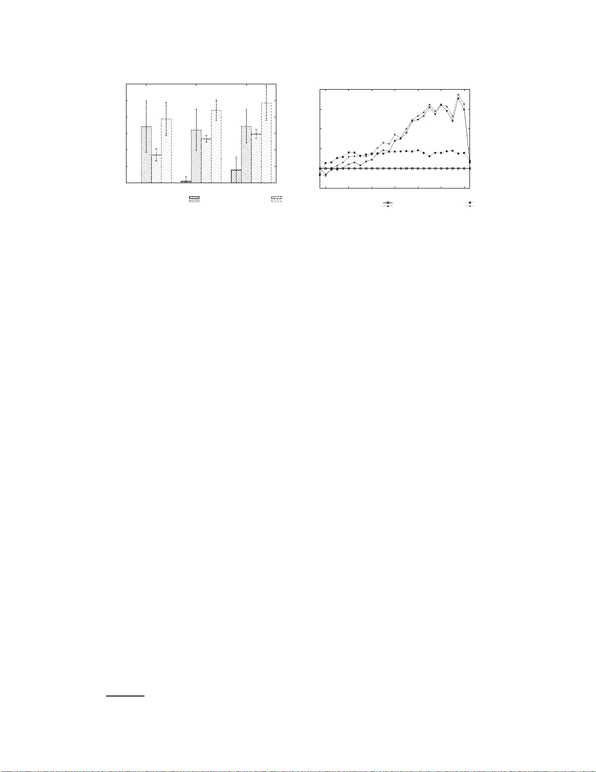
Sequentia l Monte Carlo Inference of Mixed Membership Stochastic Blockmo dels f or Dynamic Social Networks T omoki Kobayashi, Koji Eguchi Graduate School of System Informatics, K obe University 1–1 Rokkodaicho, Nada, K obe 657–8 501, J ap an kobayashi@cs 25.scitec.k obe-u.ac.jp eguchi@port. kobe-u.ac.j p Abstract Many kinds of data can be represented as a network or graph. It is crucial to infer the latent structure underly ing such a network and to predict unobserved link s in the network . Mixed Membership Sto chastic Blockm odel (MMSB) is a promis- ing mod el for network data. Latent variables and u nknown parameters in MMSB have been estimated thro ugh Bayesian inference with the entire network; how- ev er, it is imp ortant to estimate them on line for ev olvin g networks. In this paper, we first dev elop online in ference methods for MMSB through sequential Mo nte Carlo methods, also known as particle filters. W e then extend them f or time- ev olving networks, taking into account the tem poral depend ency o f th e network structure. W e demonstrate thr ough experiments that the time-depen dent particle filter outper formed sev er al baselines in terms of prediction performan ce in an on- line condition. 1 Intr oduction Many p roblem s can be repr esented as network s or grap hs, and deman ds for an alyzing such data have increased in recent years. Specifically , it is cr ucial to infer the latent structure u nderlyin g such a network an d to predict un observed links in the network. One pro mising appro ach to such pro blems is latent variable network mode ling [6]. The latent variable network models can be mainly categorized into tw o kinds. One is hard clustering approach es, su ch as Stochastic Block Models (SBM) [12] and its variants, which assume ea ch no de is assigned to a single cluster or gro up. On the basis of th is assumption, the p robab ility of gener ating a link f rom every node in one cluster to anoth er cluster is always the same. In an extension of SBM, In finite Relational Model (IRM) [9] assumes the infinite number o f clu sters. Th e oth er is soft clu stering app roache s, such as Mixed Memb ership Stoch astic Blockmode ls (MMSB) [1]. MMSB assumes th at each nod e is represented as a mixture o f m ultiple latent groups, and that e very link i s gener ated in accordanc e with a Bernoulli distribution associated with each pair of latent groups. MMSB has been successfully applied as social network analysis and protein- protein interaction prediction [1]. Latent variables and un known parameters in MMSB hav e been estimated by variational Bay esian inference o r collap sed Gibbs sampling with the entire network. Those ar e called batch infer ence algorithm s, requiring sig nificant com putation al time. Howe ver , it is imp ortant to estimate them online f or ev olvin g networks. In the scenar io where n odes or links ar e sequen tially observed over time, it is n ot realistic to u se a batch infer ence algorithm e very time a node or a link is o bserved, so an online inference algorithm is more approp riate in this case. 1 Figure 1: Graphical model of MMSB. Algorithm: batch Gibbs sampler for N × N 1: initialize group assignment randomly for N × N 2: for iteration=1 to S do 3: for p =1 to N do 4: for q =1 to N do 5: draw z p → q from P ( z p → q | Y , Z ¬ ( p,q ) → , Z ¬ ( p,q ) ← , α , ψ ) 6: draw z p ← q from P ( z p ← q | Y , Z ¬ ( p,q ) → , Z ¬ ( p,q ) ← , α , ψ ) 7: end for 8: end for 9: end for 10: complete the posterior estimates of π a nd B Figure 2: Pseudo c odes o f batch Gibbs sam- pler . For topic mod els [3] with text data, various prior studies hav e explored online inf erence [ 2, 4, 8 ]. Howe ver , o nline inference for latent v ariab le n etwork models has not b een explored , to the best of our knowledge. In this pape r , we propo se online inference algorithms fo r MMSB: inc remental Gibbs samp ling meth od and particle filter . Furthermore, we prop ose another o nline in ference al- gorithm that d ynamically adapts the changes in stru cture within a network, in the fram ew or k of a particle filter . W e demonstra te through exper iments that th ese inference me thods work effecti vely for evolving netw or ks. The contributions of this pap er are (1) onlin e inferen ce methods for MMSB and (2) novel o nline inference methods that take into account time depend ency in latent s tru cture of ev olving networks. 2 Mixed Membership Stochastic Blockmodels The Mixed Memb ership Sto chastic Blockmodel (MMSB) w as proposed by Airoldi et al. This mod el assumes that each node is represented as a mixture of latent groups, and that every link is generated in accordanc e with a Bernoulli distribution associated with each pair of latent groups. At first, we summar ize the d efinitions used in th is paper . W e repr esent a simple d irected g raph as G = ( N , Y ) , where ( p, q ) elemen t in an adjacency matrix Y ind icates whether a link (or an arc) is p resent or absent fr om no de (or vertex) p to n ode q as Y ( p, q ) ∈ { 0 , 1 } . Eac h nod e is associated with a multinomial distribution over laten t groups, Mult ( π p ) . Here , π p,g represents the prob ability that n ode p belong s to grou p g . T herefo re, a single node can be assigned with a different group for each co nnected link from that node. Su pposing th at the number o f gr oups is K , the relationship between any pair of gro ups ( g , h ) is repr esented as a Bernoulli distribution, Bern ( B K × K ) . The element B ( g , h ) ind icates the Bernoulli parameter cor respond ing to gro up pair ( g , h ) , rep resenting the pro bability that a link is present between a node in gro up g and an other node in gro up h . Given a link from nod e p to q , the indicator vector z p → q indicates a latent gro up assigned to node p , an d z p ← q indicates a latent group assigned to node q . T hese laten t group indicator vectors are den oted by Z → = { z p → q | p, q ∈ N } and Z ← = { z p ← q | p, q ∈ N } . In accordance with the above definitions, the generative process of MMSB can be described as follows. 1. For each nod e p : • Dr aw a K d imensional vector of multinomial parameters, π p ∼ Dir ( α ) 2. For each pair of grou ps ( g, h ) : • Dr aw a Bernou lli parameter, B ( g , h ) ∼ Beta ( ψ ) 3. For each pair of nodes ( p, q ) • Dr aw an indicator v ecto r for the initiator’ s group assignmen t, z p → q ∼ Mu lt ( π p ) • Dr aw an indicator v ecto r for the recei ver’ s group ass ign ment, z p ← q ∼ Mu lt ( π q ) • Sam ple a binary value that represen ts the p resence o r absen ce of a link, Y ( p, q ) ∼ Bern ( z T p → q Bz p ← q ) 2 A g raphical model representation of MMSB is shown in Fig. 1. The full joint distrib u tion of observed data Y a nd latent variables π 1: N , Z → , Z ← , and B are gi ven as follows: P ( Y , π 1: N , Z → , Z ← , B | α , ψ ) = P ( B | ψ ) Y p,q,p 6 = q P ( Y ( p, q ) | z p → q , z p ← q , B ) P ( z p → q | π p ) P ( z p ← q | π q ) Y p P ( π p | α ) (1) Collapsed Gib bs sampling can estimate latent variables and unkn own param eters of MMSB. The algorithm is outlined in Fig. 2, wh ere it is con verged to posterior distributions. Hereinafter, th is inference alg orithm is refer red to as ba tch Gibbs sample r . This is similar to a collapsed Gibb s sampler for estimating LD A (Latent Dirichlet allocation) for text data [3, 7]. 3 Online Infer ence Algorithms for MMS B This section d escribes how to achieve online infere nce for MMSB, especially b y using the incr e- mental Gibbs sampler and particle filter that were originally dev elop ed for te xt data [2, 4]. 3.1 Incremental Gibb s Sampler Canini at al. [4] de velope d an incremen tal Gibbs sampler, by modify ing batch Gibbs sampler —also known as collap sed Gib bs sampler [7]—, f or estimating an LDA mode l fo r text data in an o nline setting. W e fur ther modify it for MMSB for network data in an on line setting. Giv en a discrete tim e series of network data, we first apply the batch Gibbs sampler to the fir st period of the data. Then , ev ery time the presence or absence of a link is ob served, we run the following steps: 1. Wh en a new link with a old node is observed, we sample a pair of group s in accordance with the full conditiona l probability with already observed data and their group assignments. 2. Wh en a new link with a new node is observed, we sample a pair of groups for ev ery pair of a new node and an already observed node. 3. W e update the latent gr oups for the rejuvenation sequence R ( p, q ) —i.e., |R ( p, q ) | of ran- domly selected n ode pairs that were already observed at the time when nod e pair ( p, q ) is observed—. This step is called r ejuv enation , such as in the literature on particle filters [5]. The larger the |R ( p, q ) | , the more accur ately p osterior distributions c an be estimated. Ho w- ev er, inference time in creases qua dratically with |R ( p, q ) | . If we skip the step of reju venation o r |R ( p, q ) | = 0 , it is similar to the online inferen ce meth od th at Banerjee et al. developed for LD A [ 2]. 3.2 Particle Filter The par ticle filter is also known as a seq uential Monte Carlo method [5]. The infer ence is achieved by the weighted average of multiple particles, e ach of wh ich estimates latent gro up assign ments for o bserved node pairs differently at the same time. Here, th e estimation with each particle is perfor med b y following the three s tep s in an incremental Gibbs sampler , as described in Section 3.1. The weight of each pa rticle is assumed to be propor tional to the likelihood of gen erating observed links by the p article. When the variance of the weight is larger than a thresho ld —referred to as the effecti ve sample size (ESS) thre shold—, resamp ling is p erform ed to create a new set of particles. W e employed a simple resamp ling scheme that dr aws particles fro m the multinomial distribution specified by the normalized weights. After the resampling , the weights are then reset to P − 1 , where P indicates the number of particles. The a lgorithm of the pa rticle filter is outlined in Fig. 3. Note that, in this figure, lines from 5 to 1 8 correspo nd to the n ew link grou p assignment steps in an incremental Gibbs sampler, and lines from 26 to 29 correspo nd to t h e rejuvenation step in an inc remental Gibbs sampler . The posterior distribution of particle fi lter, P particle is represented as follows: P particle = X k P ( k ) × ω ( k ) (2) 3 Algorithm: particle filter 1: initialize weights ω ( k ) = P − 1 for k = 1 , · · · , P 2: while(add link p ′ → q ′ ) 3: for k = 1 t o P do 4: ω ( k ) ∗ = P ( k ) ( Y ( p ′ , q ′ ) = 1 | Y , Z ¬ ( p ′ ,q ′ ) → , Z ¬ ( p ′ ,q ′ ) ← , α , ψ ) 5: draw z ( k ) p ′ → q ′ from P ( k ) ( z p ′ → q ′ | Y , Z ¬ ( p ′ ,q ′ ) → , Z ¬ ( p ′ ,q ′ ) ← , α , ψ ) 6: draw z ( k ) p ′ ← q ′ from P ( k ) ( z p ′ ← q ′ | Y , Z ¬ ( p ′ ,q ′ ) → , Z ¬ ( p ′ ,q ′ ) ← , α , ψ ) 7: if( p ′ is new no de) 8: for q = 1 to N cur r ent (if q 6 = q ′ ) 9: draw z ( k ) p ′ → q from P ( k ) ( z p ′ → q | Y , Z ¬ ( p ′ ,q ) → , Z ¬ ( p ′ ,q ) ← , α , ψ ) 10: draw z ( k ) p ′ ← q from P ( k ) ( z p ′ ← q | Y , Z ¬ ( p ′ ,q ) → , Z ¬ ( p ′ ,q ) ← , α , ψ ) 11: end for 12: end if 13: if( q ′ is new no de) 14: for p = 1 t o N cur r ent (if p 6 = p ′ ) do 15: draw z ( k ) p → q ′ from P ( k ) ( z p → q ′ | Y , Z ¬ ( p,q ′ ) → , Z ¬ ( p,q ′ ) ← , α , ψ ) 16: draw z ( k ) p ← q ′ from P ( k ) ( z p ← q ′ | Y , Z ¬ ( p,q ′ ) → , Z ¬ ( p,q ′ ) ← , α , ψ ) 17: end for 18: end if 19: end for 20: normalize weights ω to sum to 1 21: if k ω k − 2 ≤ ESS threshold then 22: resample particles 23: ω ( k ) = P − 1 for k = 1 , · · · , P 24: end if 25: for k = 1 to P do 26: for( p ′′ → q ′′ in R ( p ′ , q ′ ) ) do 27: draw z ( k ) p ′′ → q ′′ from P ( k ) ( z p ′′ → q ′′ | Y , Z ¬ ( p ′′ ,q ′′ ) → , Z ¬ ( p ′′ ,q ′′ ) ← , α , ψ ) 28: draw z ( k ) p ′′ ← q ′′ from P ( k ) ( z p ′′ ← q ′′ | Y , Z ¬ ( p ′′ ,q ′′ ) → , Z ¬ ( p ′′ ,q ′′ ) ← , α , ψ ) 29: end for 30: end for 31: end while 32: complete the posterior estimates of π and B Figure 3: Pseudo co des of particle filter . where P ( k ) indicates the p osterior distribution of particle k . ω ( k ) indicates the weight of particle k , which is propo rtional to the likelihood of generating observed links by the particle. 4 T ime-dependent Algorithms W e have in troduc ed the inference method s for MMSB, which estimate the laten t variables and un- known parameter s with already observed data, assuming the network data are sequentially observed over time. Howev er, using all the observed d ata does not a lways resu lt in a ccurate estimation. For instance, you r movie preferences, which ca n be expressed by a bip artite grap h, may sometimes change over time. As ano ther example, en terprise email comm unication s expressed as a n etwork may be c hanged in a structur e when serio us inciden ts happen in th at co mpany . In such ca ses, mor e accurate estimation can be achieved by only considering recent observations and disregard ing older observations. On the basis of the id ea mentioned above, we propo se a time-dependent particle filter for MMSB to capture changes in network structure over time. W e now describe th e method mor e f ormally an d in more detail. Suppose that L t represents the likelihood of observations at time t . W e partially disregard the past observations wh en the following condition is satisfied. λ t = L t L t − 1 < λ 0 (3) where λ t indicates the change rate on the likelihood of observations at time interval t , and λ 0 indi- cates a threshold parameter . W e assume that the pattern of observations is changed when the change 4 rate is small. When Eq. (3) is satisfied, we further compute Λ i,t = ( λ i +1 , . . . , λ t − 1 , λ t ) , where each compon ent indicates the change rate of likelihood of observations for each time interval from i to t , respectively . Here , i is the first time interval that the model consider s, so when an y time interval was discarded previously , i = 1 . W e then sample a time interval to be discarded from a multinomial dis- tribution, whose multinomial parameters are estimated in accord ance with Λ i,t . When time interval τ ( i ≤ τ < t ) is sampled , all the time intervals from i to τ are then discard ed. Once the time interval to be disregarded τ is sampled, we run the following proce dure: • When a nod e is adjacent to any observed n ode a t time interval τ , set the correspo nding element of adjacency matrix to be 0. • Rand omly assign a latent group to each of these node pairs. • When a node is not adjacent to any observed node at time interval τ , assume the node to be unobserved . W e can ap ply this algorithm to the increm ental Gibbs samp ler and particle filter . When we apply it to the particle filter , we compute Λ i,t for each particle. Therefor e, each particle can make a different decision on whether or n ot the past observations should be disregard and which time intervals should be discarded. 5 Experiments In this sectio n, we explore the pre diction perfor mance o f MMSB estimated via online inf erence algorithm s. For e xp eriments, we use time-series network data. 5.1 Settings 5.1.1 Data For experiments, we use a da taset from the Enro n email communication ar chive [10]. The time period of the d ataset is 28 mo nths, fr om Decem ber 1999 to March 2002. This dataset is the same as that used b y T ang et al. [13], whe re emails in certain folde rs were removed from each user f or the use of email classification researc h. This dataset was furth er cleaned so that o nly the users ( i.e., email add resses) who send and receive at least fi ve emails are inclu ded. W e o nly use the relations between users —we assum e a link fro m a user to another wh en a user send s at least one email to another—, disregarding the text content of email messages. This dataset contains 235 6 nodes. W e d ivide a set o f observations (each lin k of which is observed to be pre sent or absent for a p air of no des) evenly into five sets, for the use of five-fold cr oss validation. W e fur ther divide each set into a test set and a validation set, and the remain ing four sets are u sed as training set. W e b riefly summarize the training set, validation s et, a nd test set: T r aining set W e use the n ode p airs included in the training set to estimate the mode l. T he ob - servations (ea ch link of wh ich is ob served to be present or absent f or a pair of nodes) are sequentially added over time. V alidation set W e use the node pairs i n cluded in the v alidation s et to determine ESS threshold and λ 0 threshold for particle filters. T est set W e use th e test set to ev alu ate the inference algorithms. W e co mpute the likelihood of the data within the test set at tim e in terval t using the m odel estimated with th e observations within the training set until time ( t − 1) . 5.1.2 Inference methods In the experiments, we compare the following algorithms. Batch Gibbs sampler For comparison with onlin e inference, we apply the batch Gibbs sampler by varying the numb er of Gibbs sweeps (iterations) as S ∈ { 50 , 100 , 150 , 20 0 , 250 } . 5 0 0.005 0.01 0.015 0.02 0.025 0 100000 200000 300000 400000 500000 600000 rate of increase time to estimate the models (s) batch Gibbs sampler incremental Gibbs sampler 0 0.005 0.01 0.015 0.02 0.025 0 100000 200000 300000 400000 500000 600000 rate of increase time to estimate the models (s) batch Gibbs sampler incremental Gibbs sampler Figure 4: Comparison of batch Gibbs sampler an d incrementa l Gibbs sampler . E rror bars r epresent one sample standard deviation. Incremental Gibb s sampler In the experiment to compare the batch Gibbs sampler , we set the size of re juvenation sequence |R ( p, q ) | ∈ { 0 , 1 K , 5 K , 10 K , 20 K , 30 K , 40 K } . In the oth er experiments, we set |R ( p, q ) | ∈ { 0 , 10 , 10 0 } . For all the o nline algorith ms, we carried out the batch Gibbs sampling fo r the first time interval, setting the num ber of Gibbs sweep s (iterations) to be S = 10 0 . Particle filter W e p erform ed a grid search for ESS thre shold over { 4 , 8 , 12 , 16 , 20 } for each |R ( p, q ) | setting . W e fix th e number of par ticles to 24 in all the con ditions. Using the validation s et, we d etermine ESS threshold for each |R ( p, q ) | settin g. Time-dependent in cremental Gibbs sampler For compa rison, we cond ucted the experiments with th e in cremental Gibb s samp ler in the same manner as the tim e-depen dent particle filter . Time-dependent particle filter W e expe riment with λ 0 threshold in Eq. ( 3) as 1.0, 1.1, 1.2, 1.3, and 1. 4 for each |R ( p, q ) | setting. Using the validation set, we d etermine the op timal λ 0 for each |R ( p, q ) | setting. 5.1.3 Evaluation metrics Suppose that T = { 1 , · · · , T } represents discrete time interv als for a target n etwork. W e then finally ev aluate the p rediction perform ance of each mode l usin g the sum of r ate of increase in ter ms of test-set log-likelihood : 1 T T X t =1 X ( t ) − I 0 ( t ) | I 0 ( t ) | (4) where I 0 ( t ) r epresents test-set log -likelihood with the b aseline: increm ental Gibbs sampler at time interval t whe n |R ( p, q ) | = 0 . X ( t ) r epresents test-set log-likelihoo d with the target inference method at time interval t . According to the definition of the prediction performan ce metric given by Eq. (4), the prediction p erform ance of incr emental Gibb s sampler is zer o wh en |R ( p, q ) | = 0 . The greater the value of Eq. (4), the more effecti vely the model works compared with the baseline. 5.2 Results 5.2.1 Batch vs. online inference T o unde rstand how online inferen ce methods work, we compare an incremental Gibbs samp ler and batch Gibbs sampler, using one of the five sets that were co nstructed f or fiv e-f old cro ss validation. W e experimen ted with a machine with a 48-gig abyte memory and a 12 -core (2 4-thread ) CPU of 3.06GHz clock speed. The results are shown in Fig. 4, where the times (in seconds) to estimate each model an d rate of increase of pred iction perfo rmance in terms of Eq . (4) ar e de monstrated. In the case of batch Gibbs sampler, the plots fr om the left to the r ight represent S = 50 , 100 , 1 50 , 20 0 , and 250 , respectively , indicatin g that the larger the Gibbs sweep s employed, the longer the required estimation time but the better the pred iction p erform ance. I n the case o f an incr emental Gibbs 6 0 0.002 0.004 0.006 0.008 0.01 0.012 0 10 100 rate of increase |R(p,q)| incremental Gibbs incremental Gibbs(Time-dependent) particle Filter particle Filter(Time-dependent) 0 0.002 0.004 0.006 0.008 0.01 0.012 0 10 100 rate of increase |R(p,q)| incremental Gibbs incremental Gibbs(Time-dependent) particle Filter particle Filter(Time-dependent) Figure 5: Prediction pe rforma nce o f time- depend ent infer ence methods. Erro r b ars repr e- sent one sample standard deviation. -0.005 0 0.005 0.01 0.015 0.02 Jan. 2000 May 2000 Sep 2000 Jan. 2001 May 2000 Sep 2000 Jan. 2002 rate of increase time stamp incremental Gibbs incremental Gibbs(Time-dependent) particle Filter particle Filter(Time-dependent) -0.005 0 0.005 0.01 0.015 0.02 Jan. 2000 May 2000 Sep 2000 Jan. 2001 May 2000 Sep 2000 Jan. 2002 rate of increase time stamp incremental Gibbs incremental Gibbs(Time-dependent) particle Filter particle Filter(Time-dependent) Figure 6: Pred iction perfo rmance of time- depend ent inferen ce metho ds in t ime series plots. sampler, the plots fr om the left to th e r ight rep resent |R ( p, q ) | = 0 , 1 K , 5 K , 10 K , 2 0 K , 30 K , and 40 K , re spectiv ely , indicating that the larger the assumed reju venation sequence , the longer the required estimation time but the better the prediction performance. As you can see in Fig. 4, online inference with an in cremental Gibbs sampler is much faster than that with a ba tch Gibbs sampler . Both inferen ce metho ds are almost conv erged at around 0.018 of predic - tion perfor mance. T o achie ve that prediction perfo rmance, the batch Gibbs sampler (when S = 2 00 ) took 475,3 74 secon ds o n average, while the incremental Gibbs sampler (when |R ( p, q ) | = 10 K ) took 151,027 seconds on a verage: 32% of that of the batch Gibbs sampler . Anoth er online inferen ce method, the particle filter, b ehaves similarly to ( thoug h slightly d ifferently from) the increme ntal Gibbs sampler but very differently from the batch Gibbs sampler . Moreover , the batch Gibbs sampler is inv oked at e very time interval, so it takes more time when we assume finer time intervals. On the o ther hand, on line infer ence meth ods such as the in cremental Gibbs sampler an d particle filter take co nstant time since we update the latent variables and unknown parameters sequentially , no matter ho w we define time intervals. For these reasons, online inference is more appropr iate for when the target network is sequentially observed. 5.2.2 Incremental Gib bs sampler vs. partic le filter Fig. 5 shows the prediction perform ance of the incr emental Gibbs sampler and particle filter using time-indep endent and time-d epend ent a lgorithms, respectiv ely . T he ru n time of th e particle filter is six times longer tha n th at o f incremental Gibbs for the same |R ( p, q ) | setting; howe ver , it is much less than that o f the batch Gibbs sampler . The g reater the |R ( p, q ) | , the better the prediction perfor mance but the longe r the require d tim e. As shown in Fig. 5, the predictio n perf ormanc e of particle filter is greater than that of incremen tal Gibbs in any |R ( p, q ) | setting. 5.2.3 Time-dependent algo rithms f or incremental Gibbs s ampler a nd particle filter As shown in Fig. 5, th e time-depen dent algo rithm works e ffecti vely in b oth the incr emental Gibbs sampler and par ticle filter . More over , the prediction perf ormanc e of the tim e-depen dent p article filter is greater than that of the time-depen dent increme ntal Gibbs sampler . The Enron Cor poration —an U.S. energy , co mmodities, and serv ices company— experience d a drop in stock market price from around January 2 001 and th en declared bankruptcy on December 2, 2001. The datasets we used for experiments are based on email communic ations within that company from December 1999 to March 20 02, as we mention ed pr eviously . Th erefore, the network structur e of email communication s should be continuou sly changed, especially from January 2001 to December 2001. W e dem onstrate whether and how effecti vely the time-depend ent infe rence metho ds cap- ture the ch ange in Fig. 6, by plottin g in time order the improvements in prediction performan ce, X ( t ) − I 0 ( t ) | I 0 ( t ) | in Eq.(4), on th e basis o f tha t of the incremen tal Gibbs sampler when |R ( p, q ) | = 0 . As you can see in this figu re, the time-dep endent par ticle filter and time-dep endent incre mental Gibbs 7 sampler o utperfo rm the time-indepen dent m ethods, especially from January 2001 . Th is indicates that the tim e-depen dent inf erence methods adequately captur e the chang e in structure of th e email commun ications durin g the crisis at the company , by removing p ast observations in online inference. 6 Conclusions In this pape r , w e proposed online inference methods for Mixed Member ship Stochastic Blockmodels (MMSB) that ha ve ne ver been explored . Furthermo re, we also proposed ti me -depen dent algorithm s for the on line in ference of MMSB, reflecting the change in stru cture of the network d ata over time by selectiv ely discar ding the past o bservations when th e chang e oc curs. W e experim ented with an email comm unication dataset to evaluate both the p rediction perfor mance and the time required for the estimation. W e demonstrated that p article filter im proved pr ediction performance c ompared with the baselines of the batch Gibbs sampler and incremental Gibbs sampler . W e also demonstrated that the time-depen dent particle filter works more ef fectively than either the naive particle filter or time- depend ent incremen tal Gibbs sampler . More detailed e valuation is left for our future work. Applyin g our inferen ce methods to a nonpar ametric relational mod el [11] is one of the possible dir ections for the future work. Acknowledgments: This work was supp orted in part b y the Grant-in-Aid fo r Scientific Research (#233 0003 9) from JSPS, Japan. Refer ences [1] E. M. Air oldi, D. M. Blei, S. E . Fien berg, and E. P . Xin g. Mixed m embership stochastic blockmo dels. Journal of Machine Learning Researc h , 9:1981 –201 4, 2008. [2] A. Banerjee an d S. Basu. T opic models over text stream s: A study of batch and onlin e un su- pervised learnin g. In Pr oceed ings of the 7th SI AM Interna tional Confer ence o n Data Min ing , pages 437– 442, Minneapolis, Minnesota, USA, 200 7. [3] D. M. Blei, A. Y . Ng, and M. I. Jo rdan. Latent Dirichlet allocatio n. J ou rnal of Machine Learning Resear ch , 3:993–10 22, 2003. [4] K. R. Canini, L. Shi, and T . L. Griffiths. Online inf erence of to pics with latent Dirichlet allocation. In Pr oc eedings o f th e 1 2th I nternation al Confer ence o n A rtificial I ntelligence and Statistics , pages 65–72 , Clearwater Beach, Florida, USA, 2009. [5] A. Dou cet, N. De Freitas, N. Gor don, et al. S equentia l Monte Carlo Method s in Practice . Springer New Y ork, 2001. [6] A. Goldenberg, A . X. Zheng, S. E. Fienberg, and E. M. Airoldi. A s ur vey of statistical network models. F o unda tions and T rends in Machine Learning , 2(2):129–2 33, 2010. [7] T . L. Griffiths a nd M. Ste yvers. Finding scientific topics. Pr o ceedings of the National Academy of Sciences of the United States of America , 101:522 8–52 35, 2 004. [8] M. Hoffman, F . R. Bach, an d D. M. Blei. O nline learning f or latent Dir ichlet allo cation. In Advance s i n Neural Information Pr ocessing Systems , volume 23, pages 856–864, 2010. [9] C. Kemp, J. B. T enenbau m, T . L. Griffiths, T . Y amad a, and N. Ued a. Learning systems of concepts with an infinite relational model. In Pr o ceedings of the 21 st National Conference on Artificial Intelligence , v olum e 1, pages 381–388, Boston, Massachusetts, USA, 2006. [10] B. Klimt an d Y . Y ang. Intr oducing the En ron corp us. In F irst Co nfer ence o n Email a nd An ti- Spam CEAS , Mountain V iew , California, USA, 2004. [11] K. Miller, M. I. Jordan, and T . L. Gr iffiths. Nonp arametric latent f eature m odels for link prediction . In Adva nces in Neural Information Pr ocessing S ystems , volume 22, pages 1276 – 1284, 2009. [12] K. Nowicki and T . A. B. Sn ijders. Estimation a nd pred iction for stochastic b lockstructu res. Journal of the American Statistical Association , 96(455):1 077– 1087, 200 1. [13] L . T ang , H. Liu, J. Zhang, and Z . Nazeri. Community ev olutio n in dynam ic multi-mo de n et- works. In Pr oceedin gs o f the 14th AC M SIGKDD Intern ational Confer ence on Knowledge Discovery and Data Mining , pages 677–68 5, Las V egas, Ne vada, USA, 2008. 8