From Maxout to Channel-Out: Encoding Information on Sparse Pathways

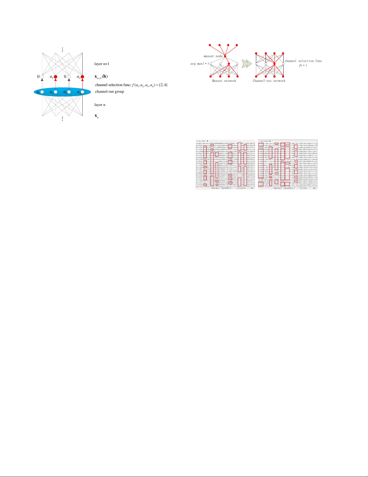
Fr om Maxout to Channel-Out: Encoding Inf ormation on Sparse Pathways Qi W ang Department of ECE and Institute for Adv anced Computer Studies Uni versity of Maryland College P ark, MD qwang37@umiacs.umd.edu Joseph JaJa Department of ECE and Institute for Adv anced Computer Studies Uni versity of Maryland College P ark, MD joseph@umiacs.umd.edu Abstract Motivated by an important insight fr om neural science, we pr opose a ne w frame work for understanding the success of the r ecently pr oposed “maxout” networks. The frame- work is based on encoding information on sparse path- ways and r ecognizing the corr ect pathway at infer ence time. Elaborating further on this insight, we pr opose a novel deep network arc hitectur e, called “channel-out” network, which takes a much better advantage of sparse pathway encoding. In channel-out networks, pathways are not only formed a posteriori, but the y ar e also actively selected accor ding to the infer ence outputs from the lower layers. F r om a math- ematical perspective, channel-out networks can repr esent a wider class of piece-wise continuous functions, ther eby en- dowing the network with mor e expr essive power than that of maxout networks. W e test our channel-out networks on sever al well-known image classification benc hmarks, set- ting new state-of-the-art performance on CIF AR-100 and STL-10, which repr esent some of the “har der” image clas- sification benchmarks. 1. Introduction Most of the recent work on deep learning has focused on ways to re gularize network behavior to a void over -fitting. Dropout [8] has been widely accepted as an effecti ve way for deep network regularization. Dropout was initially pro- posed to avoid co-adaptation of feature detectors, but it turns out it can also be re garded as an efficient ensemble model. The maxout network [7] is a newly proposed micro architecture of deep networks, which works well with the dropout technique. It sets the state-of-the-art performance on many popular image classification datasets. In retro- spect, both methods follow the same approach: they restrict updates triggered by a training sample to affect only a sparse sub-graph of the network. W e note that neural science re- searchers ha ve come up with what can be percei ved as a similar principle from years of study of the human brain: It is not the shape of the signal, but the pathway along which the signal flows, that determines the functionality [10]. W e use this principle as an important clue to explore the encod- ing capabilities of deep networks. In this paper we provide a ne w insight into a possible reason for the success of maxout, namely that it partially takes advantage of what we call “sparse pathway coding”, a much more robust way of encoding categorical information than encoding by magnitudes. In sparse pathway encoding, the pathway selection itself carries significant amount of the categorical information. W ith a carefully designed scheme, the netw ork can extract pattern-specific pathways during training time and recognize the correct pathway at inference time. Guided by this principle, we propose a new class of network architectures called “channel-out networks”. Un- like the maxout netw ork, this type of networks does not only form sparse input pathways a posteriori, but it also activ ely selects outgoing pathways. W e run experiments on channel-out networks using sev eral image classification benchmarks, all of which show similar or better perfor- mance results compared with maxout. In fact, the channel- out network sets new state-of-the-art performance on some image classification datasets that are on the “harder” end of the spectrum (i.e., those with lower current state-of-the- art performance), namely CIF AR-100 and STL-10, demon- strating its potential to encode large amounts of informa- tion with higher lev el of complexity . Channel-out is just one example of using the sparse pathway encoding princi- ple, which we belie ve is a promising research direction for designing other types of deep network architectures. 2. Dr opout vs Maxout: Ensemble of Sub- Models vs Recognizable Sub-Models In this section we briefly revie w the concepts of dropout [8] and maxout [7], and introduce the concept of sparse 1 pathway encoding. Dropout regularizes the network during the training phase by randomly crossing out some of the nodes upon the processing of each training sample. Therefore it restricts the updates to happen only along a relati vely sparse sub- network. As has been pointed out in a number of papers [8, 18, 20], dropout networks can be regarded as perform- ing efficient model av eraging of a large ensemble of models randomly sampled from the original network, so that each model learns a different representation of the data. The maxout network is a recently proposed micro- architecture that is significantly different from traditional networks: the activ ation function does not take a normal single-input-single-output form, but instead the maximum of the activ ations from sev eral candidate nodes. In [7], the advantage of maxout over normal differentiable acti- vation functions (such as tanh) was attributed to its better approximation to the exact model av eraging, and the ad- vantage of maxout ov er the rectified linear activ ation func- tion was attrib uted to easier optimization on maxout net- works. Here we propose another insight of the po wer of the maxout network. The maxout node acti vates only one of the candidate input pathways depending on the input, and when the gradient (the novel information discov ered from the current training sample) is back-propagated, only that selected pathway is updated with the information, which it encodes (Figure 1). Therefore the information con veyed by each training sample is compactly encoded onto a local por- tion of the network, instead of being disseminated across the entire network. W e call this behavior as “sparse path- way coding”. Moreover , due to the local in variance of the max-linear function, the network can “remember” the cor- rect pathway selection for the same or similar test sample. At inference time, if a test sample is similar to a certain pattern encoded, then it is more likely to activ ate a path- way that is similar to the one activ ated by this pattern. Cor- rect inference can therefore be made with awareness of that pattern-specific pathway . T o sum up, The maxout network encodes information sparsely on distinct pathways, and has the capability of re- trieving the correct pathway at inference time. This obser- vation is well in line with the f amous principle in neural science, “The information con veyed by an action potential is determined not by the form of the signal but by the path- way the signal trav els in the brain” [10]. 3. Channel-Out Networks 3.1. Pushing the sparse pathway concept further Although maxout networks implement the concept of sparse pathway coding, the pathways are formed “a pos- teriori”, meaning that a pathway selection is only implicitly implemented with already-formed input paths, but no activ e max(·) max-out node winner Figure 1: Sparse pathway coding by maxout networks. Ef- fectiv e information flows only along the red links. link selection is e ver made. Higher layer pathway selections are not aware of the selections made in lower layers. A nat- ural extension is to endow the network with the capability of active output pathway selection, which may result in a more efficient pathway coding. Along this line, we propose a class of new deep network architectures called “channel- out networks”. A channel-out netw ork is characterized by channel-out groups (Figure 2). At the end of the linear portion in a typical layer (can be fully connected, con volutional, or lo- cally connected), output nodes are arranged into groups, and for each group, a special channel selection function is performed to decide which channel opens for further in- formation flo w . Only the activ ation of the selected chan- nel is passed through, all other channels are blocked off (this is realized by ma sking the corresponding channel out- put by 0). When the gradient is back-propagated through this channel-out layer , it only passes through the open channels selected during forward propagation. F ormally , we first define a vector -valued channel selection function f ( a 1 , a 2 , ..., a k ) which takes as input a vector of length k and outputs an index set of length l ( l < k ). Elements of the index set are selected from the domain { 1 , 2 , ..., k } . Then with an input vector (typically the pre vious layer output) a = ( a 1 , a 2 , ..., a k ) ∈ R k , a channel-out group implements the following activ ation functions: h i = I { i ∈ f ( a 1 ,a 2 ,...,a k ) } a i (1) where I ( · ) is the indicator function, i indexes the candidates in the channel-out group, a i is the i th candidate input, and h i is the output (Figure 2). There are many possible choices of the channel selection function f ( · ) . T o ensure good per- formance, we require that the channel selection function possesses the following properties: • The function must be piece-wise constant, and the piece-wise constant regions should not be too small. Intuitiv ely , the function has to be “regular enough” to ensure robustness against the noise in the data. 2 1 2 3 4 c h a n n e l s e l e c t i o n f u n c : ( , , , ) { 2 , 4 } f a a a a  1 a 2 a 3 a 4 a 0 2 a 0 4 a n x 1 ( ) n  x h ... ... layer n layer n+1 channel-out gr oup Figure 2: Operation performed by a channel-out group • The pre-image size of each possible index output must be of almost the same size. In other words, each chan- nel in the channel-out group should be equally likely to be selected as we process the training examples (so that the information capacity of the network is fully utilized). • The computation cost for ev aluating the function must be as low as possible. Some examples of good channel selection functions are: arg max( · ) , arg min( · ) , arg median( · ) , indices of the l largest candidates, and the absolute-max arg max( | · | ) . The test results reported in this paper all used the arg max( · ) function. The characteristics of a channel-out network is better il- lustrated through a com parison with the maxout network (Figure 3). In a maxo ut network, a maxout node only takes the maximum value of the candidates, without the outgoing links being aware of the index. In contrast, in the channel- out network, the channel-out group kno ws about the index of the open channel, and output link selection is made possi- ble by this extra piece of information. In summary , the main characteristic of a channel-out network is that a channel-out group uses channel selection information to determine fu- ture inference pathways. In a deep con volutional network for 2D image classifica- tion, channel-out groups can be implemented by perform- ing the channel selection function across groups of feature maps after con volution/multiplication. Similar to maxout networks, channel-out can be regarded as a special kind of cross-feature pooling. Moreover , in addition to the chan- nel output value, h f ( a ) , the index vector itself f ( a ) should also be recorded into an index matrix, so that the open path- way can be retriev ed during back-propagation. W e can further take advantage of the index vector to implement sparse con volution and sparse matrix multiplication, av oid- ing wasteful computations of multiplications by zeros. This arg max(·) maxout node Maxout network Channel-out network channel selection func f (·) Figure 3: Difference between maxout and channel-out: A maxout node is attached to a set of FIXED output links, resulting in same output pathway for different input path- ways; A channel-out group is connected to a set of different output links, resulting in distinct output pathways. (a) Automobile (b) Frog Figure 4: Pathw ay patterns for two classes in CIF AR-10 can potentially make the computation very fast. T raining a channel-out network that has a similar number of parame- ters as a maxout network, assuming a scalar channel selec- tion function, can in theory be done k times faster than the maxout network, where k is the size of channel-out/maxout groups. W e are currently working on this fast implementa- tion. T o confirm that pathway selection is indeed indicati ve of the patterns in the data, we record the pathway selec- tions of a well-trained maxout model and a channel-out model (with max( · ) channel selection function) using the CIF AR-10 dataset. For ease of visualization and analysis, we set the size of maxout/channel-out groups to 2, so that we can use 0/1 to represent the pathway selection at each maxout/channel-out group. Figure 4 sho ws the channel-out pathway patterns of two classes, where each row records the pathway selections of all channel-out groups (only part of them are sho wn in the window) when performing infer- ence on a specific test sample. W e can clearly observe many class-specific string patterns, indicating that pathway selec- tion patterns indeed subsume important clue of categoriza- tion. Some of the salient patterns have been marked with red rectangles. T o better visualize the space of pathway patterns, we perform PCA analysis on the pathway pattern vectors and project them into the three dimensional space. Figures 5 and 6 sho w the results f or channel-out and maxout, respec- tiv ely . W e can see that clusters have been well formed. 3 −40 −20 0 −30 −20 −10 0 10 20 30 −25 −20 −15 −10 −5 0 5 10 15 20 25 airplane automobile bird cat deer dog frog horse ship truck −30 −20 −10 0 −30 −20 −10 0 10 20 30 −30 −20 −10 0 10 20 30 airplane automobile bird cat deer dog frog horse ship truck Figure 5: 3D visualization of the pathway pattern: channel- out −100 −50 0 −40 −30 −20 −10 0 10 20 30 40 50 −40 −30 −20 −10 0 10 20 30 40 airplane automobile bird cat deer dog frog horse ship truck −55 −50 −45 −40 −35 −30 −25 −20 −15 −40 −20 0 20 40 60 −40 −30 −20 −10 0 10 20 30 40 airplane automobile bird cat deer dog frog horse ship truck Figure 6: 3D visualization of the pathway pattern: maxout Although these clusters are not perfect, they still demon- strate that considerable amount of categorical information has been encoded by pathw ay patterns. W e can also see that the channel-out model results in better clusters than those generated by maxout. For example, the frog class (yellow stars) is better separated from the other classes in the channel-out case. Another interesting observation is that, while the channel-out and maxout models have been trained independently with completely random parameter initialization, the relativ e 3D positions of the classes in the visualization show very similar spatial structures. This im- plies that the pathway pattern provides a very robust repre- sentation of the underlying patterns in the data. In the next few sub-sections we argue from different per- spectiv es why the channel-out network manifests the con- cept of sparse pathw a y selection better than maxout, and why it can potentially exhibit better performances on clas- sification tasks. 3.2. Expressiv e power of the channel-out network Univ ersal representation/approximation property is a good indication of the expressi ve po wer of a model. The fact that a two-layer circuit of logic gates can represent any boolean function [14] implies the nonlinear expressi ve power of early shallo w neural networks. Existence of func- tions that are computable with polynomial-size networks with k layers while requiring exponential-size networks with k − 1 layers implies the benefit of using deep archi- tectures [1]. More recently , the fact that maxout networks are univ ersal approximator of any continuous function is an indication of its good performance [7]. Channel-out net- works also ha ve strong universal approximation properties. T ake the max( · ) channel selection function as an example, we can prov e the follo wing theorem: Theorem: Any piece-wise continuous function defined on a compact domain in Euclidean space can be appr ox- imated arbitrarily well by a max( · ) two-layer c hannel- out network with one hidden channel-out gr oup with fi- nite number of candidate nodes. That is, denote the tar- get function to be approximated as T ( x ) , then ∀ � > 0 , we can find a two-layer channel-out network with one hid- den channel-out gr oup that implements a function F ( · ) such that  | T ( x ) − F ( x ) | 2 dx < � . Her e by a “piece-wise con- tinuous function” we refer to a function that is constituted of finite number of continuous segments. The proof is straightforward and is not of much technical significance. It is listed in the Appendix section. 3.3. Channel-out network does more efficient path- way switching Local learning behaviors on maxout and channel-out net- works can be categorized into two classes: activ ation tuning (mild change) and pa thway switching (critical change). Ac- tiv ation tuning happens when the desired parameter update is not significant enough to change the pathway selection, otherwise pathway switching occurs. Channel-out and max- out networks show very different behaviors upon pathway switching. W e discuss it under a simple scenario in which we repeatedly present the same training sample to the net- work. For a maxout node, when pathway switching hap- pens, the gradient propagated to the maxout node must be to decrease the acti v ation. Howe ver , the ef fective acti va- tion decrease will be thresholded by the acti v ation le vel of the second largest candidate acti vation, which slo ws down, but does not steer aw ay the decreasing trend (we are as- suming that the network structure above this maxout node is relati vely in variant across dif ferent presentations of the training sample). Under this scenario, updates will typically alternate between candidate pathways, reducing the overall efficienc y of updates. In contrast, for a channel-out net- work, whenev er a pathway switches in a channel-out group, the effecti ve structure above the channel-out group is dras- tically changed due to the distinct output links selected by the channel-out group, resulting in significant change in the desired direction of the activ ation update. In other words, when current pathway is too far from fitting the data well, the channel-out group tends to switch and start training a new pathway from scratch. Clearly this is a more desired behavior for pathway switching. 4. Sparse Pathway Selection as a Regulariza- tion Method In this section we consider different principles under- lying sparse pathway methods (channel-out/maxout) and dropout in terms of regularizing network training. W e argue that the strengths of sparse pathway selection and dropout complement each other . This explains the main reason 4 that sparse pathway methods, when combined with dropout, outperforms traditional neural network models. W e belie ve that sparse pathway encoding is a general direction that is well worth pursuing in future research for designing deep network architectures. Maxout and channel-out networks are just two examples along this direction. 4.1. Dropout regularization: squeezing all informa- tion into each sub-network Recall that dropout, with each presentation of a training sample, samples a sub-network and encodes the informa- tion rev ealed by the training sample onto this sub-network. Since the sampling of data and sub-networks are indepen- dent processes, in a statistical sense the information pro- vided by each training sample will ev entually be “squeezed” into all these sub-networks (third row of Figure 7). The adv antage of such scheme, as has been pointed out in various papers [8, 18, 20], is that the same piece of in- formation is encoded into many dif ferent representations, adding to the robustness at inference time. The side-effect, which has not been highlighted before, is that encoding conflicting pieces of information densely into sub-networks with small capacities causes interference problem. Data samples of dif ferent patterns (classes) attempt to build dif- ferent, maybe highly conflicting network representations. When the sub-netw ork is not large enough to hold all the information, conflicting parts tend to cancel each other , re- sulting in significant information loss. An extreme case is the practice of training sev eral networks independently (on the same dataset) and combine them by naiv e av eraging of the link weights, which clearly does not make much sense in general. Note that although dropout is disseminating the training set information over the entire network, it is significantly different from a normal deep network without any regu- larization. For the latt er , retrie val of information relies on ov erall cooperation of the entire network, where each sub- network only encodes P AR T of the information (second ro w of Figure 7). In contrast the dropout network tries to en- code the entire information in EA CH sub-network. Sub- networks interact with each other more by averaging (or voting), rather than by cooperation. 4.2. Sparse pathway regularization: encoding dif- ferent patterns into different sub-networks In contrast to dropout, sparse pathway regularization methods tend to encode information in a more specialized way . Each pattern of the training data is likely to be en- coded onto one or a few specialized sub-networks (for the simplest case, readers can consider each class as of one pat- tern). This is illustrated in the fourth row of Figure 7. Clearly , sparse pathway methods mitigate the interfer- ence problem caused by dropout. The problem with pure Pr o tot y p e s :   Ne twor k  c ap a ci t y:  En c o di ng pa t t er n  o nt r ad i t i on al d e e p n e twor k s Drop out en co di n g  pa t t e r n Ch a nnel - o ut /Max out enc o di ng p a t t e r n Drop out + C h a nnel - o u t /Max ou t enco d i n g pa t t e r n Figure 7: Information encoding patterns. Each bin of the network capacity represents a certain size sub-network. Dropout tends to encode all patterns to each capacity bin, re- sulting in efficient use of network capacity but high level of interference; Sparse pathway methods tend to encode each pattern to a specific sparse sub-netw ork, resulting in least interference but waste of network capacity; The best ap- proach is the combination of the two schemes. sparse path way regularization, howe ver , is that network capacity could be under -utilized. Since sub-networks are highly pattern-specific, and there are only a fe w fundamen- tal patterns in the data, only a small subset of the entire net- work is selected and trained, leaving the rest of the network capacity in an “idle” state. This is a waste of the network capacity . Now it is not hard to understand why combining dropout and sparse pathway encoding could result in bet- ter performance: the combination takes adv antage of the strengths of both methods to do more efficient information coding, as illustrated in the last row of Figure 7. Notice that encoding data pattern(s) into sparse path- ways is also dif ferent from encoding partial patterns into sub-networks, as is done in a normal network without reg- ularization. In a non-regularized network, the information encoded on a sub-netw ork is not likely to form complete patterns, while in sparse pathway methods a certain sub- network always tries to encode complete patterns. Here we note also the significant difference between sparse pathway methods and standard sparse feature learning techniques [3, 13, 16], which is that a sparse pathway model must also possess the ability of RECOGNIZING the correct pathway during inference time. An empirical observation in support of our arguments about dropout/sparse pathway encoding pattern is seen when we take e xtremes of either of the regularization di- rections in our experiments. W e observe that when dropout rate is set too high (number of alive nodes too few for each training sample), the d ominating problem is under-fitting, where we see both training and test set precision cease to 5 improv e at very early epochs. When no dropout is applied, the dominating problem is ov er-fitting, where we see train- ing set precision growing very fast while test set precision is not catching up with the improvement of training set fitness. This is in line with our major assumption about deficiencies of each method: dropout causes interference, while pure sparse pathway encoding forgoes using redundant network capacity to enhance robustness, thus is more vulnerable to ov er-fitting. 5. Benchmark Results 5.1. Overview of results In this section we show the performance of the channel- out network on several image classification benchmarks. For all the channel-out networks used in our experiments, the channel selection function is the max( · ) function. W e run tests on CIF AR-10, CIF AR-100 [11] and STL-10 [4], significantly outperforming the state-of-the-art results on the last two datasets. Our implementation is built on top of the efficient conv o- lution CUDA kernels dev eloped by Alex Krizhevsk y [11]. Most experiments are done using a T esla C2050 GPU. Due to the time limit, we had to control the size of our networks, and we could only put a limited ef fort on optimizing the hyper-parameters (totally relying on manual trials). Despite of these constraints, w e still managed to get state-of-the-art performance on CIF AR-100 (63.4%) and STL-10 (69.5%), indicating the great potential of channel-out networks on difficult classification tasks. W e believ e that we can fur- ther improve our current result of channel-out networks on CIF AR-10 (86.80%) if parameters are better tuned. W e did not put our effort on dev eloping optimized channel-out networks for easier image classification tasks, such as MNIST [12] and SVHN [15] (digit images) since we believe these tasks will not demonstrate the strengths of channel-out networks, which is better at encoding a large amount of highly variant patterns. 5.2. CIF AR-10 The CIF AR-10 data set[11] consists of 32 × 32 × 3 small color images of 10 object classes. There are 5000 train- ing images and 1000 test images for each class. There are significant variations in the images regarding shape and pose, and the images a re not well centered. Previous ex- periments on CIF AR-10 typically take two methodologies: with or without data augmentation. T o better compare the generalization po wer of different models, we focus on the non-augmented version, namely using the whole images without any translatio n, flipping or rotation. Ho wever , we did perform ZCA whitening using the make cifar10 gcn whitened.py code in the pylearn2 repository [6]. The network used for CIF AR-10 experiment consists of Method Precision Maxout+Dropout [7] 88.32% Channel-out+Dropout 86.80% CNN+Spearmint [17] 85.02% Stochastic Pooling [21] 84.87% T able 1: Best methods on CIF AR-10 3 con volutional channel-out layers, followed by a fully con- nected channel-out layer, and then the softmax layer . The best model has 64-192-192 filters for the corresponding con volutional layers, and 1210 nodes in the fully connected layer . Each conv olutional layer consists of a linear con volu- tion portion, a max pooling portion and the channel-out por- tion. The fully-connected layer has a fully-connected linear portion and a channel-out portion. The channel-out group sizes are set as 2-2-2-5 for corresponding layers. Dropout with probability 0.5 is applied to the inputs of layers 2,3,4, and dropout with probability 0.2 is applied to the input of the first layer - the image itself. Here we would like to thank Goodfellow , etc. for p roviding an opensource for the max- out code in pylearn2, since many of our hyper-parameters for the CIF AR-10 dataset were tuned with the help of the .yaml configuration files in the pylearn2 repository . The best test precision of the channel-out network is 86.80%, which is not as good as the state-of-the-art reported in [7] using the maxout network (88.32%), but is better than any of the other pre vious methods (as far as we kno w). The best results on CIF AR-10 without data augmentation are summarized in T able 1. W e belie ve that the channel-out performance could be further improv ed if we use a larger network and the hyper-parameters are better tuned. A ware of the fact that the performance can be highly de- pendent on hyper-parameter settings, we implemented our own code for maxout networks and compared them with our model using two different control settings: similar num- ber of parameters or similar number of feature maps. For the former case, the maxout network is of size 96-256-256- 1210 (number of filters/feature maps in each layer). A max- out network of this size has a similar total number of pa- rameters (weights) as our channel-out network. For the lat- ter case, it is of size 64-192-192-1210, i.e. ha ving exactly same number of feature maps as the channel-out network. Note that this results in significantly less parameters in the maxout network. The results are shown in T able 2. W e can see that the channel-out network has nearly same performance as a maxout network with similar number of parameters, but is significantly better than a maxout net- work with same number of feature maps. W e argue that the second comparison is reasonable in the sense that although having different numbers of parameters, their implemen- tations require the same number of multiplication/addition 6 Network Precision Channel-out+Dropout 86.80% Maxout with similar number of parameters 86.73% Maxout with same number of feature maps 84.35% T able 2: Comparison between channel-out and maxout with different settings Method Precision Channel-out+Dropout 63.41% Maxout+Dropout [7] 61.43% Stochastic Pooling [21] 57.49% Receptiv e Field Learning [9] 54.23% T able 3: Best methods on CIF AR-100 operations, resulting i n a similar training time. The faster version of the channel-out network is still under construc- tion, which will take advantage of the structured sparseness of outputs of channel-out groups. W e predict that it will be at least significantly faster than the maxout network with a similar number of parameters. 5.3. CIF AR-100 The CIF AR-100 dataset [11] is similar to CIF AR-10, but with 100 classes. There are 500 training images and 100 test images for each class. Both the larger number of labels and the smaller training sets make the task much more difficult than the CIF AR-10 dataset. The channel-out network de veloped for the CIF AR-100 has 3 con volutional layers followed by a fully connected layer and the softmax layer , with feature maps 80-176-176- 1210. The channel-out group sizes are 2-2-2-5. Similar to the CIF AR-10 experiment, we applied 0.2 dropout proba- bility to the input layer and 0.5 dropout to all other lay- ers. Images are pre-whitened and when presented to the network each time, they are horizontally flipped with prob- ability 0.5. The test set precision was 63.41%, impro ving the current state-of-the-art by nearly 2 percentage points. T able 3 shows the best results on CIF AR-100. Motiv ated by the better performance on the CIF AR-100, we perform another experiment to illustrate the fact that channel-out networks are better at harder tasks where the data patterns show more variances. W e extract 10, 20, 50, 100 classes from the original dataset (both training and test- ing) to generate 4 training-testing pairs. W e train a channel- out and a maxout network with a similar number of param- eters for each of the four classification tasks. The perfor- mance results are sho wn in Figure 8. Note that to facili- tate faster experimentation, we have deliberately used much smaller networks for this series of experiments. 10 20 30 40 50 60 70 80 90 100 50 55 60 65 70 75 80 number of classes classification precision channel−out precision maxout precision Figure 8: Comparison of channel-out and maxout on 4 tasks of dif ferent difficult le vels: channel-out does better on harder tasks. STL-10 dogs CIFAR-10 dogs STL-10 horses CIFAR-10 horses Figure 9: Example images in STL-10 and CIF AR-10 datasets: STL-10 dataset has more variations. The results justify our claim that channel-out is not best suited for the case when there is relati vely a small amount of information that needs to be stored (the 10-class task). In such a case, interfer ence between patterns is less of a problem. As the patterns become more complex, channel- out surpasses maxout due to its better implementation of sparse pathway encoding. Notice the unusual fact that both methods perform better for the 100-class task than for the 50-class task. This may be due to uneven distrib ution of difficulty among the data. The first 50 classes seem to be more difficult to discriminate. 5.4. STL-10 STL-10 [4] contains images from 10 classes, typically with more v ariant shapes and more complex backgrounds than CIF AR-10 ima ges. Figure 9 shows the comparison be- tween STL-10 and CIF AR-10 images. The original images are of size 96 × 96 × 3 . There are 500 training and 800 test images for each class. There are additional 100,000 unla- beled images for unsupervised learning. Our best channel-out network for STL-10 consists of three con volutional layers followed a fully-connected layer and the softmax layer , with feature maps 64-176-256-1212. The channel-out group sizes are set as 4-4-4-4. Dropout is applied same way as before. T o reduce the complex- ity , we down-sampled all images to 32 × 32 . Images are pre-whitened, and horizontally flipped with probability 0.5 when presented to the network. W e got the state-of-the-art test precision of 69.5%, which improves the current state- 7 Method Precision Channel-out+Dropout 69.5% Hierarchical Matching Pursuit [2] 64.5% Discriminativ e Learning of SPN [5] 62.3% T able 4: Best methods on STL-10 of-the-art by 5%. Best results on STL-10 are shown in T a- ble 4. Note that in our experiments the network is trained with the training set only . The unsupervised corpus is only in volved in the whitening process. The good performance on STL-10 shows that channel- out network does a better job at discriminating more vari- ant patterns, and ruling out the interference of complex backgrounds. This further demonstrates that information is stored more efficiently in a channel-out network. 6. Conclusions W e hav e introduced the concept of sparse pathway cod- ing and argued that this can be a robust and efficient way for encoding categorical information in a deep network. Using sparse pathway encod ing, the interference between conflict- ing patterns is mitigated, and therefore when combined with dropout, the network can utilize the network capacity in a more ef fecti ve way . Along this direction we have proposed a nov el class of deep networks, the channel-out networks. Our experiments sho w that channel-out networks perform very well on image classification tasks, especially for the harder tasks with more complex patterns. W e believ e that the concept of sparse pathway coding is well worth pursu- ing further for designing robust deep networks. 7. Acknowledgements Upon finishing this paper , we found that a recent work from the IDSIA lab [19] proposed a similar model as the max( · ) version of the channel-out network. Our work was independently developed. Compared to their work, our model was motiv ated and analysed from a dif ferent perspec- tiv e. W e hav e also provided new theoretical and experimen- tal results regarding the max( · ) channel-out model. References [1] Y . Bengio. Learning deep architectures for AI. F oundations and trends R � in Machine Learning , 2(1):1–127, 2009. [2] L. Bo, X. Ren, and D. Fox. Unsupervised feature learning for rgb-d based object recognition. ISER, J une , 2012. [3] Y .-l. Boureau, Y . L. Cun, et al. Sparse feature learning for deep belief networks. In Advances in neural information pr o- cessing systems , pages 1185–1192, 2007. [4] A. Coates, A. Y . Ng, and H. Lee. An analysis of single- layer networks in unsupervised feature learning. In Inter- national Confer ence on Artificial Intelligence and Statistics , pages 215–223, 2011. [5] R. Gens and P . Domingos. Discriminativ e learning of sum- product networks. In Advances in Neural Information Pr o- cessing Systems , pages 3248–3256, 2012. [6] I. J. Goodfellow , D. W arde-Farley , P . Lamblin, V . Dumoulin, M. Mirza, R. Pascanu, J. Bergstra, F . Bastien, and Y . Bengio. Pylearn2: a machine learning research library . arXiv preprint arXiv:1308.4214 , 2013. [7] I. J. Goodfello w , D. W arde-Farle y , M. Mirza, A. Courville, and Y . Bengio. Maxout networks. arXiv pr eprint arXiv:1302.4389 , 2013. [8] G. E. Hinton, N. Sriv astava, A. Krizhevsky , I. Sutske ver , and R. R. Salakhutdinov . Improving neural networks by pre- venting co-adaptation of feature detectors. arXiv pr eprint arXiv:1207.0580 , 2012. [9] Y . Jia, C. Huang, and T . Darrell. Beyond spatial pyramids: Receptiv e field learning for pooled image features. In Com- puter V ision and P attern Recognition (CVPR), 2012 IEEE Confer ence on , pages 3370–3377. IEEE, 2012. [10] E. R. Kandel, J. H. Schwartz, T . M. Jessell, et al. Principles of neural science , volume 4. McGra w-Hill New Y ork, 2000. [11] A. Krizhevsk y , I. Sutske ver , and G. Hinton. ImageNet clas- sification with deep conv olutional neural networks. In Ad- vances in Neural Information Pr ocessing Systems 25 , pages 1106–1114, 2012. [12] Y . LeCun, L. Bo ttou, Y . Bengio, and P . Haffner . Gradient- based learning applied to document recognition. Pr oceed- ings of the IEEE , 86(11):2278–2324, 1998. [13] H. Lee, C. Ekanadham, and A. Ng. Sparse deep belief net model for visual area V2. In Advances in neural information pr ocessing systems , pages 873–880, 2007. [14] E. Mendelson. Introduction to mathematical logic . CRC press, 1997. [15] Y . Netzer , T . W ang, A. Coates, A. Bissacco, B. W u, and A. Y . Ng. Reading digits in natural images with unsupervised fea- ture learning. In NIPS W orkshop on Deep Learning and Un- supervised F eatur e Learning , volume 2011, 2011. [16] C. Poultney , S. Chopra, Y . L. Cun, et al. Efficient learning of sparse representations with an energy-based model. In Advances in neural information processing systems , pages 1137–1144, 2006. [17] J. Snoek, H. Larochelle, and R. P . Adams. Practical Bayesian optimization of machine learning algorithms. arXiv preprint arXiv:1206.2944 , 2012. [18] N. Sriv astava. Impr oving neural networks with dr opout . PhD thesis, University of T oronto, 2013. [19] R. K. Sri vasta v a, J. Masci, S. Kazerounian, F . Gomez, and J. Schmidhuber . Compete to compute. technical report , 2013. [20] L. W an, M. Zeiler, S. Zhang, Y . L. Cun, and R. Fergus. Reg- ularization of neural n etworks using dropconnect. In Pr o- ceedings of the 30th International Confer ence on Machine Learning (ICML-13) , pages 1058–1066, 2013. [21] M. D. Zeiler and R. Fergus. Stochastic pooling for regular- ization of deep con volutional neural networks. arXiv preprint arXiv:1301.3557 , 2013. 8 A ppendix Proof of the universal approximation theorem Theorem : Any piece-wise continuous function defined on a compact domain in Euclidean space can be approximated ar- bitrarily well by a max( · ) two-layer channel-out network with one hidden channel-out gr oup with finite number of candidate nodes. I.e., denote the tar get function to be appr oximated as T ( x ) , ∀ � > 0 , we can find a two-layer channel-out network with one hidden channel-out gr oup that implements a function ˆ T ( · ) such that     T ( x ) − ˆ T ( x )    2 dx < � Her e by a “piece-wise continuous function” we refer to a function that is constituted of finite number of continuous se gments. Proof 1) It’ s obvious that any (continuous) con vex piece-wise linear function defined on a compact domain in Eucl idean space can be expressed as a max-of-linear function max( Wx ) . 2) Select an arbitrary infinite number series that is positiv e, (strictly) monotonically increasing and bounded { g 1 , g 2 , g 3 , ... } . Suppose 0 < g i < G . 3) W e inducti vely construct a prototype function P ( · ) , which is piece-wise linear , continuous and con ve x, defined on a hypercube centered at the origin and cov ering the domain of the target function. W e first segment the domain of P ( · ) ( n -dimensional) into lattices with corner coordinates as integer multiples of some δ > 0 , i.e., the corner coordinates of a lattice can be written as  k 1 δ, k 2 δ, ..., k n δ  ,  ( k 1 + 1) δ, k 2 δ, ..., k n δ  , ...,  ( k 1 + 1) δ, ( k 2 + 1) δ, ..., ( k n + 1) δ  (totally 2 n corner points). For conv enience, we refer to such lattice as Lattice ( k 1 , k 2 , ..., k n ) . In each Lattice ( k 1 , k 2 , ..., k n ) , P ( · ) is defined as a linear function plus a constant shift c > 0 : P ( x ) = f ( k 1 ,k 2 ,...,k n ) ( · ) + c (2) c > 0 , x ∈ Lattice ( k 1 , k 2 , ..., k n ) The linear segments f ( k 1 ,k 2 ,...,k n ) ( · ) are defined inductively . For a lattice where ∀ i, k i > 0 , it is defined as follo wing: f (1 , 1 ,..., 1) (0 , 0 , ... , 0) = 0 (3) f ( k 1 ,k 2 ,...,k n ) (( k 1 − 1) δ, ( k 2 − 1) δ, ..., ( k n − 1) δ ) = f ( k 1 − 1 ,k 2 − 1 ,...,k n − 1) (( k 1 − 1) δ, ( k 2 − 1) δ, ..., ( k n − 1) δ ) (4) And the gradient in this lattice is defined as � f ( k 1 ,k 2 ,...,k n ) ( x ) = ( g k 1 , g k 2 , ..., g k n ) (5) For all other lattices, the regional function is defined symmetrically with respect to its all-positiv e counterpart: f ( k 1 ,k 2 ,...,k n ) ( x ) = f ( | k 1 | , | k 2 | ,..., | k n | ) ( x ) (6) It’ s easy to verify that P ( · ) constructed in this way is con vex and piece-wise continuous. Thus it can be expressed as a max-linear function max( Wx ) . Furthermore, P ( x ) ≥ c . Assign th e linear weights W to the input weights of the channel-out group. The channel selection function is then constructed as arg max( Wx ) . 4) Properly scale each f ( · ) + c to match the target function T ( · ) . Define the approximation ˆ T ( x ) = γ ( k 1 ,k 2 ,...,k n ) P ( x ) , if x ∈ Lattice ( k 1 , k 2 , ..., k n ) (7) 9 where γ ( k 1 ,k 2 ,...,k n ) = T (( k 1 − 1) δ, ( k 2 − 1) δ, ..., ( k n − 1) δ ) f ( k 1 ,k 2 ,...,k n ) (( k 1 − 1) δ, ( k 2 − 1) δ, ..., ( k n − 1) δ ) + c (8) Since T ( · ) is bounded, γ ( k 1 ,k 2 ,...,k n ) is also bounded, say ∀ ( k 1 , k 2 , ..., k n ) ,   γ ( k 1 ,k 2 ,...,k n )   < r . If T is continuous in Lattice ( k 1 , k 2 , ..., k n ) , then ∀ � 0 > 0 , we can choose δ such that     max x ∈ Lattice ( k 1 ,k 2 ,...,k n ) T ( x ) − min x ∈ Lattice ( k 1 ,k 2 ,...,k n ) T ( x )     < � 0 (9) Since P ( · ) is piece-wise linear , we also know that     max x ∈ Lattice ( k 1 ,k 2 ,...,k n ) P ( x ) − min x ∈ Lattice ( k 1 ,k 2 ,...,k n ) P ( x )     ≤  ( g 2 k 1 + g 2 k 2 + ... + g 2 k n ) · nδ 2 < nGδ (10) and therefore     max x ∈ Lattice ( k 1 ,k 2 ,...,k n ) ˆ T ( x ) − min x ∈ Lattice ( k 1 ,k 2 ,...,k n ) ˆ T ( x )     <   γ ( k 1 ,k 2 ,...,k n )   nGδ < rnGδ (11) Hence    T ( x ) − ˆ T ( x )    < � 0 + r nGδ (12) Since T has a limit number of continuous segments, the set of discontinuous points has zero measure. Let M be the number of non-continuous lattices, then lim δ → 0 M δ n = 0 (13) Since T must be bounded, suppose max x T ( x ) − min x T ( x ) < B , then in these non-continuous lattices    T ( x ) − ˆ T ( x )    < B + r nGδ (14) Suppose the total volume of D oma i n ( T ) is V , In summary we’ll hav e     T ( x ) − ˆ T ( x )    2 dx < ( V − M δ n )( � 0 + r nGδ ) 2 + M δ n ( B + r nGδ ) 2 (15) and with (13) we hav e lim δ → 0     T ( x ) − ˆ T ( x )    2 dx = 0 (16) i.e. the function constructed as ˆ T ( · ) can approximate T ( · ) to arbitrary precision (in l 2 sense). Let K be the total number of lattices, construct the output weights of the channel-out network as Γ = ( γ 1 , γ 2 , ..., γ K ) (where each γ i is some γ ( k 1 ,k 2 ,...,k n ) previously defined). W e can easily see that the channel-out network implements the function ˆ T ( x ) = K  i =1 γ i · I { i =arg max( Wx ) } · ( Wx ) i (17) where ( Wx ) i denotes the i th component of vector Wx . Q.E.D. 10