Non-Asymptotic Analysis of Tangent Space Perturbation

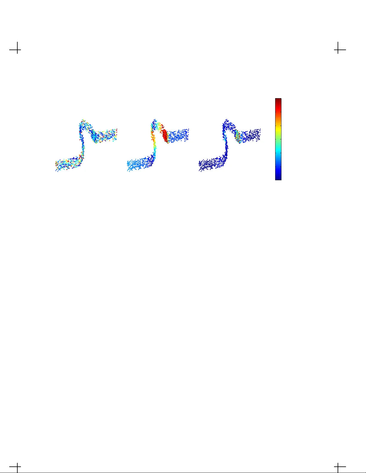
Information and Infer ence: A Journal of the IMA (2018) Page 1 of 53 doi:10.1093/imaiai/drn000 Non-Asymptotic Analysis of T angent Space Perturbation D A N I E L N . K A S L OV S K Y ∗ A N D F R A N C ¸ O I S G . M E Y E R Department of Applied Mathematics, University of Colorado, Boulder , Boulder , CO, USA ∗ kaslovsk y@colorado.edu fmeyer@colorado.edu [Receiv ed on 28 June 2018] Constructing an efﬁcient parameterization of a large, noisy data set of points lying close to a smooth manifold in high dimension remains a fundamental problem. One approach consists in recovering a local parameterization using the local tangent plane. Principal component analysis (PCA) is often the tool of choice, as it returns an optimal basis in the case of noise-free samples from a linear subspace. T o process noisy data samples from a nonlinear manifold, PCA must be applied locally , at a scale small enough such that the manifold is approximately linear , but at a scale large enough such that structure may be discerned from noise. Using eigenspace perturbation theory and non-asymptotic random matrix theory , we study the stability of the subspace estimated by PCA as a function of scale, and bound (with high probability) the angle it forms with the true tangent space. By adaptiv ely selecting the scale that minimizes this bound, our analysis rev eals an appropriate scale for local tangent plane recovery . W e also introduce a geometric uncertainty principle quantifying the limits of noise-curvature perturbation for stable recovery . With the purpose of providing perturbation bounds that can be used in practice, we propose plug-in estimates that make it possible to directly apply the theoretical results to real data sets. K eywor ds : manifold-valued data, tangent space, principal component analysis, subspace perturbation, local linear models, curvature, noise. 2000 Math Subject Classiﬁcation: 62H25, 15A42, 60B20 1. Introduction and Overview of the Main Results 1.1 Local T angent Space Recovery: Motivation and Goals Large data sets of points in high-dimension often lie close to a smooth low-dimensional manifold. A fundamental problem in processing such data sets is the construction of an ef ﬁcient parameterization that allows for the data to be well represented in fe wer dimensions. Such a parameterization may be realized by exploiting the inherent manifold structure of the data. Howe ver , discov ering the geometry of an underlying manifold from only noisy samples remains an open topic of research. The case of data sampled from a linear subspace is well studied (see [16, 18, 31], for e xample). The optimal parameterization is gi ven by principal component analysis (PCA), as the singular v alue decom- position (SVD) produces the best lo w-rank approximation for such data. Howe ver , most interesting manifold-valued data organize on or near a nonlinear manifold. PCA, by projecting data points onto the linear subspace of best ﬁt, is not optimal in this case as curvature may only be accommodated by choos- ing a subspace of dimension higher than that of the manifold. Algorithms designed to process nonlinear data sets typically proceed in one of two directions. One approach is to consider the data globally and produce a nonlinear embedding. Alternativ ely , the data may be considered in a piece wise-linear f ashion and linear methods such as PCA may be applied locally . The latter is the subject of this work. Local linear parameterization of manifold-valued data requires the estimation of the local tangent c  The author 2018. Published by Oxford University Press on behalf of the Institute of Mathematics and its Applications. All rights reserved. 2 of 53 D. N. KASLO VSKY AND F . G. MEYER 0 10 20 30 40 50 60 70 80 90 (a) small neighborhoods 0 10 20 30 40 50 60 70 80 90 (b) large neighborhoods Angle (degrees) 0 15 30 45 60 75 90 (c) adaptive neighborhoods F I G . 1. Angle between estimated and true tangent planes at each point of a noisy 2-dimensional data set embedded in R 3 . The estimated tangent planes are (a) randomly oriented when computed from small neighborhoods within the noise; (b) misaligned when computed from large neighborhoods e xhibiting curvature; and (c) properly oriented when computed from adaptively deﬁned neighborhoods giv en by the analysis in this work. space (“tangent plane”) from a neighborhood of points. Ho wev er , sample points are often corrupted by high-dimensional noise and any local neighborhood deviates from the linear assumptions of PCA due to the curv ature of the manifold. Therefore, the subspace reco vered by local PCA is a perturbed v ersion of the true tangent space. The goal of the present work is to characterize the stability and accuracy of local tangent space estimation using eigenspace perturbation theory . The proper neighborhood for local tangent space reco very must be a function of intrinsic (manifold) dimension, curvature, and noise lev el; these properties often v ary as different regions of the manifold are explored. Howe ver , local PCA approaches proposed in the data analysis and manifold learning literature often deﬁne locality via an a priori ﬁxed number of neighbors or as the output of clustering and partitioning algorithms (e.g., [19, 34, 48, 50]). Other methods [1, 25, 33] adaptively estimate local neighborhood size but are not tuned to the perturbation of the recov ered subspace. Our approach studies this perturbation as the size of the neighborhood varies to guide the deﬁnition of locality . On the one hand, a neighborhood must be small enough so that it is approximately linear and avoids curv ature. On the other hand, a neighborhood must be be large enough to overcome the ef fects of noise. A simple yet instructiv e example of these competing criteria is shown in Figure 1. The tangent plane at every point of a noisy 2-dimensional data set embedded in R 3 is computed via local PCA. Each point is color coded according to the angle formed with the true tangent plane. Three dif ferent neighborhood deﬁnitions are used: a small, ﬁxed radius (Figure 1a); a large, ﬁxed radius (Figure 1b); and radii deﬁned adaptiv ely according to the analysis presented in this w ork (Figure 1c). As small neighborhoods may be within the noise level and large neighborhoods exhibit curvature, the ﬁgure shows that neither allows for accurate tangent plane reco very . In fact, because the curv ature v aries across the data, only the adapti vely deﬁned neighborhoods av oid random orientation due to noise (as seen in Figure 1a) and misalignment due to curvature (as seen in Figure 1b). Figure 1c shows accurate and stable recov ery at almost ev ery data point, with misalignment only in the small region of very high curvature that will be troublesome for any method. The present work quantiﬁes this observed beha vior in the high-dimensional setting. W e present a non-asymptotic, eigenspace perturbation analysis to bound, with high probability , the T ANGENT SP A CE PER TURB A TION 3 of 53 angle between the recov ered linear subspace and the true tangent space as the size of the local neighbor - hood varies. The analysis accurately tracks the subspace recov ery error as a function of neighborhood size, noise, and curvature. Thus, we are able to adaptiv ely select the neighborhood that minimizes this bound, yielding the best estimate to the local tangent space from a large but ﬁnite number of noisy manifold samples. Further , the behavior of this bound demonstrates the non-trivial existence of such an optimal scale. W e also introduce a geometric uncertainty principle quantifying the limits of noise- curvature perturbation for tangent space reco very . An important technical matter that one needs to address when analyzing points that are sampled from a manifold blurred with Gaussian noise concerns the probability distrib ution of the noisy samples. Indeed, after perturbation with Gaussian noise, the probability density function of the noisy points can be expressed as the conv olution of the probability density function of the clean points on the manifold with a Gaussian kernel. Geometrically , the points are diffused into a tube around the manifold, and the corresponding density of the points is thinned. This concept has been studied in great detail in [26, 27] as well as in [12, 32]. The practical implication of these studies is that concentration of measure helps us to guarantee that the v olume of noisy points in a ball centered on the clean manifold can be estimated from the volume of the corresponding ball of clean points, provided one applies a correction of the radius. W e take advantage of these ideas in our analysis by replacing the ball of noisy points in the tube with a ball of similar volume extracted from the clean manifold, perturbed by Gaussian noise. W e introduce the resulting, necessary modiﬁcation to the radii in Section 5. A related issue concerns the determination of the point x 0 about which we estimate the tangent plane. From a practical perspectiv e, one can only observe noisy samples, and it is therefore reasonable that the perturbation bound should account for the fact that the analysis cannot be centered around the clean manifold. The expected ef fect of this additional source of uncertainty has been e xplored in detail in [26, 27]. In this paper , we propose a dif ferent approach. W e de vise a plug-in method to estimate a clean point x 0 on the manifold using the observed noisy data. As a result, the theoretical analysis can proceed assuming that x 0 is gi ven by an oracle. Our e xperiments conﬁrm that the local origin x 0 on the manifold can be estimated from the noisy neighborhood of observed points and that the perturbation error can be accurately tracked in practice. In addition, we expect this novel denoising algorithm to provide a universal tool for the analysis of noisy point cloud data. Our analysis is related to the very recent work of T yagi, et al. [43], in which neighborhood size and sampling density conditions are given to ensure a small angle between the PCA subspace and the true tangent space of a noise-free manifold. Results are e xtended to arbitrary smooth embeddings of the manifold model, which we do not consider . In contrast, we en vision the scenario in which no control is giv en o ver the sampling and explore the case of data sampled according to a ﬁxed density and corrupted by high-dimensional noise. Crucial to our results is a careful analysis of the interplay between the perturbation due to noise and the perturbation due to curvature. Nonetheless, our results can be shown to recover those of [43] in the noise-free setting. Our approach is also similar to the analysis presented by Nadler in [31], who studies the ﬁnite-sample properties of the PCA spectrum. Through matrix perturbation theory , [31] examines the angle between the leading ﬁnite-sample-PCA eigen vector and that of the leading population-PCA eigen vector . As a linear model is assumed, perturbation results from noise only . Despite this difference, the two analyses utilize similar techniques to bound the effects of perturbation on the PCA subspace and our results recov er those of [31] in the curvature-free setting. Application of multiscale PCA for geometric analysis of data sets has also been studied in [2, 9, 10, 46]. In parallel to our work [20–22, 28], Maggioni and coauthors have dev eloped results [3, 26, 27] addressing similar questions as those examined in this paper . These results are discussed above as well as in more detail in Section 5 and Section 6. Other recent related works include that of Singer and 4 of 53 D. N. KASLO VSKY AND F . G. MEYER W u [40], who use local PCA to build a tangent plane basis and gi ve an analysis for the neighborhood size to be used in the absence of noise. Using the hybrid linear model, Zhang, et al. [49] assume data are samples from a collection of “ﬂats” (afﬁne subspaces) and choose an optimal neighborhood size from which to recov er each ﬂat by studying the least squares approximation error in the form of Jones’ β -number (see [17] and also [7] in which this idea is used for curve denoising). Finally , an analysis of noise and curvature for normal estimation of smooth curves and surfaces in R 2 and R 3 is presented by Mitra, et al. [29] with application to computer graphics. 1.2 Overview of the Results W e consider the problem of recov ering the best approximation to a local tangent space of a nonlinear d -dimensional Riemannian manifold M from noisy samples presented in dimension D > d . W orking about a reference point x 0 , an approximation to the tangent space of M at x 0 is giv en by the span of the top d eigen vectors of the centered data cov ariance matrix (where “top” refers to the d eigen vectors or singular v ectors associated with the d largest eigen v alues or singular v alues). The question becomes: how many neighbors of x 0 should be used (or in how large of a radius about x 0 should we work) to recov er the best approximation? W e will often use the term “scale” to refer to this neighborhood size or radius. T o answer this question, we consider the perturbation of the eigen vectors spanning the estimated tangent space in the context of the “noise-curvature trade-off. ” T o balance the ef fects of noise and curvature (as observed in the example of the previous subsection, Figure 1), we seek a scale large enough to be above the noise lev el but still small enough to avoid curv ature. This scale reveals a linear structure that is suf ﬁciently decoupled from both the noise and the curv ature to be well approximated by a tangent plane. At this scale, the reco vered eigen vectors span a subspace corresponding very closely to the true tangent space of the manifold at x 0 . W e note that the concept of noise-curvature trade-of f has been a subject of interest for decades in dynamical systems theory [9]. The main result of this work is a bound on the angle between the computed and true tangent spaces. Deﬁne P to be the orthogonal projector onto the true tangent space and let b P be the orthogonal projector constructed from the d -dimensional eigenspace of the neighborhood cov ariance matrix. Then the dis- tance k P − b P k 2 F corresponds to the sum of the squared sines of the principal angles between the computed and true tangent spaces and we use eigenspace perturbation theory to bound this norm. Momentarily neglecting probability-dependent constants to ease the presentation, the ﬁrst-order approximation of this bound has the following form: Informal Main Result. k P − b P k F 6 2 √ 2 √ N  K (+) r 3 + σ p d ( D − d )  σ + r √ d + 2 + K 1 / 2 r 2 ( d + 2 ) √ 2 ( d + 4 )  r 2 d + 2 − K r 4 2 ( d + 2 ) 2 ( d + 4 ) − σ 2  √ d + √ D − d  , (1.1) where r is the radius (measured in the tangent plane) of the neighborhood containing N points, σ is the noise lev el, and K (+) and K are functions of curvature. T o aid the interpretation, we note that K (+) corresponds to the Frobenius norm of the matrix of principal curvatures and K has size 2 d ( D − d ) κ 2 in the case where all principal curv atures are equal to κ . The quantities N , r , σ , K (+) , and K , as well as the sampling assumptions are more formally deﬁned in Sections 2 and 3, and the formal result is presented in Section 3. T ANGENT SP A CE PER TURB A TION 5 of 53 The denominator of this bound, denoted here by δ informal , δ informal = r 2 d + 2 − K r 4 2 ( d + 2 ) 2 ( d + 4 ) − σ 2  √ d + √ D − d  (1.2) quantiﬁes the separation between the spectrum of the linear subspace ( ≈ r 2 ) and the perturbation due to curvature ( ≈ K r 4 ) and noise ( ≈ σ 2 ( √ d + √ D − d ) ). Clearly , we must have δ informal > 0 to approximate the appropriate linear subspace, a requirement made formal by Theorem 3.1 in Section 3. In general, when δ informal is zero (or negati ve), the bound becomes inﬁnite (or negati ve) and is not useful for sub- space recov ery . Howe ver , the geometric information encoded by (1.1) of fers more insight. For example, we observe that a small δ informal indicates that the estimated subspace contains a direction orthogonal to the true tangent space (due to the curv ature or noise). W e therefore consider δ informal to be the condition number for subspace recov ery and use it to dev elop our geometric interpretation for the bound. The noise-curvature trade-off is readily apparent from (1.1). The linear and curvature contrib utions are small for small v alues of r . Thus for a small neighborhood ( r small), the denominator (1.2) is either negati ve or ill conditioned for most values of σ and the bound becomes large. This matches our intuition as we hav e not yet encountered much curv ature but the linear structure has also not been explored. Therefore, the noise dominates the early behavior of this bound and an approximating subspace may not be recov ered from noise. As the neighborhood radius r increases, the conditioning of the denominator improv es, and the bound is controlled by the 1 / √ N behavior of the numerator . This again corresponds with our intuition: the addition of more points serves to ov ercome the effects of noise as the linear structure is explored. Thus, when δ − 1 informal is well conditioned, the bound on the angle may become smaller with the inclusion of more points. Eventually r becomes large enough such that the curv ature contribution approaches the size of the linear contribution and δ − 1 informal becomes large. The 1 / √ N term is ov ertaken by the ill conditioning of the denominator and the bound is again forced to become large. The noise-curvature trade-off, seen analytically here in (1.1) and (1.2), will be demonstrated numerically in Section 4. Enforcing a well conditioned recov ery bound (1.1) yields a geometric uncertainty principle quanti- fying the amount of curvature and noise we may tolerate. T o recover an approximating subspace, we must hav e: Geometric Uncertainty Principle. K σ 2 < d + 4 2 ( √ d + √ D − d ) (1.3) By prev enting the curvature and noise level from simultaneously becoming large, this requirement ensures that the linear structure of the data is recoverable. With high probability , the noise component normal to the tangent plane concentrates on a sphere with mean curv ature 1 / ( σ √ D − d ) . As will be shown, this uncertainty principle expresses the intuitiv e notion that the curvature of the manifold must be less than the curvature of this noise-ball. Otherwise, the combined effects of noise and curv ature perturbation prev ent an accurate estimate of the local tangent space. W e note that the concept of a geometric uncertainty principle also appears in the context of the computation of the homology of the manifold M in [32]. As explained in detail in Section 3.2, the two principles are strikingly similar . The remainder of the paper is organized as follows. Section 2 provides the notation, geometric model, and necessary mathematical formulations used throughout this work. Eigenspace perturbation 6 of 53 D. N. KASLO VSKY AND F . G. MEYER theory is revie wed in this section. The main results are stated formally in Section 3. W e demonstrate the accurac y of our results and test the sensiti vity to errors in parameter estimation in Section 4. Section 5 presents the modiﬁcations that are needed to account for the sampling density of the noisy points, and introduces two plug-in estimates that can be used in practice to apply the theoretical results of Section 3 to a real data set. W e conclude in Section 6 with a discussion of the relationship to pre viously established results and further algorithmic considerations. T echnical results and proofs are presented in the appendices. 2. Mathematical Preliminaries 2.1 Geometric Data Model A d -dimensional Riemannian manifold of codimension 1 may be described locally about a reference point x 0 by the surface y = f ( ` 1 , . . . , ` d ) , where ` i is a coordinate in the tangent plane, T x 0 M , to the manifold at x 0 . After translating x 0 to the origin, we hav e x 0 = [ 0 0 · · · 0 ] T , and a rotation of the coordinate system can align the coordinate axes with the principal directions asso- ciated with the principal curv atures at x 0 . Aligning the coordinate axes with the plane tangent to M at x 0 giv es a local quadratic approximation to the manifold. Using this choice of coordinates, the manifold may be described locally [13] by the T aylor series of f at x 0 : y = f ( ` 1 , . . . , ` d ) = 1 2 ( κ 1 ` 2 1 + · · · + κ d ` 2 d ) + o  ` 2 1 + · · · + ` 2 d  , (2.1) where κ 1 , . . . , κ d are the principal curvatures of M at x 0 . In this coordinate system, a point x in a neighborhood of x 0 has the form x = [ ` 1 ` 2 · · · ` d f ( ` 1 , . . . , ` d )] T . Generalizing to a d -dimensional manifold of arbitrary codimension in R D , there exist ( D − d ) functions f i ( ` ) = 1 2 ( κ ( i ) 1 ` 2 1 + · · · + κ ( i ) d ` 2 d ) + o  ` 2 1 + · · · + ` 2 d  , (2.2) for i = ( d + 1 ) , . . . , D , with κ ( i ) 1 , . . . , κ ( i ) d representing the principal curv atures in the i th normal direction at x 0 . Then, giv en the coordinate system aligned with the principal directions, a point in a neighbor- hood of x 0 has coordinates [ ` 1 , . . . , ` d , f d + 1 , . . . , f D ] . W e truncate the T aylor expansion (2.2) and use the quadratic approximation f i ( ` ) = 1 2 ( κ ( i ) 1 ` 2 1 + · · · + κ ( i ) d ` 2 d ) , (2.3) i = ( d + 1 ) , . . . , D , to describe the manifold locally . Consider now discrete samples from M obtained by uniformly sampling the ﬁrst d coordinates ( ` 1 , . . . , ` d ) in the tangent space inside B d x 0 ( r ) , the d -dimensional ball of radius r centered at x 0 , with the remaining ( D − d ) coordinates given by (2.3). Because we are sampling from a noise-free linear subspace, the number of points N captured inside B d x 0 ( r ) is a function of the sampling density ρ : N = ρ v d r d , (2.4) T ANGENT SP A CE PER TURB A TION 7 of 53 where v d is the v olume of the d -dimensional unit ball. The sampled points are assumed to be in general linear position, a standard assumption when sampling from a linear subspace (see Remark 2.3). Finally , we assume the sample points of M are contaminated with an additiv e Gaussian noise vector e drawn from the N  0 , σ 2 I D  distribution. Each sample x is a D -dimensional vector , and N such samples may be stored as columns of a matrix X ∈ R D × N . The coordinate system above allo ws the decomposition of x into its linear (tangent plane) component ` , its quadratic (curvature) component c , and noise e , three D -dimensional vectors ` = [ ` 1 ` 2 · · · ` d 0 · · · 0 ] T (2.5) c = [ 0 · · · 0 c d + 1 · · · c D ] T (2.6) e = [ e 1 e 2 · · · e D ] T (2.7) such that the last ( D − d ) entries of c are of the form c i = f i ( ` ) , i = ( d + 1 ) , . . . , D . W e may store the N samples of ` , c , and e as columns of matrices L , C , E , respecti vely , such that our data matrix is decomposed as X = L + C + E . (2.8) The true tangent space we wish to recover is gi ven by the PCA of L . Because we do not have direct access to L , we work with X as a proxy , and instead recover a subspace spanned by the corresponding eigen vectors of X X T . W e will study how close this recov ered inv ariant subspace of X X T is to the corresponding inv ariant subspace of LL T as a function of scale. Throughout this work, scale refers to the number of points N in the local neighborhood within which we perform PCA. Gi ven a ﬁx ed density of points, scale may be equiv alently quantiﬁed as the radius r about the reference point x 0 deﬁning the local neighborhood. R E M A R K 2.1 Of course it is unrealistic for the data to be observed in the described coordinate system. As noted, we may use a rotation to align the coordinate axes with the principal directions associated with the principal curvatures. Doing so allows us to write (2.3) as well as (2.8). Because we will ultimately quantify the norm of each matrix using the unitarily-in variant Frobenius norm, this rotation will not affect our analysis. W e therefore proceed by assuming that the coordinate axes align with the principal directions. R E M A R K 2.2 Equation (2.3) represents an exact quadratic embedding of M . While it may be interest- ing to consider more general embeddings, as is done for the noise-free case in [43], a T aylor expansion followed by rotation and translation will result in an embedding of the form (2.2). Noting that the numerical results of [43] indicate no loss in accuracy when truncating higher-order terms, proceeding with an analysis of (2.3) remains sufﬁciently general. R E M A R K 2.3 In a non-pathological conﬁguration (e.g., points observed in general linear position), only d + 1 sample points are needed to ensure that the top d eigenv ectors of LL T span the true tangent space. It has been noted in the literature (e.g., [38, 44]) that O ( d log d ) points should be sampled for the empirical cov ariance matrix to be close in norm to the population cov ariance, with high probability . Strictly enforcing this sampling condition is a very mild requirement for our setting, in which the sampling density ρ (see equation (2.4)) is usually large and the extra logarithmic factor of d is easily achiev ed. Further , this logarithmic factor is implicitly present in our analysis as a consequence of the lo wer bound on the smallest eigenv alue of L L T (see Appendix A.1). W e also note that we do not intend to analyze the extremely small scales (very small N ) where ﬁnite sample ef fects create instability and prev ent a meaningful analysis. 8 of 53 D. N. KASLO VSKY AND F . G. MEYER 2.2 P erturbation of Invariant Subspaces Giv en the decomposition of the data (2.8), we hav e X X T = LL T + CC T + E E T + L C T + C L T + LE T + E L T + C E T + E C T . (2.9) W e introduce some notation to account for the centering required by PCA. Deﬁne the sample mean of N realizations of random vector m as m = 1 N N ∑ i = 1 m ( i ) , (2.10) where m ( i ) denotes the i th realization. Letting 1 N represent the column vector of N ones, deﬁne M = m 1 T N (2.11) to be the matrix with N copies of m as its columns. Finally , let e M denote the centered version of M : e M = M − M . (2.12) Then we hav e e X e X T = e L e L T + e C e C T + e E e E T + e L e C T + e C e L T + e L e E T + e E e L T + e C e E T + e E e C T . (2.13) The problem may be posed as a perturbation analysis of in v ariant subspaces. Rewrite (2.9) as 1 N e X e X T = 1 N e L e L T + ∆ , (2.14) where ∆ = 1 N ( e C e C T + e E e E T + e L e C T + e C e L T + e L e E T + e E e L T + e C e E T + e E e C T ) (2.15) is the perturbation that prev ents us from working directly with e L e L T . The dominant eigenspace of e X e X T is therefore a perturbed version of the dominant eigenspace of e L e L T . Seeking to minimize the effect of this perturbation, we look for the scale N ∗ (equiv alently r ∗ ) at which the dominant eigenspace of e X e X T is closest to that of e L e L T . Before proceeding, we revie w material on the perturbation of eigenspaces relev ant to our analysis. The reader familiar with this topic is in vited to skip directly to Theorem 2.1. The distance between two subspaces of R D can be deﬁned as the spectral norm of the dif ference between their respectiv e orthogonal projectors [15]. As we will always be considering two equidimen- sional subspaces, this distance is equal to the sine of the largest principal angle between the subspaces. T o control all such principal angles, we state our results using the Frobenius norm of this difference. Our goal is therefore to control the behavior of k P − b P k F , where P and b P are the orthogonal projectors onto the subspaces computed from L and X , respectiv ely . The norm k P − b P k F may be bounded by the classic sin Θ theorem of Davis and Kahan [4]. W e will use a version of this theorem presented by Stew art (Theorem V .2.7 of [41]), modiﬁed for our speciﬁc purpose. First, we establish some notation, following closely that found in [41]. Consider the eigendecompositions 1 N e L e L T = U Λ U T = [ U 1 U 2 ]  Λ 1 Λ 2  [ U 1 U 2 ] T , (2.16) 1 N e X e X T = b U b Λ b U T = [ b U 1 b U 2 ] " b Λ 1 b Λ 2 # [ b U 1 b U 2 ] T , (2.17) T ANGENT SP A CE PER TURB A TION 9 of 53 such that the columns of U are the eigenv ectors of 1 N e L e L T and the columns of b U are the eigenv ectors of 1 N e X e X T . The eigen v alues of 1 N e L e L T are arranged in descending order as the entries of diagonal matrix Λ . The eigen values are also partitioned such that diagonal matrices Λ 1 and Λ 2 contain the d largest entries of Λ and the ( D − d ) smallest entries of Λ , respectiv ely . The columns of U 1 are those eigenv ectors associated with the d eigen v alues in Λ 1 , the columns of U 2 are those eigenv ectors associated with the ( D − d ) eigen values in Λ 2 , and the eigendecomposition of 1 N e X e X T is similarly partitioned. The subspace we recover is spanned by the columns of b U 1 and we wish to ha ve this subspace as close as possible to the tangent space spanned by the columns of U 1 . The orthogonal projectors onto the tangent and computed subspaces, P and b P respectiv ely , are giv en by P = U 1 U T 1 and b P = b U 1 b U T 1 . Deﬁne λ d to be the d th largest eigen value of 1 N e L e L T , or the last entry on the diagonal of Λ 1 . This eigen v alue corresponds to variance in a tangent space direction. W e are no w in position to state the theorem. Note that we hav e made use of the fact that the columns of U are the eigen vectors of e L e L T , that Λ 1 , Λ 2 are Hermitian (diagonal) matrices, and that the Frobenius norm is used to measure distances. The reader is referred to [41] for the theorem in its original form. T H E O R E M 2.1 (Davis & Kahan [4], Ste wart [41]) Let δ = λ d −   U T 1 ∆ U 1   F −   U T 2 ∆ U 2   F and consider • (Condition 1) δ > 0 • (Condition 2)   U T 1 ∆ U 2   F   U T 2 ∆ U 1   F < 1 4 δ 2 . Then, provided that conditions 1 and 2 hold,    P − b P    F 6 2 √ 2   U T 2 ∆ U 1   F δ . (2.18) It is instructive to consider the perturbation ∆ as an operator with range in R D and quantify its ef fect on the existing inv ariant subspaces. Consider ﬁrst the idealized case where U 1 is an inv ariant subspace of ∆ , i.e., ∆ maps points from the column space of U 1 to the column space of U 1 . Clearly , U T 2 ∆ U 1 = 0 in this case as the subspace spanned by U 1 remains in variant under the action of ∆ , and the perturbation angle is zero. In general, howe ver , we cannot expect such an idealized restriction for the range of ∆ and we therefore expect that ∆ U 1 will have a component that is normal to the tangent space. The numerator k U T 2 ∆ U 1 k F of (2.18) measures this normal component, thereby quantifying the effect of the perturbation on the tangent space. Then k U T 1 ∆ U 1 k F measures the component that remains in the tangent space after the action of ∆ . As this component does not contain curv ature, k U T 1 ∆ U 1 k F corresponds to the spectrum of the noise projected in the tangent space. Similarly , k U T 2 ∆ U 2 k F measures the spectrum of the curvature and noise perturbation normal to the tangent space. Thus, when ∆ leaves the column space of U 1 mostly unperturbed (i.e., k U T 2 ∆ U 1 k F is small) and the spectrum of the tangent space is well separated from that of the noise and curv ature, the estimated subspace will form only a small angle with the true tangent space. In the ne xt section, we use the machinery of this classic result to bound the angle caused by the perturbation ∆ and dev elop an interpretation of the conditions of Theorem 2.1 suited to the noise-curvature trade-of f. 10 of 53 D. N. KASLO VSKY AND F . G. MEYER 3. Main Results Giv en the framework for analysis developed above, the terms appearing in the statement of Theorem 2.1 (   U T 1 ∆ U 1   F ,   U T 2 ∆ U 2   F ,   U T 2 ∆ U 1   F ,   U T 1 ∆ U 2   F , and λ d ) must be controlled. W e notice that ∆ is a symmetric matrix, so that   U T 1 ∆ U 2   F =   U T 2 ∆ U 1   F . Using the triangle inequality and the geometric constraints U T 1 C = 0 and U T 2 L = 0 , (3.1) the norms may be controlled by bounding the contribution of each term in the perturbation ∆ :   U T 1 ∆ U 1   F 6 2     U T 1 1 N e L e E T U 1     F +     U T 1 1 N e E e E T U 1     F ,   U T 2 ∆ U 2   F 6     U T 2 1 N e C e C T U 2     F + 2     U T 2 1 N e C e E T U 2     F +     U T 2 1 N e E e E T U 2     F ,   U T 2 ∆ U 1   F 6     U T 2 1 N e C e L T U 1     F +     U T 2 1 N e E e L T U 1     F +     U T 2 1 N e C e E T U 1     F +     U T 2 1 N e E e E T U 1     F . Importantly , we seek control o ver each (right-hand side) term in the ﬁnite-sample regime, as we assume a possibly large but ﬁnite number of sample points N . Therefore, bounds are deriv ed through a careful analysis employing concentration results and techniques from non-asymptotic random matrix theory . The technical analysis is presented in the appendix and proceeds by analyzing three distinct cases: the cov ariance of bounded random matrices, unbounded random matrices, and the interaction of bounded and unbounded random matrices. The eigenv alue λ d is bounded again using random matrix theory . In all cases, care is taken to ensure that bounds hold with high probability that is independent of the ambient dimension D . R E M A R K 3.1 Other , possibly tighter , av enues of analysis may be possible for some of the bounds pre- sented in the appendix. Howe v er , the presented analysis avoids lar ge union bounds and dependence on the ambient dimension to state results holding with high probability . Alternati ve analyses are possible, often sacriﬁcing probability to exhibit sharper concentration. W e proceed with a theoretical analysis holding with the highest probability while maintaining accurate results. 3.1 Bounding the Angle Between Subspaces W e are now in position to apply Theorem 2.1 and state our main result. First, we make the follo wing deﬁnitions in volving the principal curv atures: K i = d ∑ n = 1 κ ( i ) n , K = D ∑ i = d + 1 K 2 i ! 1 2 , (3.2) K i j nn = d ∑ n = 1 κ ( i ) n κ ( j ) n , K i j mn = d ∑ m , n = 1 m 6 = n κ ( i ) m κ ( j ) n , (3.3) and K = " D ∑ i = d + 1 D ∑ j = d + 1  ( d + 1 ) K i j nn − K i j mn  2 # 1 2 . (3.4) T ANGENT SP A CE PER TURB A TION 11 of 53 The constant K i is the mean curvature (rescaled by a factor of d ) in normal direction i , for ( d + 1 ) 6 i 6 D . The curv ature of the local model is quantiﬁed by K , which is a natural result of our use of the Frobenius norm, and K , which results from the expectation of the norm of the curvature covariance. Note that K i K j = K i j nn + K i j mn . W e also deﬁne the constants K (+) i = d ∑ n = 1 | κ ( i ) n | 2 ! 1 2 , and K (+) = D ∑ i = d + 1 ( K (+) i ) 2 ! 1 2 (3.5) to be used when strictly positiv e curv ature terms are required. The main result is formulated in the appendix and makes the follo wing benign assumptions on the number of sample points N and the probability constants ξ and ξ λ : N > 4 ( max ( √ d , √ D − d ) + ξ ) , ξ < 0 . 7 p d ( D − d ) , and ξ λ < 3 √ d + 2 √ N , in addition to the requirement that N > O ( d log d ) for the points observ ed in general linear position (see Remark 2.3). W e note that the assumptions are easily satisﬁed as we en vision a sampling density such that N is large (but ﬁnite). Further, the assumptions listed above are not crucial to the result but allo w for a more compact presentation. T H E O R E M 3.1 (Main Result) Let δ = r 2 d + 2 − K r 4 2 ( d + 2 ) 2 ( d + 4 ) − σ 2  √ d + √ D − d  − 1 √ N ζ denom ( ξ , ξ λ ) (3.6) and β = 1 √ N  K (+) r 3 ν ( ξ ) + σ p d ( D − d ) η ( ξ , ξ λ ) + 1 √ N ζ numer ( ξ )  . (3.7) If the following conditions hold (in addition to the benign assumptions stated abo ve): • (Condition 1) δ > 0, • (Condition 2) β < 1 2 δ , then    P − b P    F 6 2 √ 2 β δ = 2 √ 2 1 √ N h K (+) r 3 ν ( ξ ) + σ p d ( D − d ) η ( ξ , ξ λ ) + 1 √ N ζ numer ( ξ ) i r 2 d + 2 − K r 4 2 ( d + 2 ) 2 ( d + 4 ) − σ 2  √ d + √ D − d  − 1 √ N ζ denom ( ξ , ξ λ ) (3.8) with probability greater than 1 − 2 d e − ξ 2 λ − 9 e − ξ 2 (3.9) ov er the joint random selection of the sample points and random realization of the noise, where the following deﬁnitions ha ve been made to ease the presentation: • geometric and noise terms ν ( ξ ) = 1 2 ( d + 3 ) ( d + 2 ) p 1 ( ξ ) , (linear–curv ature) 12 of 53 D. N. KASLO VSKY AND F . G. MEYER η 1 = σ , (noise) η 2 ( ξ λ ) = r √ d + 2 p 2 ( ξ λ ) , (linear–noise) η 3 ( ξ ) = K 1 / 2 r 2 ( d + 2 ) p 2 ( d + 4 ) p 5 ( ξ ) , (curvature–noise) η ( ξ , ξ λ ) = p 3 ( ξ , p d ( D − d ))  η 1 + η 2 ( ξ λ ) + η 3 ( ξ )  , • ﬁnite sample correction terms (numerator) ζ 1 ( ξ ) = 1 2 K (+) r 3 p 2 1 ( ξ ) , (linear–curv ature) ζ 2 ( ξ ) = σ 2 p d ( D − d ) p 3 ( ξ , p d ( D − d )) p 4 ( ξ , √ D − d ) , (noise) ζ numer ( ξ ) = ζ 1 ( ξ ) + ζ 2 ( ξ ) , • ﬁnite sample correction terms (denominator) ζ 3 ( ξ λ ) = r 2 d + 2  p 0 ( ξ λ ) +  2 √ N − 1 N 3 / 2   1 − p 0 ( ξ λ ) √ N  , (linear) ζ 4 ( ξ ) = ( K (+) ) 2 r 4 4  p 1 ( ξ ) + 1 √ N p 2 1 ( ξ )  , (curvature) ζ 5 ( ξ , ξ λ ) = 2 r σ d √ d + 2 p 2 ( ξ λ ) p 3 ( ξ , d ) , (linear–noise) ζ 6 ( ξ ) = 2 K 1 2 r 2 σ ( D − d ) ( d + 2 ) p 2 ( d + 4 ) p 3 ( ξ , D − d ) p 5 ( ξ ) , (curvature–noise) ζ 7 ( ξ ) = 5 2 σ 2 h √ d p 4 ( ξ , √ d ) + √ D − d p 4 ( ξ , √ D − d ) i , (noise) ζ denom ( ξ , ξ λ ) = ζ 3 ( ξ ) + ζ 4 ( ξ ) + ζ 5 ( ξ , ξ λ ) + ζ 6 ( ξ ) + ζ 7 ( ξ ) , and • probability-dependent terms (i.e., terms depending on the probability constants) p 0 ( ξ ) = ξ p 8 ( d + 2 ) ( 1 − 1 N ) , p 1 ( ξ ) =  2 + ξ √ 2  , p 2 ( ξ ) =  1 + ξ 5 √ d + 2 √ N  , p 3 ( ξ , ω ) =  1 + 6 5 ξ ω  , p 4 ( ξ , ω ) =  ω + ξ √ 2  , p 5 ( ξ ) = 1 + 1 √ N ( K (+) ) 2 2 K ( d + 2 ) 2 ( d + 4 )( p 1 ( ξ ) + 1 √ N p 2 1 ( ξ )) ! 1 / 2 . T ANGENT SP A CE PER TURB A TION 13 of 53 Finally , we recall the relationship N = ρ v d r d giv en by (2.4). Pr oof. Condition 2 is simpliﬁed from its original statement in Theorem 2.1 by noticing that ∆ is a symmetric matrix so that   U T 1 ∆ U 2   F =   U T 2 ∆ U 1   F . Then, applying the norm bounds computed in the appendix to Theorem 2.1 and choosing the probability constants ξ λ d = ξ λ 1 = ξ λ and ξ cc = ξ c ` = ξ e ` = ξ ce = ξ e 1 = ξ e 2 = ξ e 3 = ξ c = ξ (3.10) yields the result.  The bound (3.8) will be demonstrated in Section 4 to accurately track the angle between the true and computed tangent spaces at all scales. W e experimentally observe that the bound is, in general, either decreasing (for the curv ature-free case), increasing (for the noise-free case), or decreasing at small scales and increasing at large scales (for the general case). W e therefore expect to be able to locate a scale at which the bound is minimized. Based on this observation, the optimal scale, N ∗ , for tangent space recov ery may be selected as the N for which (3.8) is minimized (an equiv alent notion of the optimal scale may be gi ven in terms of the neighborhood radius r ). Note that the constants ξ and ξ λ need to be selected to ensure that this bound holds with high probability . For e xample, setting ξ = 2 and ξ λ = 2 . 75 yields probabilities of 0.81, 0.80, and 0.76 when d = 3 , 10 , and 50, respectiv ely . W e also note that the probability giv en by (3.9) is more pessimistic than we expect in practice. As introduced in Section 1.2, we may interpret δ − 1 as the condition number for tangent space recov ery . Noting that the denominator in (3.8) is a lower bound on δ , we analyze the condition number via the bounds for λ d , k U T 1 ∆ U 1 k F , and k U T 2 ∆ U 2 k F . Using these bounds in the Main Result (3.8), we see that when δ − 1 is small, we recover a tight approximation to the true tangent space. Like wise, when δ − 1 becomes large, the angle between the computed and true subspaces becomes large. The notion of an angle loses meaning as δ − 1 tends to inﬁnity , and we are unable to recover an approximating subspace. Condition 1, requiring that the denominator be bounded away from zero, has an important geo- metric interpretation. As noted abov e, the conditioning of the subspace recovery problem improv es as δ becomes large. Condition 1 imposes that the spectrum corresponding to the linear subspace ( λ d ) be well separated from the spectra of the noise and curvature perturbations encoded by k U T 1 ∆ U 1 k F + k U T 2 ∆ U 2 k F . In this way , condition 1 quantiﬁes our requirement that there exists a scale such that the linear subspace is sufﬁciently decoupled from the effects of curvature and noise. When the spectra are not well separated, the angle between the subspaces becomes ill deﬁned. In this case, the approximat- ing subspace contains an eigenv ector corresponding to a direction orthogonal to the true tangent space. Condition 2 is a technical requirement of Theorem 2.1. Provided that condition 1 is satisﬁed, we observe that a sufﬁcient sampling density will ensure that Condition 2 is met. Further , we numerically observe that the Main Result (3.8) accurately tracks the subspace recov ery error e ven in the case when condition 2 is violated. In such a case, the bound may not remain as tight as desired but its behavior at all scales remains consistent with the subspace recov ery error tracked in our experiments. Before numerically demonstrating our main result, we quantify the separation needed between the linear structure and the noise and curvature with a geometric uncertainty principle. 3.2 Geometric Uncertainty Principle for Subspace Recovery Condition 1 indeed imposes a geometric requirement for tangent space recovery . Solving for the range of scales for which condition 1 is satisﬁed and requiring the solution to be real yields the geometric uncertainty principle (1.3) stated in Section 1.2. W e note that this result is deriv ed using δ informal , deﬁned in equation (1.2), as the full expression for δ does not allow for an algebraic solution. 14 of 53 D. N. KASLO VSKY AND F . G. MEYER The geometric uncertainty principle (1.3) e xpresses a natural requirement for the subspace recov ery problem, ensuring that the perturbation to the tangent space is not too large. Recall that, with high probability , the noise orthogonal to the tangent space concentrates on a sphere with mean curv ature 1 / ( σ √ D − d ) . W e therefore expect to require that the curvature of the manifold be less than the curva- ture of this noise-ball. T o compare the curv ature of the manifold to that of the noise-ball, consider the case where all principal curvatures of the manifold are equal, and denote them by κ . Then (1.3) requires that κ < 1 σ √ D − d v u u t d + 4 4 d  √ d + √ D − d  . (3.11) Noting that, for d > 1, we have d + 4 4 d  √ d + √ D − d  < 1 , we see that the uncertainty principle (1.3) indeed requires that the mean curvature of the manifold be less than that of the perturbing noise-ball. Intuitiv ely , we might expect that the uncertainty principle would be of the form (curvature) × ( noise-ball radius ) < 1 . Howe ver , (1.3) is, in fact, more restrictiv e than our intuition, as illustrated by (3.11). As only ﬁnite- sample corrections hav e been neglected in δ informal , (1.3) is of the correct order . Interestingly , this more restrictiv e requirement for tangent space recov ery is only accessible through the careful perturbation analysis presented above and an estimate obtained by a more naiv e analysis would be too lax. The authors in [32] present an algorithm to compute the homology of a manifold from a data set of noisy points. The authors assume that the data are clean samples from a manifold perturbed with ( D − d ) - dimensional Gaussian noise along the normal ﬁbers. In the context of our model, this is equivalent to removing the ﬁrst d components of the noise vector . The authors prov e that the algorithm computes, with high probability , the correct homology of M , provided that the noise variance σ 2 satisﬁes 1 R < 1 σ √ D − d c √ 9 − √ 8 9 √ 8 with c < 1 . (3.12) The parameter 1 / R is an upper bound on all the principal curv atures ( R is also known as the r each [8]). This condition is almost identical to (3.11). The geometric uncertainty principle (1.3) is clearly not an artifact of our analysis, but is deeply rooted in the geometric and topological understanding of noisy manifolds. 4. Experimental Results I: V alidating the Theory In this section we present an experimental study of the tangent space perturbation results given above. In particular , we demonstrate that the bound presented in the Main Result (Theorem 3.1) accurately tracks the subspace recov ery error at all scales. As this analytic result requires no decompositions of the data matrix, our analysis provides an efﬁcient means for obtaining the optimal scale for tangent space reco very . W e ﬁrst present a practical use of the Main Result, demonstrating its accuracy when the intrinsic dimensionality , curvature, and noise lev el are known. W e then experimentally test the stability of the bound when these parameters are only imprecisely av ailable, as is the case when they must be T ANGENT SP A CE PER TURB A TION 15 of 53 estimated from the data. Finally , we demonstrate the accurate estimation of the noise level and local curvature. 4.1 Subspace T racking and Recovery W e generate a data set sampled from a 3-dimensional manifold embedded in R 20 according to the local model (2.3) by uniformly sampling N = 1 . 25 × 10 6 points inside a ball of radius 1 in the tangent plane. Curvature and the standard de viation σ of the added Gaussian noise will be speciﬁed in each experiment. W e compare our bound with the true subspace recov ery error . The tangent plane at reference point x 0 is computed at each scale N via PCA of the N nearest neighbors of x 0 . The true subspace recovery error k P − b P k F is then computed at each scale. Note that computing the true error requires N SVDs. A “true bound” is computed by applying Theorem 2.1 after measuring each perturbation norm directly from the data. While no SVDs are required, this true bound utilizes information that is not practically av ailable and represents the best possible bound that we can hope to achieve. W e will compare the mean of the true error and mean of the true bound over 10 trials (with error bars indicating one standard deviation) to the bound giv en by our Main Result in Theorem 3.1, holding with probability greater than 0.8. For the experiments in this section, the bound (3.8) is computed with full knowledge of the necessary parameters. In our experience, we observe in practice (results not shown) that the deviation of the empirical eigen v alue λ d from its expectation is insigniﬁcant ov er the entire range of relev ant scales and therefore neglect its correction term (derived using a Chernoff bound in Appendix A.1) for the experiments. W e further note that kno wledge of d provides an exact expression for this expectation as no additional geometric information is encoded by λ d . As the principle curvatures are known, we compute a tighter bound for k U T 2 CL T U 1 k F using K in place of K (+) . Doing so only affects the height of the curve; its trend as a function of scale is unchanged. In practice, the important information is captured by tracking the trend of the true error regardless of whether it provides an upper bound to any random ﬂuctuation of the data. In fact, the numerical results indicate that an accurate tracking of error is possible ev en when condition 2 of Theorem 3.1 is violated. T able 1. Principal curvatures of the manifold for Figures 2b and 2c. κ ( j ) i i = 1 i = 2 i = 3 j = 4 , . . . , 6 3.0000 1.5000 1.5000 j = 7 , . . . , 20 1.6351 0.1351 0.1351 The results are displayed in Figure 2. Panel (a) sho ws the noisy ( σ = 0 . 01 ) curvature-free (linear subspace) result. As the only perturbation is due to noise, we expect the error to decay as 1 / √ N as the scale increases. The curves are shown on a logarithmic scale (for the Y -axis) and decrease monotoni- cally , indicating the expected decay . Our bound (green) accurately tracks the behavior of the true error (blue) and is nearly identical to the true bound (red). Panel (b) shows the results for a noise-free mani- fold with principal curvatures giv en in T able 1 such that K = 12 . 6025. Notice that three of the normal directions e xhibit high curv ature while the others are ﬂatter , gi ving a tube-like structure to the manifold. In this case, perturbation is due to curvature only and the error increases monotonically (ignoring the slight numerical instability at extremely small scales), as predicted in the discussion of Sections 1.2 and 3.1. Eventually , a scale is reached at which there is too much curvature and the bounds blo w up to inﬁnity . This corresponds exactly to where the true error plateaus at its maximum value, indicating that 16 of 53 D. N. KASLO VSKY AND F . G. MEYER −2 0 2 4 6 8 10 12 14 x 10 5 10 −4 10 −2 10 0 10 2 10 4 N k P − b P k F True bound True error Main Result (a) −2 0 2 4 6 8 10 12 14 x 10 5 10 −4 10 −2 10 0 10 2 10 4 10 6 10 8 N k P − b P k F True bound True error Main Result (b) −2 0 2 4 6 8 10 12 14 x 10 5 10 −4 10 −2 10 0 10 2 10 4 10 6 10 8 N k P − b P k F True bound True error Main Result (c) −2 0 2 4 6 8 10 12 14 x 10 5 10 −4 10 −2 10 0 10 2 10 4 10 6 10 8 N k P − b P k F True bound True error Main Result (d) F I G . 2. Norm of the perturbation using tangent plane radius r : (a) ﬂat manifold with noise, (b) curved (tube-like) manifold with no noise, (c) curv ed (tube-like) manifold with noise, (d) curved manifold with noise. Dashed vertical lines indicate minima of the curves. Note the logarithmic scale on the Y -axes. See text for discussion. the computed subspace is no w orthogonal to the true tangent space. In this case, condition 1 of Theorem 3.1 is violated as there is no longer separation between the linear and curvature spectra, δ − 1 becomes large, and our analysis predicts that the computed eigenspace contains a direction orthogonal to the true tangent space. Figure 2c shows the results for a noisy ( σ = 0 . 01) version of the manifold used in panel (b). Note that the error is large at small scales due to noise and large at large scales due to curv ature. At these scales the bounds are accordingly ill conditioned and track the behavior of the true error when well conditioned. Figure 2d shows the results for a manifold again with K = 12 . 6025, but with the principal curvatures equal in all normal directions ( κ ( j ) i = 1 . 0189 for i = 1 , . . . , 3 and j = 4 , . . . , 20), and noise ( σ = 0 . 01) is added. W e observe the same general behavior as seen in panel (c), but both the true error and the bounds remain well conditioned at larger scales. This is explained by the fact that higher curvature T ANGENT SP A CE PER TURB A TION 17 of 53 is encountered at smaller scales for the manifold corresponding to panel (c) but is not encountered until larger scales in panel (d). Similar results are shown in Figure 3 for a 2-dimensional, noise-free saddle ( κ ( 3 ) 1 = 3 , κ ( 3 ) 2 = − 3) embedded in R 3 , demonstrating an accurate bound for the case of principle curvatures of mix ed signs. The true bound (red) tightly tracks the true error (blue) and is tighter than our bound (green) in all cases except for the curvature-free setting, where a difference on the order of 10 − 3 is observed. This curvature-free bound may be understood by observing that the noise analysis is more precise than that for the curvature (see appendices) and that the height of the bound is controlled by the probability- dependent constants, which have been ﬁxed across all plots for consistency . In fact, it is possible to choose the probability-dependent constants much larger for the curvature-free setting without violating Condition 2. Doing so increases the height of the bound (green) to match the height of the “true bound” (red) curve (result not shown). Note that a similar increase for nonzero curvature results in a curve that violates Condition 2. In all of the presented experiments, the bound accurately tracks the behavior of the true error . In fact, the curves are shown to be parallel on a logarithmic scale, indicating that they differ only by mul- tiplicativ e constants. These observations further indicate that the triangle inequalities used in bounding the norms k U T m ∆ U n k F , m , n = { 1 , 2 } , are reasonably tight. As no matrix decompositions are needed to compute our bounds, we hav e efﬁciently tracked the tangent space recovery error . The dashed vertical lines in Figure 2 indicate the locations of the minima of the true error curv e (dashed blue) and the Main Result bound (dashed green). In general, we see agreement of the locations at which the minima occur, indicating the scale that will yield the optimal tangent space approximation. The minimum of the Main Result bound falls within a range of scales at which the true recovery error is stable. In particular, we note that when the location of the bound’ s minimum does not correspond with the minimum of the true error (such as in panel (d)), the discrepancy occurs at a range of scales for which the true error is quite ﬂat. In fact, in panel (d), the difference between the error at the computed optimal scale and the error at the true optimal scale is on the order of 10 − 2 . Thus the angle between the computed and true tangent spaces will be less than half of a degree and the computed tangent space is stable in this range of scales. For a large data set it is impractical to e xamine e very scale and one w ould instead most likely use a coarse sampling of scales. The true optimal scale w ould almost surely be missed by such a coarse sampling scheme. Our analysis indicates that despite missing the exact true optimum, we may recov er a scale that yields an approximation to within a fraction of a degree of the optimum. 4.2 Sensitivity to Err or in P arameters As is often the case in practice, parameters such as intrinsic dimension, curvature, and noise lev el are unknown and must be estimated from the data. It is therefore important to experimentally test the sensitivity of tangent space reco very to errors in parameter estimation. In the following experiments, we test the sensiti vity to each parameter by tracking the optimal scale as one parameter is v aried with the others held ﬁxed at their true values. For consistency across experiments, the optimal scale is reported in terms of neighborhood radius and denoted by r ∗ . The relationship between neighborhood radius r and number of sample points N is deﬁned by equation (2.4). In all experiments, we generate data sets sampled from a 4-dimensional manifold embedded in R 10 according to the local model (2.3). Figure 4 shows that the optimal scale r ∗ is sensiti ve to errors in the intrinsic dimension d . A data set is sampled from a noisy , bowl-shaped manifold with equal principal curv atures in all directions. W e set the noise level σ = 0 . 01 and the principal curvatures κ ( i ) j = 2 in panel (a) and κ ( i ) j = 3 in panel (b). 18 of 53 D. N. KASLO VSKY AND F . G. MEYER −1000 0 1000 2000 3000 4000 5000 6000 −1 −0.5 0 0.5 1 1.5 2 2.5 3 N k P − b P k F True bound True error Main Result F I G . 3. Bounds for a 2-dimensional saddle (noise free) with κ ( 3 ) 1 = 3 and κ ( 3 ) 2 = − 3. Noting that the true intrinsic dimension is d = 4, we test the sensitivity of r ∗ as d is varied. There are three axes in each panel of Figure 4: the neighborhood radius r on the abscissa; the angle k P − b P k F on the left ordinate; and the values used for the dimension d on the right ordinate. Our Main Result bound is sho wn in blue and tracks the subspace reco very error (angle, on the left ordinate) as a function of neighborhood radius r for the true values of d , σ and κ ( i ) j . Holding the noise and curvature ﬁxed, we then compute r ∗ using incorrect values for d ranging from d = 1 to d = 7. The green and red curves show the computed r ∗ for each value of d (on the right ordinate) according to the two ways to ﬁx curv ature while varying d : (1) hold the value of each κ ( i ) j ﬁxed, thereby allowing K to change with d (shown in green); or (2) hold K ﬁxed, necessitating that the κ ( i ) j change with d (shown in red). The Main Result bound (blue) indicates an optimal radius of r ∗ ≈ 0 . 45 in (a) and r ∗ ≈ 0 . 30 in (b). Ho wev er , the r ∗ computed using inaccurate estimates of d show great v ariation, ranging between a radius close to the optimum and a radius close to the size of the entire manifold. These experimental results indicate the importance of properly estimating the intrinsic dimension of the data. Next, the sensiti vity to error in the estimated noise lev el is shown to be mild in Figure 5. A data set is sampled from a noisy , bowl-shaped manifold with equal principal curvatures in all directions. The true values for the parameters are: d = 4, κ ( i ) j = 1 . 5, and σ = 0 . 025 in 5a; and d = 4, κ ( i ) j = 2, and σ = 0 . 05 in 5b . Our Main Result bound (blue) tracks the subspace recovery error (left ordinate) as a function of r (abscissa) using the true parameter values and indicates an optimal radius of r ∗ ≈ 0 . 55 and r ∗ ≈ 0 . 5 for (a) and (b), respectively . Holding the dimension and curv ature constant, we then compute r ∗ using incorrect values for σ ranging from σ = 0 to σ = 0 . 06. The green curve shows the computed r ∗ for each v alue of σ (on the right ordinate). In both 5a and 5b, the computed r ∗ remain close to the optimum as the noise lev el varies and are within the range of radii where the recovery is stable (as indicated by the Main Result bound in blue). This behavior is in agreement with our experimental observations (not shown) indicating that increasing the noise le vel reduces the range for stable recovery but leaves the minimum of the Main Result bound relatively unaltered. W e note that the range for stable recovery is smaller in (b) as is expected in the higher curv ature and noise setting. Finally , Figure 6 shows mild sensiti vity to error in estimated curv ature. A data set is sampled from a noisy manifold with two large principal curvatures ( κ ( i ) 1 and κ ( i ) 2 ) and two small principal curvatures ( κ ( i ) 3 T ANGENT SP A CE PER TURB A TION 19 of 53 0 0.1 0.2 0.3 0.4 0.5 0.6 0.7 0.8 0.9 1 10 0 10 1 10 2 10 3 10 4 10 5 10 6 10 7 r k P − b P k F 1 2 3 4 5 6 7 d im e n s i o n d bound fixed principal curvatures fixed K (a) κ ( i ) j = 2, σ = 0 . 01 0 0.1 0.2 0.3 0.4 0.5 0.6 0.7 0.8 0.9 1 10 1 10 2 10 3 10 4 10 5 10 6 10 7 r k P − b P k F bound fixed principal curvatures fixed K 1 2 3 4 5 6 7 d im e n s i o n d (b) κ ( i ) j = 3, σ = 0 . 01 F I G . 4. The optimal radius is shown to be sensitiv e to error in estimates of d . The Main Result bound (blue) tracks the subspace recovery error (left ordinate). The green and red curves show the computed optimal radii for v arying d (right ordinate) with ﬁxed κ ( i ) j and ﬁxed K , respectiv ely . See text for details. 0 0.1 0.2 0.3 0.4 0.5 0.6 0.7 0.8 0.9 1 10 0 10 1 10 2 10 3 10 4 10 5 10 6 10 7 r k P − b P k F bound r* as noise level varies 0 0.005 0.01 0.015 0.02 0.025 0.03 0.035 0.04 0.045 0.05 0.055 0.06 n oi s e l e v el σ (a) κ ( i ) j = 1 . 5, σ = 0 . 025 0 0.1 0.2 0.3 0.4 0.5 0.6 0.7 0.8 0.9 1 10 1 10 2 10 3 10 4 10 5 10 6 10 7 r k P − b P k F bound r* as noise level varies 0 0.005 0.01 0.015 0.02 0.025 0.03 0.035 0.04 0.045 0.05 0.055 0.06 n oi s e le v el σ (b) κ ( i ) j = 2, σ = 0 . 05 F I G . 5. The sensitivity to error in estimates of σ is shown to be mild. The Main Result bound (blue) tracks the subspace recov ery error (left ordinate) and the optimal radius is computed (green) for varying v alues of σ (right ordinate). See text for details. 0 0.1 0.2 0.3 0.4 0.5 0.6 0.7 0.8 0.9 1 10 0 10 1 10 2 10 3 10 4 10 5 10 6 10 7 r k P − b P k F bound r* as curvature varies 0 0.5 1 1.5 2 2.5 3 3.5 4 κ ( i ) j , 3 ≤ j ≤ 4, 5 ≤ i ≤ 1 0 (a) K = 12 . 25, σ = 0 . 01 0 0.1 0.2 0.3 0.4 0.5 0.6 0.7 0.8 0.9 1 10 1 10 2 10 3 10 4 10 5 10 6 10 7 r k P − b P k F bound r* as curvature varies 0 0.5 1 1.5 2 2.5 3 3.5 4 κ ( i ) j , 3 ≤ j ≤ 4, 5 ≤ i ≤ 1 0 (b) K = 19 . 6, σ = 0 . 025 F I G . 6. The sensitivity to error in estimates of curvature is shown to be mild. The Main Result bound (blue) tracks the subspace recovery error and the optimal radius is computed (green) for v arying values of κ ( i ) 3 and κ ( i ) 4 with κ ( i ) 1 and κ ( i ) 2 held ﬁxed. See text for details. 20 of 53 D. N. KASLO VSKY AND F . G. MEYER and κ ( i ) 4 ) in each normal direction i . This tube-like geometry provides more insight for sensitivity to error in curv ature by av oiding the more stable case where all principal curvatures are equal. The true values for the parameters are: d = 4, σ = 0 . 01, κ ( i ) 1 = κ ( i ) 2 = 2, and κ ( i ) 3 = κ ( i ) 4 = 0 . 5 for 5 6 i 6 10 in (a); and d = 4, σ = 0 . 025, κ ( i ) 1 = κ ( i ) 2 = 3, and κ ( i ) 3 = κ ( i ) 4 = 1 for 5 6 i 6 10 in (b). Our Main Result bound (blue) tracks the subspace recovery error (left ordinate) as a function of r (abscissa) using the true parameter values and indicates an optimal radius of r ∗ ≈ 0 . 45 and r ∗ ≈ 0 . 35 for (a) and (b), respectiv ely . Holding the dimension, noise level, and large principal curvatures κ ( i ) 1 and κ ( i ) 2 constant, we then compute the r ∗ using incorrect v alues for the smaller principal curvatures κ ( i ) 3 and κ ( i ) 4 , 5 6 i 6 10. The green curve shows the r ∗ computed for values of κ ( i ) 3 = κ ( i ) 4 indicated on the right ordinate, 5 6 i 6 10. The computed r ∗ remain within the range of radii where the recov ery is stable (as indicated by the Main Result bound in blue) in both (a) and (b). W e observe less variation in the higher curvature and higher noise case shown in 6b. In this case, the larger principal curvatures anchor the bound, leaving r ∗ less sensitiv e to error in the estimated smaller principal curv atures. As can be expected, experimental results (not sho wn) indicate that r ∗ is sensitiv e to perturbations of these anchoring, large principal curv atures. 5. Practical Application & Experimental Results II W ith the purpose of providing perturbation bounds that can be used in practice, we provide in this section the algorithmic tools that make it possible to directly apply the theoretical results of Section 3 to a real dataset. The ﬁrst tool is a “translation rule” to compare distances measured in the tangent plane T x 0 M and distances in R D : given a point x at a distance R from the origin, we provide an estimate, ˆ r ( R ) , of the distance of the projection of x in T x 0 M to the origin x 0 . The second tool is a plug-in method to compute a “clean estimate”, ˆ x 0 , of the point x 0 on M that serves as the origin of the coordinate system in our analysis. Equipped with these two tools, the practitioner can compute the perturbation bound as a function of the radius R measured from ˆ x 0 in the ambient space R D . 5.1 Effective Distance in the T angent Plane T x 0 M Our Main Result, Theorem 3.1, is presented in terms of the radius r corresponding to the distance from the origin x 0 of a point’ s noise-free tangential component. Because r cannot be observed in practice, we provide an estimate ˆ r ( R ) of r for any point x at distance R from the origin. In the presentation that follows, we assume oracle kno wledge of the local origin x 0 ∈ M ; reco very of this origin is addressed in the next section. As pre viously introduced, a point x in a neighborhood of x 0 may be decomposed as x = x 0 + ` + c + e and we recognize r 2 = k ` k 2 . T o explore the relationship between r and R , we compute R 2 = k x − x 0 k 2 = k x 0 + ` + c + e − x 0 k 2 = r 2 + k c k 2 + k e k 2 + 2 h ` + c , e i , (5.1) where we use that h `, c i = 0. The terms on the right hand side depend on the realizations of the sample point x and noise e . T o understand their sizes, we compute in expectation, E [ k c k 2 ] = γ r 4 , E [ k e k 2 ] = σ 2 D , and E [ h ` + c , e i ] = 0 , where γ = ∑ D i = d + 1 3 K ii nn + K ii mn 2 ( d + 2 )( d + 4 ) . (5.2) T ANGENT SP A CE PER TURB A TION 21 of 53 Injecting these terms into (5.1), we solve for positi ve and real r and arriv e at an approximation ˆ r ( R ) of the (tangent plane) radius r given the observ able (ambient) radius R : ˆ r ( R ) = s 1 2 γ  − 1 + q 1 + 4 γ ( R 2 − σ 2 D )  . (5.3) R E M A R K 5.1 Another approach to determine the relationship between r and R proceeds as follo ws. W e calculate the volume of the d -dimensional ball B d x 0 ( r ) given by the pre-image of the points in the ball B D x 0 ( R ) of radius R in R D , and use this volume to deri ve an ef fecti ve radius r . In the noise-free case, we can get some insight into this problem using a result from Gray [14] that giv es the volume of a geodesic ball B M x 0 ( ω ) on M centered at x 0 as a function of the radius ω measured along the manifold. W e ha ve V ( B M x 0 ( ω )) = ω d v d  1 − S ( x 0 ) 6 ( n + 2 ) ω 2 + o ( ω 2 )  , where S ( x 0 ) is the scalar curvature of the manifold at x 0 and v d is the volume of the d -dimensional unit ball. Let r be the radius of the smallest ball that encloses the pre-image of B M x 0 ( ω ) in the tangent plane T x 0 M , ∀ ` = ( ` 1 , . . . , ` d ) ∈ B d x 0 ( r ) , x =  ` 1 · · · ` d f d + 1 ( ` ) f D ( ` )  ∈ B M x 0 ( ω ) . In our coordinate system, B d x 0 ( r ) is the smallest ball that encloses the projection of B M x 0 ( ω ) in the tangent plane T x 0 M , and therefore the v olume of B d x 0 ( r ) is smaller than the volume of B M x 0 ( ω ) . Finally , we note that V ( B M x 0 ( ω )) corresponds to the volume of an “ef fectiv e ball” in R d of radius r e f f , r e f f = ω  1 − S ( x 0 ) 6 ( d + 2 ) ω 2 + o ( ω 2 )  1 / d . (5.4) Because V ( B d x 0 ( r )) 6 V ( B M x 0 ( ω )) = V ( B d x 0 ( r e f f )) , we have r 6 r e f f . W e note that if ω is small, we can approximate the chordal distance R with the geodesic distance ω . If we use r e f f as an estimate for r , we obtain r ≈ R  1 − S ( x 0 ) 6 ( d + 2 ) R 2  1 / d ≈ R  1 − S ( x 0 ) 6 d ( d + 2 ) R 2  . (5.5) The computation of the sectional curvature in our coordinate system yields the follo wing expression, S ( x 0 ) = d ∑ m , n = 1 m 6 = n D ∑ i = d + 1 κ ( i ) m κ ( i ) n = D ∑ i = d + 1 K ii mn , (5.6) using the notation deﬁned in (3.3). W e ﬁnally obtain the follo wing estimate of r , R 1 − ∑ D i = d + 1 K ii mn 6 d ( d + 2 ) R 2 ! . (5.7) In comparison, the estimate ˆ r ( R ) giv en by (5.3) is approximately equal to R 1 − ∑ D i = d + 1 3 K ii nn + K ii mn 4 ( d + 2 )( d + 4 ) R 2 ! , (5.8) 22 of 53 D. N. KASLO VSKY AND F . G. MEYER for small values of R . The two estimates, which capture the effect of curvature on the relationship between r and R , are indeed very similar , conﬁrming the general form of the approximation given by (5.3). R E M A R K 5.2 In a manner similar to the previous deri vation, we can estimate the ef fect of the noise on the volume a ball B D x 0 ( R ) of noisy samples centered around x 0 . W e deﬁne the normal space N x 0 M to be the orthogonal complement of T x 0 M in R D . When D is suf ﬁciently large, we expect that the Gaussian noise will concentrate on the surface of a sphere of radius σ √ D . The probability density function of the noisy samples is gi ven by the conv olution of the uniform distribution on the manifold (seen as a distribution in R D localized on M ) with the Gaussian kernel. If the manifold is ﬂat, the probability density function of the noisy samples points X becomes uniform in the tube M σ = n x = y + u , y ∈ M , u ∈ N x 0 M , k u k 6 σ √ D o . (5.9) Because the noisy points are spread uniformly in M σ , the measure of the set of noisy points in the ball centered at x 0 of radius R , B D x 0 ( R ) , is gi ven by V D ( B D x 0 ( R ) ∩ M σ ) ( 2 σ √ D ) D − d , (5.10) where the factor 1 / ( 2 σ √ D ) D − d accounts for the uniform distribution of the noisy points in M σ along the direction N x 0 M . W e can approximate the set B D x 0 ( R ) ∩ M σ by a smaller enclosed cylinder B d x 0 ( p R 2 − d σ 2 D ) ⊕ [ − σ √ D , σ √ D ] D − d as soon as the radius R extends beyond the tube M σ in the direction N x 0 M . This yields the following estimate for the volume of V D ( B D x 0 ( R ) ∩ M σ ) , v d ( R 2 − d σ 2 D ) d / 2 ( 2 σ √ D ) D − d . (5.11) W e conclude that the set of noisy point in B D x 0 ( R ) has a measure given by v d ( R 2 − d σ 2 D ) d / 2 = v d " R r 1 − d σ 2 D R 2 # d (5.12) This measure corresponds to an effecti ve radius r in the tangent plane giv en by r = R r 1 − d σ 2 D R 2 . (5.13) Because we compute a lower bound on the measure of the set of noisy points in B D x 0 ( R ) , the effecti ve radius (5.13) introduces a correction d σ 2 D to R 2 that is d times larger than the correction obtained in (5.3), σ 2 D . While a more precise computation of V D ( B D x 0 ( R ) ∩ M σ ) can remove the dependency on the dimension d , this computation conﬁrms that the effect of noise can be accounted for by a simple subtraction of a term of the form σ 2 D from R 2 , as indicated in the less formal calculation that leads to (5.3). T ANGENT SP A CE PER TURB A TION 23 of 53 0 2 4 6 8 10 12 14 x 10 5 0 1 2 3 4 5 N radius r i n t a n g e n t p l a n e R i n a m b i e n t s p a c e ˆ r ( R ) e s t i m a t e d f r o m R (a) bowl geometry 0 2 4 6 8 10 12 14 x 10 5 0 1 2 3 4 5 N radius r i n t a n g e n t p l a n e R i n a m b i e n t s p a c e ˆ r ( R ) e s t i m a t e d f r o m R (b) tube geometry F I G . 7. The tangent plane radius r (blue) and its approximation ˆ r ( R ) (black) giv en by equation (5.3) are shown to be indistin- guishable ov er all rele vant scales for two different geometries. The ambient radius R from which the estimate ˆ r ( R ) is computed is shown in green. See text for discussion. The same line of argument can be follo wed when the manifold is not ﬂat. The authors in [11] prov e that when the noise is uniformly distributed along the normal ﬁbers, then the probability distribution of the noisy points is still approximately uniform. The authors in [11] bound the departure from the uniform distribution using geometric constants analogous to γ or the scalar curvature S . Because the Gaussian will lead to a uniform distribution in the tube M σ , quantitati vely similar result can be obtained when the noise a Gaussian, as conﬁrmed by the thorough analysis performed in [26, 27]. While a more accurate estimate of r , which would account for curv ature and noise, could be obtained using this route, our experiments in the next section indicate that the rough approximation provided by (5.3) accurately tracks the true r . Let us examine the quality of the approximation of r giv en by ˆ r ( R ) in (5.3) using the two data sets from Section 4 that correspond to Figures 2(c) and 2(d). The ﬁrst data set consists of noisy ( σ = 0 . 01) points sampled from a 3-dimensional manifold embedded in R 20 , where the principal curvatures of the manifold are equal in all normal directions (“bo wl geometry”). The second data set consists of noisy ( σ = 0 . 01) points sampled from a 3-dimensional manifold embedded in R 20 where the principal curvatures (given in T able 1) are such that three of the normal directions exhibit signiﬁcantly greater curvature than the others (“tube geometry”). Figure 7 sho ws the radius r measured in the tangent plane (blue) and its estimate ˆ r ( R ) (black) giv en by (5.3). The radius R measured in the ambient space, from which the estimate ˆ r ( R ) is computed, is shown in green for reference. The bowl geometry is shown in Figure 7(a) and the tube geometry is sho wn in Figure 7(b). W e see that for both geometries, r and ˆ r ( R ) are nearly indistinguishable over all relev ant scales (the disagreement at the largest scales for the tube geometry occurs well after the computed tangent plane becomes orthogonal to the true tangent plane). The results shown in this ﬁgure indicate that ˆ r ( R ) can be used to reliably estimate r from the observed R and, therefore, to compute the Main Result bound (3.8) from quantities that are observable in practice. 24 of 53 D. N. KASLO VSKY AND F . G. MEYER 5.2 Subspace T racking and Recovery using the Ambient Radius W e now repeat the experiments of Section 4.1 by recomputing the subspace recovery error and subspace recov ery bounds using the radius in the ambient space, R , in place of the tangent plane radius, r . W e demonstrate that, after con verting the ambient radius R to its corresponding tangent plane radius ˆ r ( R ) , the bound presented in the Main Result Theorem 3.1 accurately tracks the subspace reco very error . The presented results demonstrate that the Main Result may be used for tangent space recov ery in the practical setting where only the ambient radius is av ailable. W e begin by generating 3-dimensional data sets embedded in R 20 according to the speciﬁcations giv en in Section 4.1. The curv ature is chosen such that K = 12 . 6025 for all manifolds (excluding the linear subspace example). The tube geometry is implemented by choosing principal curv atures as gi ven in T able 1 and the bowl geometry has all principal curvatures set to 1.0189. All but the noise-free data set hav e Gaussian noise added with standard deviation σ = 0 . 01. For each experiment, the ambient radius R is measured from the data and used to approximate the corresponding tangent plane radius ˆ r ( R ) by equation (5.3), from which we compute our bound (3.8). W e then compare this bound with the true subspace recovery error . Mimicking the experiments of Section 4.1, the tangent plane at the local origin x 0 is computed at each scale N via PCA of the N nearest neighbors of x 0 , where the distance from x 0 (the radius R ) is now measured in the ambient space R D . The true subspace recov ery error k P − b P k F is then computed at each scale. The “true bound” is again computed by applying Theorem 2.1 after measuring each perturbation norm directly from the data. W e recall that this “true bound” requires no SVDs and utilizes information that is not practically available to represent the best possible bound that we can hope to achieve. W e will compare the mean of the true error and mean of the true bound ov er 10 trials (with error bars indicating one standard deviation) to the bound gi ven by our Main Result in Theorem 3.1, holding with probability greater than 0.8. W e note that for these experiments, the local origin x 0 is giv en by oracle information and we will consider its recov ery in a separate set of experiments. The results are shown in Figure 8 and should be compared with those sho wn in Figure 2. Panel (a) shows the noisy curv ature-free (linear subspace) result and we observe that the behaviors of the true error (blue), true bound (red), and main result bound (green) match the behaviors of their counterparts in Figure 2(a) that were computed using r . In particular, the error in Figure 8(a) decays as 1 / √ N (note the logarithmic scale of the Y -axis). Our bound (green) accurately tracks the true error (blue) and is nearly indistinguishable from the true bound (red). Panel (b) shows the result for a noise-free manifold with tube geometry such that three of the normal directions exhibit high curv ature while the others are ﬂatter . W e see that, much like in Figure 2(b), the main result bound (green) increases monotonically (ignoring the slight numerical instability at e xtremely small scales) to match the general behavior of the true error (blue) and true bound (red). Panel (c) shows the results for the noisy version of the manifold used in panel (b). W e observe that our bound (green) now e xhibits blow up at small scales due to noise and blow up at large scales due to curvature, matching the behavior of the true error . Finally , panel (d) shows the results for the noisy manifold with bowl geometry where all principal curvatures are equal, and indicates that our bound tracks the error at all scales. The dashed vertical lines in Figure 8 indicate the locations of the minima of the true error curves (dashed blue) and the Main Result bounds (dashed green). W e see that the location of the minimum of the Main Result bound is, in general, close to the minimum of the true error curve and falls within a range of scales for which the error is quite ﬂat. W e observe that the results using R in Figure 8 are similar to those seen in Figure 2 using r , while noting that the true error for the tube geometry remains stable at larger scales in Figure 8 than the true error in Figure 2. T o understand this observation, we examine the effect of geometry on the radii R and T ANGENT SP A CE PER TURB A TION 25 of 53 −2 0 2 4 6 8 10 12 14 x 10 5 10 −4 10 −2 10 0 10 2 10 4 N k P − b P k F True bound True error Main Result (a) −2 0 2 4 6 8 10 12 14 x 10 5 10 −4 10 −2 10 0 10 2 10 4 10 6 10 8 N k P − b P k F True bound True error Main Result (b) −2 0 2 4 6 8 10 12 14 x 10 5 10 −4 10 −2 10 0 10 2 10 4 10 6 10 8 N k P − b P k F True bound True error Main Result (c) −2 0 2 4 6 8 10 12 14 x 10 5 10 −4 10 −2 10 0 10 2 10 4 10 6 10 8 N k P − b P k F True bound True error Main Result (d) F I G . 8. Norm of the perturbation using the ambient radius R : (a) ﬂat manifold with noise, (b) curved (tube-like) manifold with no noise, (c) curved (tube-like) manifold with noise, (d) curved (bowl-like) manifold with noise. Dashed vertical lines indicate minima of the curves. Note the logarithmic scale on the Y -axes. Compare with Figure 2 and see text for discussion. 26 of 53 D. N. KASLO VSKY AND F . G. MEYER 0 2 4 6 8 10 12 14 x 10 5 0 1 2 3 4 5 N radius R of points sorted by projection in tangent plane R in ambient space (a) bowl geometry 0 2 4 6 8 10 12 14 x 10 5 0 1 2 3 4 5 N radius R of points sorted by projection in tangent plane R in ambient space (b) tube geometry F I G . 9. The radius R is shown sorted according to the order in which points are discovered in the ambient space (green) and according to the order in which points are discovered when projected in the tangent plane (red). The ordering is identical for the bowl geometry (left), where the green curve is on top of the red curve, because all principal curvatures are equal. The ordering is very dif ferent for the tube geometry (right) where some directions exhibit greater curv ature than others. See text for discussion. r . Figure 9 shows the radius R in green for the bo wl geometry (left) and for the tube geometry (right). This radius corresponds to the norm of each point x collected as a ball is grown in the ambient space. Shown in red is the ambient radius of each point x collected as the tangent plane radius, r , is grown. This curve corresponds to the collection of points according to the norm of their tangential projection. Figure 9 shows that these radii exhibit different behaviors depending on the geometry of the manifold. When all principal curvatures are equal (bowl geometry), each normal direction ex erts the same amount of inﬂuence on a point’ s norm and curv ature does not impact the order in which the points are discovered. Thus, the radii are shown to be identical for the bowl geometry in Figure 9(a), with the green curve sitting exactly on top of the red curve. Howe ver , the tube geometry allows for curvature in certain normal directions to ex ert more inﬂuence on the norm than others. In this situation, growing a ball in the ambient space will necessarily discover points exhibiting greater curvature at the larger scales. In contrast, the ball grown in the tangent space may discov er such points at much smaller scales, as the radius measures the norm of only the tangential components. Thus, at a giv en scale r of the ball in the tangent plane, we will ha ve collected points exhibiting dif ferent amounts of curvature in the unbalanced tube geometry setting. This is seen in Figure 9(b), where the ambient radius of the collected points is much larger at a given scale when growing a ball in the tangent plane (red curve) than when growing a ball in the ambient space (green curve). These observations imply that the true tangent space recovery error is sensitiv e to the balance, or lack thereof, of the geometry . Finally , due to this sensiti vity to the strongly anisotropic tube geometry , we notice that the true error indicates orthogonality at scales larger than indicated by our bound. The minimum of our bound therefore remains within the range of scales that provide stable reco very . W e conclude this e xperimental section by noting that equation (5.3) pro vides only an approximation to r and we therefore e xpect that tighter results are possible. This a venue should be the subject of future in vestigation. Nonetheless, the experimental results presented in this section indicate that our Main Result Theorem 3.1 may be used, with suitable modiﬁcation according to (5.3), to track the tangent T ANGENT SP A CE PER TURB A TION 27 of 53 space recov ery error in the practical setting where only the ambient radius R is av ailable to the user . Having demonstrated the utility of the Main Result Theorem 3.1, we now turn our attention to the recov ery of the unknown local origin. 5.3 F inding the Local Origin As explained pre viously , here we propose a “plug-in” to compute a “clean estimate”, ˆ x 0 , of the point x 0 on M that serves as the origin of the coordinate system in our analysis. At ﬁrst glance, it might seem that a useful perturbation bound should assume that the analysis is centered around a noisy point and account for this additional source of uncertainty . W e advocate that this is an unnecessarily pessimistic perspectiv e, and we therefore offer an alternate approach: we sho w that a reliable estimate, ˆ x 0 , of x 0 can be computed from a noisy data set. Using ˆ x 0 , the reader can directly apply the theoretical bounds found in Section 3 to analyze a noisy set of points. The algorithm to compute ˆ x 0 is simple and computationally inexpensi ve (requiring no matrix decompositions), and makes use of the geometric information encoded in the trajectory of the points’ center of mass over se veral scales. It is worth mentioning that we expect the proposed algorithm to be a univ ersal ﬁrst step for a local, multiscale analysis of the type presented in this paper . Further intuition, details, and experiments are presented below . It is important to clearly state the role of x 0 in the practical implementation of this work: giv en a noisy point y ∈ R D selected by the user , x 0 is the closest point on the “clean” manifold M around which we want to estimate the tangent plane T x 0 M . Since we assume that M is smooth, there exists a neighborhood about x 0 where the manifold is described by the model (2.3), and x 0 is the origin of this model. Because x 0 is the projection of y on M , y − x 0 is normal to T x 0 M , and the points y and x 0 therefore hav e the same coordinates in the tangential directions. Rotating the coordinate system to align the axes with these directions, our goal is to mov e from y to x 0 in the directions normal to the tangent plane. Figure 10 provides an illustration of this framework. W e remark that the rotation of the coordinate axes is merely for notational con venience and will be discussed below . Our strategy will be to compute the center of mass X about y and track the trajectory of each coor- dinate of X as the radius about y grows from small to large scales. W e use the term “trajectory” to refer to the coordinate(s) of the sequence of sample means X computed over growing radii. As we will see, these trajectories contain all of the geometric information necessary to recover x 0 and is robust to the presence of noise. The steps for recov ering x 0 are giv en belo w as Algorithm 1. The trajectory of each coordinate of X will be noisy and unreliable at very small scales. Howe ver , due to the a veraging process, the uncertainty from both the noise and the random sampling is o vercome at large scales. Thus, the large scale trajectory reaches a “steady state behavior” that is essentially free of uncertainty and encodes information about the initial state, i.e., the noise-free trajectory v ery close to x 0 . R E M A R K 5.3 The algorithm described in this section can be understood in the context of the estima- tion of the center location of the probability density associated with the clean point x 0 on M . Indeed, our model assumes that a noisy point x is obtained by perturbing a clean point ` + c by adding Gaus- sian noise. The probability distribution of the noisy points is thus giv en by the con volution of a D - dimensional Gaussian density G σ with the D -dimensional probability density f M of the clean points, which is supported solely on M , f M ∗ G σ ( x ) . The goal of the algorithm is to recov er the clean point x 0 around which f M is localized, given some 28 of 53 D. N. KASLO VSKY AND F . G. MEYER local neighborhood x T M M y 0 global manifold x 0 F I G . 10. Left: the user selects a noisy point y (in red) close to the smooth manifold M . Right: a local neighborhood is extracted. The point x 0 (blue) that is closest to y on the manifold becomes the point at which we compute T x 0 M (blue). The local coordinate system is deﬁned by the tangent plane T x 0 M (blue) and the normal space N x 0 M (red). Neither the computation of the perturbation bound nor the estimation of x 0 require that the unknown rotation be estimated. noisy realizations X sampled from the probability density f M ∗ G σ ( x ) . This can be achie ved by remo v- ing the effect of the blurring (a process kno wn as deconv olution [12]) caused by G σ , and computing a “sharp” estimate of the density f M around x 0 . There exists an expansiv e literature on such deblur- ring problems. A very successful approach consists in reversing the heat equation associated with the blurring at increasing scales (e.g., [35, 36]). This idea is the essence of our algorithm. By tracking the centroid of a ball of decreasing size, we can extrapolate this trajectory in the limit where the ball has radius zero, and effecti vely compute lim σ → 0 f M ∗ G σ ( x 0 ) . This process yields the initial origin with very little uncertainty e ven for v ery high noise and high curvature. Let us now provide further intuition for why such a procedure will work. The reader is asked to be mindful that we will only provide an overvie w of the results and that a rigorous development of the con ver gence properties is left for future work. 5.3.1 Center of Mass T rajectory . Follo wing the local model (2.3) with origin x 0 , a neighboring point x has coordinates of the form x = x 0 + ` + c + e =            x 0 1 . . . x 0 D            +             ` 1 . . . ` d 0 . . . 0             +             0 . . . 0 c d + 1 . . . c D             +            e 1 . . . e D            , (5.14) T ANGENT SP A CE PER TURB A TION 29 of 53 Algorithm 1 Recov ering the Local Origin x 0 Input: Noisy points X = { x ( i ) } N i = 1 , reference point y ∈ R D , scale intervals { I ( m ) } M m = 1 such that I ( m ) = [ R ( m , 1 ) , R ( m , 2 ) ] with R ( m , 1 ) < R ( m , 2 ) ∀ m and ( R ( p , 1 ) 6 R ( q , 1 ) R ( p , 2 ) 6 R ( q , 2 ) for p > q Outpt: Estimate b x 0 of the local origin x 0 ∈ M FOR each scale interval I ( m ) , m = 1 , . . . , M : 1. Center a ball at y and compute X = 1 N B ∑ N B i = 1 x ( i ) , the mean of the points inside the ball B D y ( R y ) , ∀ R y ∈ I ( m ) , where N B = | B D y ( R y ) | . 2. FOR each coordinate j = 1 , . . . , D : (a) Fit (in the least squares sense) the trajectory of X j to the model q y ( R y ) = β 2 R 2 y + β 0 , ov er the range of scales in I ( m ) , explicitly requiring a zero ﬁrst deri v ativ e at R y = 0 (b) Set b x ( m ) 0 j = β 0 END 3. Set y = b x ( m ) 0 END Return b x 0 = b x ( M ) 0 as the estimate of the local origin and coordinate j of X is of the form X j = 1 N N ∑ i = 1 x ( i ) j = ( x 0 j + 1 N ∑ N i = 1 ` ( i ) j + 1 N ∑ N i = 1 e ( i ) j , j 6 d x 0 j + 1 N ∑ N i = 1 c ( i ) j + 1 N ∑ N i = 1 e ( i ) j , j > d . (5.15) The sample mean X j = 1 N ∑ N i = 1 x ( i ) j approximates E [ x j ] with the uncertainty decaying as 1 / √ N . More precisely , by the Hoeffding inequality and the Gaussian tail bound, we hav e the following intervals for coordinate j at scale N : X j ∈        h x 0 j − √ 2 ξ √ N ( r + σ ) , x 0 j + √ 2 ξ √ N ( r + σ ) i , j 6 d h  x 0 j + K j r 2 2 ( d + 2 )  − √ 2 ξ √ N  √ d K (+) j r 2 2 + σ  ,  x 0 j + K j r 2 2 ( d + 2 )  + √ 2 ξ √ N  √ d K (+) j r 2 2 + σ  i , j > d (5.16) with probability greater than 1 − 6 e − ξ 2 . W e see that while the coordinates exhibit variation about their means at small scales, they reach their average (steady state) behavior with high probability at large 30 of 53 D. N. KASLO VSKY AND F . G. MEYER scales. Thus, the large scale coordinate trajectories are controlled with little uncertainty for densely sampled data. R E M A R K 5.4 More generally , we expect to observe data in a rotated coordinate system. Consider the setting in R 2 for a 1-dimensional manifold after applying a rotation to our con ventional coordinate system. The observed coordinates will be of the form  X 1 X 2  =  x 0 1 x 0 2  +  Q 11 Q 12 Q 21 Q 22  1 N ∑ N i = 1 ` ( i ) 1 + 1 N ∑ N i = 1 e ( i ) 1 1 N ∑ N i = 1 c ( i ) 2 + 1 N ∑ N i = 1 e ( i ) 2 ! =   x 0 1 + Q 11 E [ ` ] + Q 12 E [ c ] + ( Q 11 + Q 12 ) E [ e ] ± O  1 √ N  x 0 2 + Q 21 E [ ` ] + Q 22 E [ c ] + ( Q 21 + Q 22 ) E [ e ] ± O  1 √ N    (w .h.p.) (5.17) =   x 0 1 + Q 12 K 2 r 2 2 ( d + 2 ) ± O  1 √ N  x 0 2 + Q 22 K 2 r 2 2 ( d + 2 ) ± O  1 √ N  ,   where Q =  Q 11 Q 12 Q 21 Q 22  is a unitary matrix. W e see that all coordinates hav e the same form as coordinates j > d in (5.16) with the slight modiﬁcation introduced by the Q mn terms. In general, we will observe a linear combination of all coordinates with weights Q mn < 1. In particular , all coordinates will be of leading order r 2 with a constant intercept (the origin), and all other orders of r appear as ﬁnite sample uncertainty terms that decay as 1 / √ N . Because an arbitrary rotation lea ves all coordinates with the same form as that of the coordinates j > d in equation (5.16), we proceed with the analysis of these coordinates without loss of generality . Continuing from (5.16), we use a calculation similar to (5.1) to show that r 2 ≈ R 2 for small r . W e therefore expect the coordinate trajectories ( j > d ) to be quadratic functions of the observed radius R with intercept x 0 and zero ﬁrst deriv ativ e at R = 0. Fitting the observed trajectory of each coordinate to the model q ( R ) = β 2 R 2 + β 0 (5.18) provides the least squares estimate of the origin b x 0 j = β 0 . By explicitly enforcing the zero ﬁrst deri va- tiv e condition, the model (5.18) should be robust to uncertainty in the observed data at small scales. Moreov er , initial estimates of b x 0 j may be obtained from the stable, large scale trajectories to anchor the small scale estimate using (5.18). W e no w examine this procedure in more detail. 5.3.2 Estimating x 0 . Equation (5.16) conﬁrms our intuition that the large scale trajectory , smoothed from the averaging process, is very stable due to the 1 / √ N decay of the ﬁnite sample uncertainty terms. W e must now cast this trajectory in terms of an observable radius R y , the radius of a ball in R D centered about the point y in the presence of noise. Recall that the intent of the follo wing discussion is to informally deriv e the correct order for all terms, with complete rigor reserved for future w ork. Consider ﬁrst the effect of measuring the radius about a point other than x 0 . Let τ denote the offset vector , τ = y − x 0 = h 0 · · · 0 τ d + 1 · · · τ D i T , since y and x 0 only differ in their normal components. A calculation similar to (5.1) shows R 2 y = k x − y k 2 = k x 0 + ` + c − τ − x 0 k 2 = k ` k 2 + k c − τ k 2 6 r 2 + γ r 4 + k τ k 2 . (5.19) T ANGENT SP A CE PER TURB A TION 31 of 53 Solving for r 2 and injecting into (5.16) yields the following expression for X j (coordinates j > d ) at scale N , holding with high probability: X j ∈ " a 1 R y + ( x 0 j − a 0 ) − √ 2 ξ √ N a − 1 , a 1 R y + ( x 0 j − a 0 ) + √ 2 ξ √ N a − 1 # , (5.20) for R y > s k τ k 2 + 1 4 γ , (5.21) where a 1 = K j 2 ( d + 2 ) √ γ , a 0 = K j 4 ( d + 2 ) γ + O  1 R y  , (5.22) with uncertainty term a − 1 = 1 2 s d γ K (+) j R y − 1 4 √ d γ K (+) j + O  1 R y  . (5.23) Next, reasoning in a manner similar to (5.1), we introduce the following correction for the presence of the noise, enlarging the radius R y in (5.20) by σ √ D : R y ← R y + σ √ D . W e ﬁnally rewrite (5.20) to yield the expression for X j (coordinates j > d ) at scale N , holding with high probability: X j ∈ " a 1 R y +  x 0 j − a 0 + a 1 σ √ D  − √ 2 ξ √ N a − 1 , a 1 R y +  x 0 j − a 0 + a 1 σ √ D  + √ 2 ξ √ N a − 1 # , (5.24) for R y > s k τ k 2 + 1 4 γ , with a 1 and a 0 as giv en by (5.22) and uncertainty term a − 1 now taking the form a − 1 = 1 2 s d γ K (+) j R y + 1 2 s d γ K (+) j σ √ D − 1 4 √ d γ K (+) j + σ + O  1 R y  . (5.25) While (5.24) indicates that the large scale trajectory is linear in R y , all of the necessary geometric information for Algorithm 1 to succeed is encoded in this trajectory . T o see this, we proceed momen- tarily by taking a path slightly different from that of the proposed algorithm. Consider ﬁtting the large scale trajectory to the model q l inear y ( R y ) = α 1 R y + α 0 (5.26) ov er the range of scale I ( m ) = [ R ( m , 1 ) y , R ( m , 2 ) y ] . Let R ( m , 1 ) y correspond to N ( m , 1 ) points, R ( m , 2 ) y correspond to N ( m , 2 ) points, N ( m , 1 ) < N ( m , 2 ) , and let g N ( m ) = ( N ( m , 1 ) + N ( m , 2 ) ) / 2. The least squares ﬁt of the large scale X j trajectory to (5.26) yields the coefﬁcients α 1 ∈ " a 1 − ξ q g N ( m ) s d 2 γ K (+) j , a 1 + ξ q g N ( m ) s d 2 γ K (+) j # (5.27) 32 of 53 D. N. KASLO VSKY AND F . G. MEYER α 0 ∈ "  x 0 j − a 0 + a 1 σ √ D  − √ 2 ξ q g N ( m ) σ + 1 2 s d γ K (+) j  σ √ D − 1 2 √ γ  ! ,  x 0 j − a 0 + a 1 σ √ D  + √ 2 ξ q g N ( m ) σ + 1 2 s d γ K (+) j  σ √ D − 1 2 √ γ  ! # . (5.28) Noting that the (rescaled) mean curvature K j is encoded in a 1 and a 0 , we may recover a large scale estimate of x 0 j by setting b x ( m ) 0 j = α 0 − α 1 σ √ D + α 2 1 ( d + 2 ) K j . (5.29) Then we hav e    x 0 j − b x ( m ) 0 j    6 √ 2 ξ q g N ( m ) σ + √ d 2 γ K (+) j ! + ξ 2 g N ( m ) d ( d + 2 ) 2 γ ( K (+) j ) 2 | K j | , (5.30) with high probability . R E M A R K 5.5 The k th point of the X j trajectory has an uncertainty term that decays as 1 / √ k . For con venience, we ha ve replaced the point-by-point uncertainty decay with a constant factor of 1 / q g N ( m ) abov e, where g N ( m ) is the number of points in the middle of the current interv al. A more rigorous analysis would account for the heteroskedasticity of the sequence of sample means X j and use, e.g., a weighted least squares ﬁt to the model. W e may use these calculations to understand the initial large scale exploration performed by Algo- rithm 1. The estimate produced by the algorithm may be seen as the result of replacing the trajectory with a linear function of R y as giv en by (5.24). Then, discarding the data, we work only with this linear approximation ov er all R y . By doing so, we are discarding the quadratic behavior expected at small scales near x 0 , as this part of the trajectory is damaged by the noise. W e then recov er the expected quadratic behavior by ﬁtting the linear approximation to the follo wing quadratic model, q quad y ( R y ) = β 2 R 2 y + β 0 , (5.31) where the zero ﬁrst deriv ativ e condition is explicitly enforced. The estimate for coordinate j of x 0 has the form b x 0 j = α 0 + α 1 F ( I ( m ) ) , (5.32) where F ( I ( m ) ) = ( R ( m , 2 ) y ) 2 + 4 R ( m , 2 ) y R ( m , 1 ) y + ( R ( m , 1 ) y ) 2 6 ( R ( m , 2 ) y + R ( m , 1 ) y ) (5.33) is a function of the scale interval. Comparing to (5.29), this estimate is equiv alent to the previous lar ge scale procedure when we choose F ( I ( m ) ) = α 1 ( d + 2 ) K j − σ √ D . (5.34) T ANGENT SP A CE PER TURB A TION 33 of 53 This choice also can be sho wn to minimize the error of the estimate in (5.32). In summary , if we could very carefully select the range of scales to satisfy (5.34), which requires a priori knowledge of curvature, we could compute an estimate of x 0 in one step. While we cannot expect to choose exactly the right interval to satisfy (5.34), we observe in practice (see Section 5.3.3) that the decreasing sequence of intervals used by Algorithm 1 will contain a proxy that allo ws for an accurate estimate. The result of this procedure is an est imate b x ( m ) 0 ov er scale interval I ( m ) that is very close to the true x 0 . Setting y = b x ( m ) 0 , we are left with only a very small of fset vector τ : k τ k 2 = 2 ξ 2 g N ( m ) σ 2 D + σ √ d γ D ∑ j = 1 K (+) j + d 4 γ 2 ( K (+) ) 2 ! + O 1 ( g N ( m ) ) 3 / 2 ! . (5.35) The trajectories X j may now be recomputed by centering a ball about y = b x ( m ) 0 and the ﬁtting procedure is repeated over scale interval I ( m + 1 ) . The error bound (5.35) shows that if we keep the number of points sufﬁciently large (given a dense enough sampling), ev en at small scales, we can decrease the uncertainty on the estimate of x 0 . The accurate estimation of x 0 by Algorithm 1 is demonstrated in the next section. 5.3.3 Experimental Results. In this section, we test the performance of Algorithm 1 on sev eral data sets over a range of parameters and tabulate the results. MA TLAB code implementing Algorithm 1 is av ailable for do wnload at http://www.danielkaslovsky.com/code . Data sets of N = 50 , 000 points sampled from d -dimensional manifolds embedded in R D were gener- ated according to the local model (2.3) in the same manner as for all other experiments (see Section 4.1). For each data set, the local origin x 0 ∈ R D was chosen by sampling each coordinate from U [ − 10 , 10 ] , where U [ a , b ] is the uniform distribution supported on [ a , b ] . An initial reference point y ∈ R D was cho- sen as speciﬁed in T able 2 and a random rotation was applied to both the data set and y . Seven dif ferent experiments were performed with parameters as listed in T able 2. For each experiment, Algorithm 1 was used to recov er the local origin of 10 data sets starting from the randomly initialized reference point y . The ` ∞ error (max j | x 0 j − b x 0 j | ) and mean squared error ( ∑ D j = 1 ( x 0 j − b x 0 j ) 2 / D ) of each trial were recorded, with the mean and standard deviation over the 10 trials reported in T able 2. The scale intervals were ﬁxed across all experiments to be: I ( 1 ) = [ 0 . 5 N , 0 . 75 N ] , I ( 2 ) = [ 1 , 0 . 4 N ] , I ( 3 ) = [ 1 , 0 . 3 N ] , and I ( 4 ) = [ 1 , 0 . 25 N ] . The results in T able 2 show that Algorithm 1 was able to accurately locate the true origin for all of the tested settings: bowl, tube, and saddle geometries; high noise; high curvature; high dimension; and large initial of fset. As expected, the lar gest errors occurred in the high noise and high curv ature settings. The high-dimensional setting also produced a comparati vely large error . Howe ver , this is not une xpected, as the noise le vel and curv ature v alues are quite lar ge for the R 100 ambient space. W e see that Algorithm 1 is quite robust over a very large range of parameters and at relati vely high noise lev els. W e expect that the quality of approximation will be improv ed beyond these accurate initial results by using a careful choice of scale intervals I ( m ) rather than hard-coded intervals for all data sets. In particular , the I ( m ) should be data-driv en functions of dimension, noise, and curv ature. Figure 11 shows the conv ergence of ﬁve example coordinates for a “Baseline” data set (parameters giv en in T able 2) with τ j drawn from the N ( 0 , σ 2 ) distrib ution. The dif ference between the coordinates of the initial center y and the true origin x 0 are shown at iteration 0. The error of the estimate b x ( m ) 0 j computed at scale interval I ( m ) for each subsequent iteration m is shown to decrease for m > 1. The example results sho wn in the ﬁgure indicate that Algorithm 1 con ver ges in very fe w iterations. 34 of 53 D. N. KASLO VSKY AND F . G. MEYER T able 2. Parameters for the data sets used to test Algorithm 1 with the ` ∞ error and MSE reported over 10 trials (mean ± standard deviation). κ ( i ) n ( d + 1 ) 6 i 6 D τ j = y j − x 0 j Experiment d D 1 6 n 6 d σ ( d + 1 ) 6 j 6 D ` ∞ error MSE Baseline 0.01646 6.1321e-5 (bowl) 3 20 1.0189 0.05 N ( 0 , 4 σ 2 ) ± 0.00418 ± 2.5291e-5 0.01171 3.0669e-5 T ube 3 20 T able 1 0.05 N ( 0 , 4 σ 2 ) ± 0.00261 ± 1.0460e-5 0.01658 5.8716e-5 Saddle 3 20 U [ − 2 , 2 ] 0.05 N ( 0 , 4 σ 2 ) ± 0.00680 ± 4.5841e-5 High Curvature 0.06031 0.00106 Saddle 3 20 U [ − 5 , 5 ] 0.05 N ( 0 , 4 σ 2 ) ± 0.02006 ± 0.00076 High-Dimensional 0.08005 0.00095 Saddle 20 100 U [ − 2 , 2 ] 0.05 N ( 0 , 4 σ 2 ) ± 0.00772 ± 0.00012 0.05541 0.00074 High Noise 3 20 1.0189 0.15 N ( 0 , 4 σ 2 ) ± 0.00545 ± 0.00013 Large 0.01021 2.2915e-5 Initial Offset 3 20 1.0189 0.05 ( − 1 ) j × 0 . 75 ± 0.00224 ± 9.2499e-6 0 1 2 3 4 −0.15 −0.1 −0.05 0 0.05 0.1 0.15 Iteration b x 0 j − x 0 j Coordinate 3 Coordinate 9 Coordinate 11 Coordinate 14 Coordinate 16 F I G . 11. Error of the estimate b x ( m ) 0 j (for ﬁ ve example coordinates) at iteration m of Algorithm 1 for a “Baseline” data set (see T able 2) with τ j ∼ N ( 0 , σ 2 ) . T ANGENT SP A CE PER TURB A TION 35 of 53 6. Discussion and Conclusion 6.1 Consistency with Pr eviously Established Results Local PCA of manifold-valued data has receiv ed attention in several recent works (for example, those referenced in Section 1). In particular , the analyses of [3] and [40], after suitable translation of notation and assumptions, demonstrate growth rates for the PCA spectrum that match those computed in the present work. The focus of our analysis is the perturbation of the eigenspace recovered from the local data covariance matrix. W e therefore conﬁrm our results with those most similar from the literature. The most closely related results are those of [31], in which matrix perturbation theory is used to study the PCA spectrum; [43], where neighborhood size and sampling conditions are giv en to ensure an accurate tangent space estimate from noise-free manifold-valued data; and [27], where theory is dev eloped for the implementation of multiscale PCA to detect the intrinsic dimension of a manifold. In [31], a ﬁnite-sample PCA analysis assuming a linear model is presented. Keeping N and D ﬁxed, the noise lev el σ is considered to be a small parameter . Much like the analysis of the present paper, the results are deriv ed in the non-asymptotic setting. Howe ver , the bound on the angle between the ﬁnite-sample and population eigen vectors is summarized in [31] for the asymptotic re gime where N and D become large. The result, restated here in our notation, takes the form: sin θ b U 1 , U 1 . σ p λ d r D N + O ( σ 2 ) . W e note that the main results of [31] are stated for N 6 D and that our analysis expects the opposite in general, although it is not explicitly required. Nonetheless, by setting curvature terms to zero, our results recover the reported leading behavior follo wing the same asymptotic re gime as [31], where terms O ( 1 / √ N ) are neglected and σ is treated as a small parameter . After setting all curvature terms to zero, we assume condition 1 holds such that the denominator δ is sufﬁciently well conditioned and we may drop all terms other than λ d . Then our Main Result has the form: sin θ b U 1 , U 1 . 1 √ N 1 λ d σ p d ( D − d )  r √ d + 2 + σ  = σ p λ d p d ( D − d ) √ N + O ( σ 2 ) . Setting d = 1 to match the analysis in [31] recovers its curv ature-free result. Next, [43] presents an analysis of local PCA differing from ours in two crucial ways. First, the analysis of [43] does not include high-dimensional noise perturbation and the data points are assumed to be sampled directly from the manifold. Second, the sampling density is not ﬁx ed, whereas the neigh- borhood size determines the number of sample points in our analysis. In fact, a goal of the analysis in [43] is to determine a sampling density that will yield an accurate tangent space estimate. Allowing for a variable sampling density has the effect of decoupling the condition number δ − 1 from the norm k U T 2 ∆ U 1 k F measuring the amount of “lift” in directions normal to the tangent space due to the perturbation. The analysis of [43] proceeds by ﬁrst determining the optimal neighborhood radius r ∗ in the asymptotic limit of inﬁnite sampling, N → ∞ . This approach yields the requirement that the spectra associated with the tangent space and curv ature be suf ﬁciently separated. Translating to our notation, setting noise terms to zero, and assuming the asymptotic regime of [43] such that we may neglect ﬁnite-sample correction terms, we reco ver condition 1 of our Main Result Theorem 3.1: λ d − k U T 2 ∆ U 2 k F = λ d − k U T 2 1 N C C T U 2 k F > 0 . (6.1) 36 of 53 D. N. KASLO VSKY AND F . G. MEYER Thus, Theorem 1 of [43] requires that r be chosen such that the subspace recov ery problem is well conditioned in the same sense that we require by condition 1. Substituting the expectations for each term in (6.1) yields r 2 ( d + 2 ) − K 2 r 4 ( d + 1 ) 2 ( d + 2 ) 2 ( d + 4 ) > 0 , implying the choice r < c / K (for a constant c > 0), in agreement with the analysis of [43]. Once the proper neighborhood size has been selected, the decoupling assumed in [43] allo ws a choice of sampling density large enough to ensure a small angle. Again translating to our result (3.8), once r is selected so that the denominator δ is well conditioned, the density may be chosen such that the 1 / √ N decay of the numerator k U T 2 ∆ U 1 k F allows for a small recovery angle. Thus, we see that in the limit of inﬁnite sampling and absence of noise, our results are consistent with those of [43] in the ﬁxed density setting. Finally , the recent work [27] studies multiscale PCA and the growth of the corresponding spectrum to detect the intrinsic dimension of a manifold (or, more generally , a point cloud of random samples from a distribution concentrated around a lo w-dimensional manifold). The authors prove, under appropriate conditions, that the empirical cov ariance of noisy points localized in a Euclidean ball about a noisy center is close to the population covariance of the underlying distribution, with high probability . In particular , the authors’ very detailed analysis sho ws that one may estimate the population covariance from the empirical covariance of noisy points that are localized before noise is added. Then, following the work in [26], further effort in [27] examines the effect of centering the multiscale analysis about a noisy origin. Giv en an appropriate translation of the assumptions, the key results in [27] are of the same order as those in the present work. Using our notation, [27] proceeds with an analysis of the geometric terms contained in the cov ariance 1 N e X e X T and bounds the difference from the population covariance by con- trolling the perturbation due to the noisy center and the localization process. In both the present analysis and that of [27], the empirical cov ariance 1 N e X e X T , computed from points localized before adding noise, provides the leading order terms that driv e the behavior of k P − b P k F . By moving the analysis from r to R in Section 5, we allo w both curv ature and noise to af fect the localization of points and e xperimentally verify that k P − b P k F is consistent with our Main Result. Indeed, the results in Section 5 experimentally test and conﬁrm that the perturbation caused by such localization is small, as is theoretically deriv ed in [27]. The ef fect of centering about a noisy origin is addressed in [27] through a rescaling of the observ- able radius, and conditions are gi ven that allow for the covariance of the set of points localized about a noisy origin to be close to the covariance of the points localized about the true origin. The algorithm introduced in the present work, Algorithm 1 of Section 5, provides a simple method for recovering the true origin that may be used in practice. Through a very different framework than that of the analysis in [27], our method uses the geometric information encoded in the center of mass to compute the true origin of the local neighborhood. Our results therefore offer an algorithmic companion to the analysis presented in [27]. 6.2 Algorithmic Considerations 6.2.1 P arameter Estimation. Practical methods must be de veloped to recover parameters such as dimension, curvature, and noise. Such parameters are necessary for any analysis or algorithm and should be recovered directly from the data rather than estimated by a priori ﬁxed values. The experi- mental results presented above suggest the particular importance of accurately estimating the intrinsic dimension d , for which there exist se veral algorithms. Fukunaga introduced a local PCA-based approach for estimating d in [10]. The recent work in [3] presents a multiscale approach that estimates d in a T ANGENT SP A CE PER TURB A TION 37 of 53 pointwise fashion. Performing an SVD at each scale, d is determined by examining growth rate of the multiscale singular values. It would be interesting to in vestigate if this approach remains robust if only a coarse exploration of the scales is performed, as it may be possible to reduce the computational cost through an SVD-update scheme. Another scale-based approach is presented in [46] and the problem was studied from a dynamical systems perspecti ve in [9]. There exist statistical methods for estimating the noise lev el present in a data set that should be useful in the context of this w ork (see, for e xample, [2, 5]). W e e xperimentally obtain a reliable estimate of the noise level from the median of the smallest singular values ov er several small neighborhoods (results not sho wn). In [3], the smallest multiscale singular v alues are used as an estimate for the noise lev el and a scale-dependent estimate of noise v ariance is suggested in [7] for curv e-denoising. Methods for estimating curv ature (e.g., [23, 47]) hav e been de veloped for application to computer vision and extensions to the high-dimensional setting should be explored. Further , if one is willing to perform many SVDs of lar ge matrices, our method of tracking the center of mass presented in Section 5 combined with the growth rates for the PCA spectrum presented in [3] might yield the indi vidual principal curvatures. 6.2.2 Sampling. For a tractable analysis, assumptions about sampling must be made. In this work we hav e assumed uniform sampling in the tangent plane. This is merely one choice and we ha ve conducted initial experiments uniformly sampling the manifold rather than the tangent plane. Results suggest that for a giv en radius, sampling the manifold yields a smaller curvature perturbation than that from sampling the tangent plane. While more rigorous analysis and experimentation is needed, it is clear that consideration must be giv en to the sampling assumptions for any practical algorithm. 6.2.3 F r om T angent Plane Recovery to Data P arameterization. The tangent plane recovered by our approach may not provide the best approximation ov er the entire neighborhood from which it was deriv ed. Depending on a user-deﬁned error tolerance, a smaller or larger sized neighborhood may be parameterized by the local chart. If high accuracy is required, one might only parameterize a neighbor- hood of size N < N ∗ to ensure the accuracy requirement is met. Similarly , if an application requires only modest accuracy , one may be able to parameterize a larger neighborhood than that gi ven by N ∗ . Finally , we may wish to use tangent planes recovered from different neighborhoods to construct a cov ering of a data set. There exist methods for aligning local charts into a global coordinate system (for example [1, 37, 50], to name a few). Care should be taken to deﬁne neighborhoods such that a data set may be optimally cov ered. Funding This work was supported by the National Science Foundation [DMS-0941476 to F .G.M. and D.N.K., A CI-1226362 and DGE-0801680 to D.N.K.]; and the Department of Ener gy [DE-SC0004096 to F .G.M.]. Acknowledgements The authors are grateful to the anonymous re vie wers for their insightful comments and suggestions that greatly improv ed the content and presentation of this manuscript. R E F E R E N C E S [1] B R A N D , M . (2003) Charting a Manifold. in Adv . Neural Inf. Pr ocess. Syst. 15 , pp. 961–968. MIT Press. 38 of 53 D. N. KASLO VSKY AND F . G. MEYER [2] B RO O M H E A D , D . & K I N G , G . (1986) Extracting Qualitative Dynamics From Experimental Data. Phys. D , 20 (2-3), 217–236. [3] C H E N , G . , L I T T L E , A . , M A G G I O N I , M . & R O S A S C O , L . (2011) Some Recent Advances in Multiscale Geomet- ric Analysis of Point Clouds. in W avelets and Multiscale Analysis: Theory and Applications , ed. by J. Cohen, & A. Zayed, pp. 199–225. Springer . [4] D A V I S , C . & K A H A N , W. (1970) The Rotation of Eigen vectors by a Perturbation III. SIAM J. Numer . Anal. , 7 , 1–46. [5] D O N O H O , D . & J O H N S T O N E , I . (1995) Adapting to Unknown Smoothness via W av elet Shrinkage. J. Amer . Statist. Assoc. , 90 , 1200–1224. [6] E D E L M A N , A . (1988) Eigenv alues and Condition Numbers of Random Matrices. SIAM J. Matrix Anal. Appl. , 9 (4), 543–560. [7] F E I S Z L I , M . & J O N E S , P . (2011) Curve Denoising by Multiscale Singularity Detection and Geometric Shrink- age. Appl. Comput. Harmon. Anal. , 31 , 392–409. [8] F E D E R E R , H . (1959) Curvature measures. T ransactions of the American Mathematical Society , 93 (3), 418–491. [9] F RO E H L I N G , H . , C R U T C H FI E L D , J . , F A R M E R , D . , P AC K A R D , N . & S H AW , R . (1981) On Determining the Dimension of Chaotic Flows. Phys. D , 3 , 605–617. [10] F U K U NA G A , K . & O L S E N , D . (1971) An Algorithm for Finding Intrinsic Dimensionality of Data. IEEE T rans. Comput. , c-20 (2), 176–183. [11] G E N O V E S E , C . R . , P E R O N E - P AC I FI C O , M . , V E R D I N E L L I , I . & W A S S E R M A N , L . (2012) Minimax manifold estimation. Journal of Machine Learning Resear ch , 13 , 1263–1291. [12] G E N O V E S E , C . R . , P E RO N E - P AC I FI C O , M . , V E R D I N E L L I , I . & W A S S E R M A N , L . (2012a) Manifold estima- tion and singular decon volution under Hausdorf f loss. The Annals of Statistics , 40 (2), 941–963. [13] G I AQ U I N TA , M . & M O D I C A , G . (2009) Mathematical Analysis: An Intr oduction to Functions of Several V ariables . Springer . [14] G R AY , A . (1974) The volume of a small geodesic ball of a Riemannian manifold.. The Michigan Mathematical Journal , 20 (4), 329–344. [15] G O L U B , G . & L O A N , C . V . (1996) Matrix Computations . JHU Press. [16] J O H N S T O N E , I . (2001) On the Distribution of the Largest Eigenv alue in Principal Component Analysis. Ann. Statist. , 29 , 295–327. [17] J O N E S , P . (1990) Rectiﬁable sets and the Tra veling Salesman Problem. In vent. Math. , 102 , 1–15. [18] J U N G , S . & M A R RO N , J . (2009) PCA Consistency in High Dimension, Lo w Sample Size Context. Ann. Statist. , 27 , 4104–4130. [19] K A M B H ATL A , N . & L E E N , T. (1997) Dimension Reduction by Local Principal Component Analysis. Neural Comput. , 9 , 1493–1516. [20] K A S L OV S K Y , D . & M E Y E R , F. (2011) Image Manifolds: Processing Along the T angent Plane. in 7th Interna- tional Congr ess on Industrial and Applied Mathematics - ICIAM 2011 . [21] (2011) Optimal T angent Plane Recov ery from Noisy Manifold Samples. abs/1111.4601v1 . [22] (2012) Ov ercoming Noise, A voiding Curv ature: Optimal Scale Selection for T angent Plane Recovery . in Pr oc. IEEE W orkshop on Statistical Signal Processing , pp. 904–907. http://dx.doi.org/10.1109/ SSP.2012.6319851 . [23] K R S E K , P . , L U K A C S , G . & M A RT I N , R . R . (1998) Algorithms for Computing Curvatures from Range Data. in The Mathematics of Surfaces VIII, Information Geometers , pp. 1–16. [24] L AU R A N T , B . & M A S S A RT , P . (2000) Adaptiv e Estimation of a Quadratic Functional by Model Selection. Ann. Statist. , 28 (5), 1302–1338. [25] L I N , T. & Z H A , H . (2008) Riemannian Manifold Learning. IEEE T rans. P attern Anal. Mach. Intell. , 30 , 796– 809. [26] L I T T L E , A . V . (2011) Estimating the Intrinsic Dimension of High-Dimensional Data Sets: A Multiscale, Geo- T ANGENT SP A CE PER TURB A TION 39 of 53 metric Approach. Ph.D. thesis, Duke Uni versity . [27] L I T T L E , A . V . , M A G G I O N I , M . & R O S A S C O , L . (2012) Multiscale Geometric Methods for Data Sets I: Multiscale SVD, Noise and Curvature. Discussion Paper MIT -CSAIL-TR-2012-029, Massachusetts Institute of T echnology . [28] M E Y E R , F., K A S L O V S K Y , D . & W O H L B E R G , B . (2012) Analysis of Image Patches: A Uniﬁed Geometric Perspectiv e. SIAM Conference on Imaging Science (IS12). [29] M I T R A , N . , N G U Y E N , A . & G U I B A S , L . (2004) Estimating Surface Normals in Noisy Point Cloud Data. Internat. J. Comput. Geom. Appl. , 14 (4–5), 261–276. [30] M U I R H E A D , R . (1982) Aspects of Multivariate Statistical Theory . Wile y . [31] N A D L E R , B . (2008) Finite Sample Approximation Results for Principal Component Analysis: A Matrix Per- turbation Approach. Ann. Statist. , 36 , 2792–2817. [32] N I Y O G I , P . , S M A L E , S . & W E I N B E R G E R , S . (2011) A topological view of unsupervised learning from noisy data. SIAM Journal on Computing , 40 (3), 646–663. [33] O H TA K E , Y . , B E LY A E V , A . & S E I D E L , H . - P . (2006) A Composite Approach to Meshing Scattered Data. Graph. Models , 68 , 255–267. [34] R OW E I S , S . & S AU L , L . (2000) Nonlinear Dimensionality Reduction by Locally Linear Embedding. Science , 290 , 2323–2326. [35] O S H E R , S . & R U D I N , L . I . (1990) Feature-oriented image enhancement using shock ﬁlters. SIAM Journal on Numerical Analysis , 27 (4), 919–940. [36] P E R O NA , P . & M A L I K , J . (1990) Scale-space and edge detection using anisotropic dif fusion. P attern Analysis and Machine Intelligence, IEEE T ransactions on , 12 (7), 629–639. [37] R OW E I S , S . , S AU L , L . & H I N T O N , G . (2002) Global Coordination of Locally Linear Models. in Adv . Neural Inf. Process. Syst. 14 , pp. 889–896. MIT Press. [38] R U D E L S O N , M . (1999) Random V ectors in the Isotropic Position. J. Funct. Anal. , 164 (1), 60–72. [39] S H AW E - T A Y L O R , J . & C R I S T I A N I N I , N . (2003) Estimating the Moments of a Random V ector with Applica- tions. in Pr oc. of GRETSI 2003 Confer ence , pp. 47–52. [40] S I N G E R , A . & W U , H . - T. (2012) V ector Diffusion Maps and the Connection Laplacian. Comm. Pure Appl. Math. , 64 , 1067–1144. [41] S T E WAR T , G . & S U N , J . (1990) Matrix P erturbation Theory . Academic Press. [42] T RO P P , J . (2011) User-Friendly T ail Bounds for Sums of Random Matrices. F ound. Comput. Math. , 12 (4), 389–434. [43] T Y AG I , H . , V U R A L , E . & F R O S S A R D , P . (2013) T angent Space Estimation for Smooth Embeddings of Riemannian Manifolds. Information and Infer ence , 2 (1), 69–114. [44] V E R S H Y N I N , R . (2012) Ho w Close is the Sample Covariance Matrix to the Actual Covariance Matrix. J. Theor et. Pr obab . , 25 (3), 655–686. [45] V E R S H Y N I N , R . (2012) Introduction to the Non-Asymptotic Analysis of Random Matrices. in Compressed Sensing, Theory and Applications , ed. by Y . Eldar , & G. Kutyniok, pp. 210–268. Cambridge. [46] W A N G , X . & M A R R O N , J . (2008) A Scale-based Approach to Finding Effecti ve Dimensionality in Manifold Learning. Electr on. J . Stat. , 2 , 127–148. [47] W I L L I A M S , D . & S H A H , M . (1992) A Fast Algorithm for Activ e Contours and Curv ature Estimation. Comput. V is. Image Und. , 55 (1), 14–26. [48] Y A N G , L . (2008) Alignment of Overlapping Locally Scaled Patches for Multidimensional Scaling and Dimen- sionality Reduction. IEEE T rans. P attern Anal. Mach. Intell. , 30 , 438–450. [49] Z H A N G , T. , S Z L A M , A . , W A N G , Y . & L E R M A N , G . (2010) Randomized Hybrid Linear Modeling by Local Best-ﬁt Flats. in CVPR , pp. 1927–1934. [50] Z H A N G , Z . & Z H A , H . (2004) Principal Manifolds and Nonlinear Dimensionality Reduction via T angent Space Alignment. SIAM J. Sci. Comput. , 26 , 313–338. 40 of 53 D. N. KASLO VSKY AND F . G. MEYER Appendix T echnical calculations are presented in this appendix. In particular , the norm of each random matrix contributing to the perturbation term ∆ , deﬁned in equation (2.15), is bounded with high probability . The analysis is divided between three cases: (1) norms of products of bounded random matrices; (2) norms of products of unbounded random matrices; and (3) norms of products of bounded and unbounded random matrices. Each case requires careful attention to deriv e a tight result that av oids large union bounds and ensures high probability that is independent of the ambient dimension D . The analysis proceeds by bounding the eigenv alues of the covariance matrices of ( L − L ) , ( C − C ) , and ( E − E ) using results from random matrix theory and properties of the spectral norm. A detailed analysis of each of the three cases follo ws. Before we start the proofs, one last comment is in order . The reader will notice that we sometimes introduce benign assumptions about the number of samples N or the dimensions d or D in order to provide bounds that are simpler to interpret. These assumptions are not needed to derive any of the results; they are merely introduced to help us simplify a complicated expression, and introduce upper bounds that hold under these fairly benign assumptions. This should help the reader interpret the size of the different terms. Notation W e often vectorize matrices by concatenating the columns of a matrix. If M = [ m ( 1 ) | · · · | m ( N ) ] , then we deﬁne − → m = vec ( M ) =    m ( 1 ) . . . m ( N )    . W e denote the largest and smallest eigen value of a square matrix M by λ max ( M ) and λ min ( M ) , respectiv ely . In the main body of the paper , we use the standard notation X to denote the sample mean of N columns from the matrix X . In this appendix, we introduce a second notation to denote the same concept, b E [ X ] = X = 1 N N ∑ n = 1 x ( n ) . Finally , we denote by E [ X ] the expectation of the random matrix X and by P [ E ] the probability of ev ent E . A. Eigen value Bounds A.1 Linear Eigen values W e seek a bound on the maximum and minimum (nonzero) eigen v alue of the matrix 1 N ( L − L )( L − L ) T = 1 N N ∑ k = 1 ( ` ( k ) − ` )( ` ( k ) − ` ) T . (A.1) T ANGENT SP A CE PER TURB A TION 41 of 53 As only the nonzero eigen values are of interest, we proceed by considering only the nonzero upper-left d × d block of the matrix in (A.1), or equi v alently , by ignoring the trailing zeros of each realization ` ( k ) . Thus, momentarily abusing notation, we consider the matrix in (A.1) to be of dimension d × d . The analysis utilizes the following theorem found in [42]. T H E O R E M A.1 (Matrix Chernoff II, [42]) Consider a ﬁnite sequence { X k } of independent, random, self adjoint matrices that satisfy X k < 0 and λ max ( X k ) 6 λ ∞ almost surely . Compute the minimum and maximum eigen v alues of the sum of expectations, µ min : = λ min N ∑ k = 1 E [ X k ] ! and µ max : = λ max N ∑ k = 1 E [ X k ] ! . Then P " λ min N ∑ k = 1 X k ! 6 ( 1 − δ ) µ min # 6 d " e − δ ( 1 − δ ) ( 1 − δ ) # µ min / λ ∞ , for δ ∈ [ 0 , 1 ] , and P " λ max N ∑ k = 1 X k ! > ( 1 + δ ) µ max # 6 d " e δ ( 1 + δ ) ( 1 + δ ) # µ max / λ ∞ , for δ > 0 . W e apply this result to X k = 1 N ( ` ( k ) − ` )( ` ( k ) − ` ) T . Clearly X k is a symmetric positiv e semi-deﬁnite matrix and we hav e X k < 0. Next, λ max ( X k ) =     1 N ( ` ( k ) − ` )( ` ( k ) − ` ) T     2 = 1 N    ` ( k ) − `    2 6 1 N  k ` k + k ` k  2 6 4 r 2 N and we set λ ∞ = 4 r 2 / N . Simple computations yield λ max N ∑ k = 1 E [ X k ] ! = r 2 d + 2  1 − 1 N  2 , and λ min N ∑ k = 1 E [ X k ] ! = r 2 d + 2  1 − 1 N  2 , and we set µ max = µ min = µ = r 2 d + 2  1 − 1 N  2 . By Theorem A.1 and using standard manipulations, we hav e the follo wing result bound for the smallest eigen v alue, λ d in our notation, λ d > r 2 d + 2  1 − 1 N  2 " 1 − ξ λ d 1 √ N p 8 ( d + 2 ) ( 1 − 1 N ) # with probability greater than 1 − d e − ξ 2 λ d . Similarly , the follo wing result holds for the lar gest eigen value, λ 1 in our notation: λ 1 6 r 2 d + 2  1 + ξ λ 1 5 √ d + 2 √ N  (A.2) 42 of 53 D. N. KASLO VSKY AND F . G. MEYER with probability greater than 1 − d e − ξ 2 λ 1 , as soon as N > 3. W e deﬁne the last upper bound as λ bound ( ξ ) = r 2 d + 2  1 + ξ 5 √ d + 2 √ N  , (A.3) and we can use this bound to control the size of all the eigen v alues of the matrix 1 N ( L − L )( L − L ) T , P ` [ λ i 6 λ bound ( ξ ) , i = 1 , . . . , d ] > 1 − d e − ξ 2 . (A.4) Now that we hav e computed the necessary bounds for all nonzero linear eigen v alues, we return to our standard notation for the remainder of the analysis: each ` ( k ) is of length D with ` ( k ) j = 0 for d + 1 6 j 6 D and L = [ ` ( 1 ) | ` ( 2 ) | · · · | ` ( N ) ] is a D × N matrix. A.2 Curvatur e Eigen values T o bound the lar gest eigen v alue, γ 1 , of 1 N ( C − C )( C − C ) T we note that the spectral norm is bounded by the Frobenius norm and we use the bound on the Frobenius norm derived in Section B.1. W e can use this bound to control the size of all the eigen v alues of the matrix 1 N ( C − C )( C − C ) T , P ` [ γ i 6 γ bound ( ξ ) , i = 1 , . . . , D − d ] > 1 − 2 e − ξ 2 . (A.5) where γ bound ( ξ ) = r 4 2 ( d + 4 )( d + 2 ) 2 v u u t D ∑ i , j = d + 1 [( d + 1 ) K i j nn − K i j mn ] 2 + ( K (+) ) 2 r 4 4 √ N " ( 2 + ξ √ 2 ) + ( 2 + ξ √ 2 ) 2 √ N # . (A.6) The proof of the bound on the Frobenius norm is delayed until Section B.1. R E M A R K A.1 A different (possibly tighter) bound may be deriv ed using Theorem A.1. Howe ver , such a bound would hold with a probability that becomes small when the ambient dimension D is large. W e therefore proceed with the bound (A.6) above, noting that we sacriﬁce no additional probability by using it here since it is required for the analysis in Section B.1. A.3 Noise Eigen values W e may control the eigen values of 1 N ( E − E )( E − E ) T using standard results from random matrix the- ory . In particular , let s min ( E ) and s max ( E ) denote the smallest and largest singular value of matrix E , respectiv ely . The following result (Corollary 5.35 of [45]) giv es a tight control on the size of s min ( E ) and s max ( E ) when E has Gaussian entries. T H E O R E M A.2 ([6, 45]) Let A be a D × N matrix whose entries are independent standard normal random variables. Then for ev ery t > 0, with probability at least 1 − 2 exp ( − t 2 / 2 ) one has √ N − √ D − t 6 s min ( A ) 6 s max ( A ) 6 √ N + √ D + t . (A.7) T ANGENT SP A CE PER TURB A TION 43 of 53 Deﬁne α = σ r 1 − 1 N ! − 1 (A.8) and note that the entries of Z = α ( E − E ) are independent standard normal random variables. This normalization by α allo ws us to use Theorem A.2 and we di vide by α 2 to recover the result for ( E − E )( E − E ) T . Let us partition the Gaussian vector e into the ﬁrst d coordinates, e 1 , and last D − d coordinates, e 2 , e =  e 1 | e 2  T , (A.9) and observe that the matrix U T 1 1 N ( E − E )( E − E T ) U 1 only depends on the realizations of e 1 . Similarly , the matrix U T 2 1 N ( E − E )( E − E T ) U 2 only depends on the realizations of e 2 . By Theorem A.2, we hav e λ max  1 N U T 1 ( E − E )( E − E T ) U 1  6 σ 2  1 + 5 2 √ N ( √ d + ξ e 1 )  (A.10) with probability at least 1 − e − ξ 2 e 1 ov er the random realization of e 1 , as soon as N > 4 ( √ d + ξ e 1 ) , a condition easily satisﬁed for any reasonable sampling density . Similarly , λ max  1 N U T 2 ( E − E )( E − E T ) U 2  6 σ 2  1 + 5 2 √ N ( √ D − d + ξ e 2 )  (A.11) with probability at least 1 − e − ξ 2 e 2 ov er the random realization of e 2 , as soon as N > 4 ( √ D − d + ξ e 2 ) . B. Products of Bounded Random Matrices B.1 Curvatur e T erm: C C T Begin by recalling the notation used for the curv ature constants, K i = d ∑ n = 1 κ ( i ) n , K = D ∑ i = d + 1 K 2 i ! 1 2 , K i j nn = d ∑ n = 1 κ ( i ) n κ ( j ) n , K i j mn = d ∑ m , n = 1 m 6 = n κ ( i ) m κ ( j ) n . (B.1) The constant K i quantiﬁes the curvature in normal direction i , for i = ( d + 1 ) , . . . , D . The ov erall compounded curvature of the local model is quantiﬁed by K and is a natural result of our use of the Frobenius norm. W e note that K i K j = K i j nn + K i j mn . W e also recall the positi ve constants K (+) i = d ∑ n = 1 | κ ( i ) n | 2 ! 1 2 , and K (+) = D ∑ i = d + 1 ( K (+) i ) 2 ! 1 2 . (B.2) Our strate gy for bounding the matrix norm k U T 2 1 N ( C − C )( C − C ) T U 2 k F begins with the observ ation that 1 N ( C − C )( C − C ) T is a sample mean of N cov ariance matrices of the v ectors ( c ( k ) − c ) , k = 1 , . . . , N . That is, 1 N ( C − C )( C − C ) T = b E [( c − b E [ c ])( c − b E [ c ]) T ] . (B.3) 44 of 53 D. N. KASLO VSKY AND F . G. MEYER W e therefore expect that 1 N ( C − C )( C − C ) T con ver ges toward the centered cov ariance matrix of c . W e will use the following result of Shawe-T aylor and Cristianini [39] to bound, with high probability , the norm of the difference between this sample mean and its e xpectation. T H E O R E M B.1 (Shawe-T aylor & Cristianini, [39]) . Given N realizations of a random matrix Y dis- tributed with probability distrib ution P Y , we hav e P Y     E [ Y ] − b E [ Y ]    F 6 R √ N  2 + ξ √ 2   > 1 − e − ξ 2 . (B.4) The constant R = sup supp ( P Y ) k Y k F , where supp ( P Y ) is the support of distribution P Y . W e note that the original formulation of the result in v olves only random vectors, but since the Frobenius norm of a matrix is merely the Euclidean norm of its vectorized version, we formulate the theorem in terms of matrices. W e also note that the choice of R in (B.4) need not be unique. Our analysis will proceed by using upper bounds for k Y k F which may not be suprema. Let R c = sup c k U T 2 c k F . Using Theorem B.1 and modifying slightly the proof of Corollary 6 in [39], which uses standard inequal- ities, we arriv e at       E [ U T 2 ( c − E [ c ])( c − E [ c ]) T U 2 ]   F −    b E [ U T 2 ( c − b E [ c ])( c − b E [ c ]) T U 2 ]    F     6    E [ U T 2 cc T U 2 ] − b E [ U T 2 cc T U 2 ]    F +    E [ U T 2 c ] − b E [ U T 2 c ]    2 F 6 R 2 c √ N  2 + ξ c √ 2  + R 2 c N  2 + ξ c √ 2  2 with probability greater than 1 − 2 e − ξ 2 c ov er the random selection of the sample points. T o complete the bound we must compute R c and   E [ U T 2 ( c − E [ c ])( c − E [ c ]) T U 2 ]   F . A simple norm calculation shows k U T 2 c k 2 F = 1 4 D ∑ i = d + 1  κ ( i ) 1 ` 2 1 + . . . + κ ( i ) d ` 2 d  2 6 r 4 4 D ∑ i = d + 1  K (+) i  2 = ( K (+) ) 2 r 4 4 , and we set R c = K (+) r 2 / 2. Next, the e xpectation takes the form    E [ U T 2 ( c − E [ c ])( c − E [ c ]) T U 2 ]    F =    E [ U T 2 cc T U 2 ] − E [ U T 2 c ] E [ c T U 2 ]    F . W e calculate E [ c i c j ] = h 3 K i j nn + K i j mn i r 4 4 ( d + 2 )( d + 4 ) , and E [ c i ] E [ c j ] = h K i j nn + K i j mn i r 4 4 ( d + 2 ) 2 and compute the norm    E [ U T 2 ( c − E [ c ])( c − E [ c ]) T U 2 ]    F = r 4 2 ( d + 2 ) 2 ( d + 4 ) v u u t D ∑ i , j = d + 1 h ( d + 1 ) K i j nn − K i j mn i 2 . T ANGENT SP A CE PER TURB A TION 45 of 53 Finally , putting it all together , we conclude that     U T 2 1 N ( C − C )( C − C ) T U 2     F 6 r 4 2 ( d + 2 ) 2 ( d + 4 ) v u u t D ∑ i , j = d + 1 h ( d + 1 ) K i j nn − K i j mn i 2 + 1 √ N ( K (+) ) 2 r 4 4   2 + ξ c √ 2  + 1 √ N  2 + ξ c √ 2  2  with probability greater than 1 − 2 e − ξ 2 c ov er the random selection of the sample points. B.2 Curvatur e-Linear Cr oss-T erms: C L T Our approach for bounding the matrix norm k U T 2 1 N ( C − C )( L − L ) T U 1 k F mirrors that of Section B.1. Here, we use that E [ ` i ] = 0 for 1 6 i 6 d and proceed as follows. W e hav e R ` = sup ` k ` T U 1 k F = r . Reasoning as in the previous section, we ha ve       E [ U T 2 ( c − E [ c ])( ` − E [ ` ]) T U 1 ]   F −    b E [ U T 2 ( c − b E [ c ])( ` − b E [ ` ]) T U 1 ]    F     6    E [ U T 2 c ` T U 1 ] − b E [ U T 2 c ` T U 1 ]    F +    b E [ ` T U 1 ] − E [ ` T U 1 ]    F     b E [ U T 2 c ] − E [ U T 2 c ]    F +   E [ U T 2 c ]   F  6 R c R ` √ N  2 + ξ c ` √ 2  + R ` √ N  2 + ξ ` √ 2   R c √ N  2 + ξ c √ 2  +   E [ U T 2 c ]   F  with probability greater than 1 − e − ξ 2 c ` − e − ξ 2 ` − e − ξ 2 c ov er the random selection of the sample points. Finally , we set ξ ` = ξ c ` and conclude     U T 2 1 N ( C − C )( L − L ) T U 1     F 6 K (+) r 3 2 √ N  d + 3 d + 2  2 + ξ c ` √ 2  + 1 √ N  2 + ξ c √ 2   2 + ξ c ` √ 2   with probability greater than 1 − 2 e − ξ 2 c ` − e − ξ 2 c ov er the random selection of the sample points. C. Products of Unbounded Random Matrices: E E T W e seek bounds for the matrix norms of the form     U T n 1 N ( E − E )( E − E ) T U m     F for ( n , m ) = ( 1 , 1 ) , ( 2 , 2 ) , and ( 2 , 1 ) . (C.1) Because E is composed of N columns of independent realizations of a D -dimensional Gaussian vector , the matrix A deﬁned by A = 1 N − 1 1 σ 2 ( E − E )( E − E ) T = α 2 N ( E − E )( E − E ) T 46 of 53 D. N. KASLO VSKY AND F . G. MEYER is W ishart W D  N − 1 , 1 N − 1 I D  , where α =  σ q 1 − 1 N  − 1 . As a result, we can quickly compute bounds on the terms (C.1) since they can be expressed as the norm of blocks of A . Indeed, let us partition A as follows A =  A 11 A 12 A 21 A 22  , where A 11 is d × d , A 22 is ( D − d ) × ( D − d ) . W e no w observe that A nm is not equal to α 2 N U T n ( E − E )( E − E ) T U m , but both matrices have the same Frobenius norm. Precisely , the two matrices differ only by a left and a right rotation, as explained in the ne xt few lines. Since only the ﬁrst d entries of each column in U 1 are nonzero, we can deﬁne two matrices P 1 and Q 1 that extract the ﬁrst d entries and apply the rotation associated with U 1 , respectiv ely , as follows U 1 =          Q 1 0 0 . . . . . . 0 0          =          1 0  0 1 0 0 . . . . . . 0 0          Q 1 = P 1 Q 1 . W e deﬁne similar matrices P 2 and Q 2 such that U 2 = P 2 Q 2 . W e conclude that   U T n ( E − E )( E − E ) T U m   F =   P T n ( E − E )( E − E ) T P m   F = N α 2 k A nm k F . In summary , we can control the size of the norms (C.1) by controlling the norm of the sub-matrices of a W ishart matrix. W e ﬁrst estimate the size of k A 11 k F and k A 22 k F . This is a straightforward af fair , since we can apply Theorem A.2 with P 1 ( E − E ) and P 2 ( E − E ) , respectively , to get the spectral norm of A 11 and A 22 . W e then apply a standard inequality between the spectral and the Frobenius norm of a matrix M , k M k F 6 p rank ( M ) k M k 2 . (C.2) This bound is usually quite loose and equality is achieved only for the case where all singular values of matrix A are equal. It turns out that this special case holds in e xpectation for the matrices in the analysis to follow , and thus (C.2) provides a tight estimate of the Frobenius norm. Using (A.10) and (C.2), we hav e the following bound     U T 1 1 N ( E − E )( E − E ) T U 1     F 6 σ 2 √ d  1 + 5 2 1 √ N ( √ d + ξ e 1 √ 2 )  with probability greater than 1 − e − ξ 2 e 1 ov er the random realization of the noise. By (A.11), we also hav e     U T 2 1 N ( E − E )( E − E ) T U 2     F 6 σ 2 √ D − d  1 + 5 2 1 √ N ( √ D − d + ξ e 2 √ 2 )  with probability greater than 1 − e − ξ 2 e 2 ov er the random realization of the noise. T ANGENT SP A CE PER TURB A TION 47 of 53 It remains to bound k A 21 k . Here we proceed by conditioning on the realization of the last D − d coordinates of the noise vectors in the matrix E ; in other words, we freeze P 2 E . Rather than working with Gaussian matrices, we prefer to vectorize the matrix A 21 and deﬁne − → a 21 = vec  A T 21  . Note that here we unroll the matrix A 21 row by ro w to build − → a 21 . Because the Frobenius norm of A 21 is the Euclidean norm of − → a 21 , we need to ﬁnd a bound on k − → a 21 k . Conditioning on the realization of P 2 E , we know (Theorem 3.2.10 of [30]) that the distribution of − → a 21 is a multiv ariate Gaussian variable N ( − → 0 , S ) , where − → 0 is the zero vector of dimension d ( D − d ) and S is the d ( D − d ) × d ( D − d ) block diagonal matrix containing d copies of 1 N A 22 S = 1 N      A 22 A 22 . . . A 22      . Let S † be a generalized in verse of S (such that SS † S = S ), then (see e.g. Theorem 1.4.4 of [30]) − → a 21 T S † − → a 21 ∼ χ 2 ( rank ( S )) . Now , using only the bound for the smallest singular value in Theorem A.2, A 22 has full rank, ( D − d ) , with probability 1 − e − ( √ N − √ D − d ) 2 / 2 , and therefore S has full rank, d ( D − d ) , with the same probability . In the follo wing, we deriv e an upper bound on the size of k − → a 21 k when A 22 has full rank. A similar – but tighter – bound can be derived when S is rank deﬁcient; we only need to replace ( D − d ) by the rank of A 22 in the bound that follows. Because the bound deriv ed when A 22 is full rank will hold when A 22 is rank deﬁcient (an ev ent which happens with very small probability , anyway), we only worry about this case in the following. In this case, S † = S − 1 and − → a 21 T S − 1 − → a 21 ∼ χ 2 ( d ( D − d )) . Finally , using a corollary of Laurant and Massart (immediately following Lemma 1 of [24]), we get that, − → a 21 T S − 1 − → a 21 6 d ( D − d ) + 2 ξ e 3 p d ( D − d ) + 2 ξ 2 e 3 (C.3) with probability greater than 1 − e − ξ 2 e 3 . In the following, we assume that ξ e 3 6 0 . 7 p d ( D − d ) , which happens as soon as d or D have a moderate size. Under this mild assumption we have q d ( D − d ) + 2 ξ e 3 p d ( D − d ) + 2 ξ 2 e 3 6 p d ( D − d ) 1 + 6 5 ξ e 3 p d ( D − d ) ! . In order to compare k − → a 21 k 2 to − → a 21 T S − 1 − → a 21 , we compute the eigendecomposition of S , S = O Π O T , where O is a unitary matrix and Π contains the eigenv alues of 1 N A 22 , repeated d times. Letting λ max  1 N A 22  be the largest eigen value of 1 N A 22 , we get the following upper bound, k − → a 21 k 2 6 λ max  1 N A 22  − → a 21 T O T Π − 1 O − → a 21 = λ max  1 N A 22  − → a 21 T S − 1 − → a 21 . 48 of 53 D. N. KASLO VSKY AND F . G. MEYER W e conclude that, conditioned on a realization of the last D − d entries of E , we hav e P e 1 ( k − → a 21 k 6 s λ max  1 N A 22  p d ( D − d ) " 1 + 6 5 ξ e 3 p d ( D − d ) # | e 2 ) > 1 − e − ξ 2 e 3 . (C.4) T o deri ve a bound on k − → a 21 k that holds with high probability , we consider the ev ent E ε , ξ = ( k − → a 21 k 6 p d ( D − d ) √ N  1 + √ D − d + ε √ N  " 1 + 6 5 ξ p d ( D − d ) #) . As we will see in the following, the event E ε , ξ happens with high probability . This e vent depends on the random realization of the top d coordinates, e 1 , of the Gaussian vector e (see (A.9)). Let us deﬁne a second likely e vent, which depends only on e 2 (the last D − d coordinates of e ), E e 2 = ( s λ max  1 N A 22  6 1 √ N  1 + √ D − d + ε √ N  ) . Theorem A.2 tells us that the event E e 2 is very likely , and P e 2 ( E c e 2 ) 6 e − ε 2 / 2 . W e now show that the probability of E c ε , ξ is also very small, P e 1 , e 2 ( E c ε , ξ ) = P e 1 , e 2 ( E c ε , ξ ∩ E e 2 ) + P e 1 , e 2 ( E c ε , ξ ∩ E c e 2 ) 6 P e 1 , e 2 ( E c ε , ξ ∩ E e 2 ) + P e 2 ( E c e 2 ) . In order to bound the ﬁrst term, we condition on e 2 , P e 1 , e 2 ( E c ε , ξ ∩ E e 2 ) = E e 2 h P e 1 ( E c ε , ξ ∩ E e 2 | e 2 ) i . Now the tw o conditions,      k − → a 21 k > p d ( D − d ) 1 √ N  1 + √ D − d + ε √ N   1 + 6 5 ξ √ d ( D − d )  1 √ N  1 + √ D − d + ε √ N  > q λ max  1 N A 22  imply that k − → a 21 k > p d ( D − d ) s λ max  1 N A 22  " 1 + 6 5 ξ p d ( D − d ) # , and thus P e 1 ( E c ε , ξ ∩ E e 2 | e 2 ) 6 P e 1 k − → a 21 k > p d ( D − d ) s λ max  1 N A 22  " 1 + 6 5 ξ p d ( D − d ) # | e 2 ! . Because of (C.4) the probability on the right-hand side is less than e − ξ 2 , which does not depend on e 2 . W e conclude that P e 1 , e 2 ( E c ε , ξ ) 6 e − ε 2 / 2 + e − ξ 2 . T ANGENT SP A CE PER TURB A TION 49 of 53 Finally , since     U T 2 1 N ( E − E )( E − E ) T U 1     F = σ 2  1 − 1 N  k A 21 k F = σ 2  1 − 1 N  k − → a 21 k , we hav e     1 N U T 2 ( E − E )( E − E ) T U 1     F 6 σ 2 p d ( D − d ) √ N 1 + √ D − d + ξ e 2 √ 2 √ N ! " 1 + 6 5 ξ e 3 p d ( D − d ) # with probability greater than 1 − e − ξ 2 e 2 − e − ξ 2 e 3 ov er the realization of the noise. D. Products of Bounded and Unbounded Random Matrices D.1 Linear-Noise Cr oss-T erms: E L T Our goal is to bound the matrix norm 1 N k U T m ( E − E )( L − L ) T U 1 k F , with high probability , for m = { 1 , 2 } . W e detail the analysis for the case where m = 1 and note that the analysis for m = 2 is identical up to the difference in dimension. Using the decomposition of the matrix U 1 = P 1 Q 1 deﬁned in the previous section, we hav e 1 N   U T 1 ( E − E )( L − L ) T U 1   F = 1 N   P T 1 ( E − E )( L − L ) T P 1   F . (D.1) Before proceeding with a detailed analysis of this term, let us derive a bound, which will prove to be very precise, using a back of the en velope analysis. The entry ( i , j ) in the matrix 1 N P T 1 ( E − E )( L − L ) T P 1 is giv en by 1 N N ∑ k = 1 ( e ( k ) i − e i )( ` ( k ) j − ` j ) , and it measures the a verage correlation between coordinate i 6 d of the (centered) noise term and coor - dinate j 6 d of the linear tangent term. Clearly , this empirical correlation has zero mean, and an upper bound on its variance is gi ven by 1 N σ 2 λ 1 , where the top eigen value λ 1 measures the lar gest v ariance of the random v ariable ` , measured along the ﬁrst column of U 1 . Since the matrix P T 1 ( E − E )( L − L ) T P 1 is d × d , we expect 1 N   P T 1 ( E − E )( L − L ) T P 1   F ≈ 1 √ N σ p λ 1 d . W e no w proceed with the rigorous analysis. The singular v alue decomposition of P T 1 ( L − L ) is giv en by P T 1 ( L − L ) = Q 1 Σ V T , (D.2) where Σ is the d × d matrix of the singular values, and V is a matrix composed of d orthonormal column vectors of size N . Injecting the SVD of P T 1 ( L − L ) we hav e 1 N   P T 1 ( E − E )( L − L ) T P 1   F = 1 N   P T 1 ( E − E ) V Σ Q T 1   F = 1 N   P T 1 ( E − E ) V Σ   F 6 √ λ 1 √ N   P T 1 ( E − E ) V   F . (D.3) 50 of 53 D. N. KASLO VSKY AND F . G. MEYER Deﬁne Z 1 = α P T 1 ( E − E ) V . Each row of Z 1 is formed by the projections of the corresponding row of α P T 1 ( E − E ) onto the d - dimensional subspace of R N formed by the columns of V . As such, the projected ro w is a d -dimensional Gaussian vector , the norm of which scales like √ d with high probability . The only technical difﬁculty inv olves the fact that the columns of V change with the different real- izations of L . W e need to check that this random rotation of the vectors in V does not affect the size of the norm of Z 1 . Proceeding in two steps, we ﬁrst freeze a realization of L , and compute a bound on   P T 1 ( E − E ) V   F that does not depend on L . W e then remove the conditioning on L , and compute the probability that k Z 1 k F is very close to d . Instead of working with Z 1 , we deﬁne the d 2 -dimensional vector − → z 1 = vec  Z T 1  . Consider the N d -dimensional Gaussian vector − → g 1 = α vec  P T 1 ( E − E )  ∼ N ( 0 , I N d ) . In the next few lines, we construct an orthogonal projector P such that ~ z 1 = P ~ g 1 . As a result, we will hav e that − → z 1 ∼ N ( 0 , I d 2 ) , and using standard results on the concentration of the Gaussian measure, we will get an estimate of k P T 1 ( E − E ) V k F = α − 1 k ~ z 1 k . First, consider the following d 2 × N d matrix V =      V T V T . . . V T      , formed by stacking d copies of V T in a block diagonal fashion with no overlap (note that V T is not a square matrix). W e observe that because no overlap exists between the blocks, the rows of V are orthonormal and V is an orthogonal projector from R N d to R d 2 . Now , we consider the N d × N d permutation matrix Ω constructed as follows. W e ﬁrst construct the d × N d matrix Ω 1 by interleaving blocks of zeros of size d × ( N − 1 ) between the columns vectors of the d × d identity matrix, Ω 1 =               1 0 . . . 0          0 · · · 0 0 · · · 0 . . . 0 · · · 0          0 1 . . . 0          0 · · · 0 0 · · · 0 . . . 0 · · · 0 · · ·          0 0 . . . 1          0 · · · 0 0 · · · 0 . . . 0 · · · 0      . Now consider the matrix Ω 2 obtained by performing a circular shift of the columns Ω 1 to the right by one index, Ω 2 =      0 0 . . . 0          1 0 . . . 0          0 · · · 0 0 · · · 0 . . . 0 · · · 0          0 1 . . . 0          0 · · · 0 0 · · · 0 . . . 0 · · · 0 · · · 0 0 . . . 0          0 0 . . . 1          0 · · · 0 · · · . . . 0 · · ·      . T ANGENT SP A CE PER TURB A TION 51 of 53 W e can iterate this process N − 1 times and construct N such matrices, Ω 1 , . . . , Ω N . Finally , we stack these N matrices to construct the N d × N d permutation matrix Ω =    Ω 1 . . . Ω N    . By construction, Ω only contains a single nonzero entry , equal to one, in ev ery row and ev ery column, and therefore is a permutation matrix. Finally , the matrix Ω allows to move the action of V from the right of E to the left, and we have − → z 1 = V Ω − → g 1 . (D.4) Putting ev erything together , we conclude that the matrix deﬁned by P = V Ω (D.5) is an orthogonal projector , and therefore − → z 1 ∼ N ( 0 , I d 2 ) . Using again the previous bound (C.3) on the norm of a Gaussian vector , we have P e  k − → z 1 k 6  d + 6 5 ε  | L  > 1 − e − ε 2 . (D.6) T o conclude the proof, we remov e the conditioning on L , and using (D.6) we hav e P e ,`  k − → z 1 k 6  d + 6 5 ε  = E ` P e  k − → z 1 k 6  d + 6 5 ε  | L  > 1 − e − ε 2 . Since k P T 1 ( E − E ) V k F = α − 1 k − → z 1 k , we hav e P e ,` k P T 1 ( E − E ) V k F 6 σ r 1 − 1 N  d + 6 5 ε  ! > 1 − e − ε 2 . (D.7) Finally , combining (A.3), (A.4), (D.1), (D.3), and (D.7) we conclude that P e ,` 1 N   U T 1 ( E − E )( L − L ) T U 1   F 6 σ p λ bound ( ξ ) √ N r 1 − 1 N  d + 6 5 ε  ! > ( 1 − e − ε 2 )( 1 − d e − ξ 2 ) (D.8) which implies P e ,`  1 N   U T 1 ( E − E )( L − L ) T U 1   F 6 σ r √ N √ d + 2  1 + ξ 5 √ d + 2 √ N   d + 6 5 ε  > ( 1 − e − ε 2 / 2 )( 1 − d e − ξ 2 ) . A similar bound holds for   U T 2 1 N ( E − E )( L − L ) T U 1   F . Indeed, we deﬁne Z 2 = α P T 2 ( E − E ) V , − → z 2 = vec ( Z 2 ) , and − → g 2 = α vec  P T 2 ( E − E )  . (D.9) 52 of 53 LIST OF FIGURES Again, we can construct an orthogonal projector P 0 with size d ( D − d ) × N ( D − d ) so that − → z 2 = P 0 − → g 2 . (D.10) By combining (D.4) and (D.10), we can control the concatenated vector  − → z 1 − → z 2  T by estimating the norm of  − → g 1 − → g 2  T . W e conclude that       k U T 1 1 N ( E − E )( L − L ) T U 1 k F k U T 2 1 N ( E − E )( L − L ) T U 1 k F       6 σ r √ N √ d + 2  1 + ξ λ 1 5 √ d + 2 √ N        d + 6 5 ξ e ` p d ( D − d ) + 6 5 ξ e `       (D.11) with probability greater than ( 1 − d e − ξ 2 λ 1 )( 1 − e − ξ 2 e ` ) over the joint random selection of the sample points and random realization of the noise. D.2 Curvatur e-Noise Cr oss-T erms: C E T The analysis to bound the matrix norm 1 N   U T 2 ( C − C )( E − E ) T U m   F = 1 N   U T m ( E − E )( C − C ) T U 2   F for m = { 1 , 2 } proceeds in an identical manner to that for the bound on k 1 N U T m ( E − E )( L − L ) T U 1 k F . W e therefore gi ve only a brief outline here. Mimicking the reasoning that leads to (D.8), we get P e ,` 1 N   U T 1 ( E − E )( C − C ) T U 2   F 6 σ p γ bound ( ξ ) √ N r 1 − 1 N  p d ( D − d ) + 6 5 ε  ! > ( 1 − e − ε 2 )( 1 − d e − ξ 2 ) , where γ bound ( ξ ) is the bound on all the eigen values of 1 N U T 2 ( C − C )( C − C ) T U 2 deﬁned in (A.6). This leads to a bound similar to (D.11) for the tangential and curvature components of the noise,       k U T 2 1 N ( C − C )( E − E ) T U 1 k F k U T 2 1 N ( C − C )( E − E ) T U 2 k F       6 σ p γ bound ( ξ c ) √ N       p d ( D − d ) + 6 5 ξ ce ( D − d ) + 6 5 ξ ce       (D.12) with probability greater than ( 1 − 2 e − ξ 2 c )( 1 − e − ξ 2 ce ) ov er the joint random selection of the sample points and random realization of the noise. List of Figures 1 Angle between estimated and true tangent planes at each point of a noisy 2-dimensional data set embedded in R 3 . The estimated tangent planes are (a) randomly oriented when computed from small neighborhoods within the noise; (b) misaligned when computed from large neighborhoods exhibiting curv ature; and (c) properly oriented when com- puted from adaptiv ely deﬁned neighborhoods gi ven by the analysis in this work. . . . . 2 LIST OF T ABLES 53 of 53 2 Norm of the perturbation using tangent plane radius r : (a) ﬂat manifold with noise, (b) curved (tube-like) manifold with no noise, (c) curved (tube-like) manifold with noise, (d) curved manifold with noise. Dashed vertical lines indicate minima of the curves. Note the logarithmic scale on the Y -axes. See text for discussion. . . . . . . . . . . . . 16 3 Bounds for a 2-dimensional saddle (noise free) with κ ( 3 ) 1 = 3 and κ ( 3 ) 2 = − 3. . . . . . 18 4 The optimal radius is shown to be sensitiv e to error in estimates of d . The Main Result bound (blue) tracks the subspace recovery error (left ordinate). The green and red curves show the computed optimal radii for v arying d (right ordinate) with ﬁxed κ ( i ) j and ﬁxed K , respectively . See text for details. . . . . . . . . . . . . . . . . . . . . . . . . . . . 19 5 The sensitivity to error in estimates of σ is sho wn to be mild. The Main Result bound (blue) tracks the subspace recov ery error (left ordinate) and the optimal radius is com- puted (green) for varying v alues of σ (right ordinate). See text for details. . . . . . . . 19 6 The sensitivity to error in estimates of curvature is shown to be mild. The Main Result bound (blue) tracks the subspace recovery error and the optimal radius is computed (green) for v arying v alues of κ ( i ) 3 and κ ( i ) 4 with κ ( i ) 1 and κ ( i ) 2 held ﬁx ed. See te xt for details. 19 7 The tangent plane radius r (blue) and its approximation ˆ r ( R ) (black) giv en by equation (5.3) are shown to be indistinguishable ov er all relev ant scales for two dif ferent geome- tries. The ambient radius R from which the estimate ˆ r ( R ) is computed is sho wn in green. See text for discussion. . . . . . . . . . . . . . . . . . . . . . . . . . . . . . . . . . . 23 8 Norm of the perturbation using the ambient radius R : (a) ﬂat manifold with noise, (b) curved (tube-like) manifold with no noise, (c) curved (tube-like) manifold with noise, (d) curved (bowl-lik e) manifold with noise. Dashed vertical lines indicate minima of the curves. Note the logarithmic scale on the Y -axes. Compare with Figure 2 and see text for discussion. . . . . . . . . . . . . . . . . . . . . . . . . . . . . . . . . . . . . . . . 25 9 The radius R is sho wn sorted according to the order in which points are discov ered in the ambient space (green) and according to the order in which points are discovered when projected in the tangent plane (red). The ordering is identical for the bowl geometry (left), where the green curve is on top of the red curve, because all principal curvatures are equal. The ordering is very dif ferent for the tube geometry (right) where some directions exhibit greater curv ature than others. See text for discussion. . . . . . . . . 26 10 Left: the user selects a noisy point y (in red) close to the smooth manifold M . Right: a local neighborhood is extracted. The point x 0 (blue) that is closest to y on the manifold becomes the point at which we compute T x 0 M (blue). The local coordinate system is deﬁned by the tangent plane T x 0 M (blue) and the normal space N x 0 M (red). Neither the computation of the perturbation bound nor the estimation of x 0 require that the unkno wn rotation be estimated. . . . . . . . . . . . . . . . . . . . . . . . . . . . . . . . . . . . 28 11 Error of the estimate b x ( m ) 0 j (for ﬁve example coordinates) at iteration m of Algorithm 1 for a “Baseline” data set (see T able 2) with τ j ∼ N ( 0 , σ 2 ) . . . . . . . . . . . . . . . . 34 List of T ables 1 Principal curvatures of the manifold for Figures 2b and 2c. . . . . . . . . . . . . . . . 15 2 Parameters for the data sets used to test Algorithm 1 with the ` ∞ error and MSE reported ov er 10 trials (mean ± standard deviation). . . . . . . . . . . . . . . . . . . . . . . . . 34

Non-Asymptotic Analysis of Tangent Space Perturbation

Original Paper

Comments & Academic Discussion

Leave a Comment

Original Paper

Related Papers

Comments & Academic Discussion

Leave a Comment