Fast Training of Effective Multi-class Boosting Using Coordinate Descent Optimization

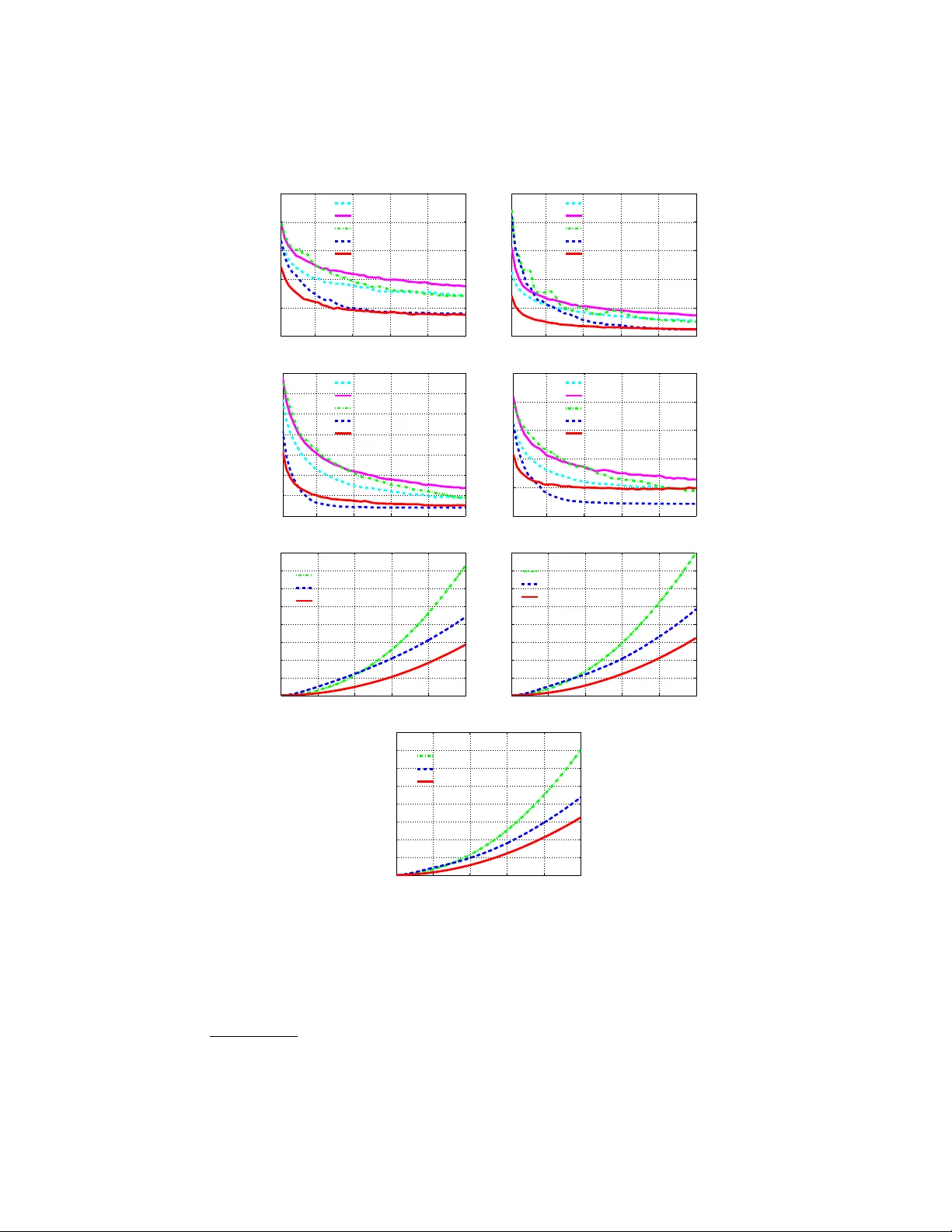
F ast T raining of Effectiv e Multi-class Bo osting Using Co ordinate Descen t Optimization ? Guosheng Lin, Ch unhua Shen ?? , An ton v an den Hengel, David Suter The Univ ersit y of Adelaide, Australia Abstract. W e presen t a nov el column generation based b oosting metho d for m ulti-class classification. Our multi-class bo osting is form ulated in a single optimization problem as in [1, 2]. Different from most existing m ulti-class b oosting metho ds, whic h use the same set of w eak learners for all the classes, w e train class specified weak learners (i.e., eac h class has a different set of w eak learners). W e show that using separate weak learner sets for each class leads to fast conv ergence, without in tro ducing additional computational ov erhead in the training pro cedure. T o further mak e the training more efficien t and scalable, w e also prop ose a fast co- ordinate descent metho d for solving the optimization problem at each b oosting iteration. The proposed coordinate descen t method is concep- tually simple and easy to implement in that it is a closed-form solution for eac h co ordinate update. Exp erimen tal results on a v ariety of datasets sho w that, compared to a range of existing multi-class bo osting meth- o ds, the prop osed metho d has muc h faster conv ergence rate and b etter generalization p erformance in most cases. W e also empirically sho w that the proposed fast co ordinate descent algorithm needs less training time than the MultiBo ost algorithm in Shen and Hao [1]. 1 In tro duction Bo osting metho ds combine a set of weak classifiers (w eak learners) to form a strong classifier. Bo osting has been extensiv ely studied [3, 4] and applied to a wide range of applications due to its robustness and efficiency (e.g., real-time ob ject detection [5–7]). Despite that fact that most classification tasks are inher- en tly m ulti-class problems, the ma jority of bo osting algorithms are designed for binary classification. A p opular approach to multi-class b o osting is to split the m ulti-class problem into a bunc h of binary classification problems. A simple ex- ample is the one-vs-all approach. The w ell-kno wn error correcting output co ding (ECOC) metho ds [8] belong to this category . AdaBo ost.ECC [9], AdaBo ost.MH [10] and AdaBo ost.MO [10] can all b e viewed as examples of the ECOC approac h. The second approac h is to directly form ulate m ulti-class as a single learning task, whic h is based on pairwise mo del comparisons b et ween different classes. Shen ? Co de can b e downloaded at http://goo.gl/WluhrQ . This pap er was published in Pro c. 11th Asian Conference on Computer Vision, Korea 2012. ?? Corresp onding author: chshhen@gmail.com . 2 G. Lin, C. Shen, A. v an den Hengel, D. Suter and Hao’s direct form ulation for m ulti-class b oosting (referred to as MultiBo ost) is such an example [1]. F rom the p ersp ectiv e of optimization, MultiBo ost can b e seen as an extension of the binary column generation b o osting framework [11, 4] to the multi-class case. Our w ork here builds up on MultiBo ost. As most existing m ulti-class b oosting, for MultiBo ost of [1], different classes share the same set of w eak learners, which leads to a sparse solution of the mo del parameters and hence slo w conv ergence. T o solve this problem, in this w ork we prop ose a no vel formu- lation (referred to as MultiBo ost cw ) for multi-class bo osting by using separate w eak learner sets. Namely , each class uses its own weak learner set. Compared to MultiBo ost, MultiBo ost cw con verges muc h faster, generally has b etter gener- alization p erformance and do es not in tro duce additional time cost for training. Note that AdaBo ost.MO prop osed in [10] uses different sets of weak classifiers for each class to o. AdaBo ost.MO is based on ECOC and the co de matrix in Ad- aBo ost.MO is specified b efore learning. Therefore, the underlying dep endence b et w een the fixed code matrix and generated binary classifiers is not explic- itly taken into consideration, compared with AdaBoost.ECC. In contrast, our MultiBo ost cw is based on the direct form ulation of multi-class b o osting, which leads to fundamentally different optimization strategies. More importantly , as sho wn in our exp erimen ts, our MultiBo ost cw is m uc h more scalable than Ad- aBo ost.MO although both enjoy faster conv ergence than most other multi-class b oosting. In MultiBoost [1], sophisticated optimization tools like Mosek or LBF GS-B [12] are needed to solv e the resulting optimization problem at each bo osting iter- ation, whic h is not v ery scalable. Here w e propose a co ordinate descen t algorithm (F CD) for fast optimization of the resulting problem at each bo osting iteration of MultiBo ost cw . FCD metho ds choose one v ariable at a time and efficiently solv e the single-v ariable sub-problem. CD(co ordinate decent) has b een applied to solv e many large-scale optimization problems. F or example, Y uan et al. [13] made comprehensiv e empirical comparisons of ` 1 regularized classification algo- rithms. They concluded that CD methods are very competitive for solving large- scale problems. In the form ulation of MultiBoost (also in our MultiBoost cw ), the n umber of v ariables is the pro duct of the n umber of classes and the num ber of w eak learners, whic h can b e very large (esp ecially when the num ber of classes is large). Therefore CD metho ds may b e a b etter choice for fast optimization of m ulti-class bo osting. Our method F CD is sp ecially tailored for the optimization of MultiBo ost cw . W e are able to obtain a closed-form solution for each v ariable up date. Th us the optimization can b e extremely fast. The proposed FCD is easy to implemen t and no sophisticated optimization to olb o x is required. Main Contributions 1) W e prop ose a nov el multi-class b o osting metho d (MultiBo ost cw ) that uses class sp ecified weak learners. Unlik e MultiBo ost shar- ing a single set of weak learners across different classes, our metho d uses a separate set of weak learners for each class. W e generate K (the num b er of classes) weak learners in each b oosting iteration—one weak learner for each class. With this mechanism, w e are able to ac hieve muc h faster conv ergence. 2) Similar to MultiBo ost [1], w e emplo y column generation to implemen t the F ast T raining of Multi-class Bo osting 3 b oosting training. W e derive the Lagrange dual problem of the new multi-class b oosting form ulation which enable us to design fully corrective multi-class al- gorithms using the primal-dual optimization technique. 3) W e prop ose a F CD metho d for fast training of MultiBo ost cw . W e obtain an analytical solution for eac h v ariable update in co ordinate descent. W e use the Karush-Kuhn-T uc ker (KKT) conditions to deriv e effective stop criteria and construct w orking sets of violated v ariables for faster optimization. W e show that FCD can be applied to fully corrective optimization (up dating all v ariables) in m ulti-class bo osting, similar to fast stage-wise optimization in standard AdaBo ost (up dating newly added v ariables only). Notation Let us as sume that we hav e K classes. A weak learner is a func- tion that maps an example x to {− 1 , +1 } . W e denote each weak learner by ~ : ~ y ,j ( · , · ) ∈ F , ( y = 1 . . . K , and j = 1 . . . n ). F is the space of all the weak learners; n is the num b er of weak learners. W e define column vectors h y ( x ) = [ ~ y , 1 ( x ) , · · · , ~ y ,n ( x )] > as the outputs of weak learners asso ciated with the y -th class on example x . Let us denote the weak learners’ co efficien ts w y for class y . Then the strong classifier for class y is F y ( x ) = w > h y ( x ). W e need to learn K strong classifiers, one for each class. Giv en a test data x , the classification rule is y ? = argmax F y ( x ). 1 is a vector with elemen ts all b eing one. Its dimension should b e clear from the context. 2 Our Approach W e show how to formulate the multi-class b oosting problem in the large mar- gin learning framework. Analogue to MultiBo ost, we can define the multi-class margins asso ciate with training data ( x i , y i ) as γ ( i,y ) = w > y i h y i ( x i ) − w > y h y ( x i ) , (1) for y 6 = y i . In tuitively , γ ( i,y ) is the difference of the classification scores b et ween a “wrong” model and the right mo del. W e w ant to mak e this margin as large as p ossible. MultiBo ost cw with the exp onen tial loss can b e formulated as: min w ≥ 0 , γ k w k 1 + C p X i X y 6 = y i exp( − γ ( i,y ) ) , ∀ i = 1 · · · m ; ∀ y ∈ { 1 · · · K }\ y i . (2) Here γ is defined in (1). W e hav e also introduced a shorthand symbol p = m × ( K − 1). The parameter C controls the complexity of the learned model. The mo del parameter is w = [ w 1 ; w 2 ; . . . , w K ] > ∈ R K · n × 1 . Minimizing (2) encourages the confidence score of the correct lab el y i of a training example x i to b e larger than the confidence of other lab els. W e de- fine Y as a set of K lab els: Y = { 1 , 2 , . . . , K } . The discriminant function F : X × Y 7→ R we need to learn is: F ( x , y ; w ) = w > y h y ( x ) = P j w ( y ,j ) ~ ( y ,j ) ( x ). The class lab el prediction y ? for an unknown example x is to maximize F ( x , y ; w ) o ver y , which means finding a class lab el with the largest confidence: y ? = 4 G. Lin, C. Shen, A. v an den Hengel, D. Suter Algorithm 1 CG: Column generation for MultiBo ost cw 1: Input: training examples ( x 1 ; y 1 ) , ( x 2 ; y 2 ) , · · · ; regularization parameter C ; termi- nation threshold and the maximum iteration num ber. 2: Initialize: W orking weak learner set H c = ∅ ( c = 1 · · · K ); initialize ∀ ( i, y 6 = y i ) : λ ( i,y ) = 1 ( i = 1 , . . . , m, y = 1 , . . . , K ). 3: Rep eat 4: − Solve (4) to find K w eak learners: ~ ? c ( · ) , c = 1 · · · K ; and add them to the w orking w eak learner set H c . 5: − Solve the primal problem (2) on the curren t working weak learner sets: ~ c ∈ H c , c = 1 , . . . , K . to obtain w (we use co ordinate descent of Algorithm 2). 6: − Update dual v ariables λ in (5) using the primal solution w and the KKT con- ditions (5). 7: Until the relativ e change of the primal ob jectiv e function v alue is smaller than the prescrib ed tolerance; or the maxim um iteration is reached. 8: Output: K discriminan t function F ( x , y ; w ) = w > y h y ( x ), y = 1 · · · K . argmax y F ( x , y ; w ) = argmax y w > y h ( x ) . MultiBoost cw is an extension of Multi- Bo ost [1] for m ulti-class classification. The only difference is that, in MultiBoost, differen t classes share the same set of weak learners h . In contrast, each class asso ciates a separate set of weak learners. W e show that MultiBo ost cw learns a more compact mo del than MultiBo ost. Column generation for MultiBo ost cw T o implement b oosting, we need to derive the dual problem of (2). Similar to [1], the dual problem of (2) can be written as (3), in whic h c is the index of class lab els. λ ( i,y ) is the dual v ariable asso ciated with one constraint in (2): max λ X i X y 6 = y i λ ( i,y )  1 − log p C − log λ ( i,y )  (3a) s . t . ∀ c = 1 , . . . , K : X i ( y i = c ) X y 6 = y i λ ( i,y ) h y i ( x i ) − X i X y 6 = y i ,y = c λ ( i,y ) h y ( x i ) ≤ 1 , (3b) ∀ i = 1 , . . . , m : 0 ≤ X y 6 = y i λ ( i,y ) ≤ C p . (3c) F ollo wing the idea of column generation [4], we divide the original problem (2) in to a master problem and a sub-problem, and solve them alternativ ely . The master problem is a restricted problem of (2) whic h only considers the generated w eak learners. The sub-problem is to generate K w eak learners (corresp onding K classes) by finding the most violated constraint of eac h class in the dual form (3), and add them to the master problem at each iteration. The sub-problem for F ast T raining of Multi-class Bo osting 5 finding most violated constrain ts can b e written as: ∀ i =1 · · · K : ~ ? c ( · ) = argmax ~ c ( · ) X i ( y i = c ) X y 6 = y i λ ( i,y ) h y i ( x i ) − X i X y 6 = y i ,y = c λ ( i,y ) h y ( x i ) . (4) The column generation pro cedure for MultiBo ost cw is describ ed in Algorithm 1. Essen tially , we rep eat the follo wing tw o steps until conv ergence: 1) W e solve the master problem (2) with ~ c ∈ H c , c = 1 , . . . , K , to obtain the primal solution w . H c is the w orking set of generated weak learners asso ciated with the c -th class. W e obtain the dual solution λ ? from the primal solution w ? using the KKT conditions: λ ? ( i,y ) = C p exp  w ? > y h y ( x i ) − w ? > y i h y i ( x i )  . (5) 2) With the dual solution λ ? ( i,y ) , w e solv e the sub-problem (4) to generate K w eak learners: ~ ? c , c = 1 , 2 , . . . , K , and add to the working weak learner set H c . In MultiBoost cw , K weak learners are generated for K classes respectively in eac h iteration, while in MultiBoost, only one weak learner is generated at each column generation and shared by all classes. As shown in [1] for MultiBo ost, the sub-problem for finding the most violated constrain t in the dual form is: [ ~ ? ( · ) , c ? ] = argmax ~ ( · ) , c X i ( y i = c ) X y 6 = y i λ ( i,y ) h ( x i ) − X i X y 6 = y i ,y = c λ ( i,y ) h ( x i ) . (6) A t eac h column generation of MultiBo ost, (6) is solved to generated one weak learner. Note that solving (6) is to search ov er al l K classes to find the b est w eak learner ~ ? . Thus the computational cost is the same as MultiBo ost cw . This is the reason why MultiBo ost cw do es not introduce additional training cost compared to MultiBo ost. In general, the solution [ w 1 ; · · · ; w K ] of MultiBo ost is highly sparse [1]. This can b e observed in our empirical study . The w eak learner generated by solving (6) actually is targeted for one class, th us using this w eak learner across all classes in MultiBo ost leads to a very sparse solution. The sparsit y of [ w 1 , · · · , w K ] indicates that one weak learner is usually only useful for the prediction of a very few n um b er of classes (t ypically only one), but useless for most other classes. In this sense, forcing different classes to use the same set of weak learners may not b e necessary and usually it leads to slow conv ergence. In con trast, using separate w eak learner sets for eac h class, MultiBo ost cw tends to ha ve a dense solution of w . With K w eak learners generated at eac h iteration, MultiBo ost cw con verges m uch faster. F ast co ordinate descen t T o further sp eed up the training, we prop ose a fast co ordinate descen t metho d (FCD) for solving the primal MultiBoost cw problem at each column generation iteration. The details of FCD is presented in Algorithm 2. The high-level idea is simple. F CD works iterativ ely , and at eac h iteration (working set iteration), we compute the violated v alue of the KKT conditions for each v ariable in w , and construct a w orking set of violated 6 G. Lin, C. Shen, A. v an den Hengel, D. Suter v ariables (denoted as S ), then pick v ariables from the S for update (one v ariable at a time). W e also use the violated v alues for defining stop criteria. Our FCD is a mix of sequential and sto c hastic co ordinate descent. F or the first working set iteration, v ariables are sequentially pic ked for update (cyclic CD); in later w orking set iterations, v ariables are randomly pic ked (stochastic CD). In the sequel, we present the details of F CD. First, we describe ho w to up date one v ariable of w by solving a single-v ariable sub-problem. F or notation simplicity , w e define: δ h i ( y ) = h y i ( x i ) ⊗ Γ ( y i ) − h y ( x i ) ⊗ Γ ( y ) . Γ ( y ) is the orthogonal label co ding vector: Γ ( y ) = [ δ ( y, 1) , δ ( y , 2) , · · · , δ ( y , K )] > ∈ { 0 , 1 } K . Here δ ( y, k ) is the indicator function that returns 1 if y = k , otherwise 0. ⊗ denotes the tensor pro duct. MultiBo ost cw in (2) can b e equiv alently written as: min w ≥ 0 k w k 1 + C p X i X y 6 = y i exp  − w > δ h i ( y )  . (7) W e assume that binary w eak learners are used here: ~ ( x ) ∈ { +1 , − 1 } . δ h i,j ( y ) denotes the j -th dimension of δ h i ( y ), and δ ˆ h i,j ( y ) denotes the rest dimensions of δ h i ( y ) excluding the j -th. The output of δ h i,j ( y ) only takes three p ossi- ble v alues: δ h i,j ( y ) ∈ {− 1 , 0 , +1 } . F or the j -th dimension, we define: D j v = { ( i, y ) | δ h j i ( y ) = v , i ∈ { 1 , . . . , m } , y ∈ Y /y i } , v ∈ {− 1 , 0 , +1 } ; so D j v is a set of constraint indices ( i, y ) that the output of δ h i,j ( y ) is v . w j denotes the j -th v ariable of w ; ˆ w j denotes the rest v ariables of w excluding the j -th. Let g ( w ) b e the ob jective function of the optimization (7). g ( w ) can b e de-comp osited as: g ( w ) = k w k 1 + C p X i X y 6 = y i exp  − w > δ h i ( y )  = k ˆ w j k 1 + k w j k 1 + C p X i,y 6 = y i exp  − ˆ w > j δ ˆ h i,j ( y ) − w > j δ h i,j ( y )  = k ˆ w j k 1 + k w j k 1 + C p  exp( w > j ) X ( i,y ) ∈ D j − 1 exp  − ˆ w > j δ ˆ h i,j ( y )  + exp( − w > j ) X ( i,y ) ∈ D j +1 exp  − ˆ w > j δ ˆ h i,j ( y )  + X ( i,y ) ∈ D j 0 exp  − ˆ w > j δ ˆ h i,j ( y )   = k ˆ w j k 1 + k w j k 1 + C p  exp( w > j ) V − + exp( − w > j ) V + + V 0  . (8) Here w e hav e defined: V − = X ( i,y ) ∈ D j − 1 exp  − ˆ w > j δ ˆ h i,j ( y )  , V 0 = X ( i,y ) ∈ D j 0 exp  − ˆ w > j δ ˆ h i,j ( y )  , (9a) V + = X ( i,y ) ∈ D j +1 exp  − ˆ w > j δ ˆ h i,j ( y )  . (9b) In the v ariable up date step, one v ariable w j is pick ed at a time for up dating and other v ariables ˆ w j are fixed; thus we need to minimize g in (8) w.r.t w j , which F ast T raining of Multi-class Bo osting 7 is a single-v ariable minimization. It can b e written as: min w j ≥ 0 k w j k 1 + C p  V − exp( w > j ) + V + exp( − w > j )  . (10) The deriv ative of the ob jective function in (10) with w j > 0 is: ∂ g ∂ w j = 0 = ⇒ 1 + C p  V − exp( w > j ) − V + exp( − w > j )  = 0 . (11) By solving (11) and the b ounded constraint w j ≥ 0, we obtain the analytical solution of the optimization in (10) (since V − > 0): w ? j = max  0 , log  q V + V − + p 2 4 C 2 − p 2 C  − log V −  . (12) When C is large, (12) can b e appro ximately simplified as: w ? j = max  0 , 1 2 log V + V −  . (13) With the analytical solution in (12), the up date of each dimension of w can b e p erformed extremely efficiently . The main requirement for obtaining the closed- form solution is that the use of discrete weak learners. W e use the KKT conditions to construct a set of violated v ariables and de- riv e meaningful stop criteria. F or the optimization of MultiBo ost cw (7), KKT conditions are necessary conditions and also sufficient for optimality . The La- grangian of (7) is: L = k w k 1 + C p P i P y 6 = y i exp  − w > δ h i ( y )  − α > w . According to the KKT conditions, w ? is the optimal for (10) if and only if w ? satisfies w ? ≥ 0 , α ? ≥ 0 , ∀ j : α ? j w ? j = 0 and ∀ j : ∇ j L ( w ? ) = 0. F or w j > 0, ∂ L ∂ w j = 0 = ⇒ 1 − C p X i X y 6 = y i exp  − w δ h i ( y )  δ h i,j ( y ) − α j = 0 . Considering the complementary slackness: α ? j w ? j = 0, if w ? j > 0, w e hav e α ? j = 0; if w ? j = 0, w e hav e α ? j ≥ 0. The optimality conditions can be written as: ∀ j : ( 1 − C p P i P y 6 = y i exp  − w ? δ h i ( y )  δ h i,j ( y ) = 0 , if w ? j > 0; 1 − C p P i P y 6 = y i exp  − w ? δ h i ( y )  δ h i,j ( y ) ≥ 0 , if w ? j = 0 . (14) F or notation simplicity , we define a column v ector µ as in (15). With the op- timalit y conditions (14), we define θ j in (16) as the violated v alue of the j -th v ariable of the solution w ? : µ ( i,y ) = exp  − w > δ h i ( y )  (15) θ j = ( | 1 − C p P i P y 6 = y i µ ( i,y ) δ h i,j ( y ) | if w ? j > 0 max { 0 , C p P i P y 6 = y i µ ( i,y ) δ h i,j ( y ) − 1 } if w ? j = 0 . (16) 8 G. Lin, C. Shen, A. v an den Hengel, D. Suter A t eac h working set iteration of F CD, we compute the violated v alues θ , and construct a working set S of violated v ariables; then we randomly (except the first iteration) pick one v ariable from S for up date. W e rep eat picking for | S | times; | S | is the elemen t num b er of S . S is defined as S = { j | θ j >  } (17) where  is a tolerance parameter. Analogue to [14] and [13], with the definition of the v ariable violated v alues θ in (16), we can define the stop criteria as: max j θ j ≤ , (18) where  can b e the same tolerance parameter as in the w orking set S definition (17). The stop condition (18) shows if the largest violated v alue is smaller than some threshold, F CD terminates. W e can see that using KKT conditions is actually using the gradient information. An inexact solution for w is acceptable for each column generation iteration, th us w e place a maxim um iteration n umber ( τ max in Algorithm 2) for F CD to preven t unnecessary computation. W e need to compute µ b efore obtaining θ , but computing µ in (15) is exp ensiv e. F ortunately , w e are able to efficien tly up date µ after the up date of one v ariable w j to av oid re-computing of (15). µ in (15) can b e equally written as: µ ( i,y ) = exp  − ˆ w > j δ ˆ h i,j ( y ) − w j δ h i,j ( y )  . (19) So the up date of µ is then: µ ( i,y ) = µ old ( i,y ) exp  δ h i,j ( y )( w old j − w j )  . (20) With the definition of µ in (19), the v alues V − and V + for one v ariable up date can b e efficiently computed by using µ to av oid the exp ensiv e computation in (9a) and (9b); V − and V + can b e equally defined as: V − = X ( i,y ) ∈ D j − 1 µ ( i,y ) exp( − w j ) , V + = X ( i,y ) ∈ D j +1 µ ( i,y ) exp( w j ) . (21) Some discussion on FCD (Algorithm 2) is as follows: 1) Stage-wise optimiza- tion is a sp ecial case of FCD. Compared to totally corrective optimization which considers all v ariables of w for up date, stage-wise only considers those newly added v ariables for up date. W e initialize the w orking set using the newly added v ariables. F or the first working set iteration, w e sequen tially up date the new added v ariables. If setting the maximum working set iteration to 1 ( τ max = 1 in Algorithm 2), FCD b ecomes a stage-wise algorithm. Thus FCD is a general- ized algorithm with totally corrective up date and stage-wise up date as sp ecial cases. In the stage-wise setting, usually a large C (regularization parameter) is implicitly enforced, thus we can use the analytical solution in (13) for v ariable up date. 2) Randomly picking one v ariable for up date without an y guidance leads to slo w lo cal conv ergence. When the solution gets close to the optimality , usually F ast T raining of Multi-class Bo osting 9 Algorithm 2 FCD: F ast coordinate decen t for MultiBoost cw 1: Input: training examples ( x 1 ; y 1 ) , · · · , ( x m ; y m ); parameter C ; tolerance:  ; weak learner set H c , c = 1 , . . . , K ; initial v alue of w ; maxim um w orking set iteration: τ max . 2: Initialize: initialize v ariable working set S b y v ariable indices in w that corresp ond to newly added w eak learners; initialize µ in (15); working set iteration index τ = 0. 3: Rep eat (working set iteration) 4: τ = τ + 1; reset the inner lo op index: q = 0; 5: While q < | S | ( | S | is the size of S ) 6: q = q + 1; pic k one v ariable index j from S : if τ = 1 sequentially pic k one, else randomly pic k one. 7: Compute V − and V + in (21) using µ . 8: up date v ariable w j in (12) using V − and V + . 9: up date µ in (20) using the up dated w j . 10: End While 11: Compute the violated v alues θ in (16) for all v ariables. 12: Re-construct the v ariable w orking set S in (17) using θ . 13: Un til the stop condition in (18) is satisfied or maxim um w orking set iteration reac hed: τ > = τ max . 14: Output: w . only very few v ariables need up date, and most pic ks do not “hit”. In column generation (CG), the initial v alue of w is initialized b y the solution of last CG iteration. This initialization is already fairly close to optimalit y . Therefore the slo w lo cal con vergence for sto chastic coordinate decent (CD) is more serious in column generation based bo osting. Here we hav e used the KKT conditions to iterativ ely construct a working set of violated v ariables, and only the v ariables in the w orking set need up date. This strategy leads to faster CD conv ergence. 3 Exp erimen ts W e ev aluate our metho d MultiBo ost cw on some UCI datasets and a v ariety of multi-class image classification applications, including digit recognition, scene recognition, and traffic sign recognition. W e compare MultiBo ost cw against Multi- Bo ost [1] with the exp onen tial loss, and another there popular multi-class b oost- ing algorithms: AdaBo ost.ECC [9], AdaBo ost.MH [10] and AdaBoost.MO [10]. W e use FCD as the solv er for MultiBo ost cw , and LBFGS-B [12] for MultiBoost. W e also perform further experiments to ev aluate FCD in detail. F or all exp eri- men ts, the b est regularization parameter C for MultiBo ost cw and MultiBo ost is selected from 10 2 to 10 5 ; the tolerance parameter in FCD is set to 0 . 1 (  = 0 . 1); W e use MultiBo ost cw -1 to denote MultiBoost cw using the stage-wise setting of F CD which only uses one iteration ( τ max = 1 in Algorithm 2). In MultiBo ost cw - 1, w e fix C to b e a large v alue: C = 10 8 . All exp eriments are run 5 times. W e compare the testing error, the total train- ing time and solv er time on all datasets. The results sho w that our MultiBoost cw and MultiBoost cw -1 con verge muc h faster then other metho ds, use less training time then MultiBo ost, and achiev e the b est testing error on most datasets. 10 G. Lin, C. Shen, A. v an den Hengel, D. Suter 100 200 300 400 500 0 0.1 0.2 0.3 0.4 0.5 0.6 0.7 0.8 iterations [VOWEL] Test error ADA.MO(0.117 ± 0.014) ADA.MH(0.130 ± 0.016) ADA.ECC(0.103 ± 0.024) MultiB(0.080 ± 0.025) CW(ours)(0.101 ± 0.016) CW−1(ours)(0.085 ± 0.018) 100 200 300 400 500 0 100 200 300 400 500 iterations [VOWEL] Training time (seconds) ADA.MO (419.7 ± 39.5) MultiB (135.5 ± 10.4) CW(ours) (107.5 ± 7.2) CW−1(ours) (76.8 ± 4.8) 100 200 300 400 500 0 10 20 30 40 50 60 70 iterations [VOWEL] Solver time (seconds) MultiB (69.6 ± 5.4) CW(ours) (43.5 ± 4.0) CW−1(ours) (24.7 ± 1.7) 100 200 300 400 500 0 0.2 0.4 0.6 0.8 1 iterations [ISOLET] Test error ADA.MH(0.067 ± 0.005) ADA.ECC(0.106 ± 0.008) MultiB(0.069 ± 0.005) CW(ours)(0.056 ± 0.007) CW−1(ours)(0.050 ± 0.004) 100 200 300 400 500 0 500 1000 1500 2000 2500 3000 3500 4000 iterations [ISOLET] Training time (seconds) MultiB (3621.3 ± 549.8) CW(ours) (2430.4 ± 371.1) CW−1(ours) (2553.8 ± 213.8) 100 200 300 400 500 0 500 1000 1500 2000 iterations [ISOLET] Solver time (seconds) MultiB (1604.7 ± 243.8) CW(ours) (746.7 ± 119.5) CW−1(ours) (699.7 ± 58.8) Fig. 1: Results of 2 UCI datasets: VO WEL and ISOLET. CW and CW-1 are our metho ds. CW-1 uses stage-wise setting. The n umber after the method name is the mean v alue with standard deviation of the last iteration. Our methods conv erge muc h faster and achiev e comp etitiv e test accuracy . The total training time and the solver time of our methods both are less than MultiBoost of [1]. AdaBo ost.MO [10] (Ada.MO) has a similar conv ergence rate as our metho d, but it is muc h slo wer than our me thod and b ecomes in tractable for large scale datasets. W e run Ada.MO on some UCI datasets and MNIST. Results are sho wn in Fig. 1 and Fig. 2. W e set a maxim um training time (1000 seconds) for Ada.MO; other metho ds are all b elo w this maximum time on those datasets. If maxim um time reac hed, we report the results of those finished iterations. UCI datasets : w e use 2 UCI multi-class datasets: VO WEL and ISOLET. F or each dataset, w e randomly select 75% data for training and the rest for testing. Results are sho wn in Fig. 1. Handwritten digit recognition : we use 3 handwritten datasets: MNIST, USPS and PENDIGITS. F or MNIST, we randomly sample 1000 examples from eac h class, and use the original test set of 10,000 examples. F or USPS and PENDIGITS, we randomly select 75% for training, the rest for testing. Results are sho wn in Fig. 2. 3 Image datasets: P ASCAL07, Lab elMe, CIF AR10 : F or P ASCAL07, w e use 5 types of features pro vided in [15]. F or labelMe, we use the subset: Lab elMe-12-50k 1 and generate GIST features. F or these t wo datasets, we use those images whic h only hav e one class lab el. W e use 70% data for training, the rest for testing. F or CIF AR10 2 , we construct 2 datasets, one uses GIST features 1 h ttp://www.ais.uni-b onn.de/do wnload/datasets.html 2 h ttp://www.cs.toronto.edu/˜kriz/cifar.h tml F ast T raining of Multi-class Bo osting 11 100 200 300 400 500 0 0.1 0.2 0.3 0.4 0.5 0.6 0.7 iterations [USPS] Test error ADA.MO(0.057 ± 0.006) ADA.MH(0.056 ± 0.003) ADA.ECC(0.061 ± 0.007) MultiB(0.053 ± 0.004) CW(ours)(0.046 ± 0.001) CW−1(ours)(0.042 ± 0.002) 100 200 300 400 500 0 200 400 600 800 1000 iterations [USPS] Training time (seconds) ADA.MO (990.8 ± 8.8) MultiB (847.1 ± 126.5) CW(ours) (518.4 ± 86.5) CW−1(ours) (394.3 ± 7.5) 100 200 300 400 500 0 100 200 300 400 500 iterations [USPS] Solver time (seconds) MultiB (408.1 ± 69.9) CW(ours) (188.4 ± 36.0) CW−1(ours) (110.8 ± 2.5) 100 200 300 400 500 0 0.1 0.2 0.3 0.4 0.5 iterations [PENDIGITS] Test error ADA.MO(0.042 ± 0.004) ADA.MH(0.035 ± 0.003) ADA.ECC(0.035 ± 0.003) MultiB(0.022 ± 0.001) CW(ours)(0.023 ± 0.003) CW−1(ours)(0.019 ± 0.003) 100 200 300 400 500 0 200 400 600 800 1000 iterations [PENDIGITS] Training time (seconds) ADA.MO (976.7 ± 25.0) MultiB (936.5 ± 153.1) CW(ours) (592.9 ± 96.3) CW−1(ours) (404.9 ± 2.9) 100 200 300 400 500 0 100 200 300 400 500 iterations [PENDIGITS] Solver time (seconds) MultiB (477.6 ± 80.2) CW(ours) (238.8 ± 34.3) CW−1(ours) (121.6 ± 1.5) 100 200 300 400 500 0 0.1 0.2 0.3 0.4 0.5 0.6 0.7 iterations [MNIST] Test error ADA.MO(0.110 ± 0.001) ADA.MH(0.109 ± 0.002) ADA.ECC(0.121 ± 0.003) MultiB(0.104 ± 0.004) CW(ours)(0.097 ± 0.004) CW−1(ours)(0.092 ± 0.001) 100 200 300 400 500 0 200 400 600 800 1000 iterations [MNIST] Training time (seconds) ADA.MO (981.3 ± 14.6) MultiB (956.5 ± 56.8) CW(ours) (730.1 ± 99.3) CW−1(ours) (577.6 ± 5.9) 100 200 300 400 500 0 100 200 300 400 500 iterations [MNIST] Solver time (seconds) MultiB (468.4 ± 18.3) CW(ours) (255.7 ± 27.4) CW−1(ours) (163.6 ± 3.2) Fig. 2: Exp eriments on 3 handwritten digit recognition datasets: USPS, PENDIGITS and MNIST. CW and CW-1 are our metho ds. CW-1 uses stage-wise setting. Our meth- o ds conv erge m uch faster, achiev e b est test error and use less training time. Ada.MO has similar con vergence rate as ours, but requires muc h more training time. With a maxim um training time of 1000 seconds, Ada.MO failed to finish 500 iterations on all 3 datasets. and the other uses the pixel v alues. W e use the provided test set and 5 training sets for 5 times run. Results are shown in Fig. 3. Scene recognition : we use 2 scene image datasets: Scene15 [16] and SUN [17]. F or Scene15, w e randomly select 100 images p er class for training, and the rest for testing. W e generate histograms of co de words as features. The code b ook size is 200. An image is divided in to 31 sub-windo ws in a spatial hierarch y manner. W e generate histograms in each sub-windows, so the histogram feature dimension is 6200. F or SUN dataset, w e construct a subset of the original dataset con taining 25 categories. F or eac h category , we use the top 200 images, and randomly select 80% data for training, the rest for testing. W e use the HOG features describ ed in[17]. Results are shown in Fig. 4. 12 G. Lin, C. Shen, A. v an den Hengel, D. Suter 100 200 300 400 500 0.4 0.5 0.6 0.7 0.8 0.9 iterations [PASCAL07] Test error ADA.MH(0.545 ± 0.008) ADA.ECC(0.575 ± 0.008) MultiB(0.541 ± 0.007) CW(ours)(0.480 ± 0.003) CW−1(ours)(0.475 ± 0.003) 100 200 300 400 500 0.2 0.3 0.4 0.5 0.6 0.7 iterations [LABELME−SUB] Test error ADA.MH(0.254 ± 0.002) ADA.ECC(0.273 ± 0.004) MultiB(0.250 ± 0.004) CW(ours)(0.223 ± 0.002) CW−1(ours)(0.225 ± 0.002) 100 200 300 400 500 0.45 0.5 0.55 0.6 0.65 0.7 0.75 0.8 iterations [CIFAR10−GIST] Test error ADA.MH(0.495 ± 0.006) ADA.ECC(0.518 ± 0.005) MultiB(0.495 ± 0.004) CW(ours)(0.470 ± 0.002) CW−1(ours)(0.476 ± 0.004) 100 200 300 400 500 0.65 0.7 0.75 0.8 0.85 iterations [CIFAR10−RAW] Test error ADA.MH(0.647 ± 0.004) ADA.ECC(0.664 ± 0.003) MultiB(0.644 ± 0.006) CW(ours)(0.621 ± 0.004) CW−1(ours)(0.648 ± 0.004) 100 200 300 400 500 0 100 200 300 400 500 600 700 800 iterations [PASCAL07] Solver time (seconds) MultiB (728.6 ± 71.9) CW(ours) (440.7 ± 33.5) CW−1(ours) (285.4 ± 2.4) 100 200 300 400 500 0 50 100 150 200 250 300 350 400 iterations [CIFAR10−RAW] Solver time (seconds) MultiB (400.0 ± 39.4) CW(ours) (242.0 ± 35.4) CW−1(ours) (161.6 ± 2.0) 100 200 300 400 500 0 50 100 150 200 250 300 350 400 iterations [CIFAR10−GIST] Solver time (seconds) MultiB (350.9 ± 37.5) CW(ours) (218.2 ± 20.0) CW−1(ours) (161.9 ± 4.5) Fig. 3: Exp eriments on 3 image datasets: P ASCAL07, Lab elMe and CIF AR10. CW and CW-1 are our metho ds. CW-1 uses stage-wise setting. Our metho ds con verge muc h faster, achiev e b est test error and use less training time. T raffic sign recognition : W e use the GTSRB 3 traffic sign dataset. There are 43 classes and more than 50000 images. W e use the pro vided 3 types of HOG 3 h ttp://b enc hmark.ini.rub.de/ F ast T raining of Multi-class Bo osting 13 100 200 300 400 500 0.2 0.3 0.4 0.5 0.6 0.7 0.8 0.9 1 iterations [SCENE15] Test error ADA.MH(0.245 ± 0.009) ADA.ECC(0.269 ± 0.005) MultiB(0.278 ± 0.004) CW(ours)(0.229 ± 0.004) CW−1(ours)(0.225 ± 0.005) 100 200 300 400 500 0 100 200 300 400 500 600 iterations [SCENE15] Training time (seconds) MultiB (592.1 ± 52.6) CW(ours) (417.1 ± 25.6) CW−1(ours) (278.5 ± 6.2) 100 200 300 400 500 0 50 100 150 200 250 iterations [SCENE15] Solver time (seconds) MultiB (242.0 ± 25.0) CW(ours) (103.7 ± 10.1) CW−1(ours) (49.5 ± 0.9) 100 200 300 400 500 0.5 0.55 0.6 0.65 0.7 0.75 0.8 0.85 0.9 iterations [SUN−25] Test error ADA.MH(0.564 ± 0.013) ADA.ECC(0.606 ± 0.013) MultiB(0.601 ± 0.008) CW(ours)(0.525 ± 0.009) CW−1(ours)(0.528 ± 0.007) 100 200 300 400 500 0 500 1000 1500 2000 2500 iterations [SUN−25] Training time (seconds) MultiB (2189.6 ± 85.4) CW(ours) (1850.2 ± 47.0) CW−1(ours) (1589.1 ± 51.9) 100 200 300 400 500 0 200 400 600 800 1000 iterations [SUN−25] Solver time (seconds) MultiB (944.3 ± 46.3) CW(ours) (541.8 ± 19.6) CW−1(ours) (340.1 ± 20.2) Fig. 4: Exp erimen ts on 2 scene recognition datasets: SCENE15 and a subset of SUN. CW and CW-1 are our methods. CW-1 uses stage-wise setting. Our metho ds conv erge m uch faster and ac hieve best test error and use less training time. features; so there are 6052 features in total. W e randomly select 100 examples p er class for training and use the original test set. Results are shown in Fig.5. 3.1 F CD ev aluation W e perform further exp erimen ts to ev aluate F CD with differen t parameter set- tings, and compare to the LBF GS-B [12] solv er. W e use 3 datasets in this section: V OWEL, USPS and SCENE15. W e run FCD with different settings of the max- im um w orking set iteration( τ max in Algorithm 2) to ev aluate how the setting of τ max (maxim um working set iteration) affects the p erformance of FCD. W e also run LBF GS-B [12] solver for solving the same optimization (2) as F CD. W e set C = 10 4 for all cases. Results are sho wn in Fig. 6. F or LBFGS-B, we use the default conv erge setting to get a mo derate solution. The num b er after “FCD” in the figure is the setting of τ max in Algorithm 2 for FCD. Results show that the stage-wise case ( τ max = 1) of F CD is the fastest one, as exp ected. When we set τ max ≥ 2, the ob jective v alue of the optimization (2) of our metho d con verges m uch faster than LBFGS-B. Thus setting of τ max = 2 is sufficien t to achiev e a v ery accurate solution, and at the same time has faster con vergence and less running time than LBF GS-B. 4 Conclusion In this w ork, we hav e presented a nov el multi-class b oosting metho d. Based on the dual problem, b oosting is implemen ted using the column generation tec h- 14 G. Lin, C. Shen, A. v an den Hengel, D. Suter 50 100 150 200 0 0.2 0.4 0.6 0.8 1 iterations [GTSRB] Test error ADA.MH(0.103 ± 0.005) ADA.ECC(0.236 ± 0.011) MultiB(0.116 ± 0.008) CW(ours)(0.081 ± 0.004) CW−1(ours)(0.082 ± 0.003) 50 100 150 200 0 50 100 150 200 250 300 350 400 iterations [GTSRB] Solver time (seconds) MultiB (380.1 ± 6.0) CW(ours) (260.0 ± 9.0) CW−1(ours) (205.7 ± 9.4) Fig. 5: Results on the traffic sign dataset: GTSRB. CW and CW-1 (stage-wise setting) are our methods. Our metho ds conv erge muc h faster, ac hieve best test error and use less training time. nique. Different from most existing multi-class b oosting, we train a weak learner set for eac h class, which results in m uch faster conv ergence. A wide range of exp erimen ts on a few different datasets demonstrate that the prop osed multi-class bo osting achiev es comp etitiv e test accuracy compared with other existing multi-class b oosting. Y et it conv erges muc h faster and due to the prop osed efficient co ordinate descent metho d, the training of our method is m uch faster than the coun terpart of MultiBo ost in [1]. Ac knowledgemen t . This work w as supported b y ARC grants LP120200485 and FT120100969. References 1. Shen, C., Hao, Z.: A direct form ulation for totally-corrective multi-class b o osting. In: Pro c. IEEE Conf. Comp. Vis. Patt. Recogn. (2011) 2. P aisitkriangkrai, S., Shen, C., v an den Hengel, A.: Sharing features in multi-class b oosting via group sparsit y . In: Pro c. IEEE Conf. Comp. Vis. P att. Recogn. (2012) 3. Sc hapire, R.E., F reund, Y., Bartlett, P ., Lee, W.S.: b o osting the margin: A new explanation for the effectiv eness of voting metho ds. Annals of Statistics 26 (1998) 1651–1686 4. Shen, C., Li, H.: On the dual formulation of b oosting algorithms. IEEE T rans. P attern Anal. Mach. In tell. 32 (2010) 2216–2231 5. Viola, P ., Jones, M.J.: Robust real-time face detection. In t. J. Comput. Vision 57 (2004) 137–154 6. W ang, P ., Shen, C., Barnes, N., Zheng, H.: F ast and robust ob ject detection using asymmetric totally-corrective bo osting. IEEE T rans. Neural Netw orks & Learn. Syst. 23 (2012) 33–46 7. P aisitkriangkrai, S., Shen, C., Zhang, J.: F ast p edestrian detection using a cascade of b oosted cov ariance features. IEEE T rans. Circuits & Syst. for Video T ech. 18 (2008) 1140–1151 8. Dietteric h, T.G., Bakiri, G.: Solving m ulticlass learning problems via error- correcting output co des. J. Artif. Int. Res. 2 (1995) 263–286 F ast T raining of Multi-class Bo osting 15 50 100 150 200 250 300 400 600 800 1000 1200 1400 1600 boosting iterations [VOWEL] Objective function value LBFGS−B (357.297 ± 6.773) FCD−10 (337.756 ± 3.227) FCD−5 (337.863 ± 3.274) FCD−2 (338.353 ± 3.423) FCD−1 (352.022 ± 3.868) 50 100 150 200 250 300 400 600 800 1000 1200 boosting iterations [USPS] Objective function value LBFGS−B (284.069 ± 3.444) FCD−10 (263.744 ± 1.465) FCD−5 (263.860 ± 1.391) FCD−2 (264.701 ± 1.434) FCD−1 (292.395 ± 1.778) 50 100 150 200 250 300 200 400 600 800 1000 boosting iterations [USPS] Objective function value LBFGS−B (240.503 ± 1.976) FCD−10 (239.617 ± 1.898) FCD−5 (239.599 ± 1.869) FCD−2 (239.627 ± 1.859) FCD−1 (275.267 ± 2.544) 50 100 150 200 250 300 0 5 10 15 20 25 30 boosting iterations [VOWEL] Solver time (seconds) LBFGS−B (23.7 ± 2.5) FCD−10 (25.4 ± 2.6) FCD−5 (22.8 ± 1.9) FCD−2 (15.6 ± 1.0) FCD−1 (8.9 ± 1.3) 50 100 150 200 250 300 0 50 100 150 200 boosting iterations [USPS] Solver time (seconds) LBFGS−B (103.5 ± 5.5) FCD−10 (174.1 ± 12.5) FCD−5 (143.6 ± 9.3) FCD−2 (82.1 ± 4.2) FCD−1 (45.3 ± 3.3) 50 100 150 200 250 300 0 10 20 30 40 50 60 boosting iterations [USPS] Solver time (seconds) LBFGS−B (55.5 ± 4.3) FCD−10 (47.3 ± 5.5) FCD−5 (42.5 ± 2.3) FCD−2 (32.8 ± 4.0) FCD−1 (22.9 ± 1.4) Fig. 6: Solv er comparison b et ween FCD with different parameter setting and LBF GS- B [12]. One column for one dataset. The num ber after “FCD” is the setting for the maxim um iteration ( τ max ) of FCD. The stage-wise setting of FCD is the fastest one. See the text for details. 9. Gurusw ami, V., Sahai, A.: Multiclass learning, bo osting, and error-correcting co des. In: Pro c. Annual Conf. Computational Learning Theory , New Y ork, NY, USA, ACM (1999) 145–155 10. Sc hapire, R.E., Singer, Y.: Improv ed bo osting algorithms using confidence-rated predictions. In: Mac hine Learn. (1999) 80–91 11. Demiriz, A., Bennett, K.P ., Shaw e-T aylor, J.: Linear programming b oosting via column generation. Mac h. Learn. 46 (2002) 225–254 12. Zh u, C., Byrd, R.H., Lu, P ., No cedal, J.: Algorithm 778: L-BFGS-B: Fortran subroutines for large-scale bound constrained optimization. ACM T rans. Math. Soft ware (1994) 13. Y uan, G.X., Chang, K.W., Hsieh, C.J., Lin, C.J.: A comparison of optimization metho ds and soft ware for large-scale l1-regularized linear classification. J. Mach. Learn. Res. (2010) 3183–3234 14. F an, R.E., Chang, K.W., Hsieh, C.J., W ang, X.R., Lin, C.J.: LIBLINEAR: A library for large linear classification. J. Mac h. Learn. Res. 9 (2008) 1871–1874 15. Guillaumin, M., V erb eek, J., Sc hmid, C.: Multimo dal semi-sup ervised learning for image classification. In: Proc. IEEE Conf. Comp. Vis. Patt. Recogn. (2010) 16. Lazebnik, S., Schmid, C., Ponce, J.: Bey ond bags of features: Spatial pyramid matc hing for recognizing natural scene categories. In: Pro c. IEEE Conf. Comp. Vis. Patt. Recogn. V olume 2. (2006) 2169 – 2178 17. Xiao, J., Ha ys, J., Ehinger, K., Oliv a, A., T orralba, A.: SUN database: Large- scale scene recognition from abb ey to zo o. In: Pro c. IEEE Conf. Comp. Vis. P att. Recogn. (2010) 3485 –3492