Robust Compressed Sensing and Sparse Coding with the Difference Map

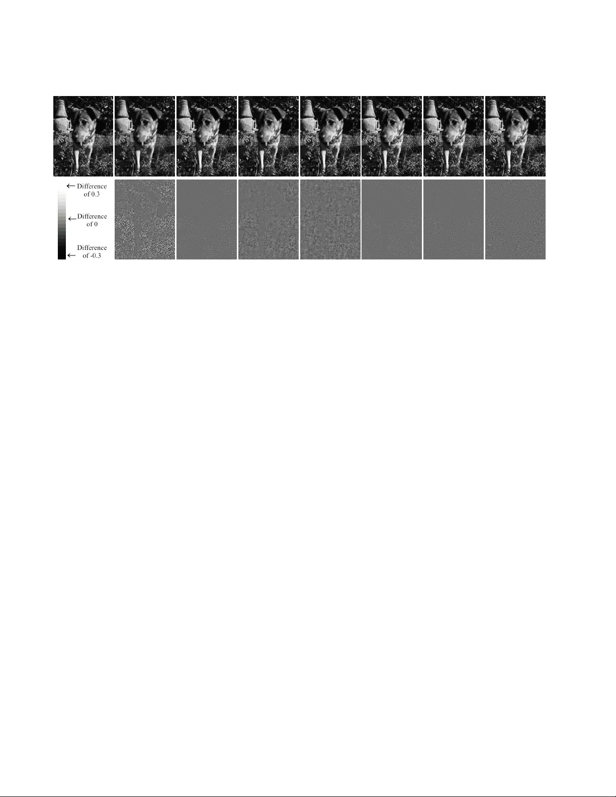
Rob ust Compr essed Sensing and Sparse Coding with the Difference Map W ill Landeck er ∗ Portland State Uni versity landeckw@cs.pdx.edu Rick Chartrand † Los Alamos National Laboratory rickc@lanl.gov Simon DeDeo ∗ Santa Fe Institute Indiana Uni versity simon@santafe.edu Abstract In compr essed sensing, we wish to r econstruct a sparse signal x fr om observed data y . In sparse coding, on the other hand, we wish to find a r epr esentation of an observed signal y as a sparse linear combination, with coefficients x , of elements fr om an over complete dictionary . While many algorithms ar e competitive at both pr oblems when x is very sparse, it can be challenging to r ecover x when it is less spar se. W e pr esent the Difference Map , which excels at sparse reco very when sparseness is lower and noise is higher . The Differ ence Map out-performs the state of the art with r econstruction from r andom measurements and natural image r econstruction via sparse coding. 1. Introduction In compressed sensing (CS), we are giv en a measure- ment matrix Φ ∈ R m × n (where m < n ), observed data y ∈ R m , and we wish to recov er a sparse x ∈ R n such that y = Φ x. The compressed sensing problem can then be written as arg min x k x k 0 subject to y = Φ x, (1) where k · k 0 is the ` 0 penalty function, gi ving the number of nonzero elements. In the noisy case, where ˜ y = Φ x +  · N (0 , σ ) is assumed to be a noisy observation, we often replace the linear constraints with quadratic ones: arg min x k x k 0 subject to k ˜ y − Φ x k 2 2 ≤ δ (2) ∗ This work w as supported by National Science Foundation Grant EF- 1137929, “The Small Number Limit of Biological Information Process- ing, ” and the Emergent Institutions Project. † This work was supported by the U.S. Department of Energy through the LANL/LDRD Program, and by the University of California Laboratory Fees Research Program. for some δ > 0 . The problem (2) can also be used for sparse coding (SC); in this setting, Φ is an overcomplete dictionary , y is a signal (such as an image patch), and we seek a sparse coefficient v ector x . Recently , a v ariety of algorithms have achiev ed good results for a variety of CS and SC problems, including Least Angle Regression (LARS) [12], Subspace Pursuit [9], Matching Pursuit and its variants [11, 19], Iterativ e Hard Thresholding (IHT) and its variants [2 – 4], Iterativ ely Reweighted Least Squares (IRLS) [8], and the Alternating Direction Method of Multipliers (ADMM) [5, 7]. Because solving problems (1) and (2) directly is known to be NP-hard [15], some approaches relax the ` 0 penalty to the con vex ` 1 norm [12, 18], while some attempt to address the ` 0 case directly [4, 9, 19], and still others consider any number of ` p (quasi-)norms for 0 < p ≤ 1 [5, 7, 8]. In gen- eral, the challenge for CS and SC algorithms is to balance two competing constraints on the solution x ∗ : to accurately reconstruct the observed data y , and to be sparse. This paper presents a method for solving CS and SC problems without relaxing the ` 0 constraint, using a gen- eral method known as the Dif ference Map [13]. The Dif- ference Map (DM) has been used to solve a wide variety constraint-intersection problems. Given sets A and B and distance-minimizing projections P A and P B 1 , respectively , DM searches for a point x ∗ ∈ A ∩ B . One iteration of DM is defined by x ← D ( x ) , where D ( x ) = x + β [ P A ◦ f B ( x ) − P B ◦ f A ( x )] (3) where f A ( x ) = P A ( x ) − ( P A ( x ) − x ) /β f B ( x ) = P B ( x ) + ( P B ( x ) − x ) /β and β 6 = 0 . One can test for conv ergence by monitoring the v alue | P A ◦ f B ( x ) − P B ◦ f A ( x ) | , which v anishes when a solution is found. Recently , DM has achieved state-of- the-art performance on a v ariety of NP-hard nonconv ex op- 1 By distance-minimizing projection, we mean that P A ( x 0 ) = min x k x 0 − x k 2 subject to x ∈ A , and like wise for P B . 1 timization problems including protein folding, k -SA T , and packing problems [13]. The rest of this paper is organized as follows. In Sec- tion 2, we introduce an adaptation of the Difference Map for compressed sensing and sparse coding, which we compare at a high le vel to other well-known algorithms. In Section 3, we compare the algorithms on CS problems using random measurements, and we reconstruct natural images via SC in Section 4. 2. Compressed Sensing and Sparse Coding with the Difference Map Giv en a matrix Φ ∈ R m × n (where m < n ) and data y ∈ R m , we wish to find a sparse vector x ∗ ∈ R n that is a solution to problem (2). W e apply the Difference Map to this problem by defining the constraint sets A = { x ∈ R n : k x k 0 ≤ s } B = { x ∈ R n : k Φ x − y k 2 2 < δ } for a pre-defined positiv e integer s and scalar δ > 0 . The minimum-distance projection onto A is known as har d thresholding , and is defined by P A ( x ) = [ x ] s , (4) where [ x ] s is obtained by setting to zero the n − s compo- nents of x ha ving the smallest absolute values. A minimum-distance projection onto the set B inv olves solving a quadratically-constrained quadratic programming problem, which can be very costly . W e approximate this projection with: P B ( x ) = x − Φ + (Φ x − y ) (5) where Φ + = Φ T (ΦΦ T ) − 1 is the Moore-Penrose pseudo- in verse of Φ . The motiv ation for (5) comes from a simplification of our definition for B . Consider the set with linear constraints (as in (1)): { x ∈ R n : Φ x = y } . The minimum distance projection onto this set is given by the linearly constrained quadratic programming (QP) prob- lem P ( x 0 ) = arg min x ∈ R n 1 2 k x − x 0 k 2 2 such that Φ x = y . The Lagrangian of this QP is L ( x, λ ) = 1 2 k x − x 0 k 2 2 + λ (Φ x − y ) . The x that solves the QP is a minimizer of L , and is found by setting ∇ x ( L ) = 0 , which yields x = x 0 + Φ T λ. (6) Plugging (6) into y = Φ x and solving for λ gi ves λ = (ΦΦ T ) − 1 (Φ x 0 − y ) . Finally , we plug this into (6) to get x = x 0 − Φ T (ΦΦ T ) − 1 (Φ x 0 − y ) as in (5). Although the motiv ation for (5) comes from the assump- tion of non-noisy observations y = Φ x , we will see that it performs very well in the noisy case. It is worth noting that the pseudo-in verse is e xpensiv e to compute, though it only needs to be computed once. Thus in the case of sparse image reconstruction where each image patch is reconstructed independently , amortizing the cost of computing Φ + ov er all image patches significantly reduces the pre-computation ov erhead. 2.1. Comparison to Other Algorithms In what follows, we compare the Difference Map to a representativ e sample of commonly-used algorithms for solving CS and SC problems: Least Angle Regres- sion (LARS) [12], Stagewise Orthogonal Matching Pur- suit (StOMP) [11], Accelerated Iterati ve Hard Thresholding (AIHT) [2], Subspace Pursuit [9], Iteratively-Re weighted Least Squares (IRLS) [8] and Alternating Direction Method of Multipliers (ADMM) [5, 7]. As a final point of com- parison, we test the Alternating Map (AM) defined by x ← P A ( P B ( x )) , with P A and P B defined as in (4) and (5), respectiv ely , which resembles the ECME algorithm for known sparsity le vels [16]. The projection P A (4), known as hard thresholding, is an important part of many CS algorithms [2 – 4, 9, 16, 17]. The projection P B (5) also appears in the ECME algorithm [16, 17]. Normalized Iterati ve Hard Thresholding (NIHT) [3] uses a calculation similar to P B , replacing the pseudo- in verse with µ t Φ T for an appropriately chosen scalar µ t . Giv en that many algorithms consider the same types of projections as DM, any advantage achiev ed by DM must not come from the indi vidual projections P A and P B , but rather the way in which DM combines the two projections into a single iterative procedure. This is particularly true when comparing DM to the simple alternating map. Alter- nating between projections is guaranteed to find a point at the intersection of the two constraints if both are conv ex; howe ver , if either of the constraints is not conv ex, it is easy for this scheme to get stuck in a local minimum that does not belong to intersection. While many of the theoretical questions about the Dif- ference Map remain open, it does come with a crucial guar- antee here: e ven on noncon vex problems, a fixed point (meaning D ( x ) = x ) implies that we have found a solution 2 (meaning a point in A ∩ B ). T o see this, note that D ( x ) = x implies P A ◦ f B ( x ) = P B ◦ f A ( x ) . (7) Thus we have found a point that exists in both A and B . This leads us to believ e that DM will find better sparse so- lutions when other algorithms are stuck in local minima. Note that we are not the first to consider applying DM to compressed sensing. Qiu and Dogand ˇ zi ´ c [17] apply DM to the ECME algorithm (a v ariant of expectation maximiza- tion) in order to improve upon one of the two projections inside that algorithm. Although one of ECME’ s two pro- jections uses DM internally , ECME continues to combine the two projections in a simple alternating fashion. This is in stark contrast to our proposed algorithm, which uses DM externally to the individual projections as a more intricate way of combining them. The resulting algorithm, called DM-ECME, is intended only for compressed sensing with non-negati ve signals. Because we consider different types of problems in this paper , we do not include DM-ECME in the comparisons below . 2.2. Implementation Details W e implemented the Dif ference Map in Matlab (code is av ailable online 2 ). All experiments were performed on a computer with a 3 GHz quad-core Intel Xeon processor , running Matlab R2011a. W e obtained Matlab implemen- tations of LARS and StOMP from SparseLab v2.1 [1]. Im- plementations of AIHT [2] and Subspace Pursuit [9] were found on the websites of the papers’ authors. W e also ob- tained Matlab implementations of ADMM [7] and IRLS [8] directly from the authors of the cited papers. The implementations of LARS, Subspace Pursuit, AIHT , and StOMP are parameter-free. It was necessary to tune a single parameter for DM, and two parameters each for ADMM and IRLS. W e tuned the parameters in two itera- tions of grid search. ADMM and IRLS required different parameters for the two different experiments presented in this paper (reconstruction from random measurements, and natural image reconstruction). Interestingly , DM performed well with the same parameter for both types of e xperiments. W e use “training” matrices of the same dimension, spar - sity , and noise level as the ones presented in the figures of this paper in order to tune parameters. W e chose parameters to minimize the MSE of the recov ering x , av eraged ov er all training problems. When tuning parameters for natural im- age reconstruction, we used a training set of 1000 image patches taken from the person and hill categories of Ima- geNet [10], providing a good v ariety of natural scenery . When tuning β for DM, we first perform grid search with an interv al of 0 . 1 , between − 1 . 2 and 1 . 2 3 . Next, in a radius 2 http://web.cecs.pdx.edu/ ˜ landeckw/dm- cs0 3 The natural range for the parameter β is [-1,1] (excluding 0), but of 0 . 5 around the best β , we performed another grid search with an interval of 0 . 01 . Surprisingly , all β in the interval [ − 0 . 9 , − 0 . 1] appeared to be equally good for all problems reported in this paper . W e chose β = − 0 . 14 because it performed slightly better during our experiments, but the advantage o ver other β ∈ [ − 0 . 9 , − 0 . 1] was not significant. W e use logarithmic grid search to tune the two pa- rameters for ADMM and IRLS. First, we search param- eter values by powers of ten, meaning 10 α , for α = − 5 , − 4 , . . . , 5 . W e then search in the neighborhood of best exponent c by 1 10 powers of ten, meaning 10 c + α for α = − 0 . 5 , − 0 . 4 , . . . , 0 . 5 . For random measurements (the experiments in Sec- tion 3), this results in parameter v alues µ = 1 . 26 × 10 2 , λ = 3 . 98 × 10 − 1 for ADMM, and α = 3 . 16 × 10 − 3 ; β = 2 . 51 × 10 − 1 . For natural image reconstruction (Section 4), we found µ = 1 . 58 × 10 2 , λ = 1 . 0 × 10 − 1 for ADMM and α = 2 . 5 × 10 − 4 , β = 5 × 10 − 3 for IRLS. Note that the β pa- rameter for IRLS has nothing to do with the β parameter for DM. W e refer to both as β only to remain consistent with the respecti ve bodies of literature about each algorithm, b ut in what follows we will only refer to the parameter for DM. IRLS is capable of addressing the ` p quasi-norm for a vari- ety of v alues 0 < p ≤ 1 , while ADMM uses modifications of the ` p quasi-norm designed to hav e a simple proximal mapping [6]. In both cases we tried p = 1 2 and p = 1 , and found p = 1 2 to perform better . 3. Random Measurements In this Section, we compare the performance of DM to other algorithms when reconstructing signals from random measurements, testing a wide v ariety of matrix sizes, spar- sity , and noise levels. Gi ven positi ve integers m, n, and s , we generate the random matrix Φ ∈ R m × n with entries drawn from N (0 , 1) . W e then ensure that columns hav e zero mean and unit norm. W e generate the s -sparse vector x ∈ R n whose nonzero elements are drawn from N (0 , 1) . W e then calculate y = Φ x , and the noisy “observation” ˜ y = y +  · N (0 , 1) . Finally , we ask each algorithm to reconstruct x gi ven only Φ and ˜ y . W e measure runtime instead of iterations, as the time re- quired per iteration v aries widely for the algorithms con- sidered. Additionally , the pre-computation for DM is the longest of any algorithm, requiring the pseudo-in verse of the dictionary . This pre-computation overhead is included in the timekeeping. In the first e xperiment, each algorithm attempts to recon- struct x as we v ary the sparsity lev el s . W e choose  so that the signal-to-noise ratio (SNR) is close to 20 dB. The re- sults in Figure 1 demonstrate that for small values of s (left, Elser et al . [13] report that occasionally v alues outside of this interval work well. 3 0.1 0.2 0.3 0.4 0.5 0.6 0.7 0 10 20 30 40 50 t ( s e c on d s ) | | x − x t | | 2 m = 4 0 0 , n = 1 0 0 0 , s = 5 0 , S N R = 1 9 . 2 2 d B DM A D M M I R L S L A R S S u b s pa c e P u r s u i t S t O M P A I H T A M 0.05 0.1 0.15 0.2 0.25 0.3 0.35 0.4 0 20 40 60 80 100 120 t ( s e c on d s ) | | x − x t | | 2 m = 4 0 0 , n = 1 0 0 0 , s = 1 0 0 , S N R = 2 0 . 1 3 d B DM A D M M I R L S L A R S S u b s pa c e P u r s u i t S t O M P A I H T A M 0.05 0.1 0.15 0.2 0.25 0.3 0.35 0.4 0 20 40 60 80 100 120 140 t ( s e c on d s ) | | x − x t | | 2 m = 4 0 0 , n = 1 0 0 0 , s = 1 5 0 , S N R = 2 0 . 9 8 d B DM A D M M I R L S L A R S S u b s pa c e P u r s u i t S t O M P A I H T A M Figure 1. Reconstructing signals with various lev els of sparsity s . W ith sparser signals (left, middle), most algorithms get very close to the true signal. W ith less sparse signals (right), the Dif ference Map gets closer than other algorithms to recov ering the signal. Each plot is av eraged ov er ten runs, with  chosen to giv e an SNR of approximately 20 dB, and Φ ∈ R 400 × 1000 . 0.05 0.1 0.15 0.2 0.25 0.3 0.35 0.4 0 20 40 60 80 100 120 140 160 t ( s e c on d s ) | | x − x t | | 2 m = 4 0 0 , n = 1 0 0 0 , s = 1 5 0 , S N R = 2 3 . 0 3 d B DM A D M M I R L S L A R S S u b s pa c e P u r s u i t S t O M P A I H T A M 0.05 0.1 0.15 0.2 0.25 0.3 0.35 0.4 0 20 40 60 80 100 120 140 t ( s e c on d s ) | | x − x t | | 2 m = 4 0 0 , n = 1 0 0 0 , s = 1 5 0 , S N R = 1 8 . 5 5 d B DM A D M M I R L S L A R S S u b s pa c e P u r s u i t S t O M P A I H T A M 0.05 0.1 0.15 0.2 0.25 0.3 0.35 0.4 0 20 40 60 80 100 120 140 t ( s e c on d s ) | | x − x t | | 2 m = 4 0 0 , n = 1 0 0 0 , s = 1 5 0 , S N R = 1 7 . 5 5 d B DM A D M M I R L S L A R S S u b s pa c e P u r s u i t S t O M P A I H T A M Figure 2. Reconstructing signals with various levels of noise  . W ith less noise (left), most algorithms get very close to the true signal. W ith more noise (middle, right), the Difference Map gets closer than other algorithms to recov ering the signal. Each plot is a veraged over ten runs, with s = 150 and Φ ∈ R 400 × 1000 . middle), meaning sparser signals, most algorithms are able to recov er x almost perfectly . As we increase the v alue of s (right), meaning denser signals, other algorithms con ver ge to undesirable minima. The Dif ference Map, howe ver , con- tinues to get very close to reco vering x . In the next experiment, each algorithm attempts to re- construct x as we vary the noise by changing  . s is fixed at 150. The results in Figure 2 show that with less noise (left), meaning lower  and higher SNR, sev eral algorithms are able to get close to recovering the true signal x . As the noise increases (middle, right), meaning higher  and lo wer SNR, only the Dif ference Map is able to get close to reco v- ering the signal. Note that DM and AM start “late” in all plots from Figures 1 and 2 because their pre-computation time is the longest (calculating Φ + ). Despite using the same projec- tions, we notice a large disparity in performance between DM and AM when s = 150 . Because the two algorithms both use the same two projections P A and P B , this per- formance gap shows the power of combining two simple projections in a more elaborate way than simply alternating between them. From the results in Figures 1 and 2, we hypothesize that DM has a significant advantage with noisy , less sparse signals (higher  and s ) where other state-of-the-art com- pressed sensing algorithms get stuck in local minima or re- quire a large amount of time to reach a good solution. W e test this hypothesis with a variety of different matrix sizes in Figure 3, each time with a sparsity ratio s/n of approxi- mately 1 / 3 and an SNR of approximately 20 dB. The results show that DM does indeed outperform other algorithms in this setting, for all matrix sizes tested. 4. Sparse Coding Image Reconstruction The results from Section 3 indicate that DM offers an ad- vantage over other algorithms when the underlying signal is less sparse and the observation is noisy . The less-sparse, noisy setting corresponds well to images which contain a large variety of te xtures, such as natural images. In this Sec- tion, we measure the sparse coding performance of the same algorithms as in the previous section (with the exception of AM, whose sparse coding performance was not competi- tiv e), by comparing reconstruction quality for a variety of images. When reconstructing a lar ge image, we treat each w × w patch as an independent signal to reconstruct. Because our 4 0.5 1 1.5 2 2.5 3 3.5 4 0 50 100 150 200 250 300 350 400 450 t ( s e c o n d s ) | | x − x t | | 2 m = 1 02 4 , n = 2 0 4 8 , s = 4 0 0 , S N R = 1 9 . 6 9 d B DM A D M M I R L S L A R S S u b s p a c e P ur s u i t S t OM P A I H T A M 5 10 15 20 0 100 200 300 400 500 600 700 800 900 t ( s e c o n d s ) | | x − x t | | 2 m = 2 00 0 , n = 5 0 0 0 , s = 8 0 0 , S N R = 2 0 . 0 8 d B DM A D M M I R L S L A R S S u b s p a c e P ur s u i t S t OM P A I H T A M 10 20 30 40 50 60 0 200 400 600 800 1000 1200 t ( s e c o n d s ) | | x − x t | | 2 m = 3 00 0 , n = 8 0 0 0 , s = 1 0 5 0 , S N R = 1 9 . 8 6 d B DM A D M M I R L S L A R S S u b s p a c e P ur s u i t S t OM P A I H T A M Figure 3. In the lo w sparsity regime, the difference map outperforms other algorithms at recovering x from a noisy observed signal with a wide variety of matrix sizes. The sparsity ratio s/n is approximately 1/3, and the noisy observation ˜ y = Φ x +  · N (0 , 1) has an SNR of approximately 20 dB. Each plot is av eraged ov er ten runs. dictionary is constant, we only need to compute the pseudo- in verse in (5) once. By amortizing the cost of the pseudo- in version over all patches, this effecti vely allows DM to con verge in less time per patch. W e amortize the cost of pre-computation for other algorithms as well (most notably ADMM and IRLS). In order to test the performance of the algorithms when reconstructing natural images, we require a dictionary learned for sparse image reconstruction. Dictionary learn- ing is not the focus of this paper , but we present our method for completeness. The dictionary is trained with 10 mil- lion 20 × 20 image patches, and we choose to learn 1000 atoms, resulting in a dictionary of size 400 × 1000 . W e train the dictionary with patches from the person and hills category of ImageNet [10], which provide a variety of nat- ural scenery . W e alternate sparse coding using 20 iterations of ADMM using p -shrinkage with p = 1 / 2 (see [6] for de- tails), with a dictionary update using the method of optimal directions [14]. W e used ADMM as the sparse-coding al- gorithm simply because we had access to MPI-parallelized C code for this purpose. W e do not belie ve that this gav e an unfair adv antage to ADMM, because the reconstructed images presented in this paper are separate from the dataset used to train the dictionary . Using 1,000 processors, the dictionary conv erged in about 2.5 hours. The training patches were reconstructed by the dictionary with an av erage of 29 nonzero components (out of 1000), and the reconstruction of the training images had a relativ e error of 5.7%. The dictionary contains the typical combination of high- and low-frequenc y edges, at various orientations and scales. Some examples are shown in Figure 4. W e reconstruct se veral natural images and measure the quality of the sparse reconstruction as a function of time. At time t , we measure the reconstruction quality of patch y as follows. First, we perform hard-thresholding on the algo- rithm’ s current guess x t , setting the n − s smallest absolute values to zero, yielding the s -sparse vector [ x t ] s . W e then Figure 4. Example atoms from the dictionary Φ ∈ R 400 × 1000 used for reconstruction. The dictionary contains elements of size 20 × 20 , learned from 10 million image patches from the person and hill categories of ImageNet [10]. calculate the reconstruction y t = Φ[ x t ] s and measure the SNR of y (the true image patch) to y t . Thus we are measuring how well, at time t , the algorithm can create a sparse reconstruction of y . Note that algorithms returning a solution that is sparser than required will not be affected by the hard-thresholding step. W e reconstruct a 320 × 240 image of a dog, seen in Fig- ure 5, using the 400 × 1000 dictionary from Figure 4. W e measure results for both s = 100 and s = 200 , as well as t = 0 . 05 and t = 0 . 1 4 . The results in T able 1 show that DM consistently achieves the highest SNR. Furthermore, while increasing s and t tend to improve each algorithm’ s reconstruction, the relative quality between algorithms stays fairly consistent. 4 W e measure time in seconds per 20 × 20 patch. Thus t = 0 . 05 cor- responds to approximately 10 seconds for the entire image, and t = 1 to 20 seconds for the entire images. The astute reader will notice that when Φ has dimension 400 × 1000 , it takes longer than 0.1 seconds to com- pute Φ + . This can be seen in Figures 1 and 2, where it takes almost 0.2 seconds for DM to finish calculating Φ + and begin searching for x . How- ev er , because we only need to calculate the pseudo-inv erse once for the entire image, this start-up cost is amortized over all patches and becomes negligible. 5 T able 1. Signal to noise ratio (SNR, in decibels) of the recon- structed image from Figure 5. W e test various sparsity levels s and various runtimes (seconds per 20 × 20 patch). The dif ference map consistently achiev es the highest SNR. s = 100 s = 100 s = 200 s = 200 t = 0 . 05 t = 0 . 1 t = 0 . 05 t = 0 . 1 Diff. Map 17.02 17.55 22.44 23.73 ADMM 15.27 16.59 19.37 21.71 IRLS 13.39 14.87 18.14 20.57 Sub . Pursuit 16.58 16.67 16.99 16.97 LARS 11.35 13.88 11.30 13.93 AIHT 14.78 15.70 18.79 19.94 StOMP 15.40 15.39 17.84 17.91 The highest quality reconstructions, achiev ed with s = 200 and t = 0 . 1 , are shown in Figure 5 (top row). While some algorithms fail to reconstruct details in the animal’ s fur and the grass, many algorithms reconstruct the image well enough to make it dif ficult to find errors by mere visual inspection. W e sho w the difference between the reconstruc- tions and the original image (Figure 5, bottom row), where a neutral gray color in the difference image corresponds to a perfect reconstruction of that pixel; white and black are scaled to a difference of 0.3 and -0.3, respecti vely (the orig- inal image was scaled to the interv al [0,1]). The advantage of DM over other algorithms, when sparsely reconstructing images, can be seen with a large v a- riety of images. In Figure 6, we see that DM consistently achiev es the best reconstruction. All original images are av ailable online 5 . 5. Conclusions W e have presented the Difference Map, a method of find- ing a point at the intersection of two constraint sets, and we hav e introduced an implementation of DM for compressed sensing and sparse coding. The constraint-set formulation is a natural fit for sparse recovery problems, in which we hav e two competing constraints for x : to be consistent with the data y , and to be sparse. When the solution x is very sparse and the observation ˜ y is not too noisy , DM takes more time in finding the same solution as competing algorithms. Howe ver , when the so- lution x is less sparse and when the observation ˜ y is noisy , DM outperforms state of the art sparse reco very algorithms. The noisy , less sparse setting corresponds well to recon- structing natural images, which can often require a large number of components in order to accurately reconstruct. Experiments show that DM performs fav orably in recon- structing a variety of images, with a variety of parameter 5 http://web.cecs.pdx.edu/ ˜ landeckw/dm- cs0 Difference Map 23.33 ADMM 20.80 IRLS 20.50 LARS 13.62 Subspace Pursuit 17.96 StOMP 19.48 AIHT 19.41 Difference Map 23.06 ADMM 20.67 IRLS 20.59 LARS 14.37 Subspace Pursuit 17.44 StOMP 18.78 AIHT 19.44 Difference Map 25.39 ADMM 22.72 IRLS 23.55 LARS 17.60 Subspace Pursuit 20.66 StOMP 23.37 AIHT 21.98 Difference Map 23.95 ADMM 21.90 IRLS 20.90 LARS 14.27 Subspace Pursuit 17.14 StOMP 17.97 AIHT 20.34 Figure 6. The Difference Map regularly outperforms other algo- rithms in finding sparse reconstructions of a v ariety of images. W e measure the SNR in decibels (right column) between the recon- struction and the original image (left column). Images are scaled to 240 × 320 pixels ( 320 × 240 for horizontal images). Recon- structions ha ve sparsity s = 200 , and are completed in 20 seconds per image (approximately 0.1 seconds per 20 × 20 patch). The dictionary Φ is the same as in Figure 4. settings. Parameter tuning can present a laborious hurdle to the re- searcher . DM requires tuning only a single parameter β . For all experiments in this paper (natural image reconstruction for various images; reconstruction with random matrix dic- tionaries of v arious sizes, with varying amounts of sparsity and noise), we found DM to w ork almost equally as well for all − 0 . 9 ≤ β ≤ − 0 . 1 . The robustness of DM under such a wide v ariety of parameter v alues and problems makes DM a very competiti ve choice for compressed sensing. The robustness of DM comes from how it combines two simple projections into a single iterativ e procedure. The Alternating Map (AM) combines the same projections in a simple alternating fashion, and struggles in almost all exper- iments. The gap in performance between these tw o methods 6 Original LARS StOMP IRLS ADMM Sub. Pursuit AIHT Diff. Map 13.93 dB 17.91 dB 20.57 dB 21.71 dB 16.97 dB 19.94 dB 23.73 dB Figure 5. Reconstructing a natural image. The Difference Map outperforms the other algorithms when reconstructing a 320 × 240 image of a dog (top). Difference images (bottom) show the dif ference between the reconstruction and the original image, which ranges from -0.3 (black) to 0.3 (white) – original grayscale values are between 0 (black) and 1 (white). Results for s = 200 are sho wn, and the time limit was 0.1 seconds per 20 × 20 patch. demonstrates the power of combining multiple constraints in a more perspicacious way . Finally , we recall that performance in all experiments was measured as a function of time, which would seem to put DM at a natural disadvantage to other algorithms: DM requires the pseudo-in verse of the dictionary , computing which requires more time than any other algorithm’ s pre- computation. Despite this, DM consistently outperforms other algorithms. References [1] SparseLab Matlab Softw are. http://sparselab. stanford.edu . [2] T . Blumensath. Accelerated iterati ve hard thresholding. Sig- nal Pr ocessing , 92(3):752 – 756, 2012. [3] T . Blumensath and M. E. Davies. Iterati ve hard thresholding for compressed sensing. Applied and Computational Har- monic Analysis , 27(3):265–274, 2009. [4] T . Blumensath and M. E. Da vies. Normalized iterati ve hard thresholding: Guaranteed stability and performance. IEEE Journal of Selected T opics in Signal Pr ocessing , pages 298– 309, 2010. [5] S. Boyd, N. Parikh, E. Chu, B. Peleato, and J. Eckstein. Dis- tributed optimization and statistical learning via the alternat- ing direction method of multipliers. F oundations and T r ends in Machine Learning , 3(1):1–122, 2011. [6] R. Chartrand. Noncon vex splitting for regularized low-rank + sparse decomposition. IEEE T ransactions on Signal Pro- cessing , 60:5810–5819, 2012. [7] R. Chartrand and B. W ohlberg. A noncon vex ADMM algo- rithm for group sparsity with sparse groups. In IEEE Inter- national Conference on Acoustics, Speech, and Signal Pro- cessing , 2013. [8] R. Chartrand and W . Y in. Iterativ ely re weighted algorithms for compressi ve sensing. In IEEE International Confer ence on Acoustics, Speech and Signal Pr ocessing , pages 3869– 3872, 2008. [9] W . Dai and O. Milenkovic. Subspace pursuit for compressive sensing signal reconstruction. IEEE T ransactions on Infor- mation Theory , 55(5):2230–2249, 2009. [10] J. Deng, W . Dong, R. Socher , L.-J. Li, K. Li, and L. Fei-Fei. ImageNet: A Large-Scale Hierarchical Image Database. In IEEE Conference on Computer V ision and P attern Recogni- tion , 2009. [11] D. L. Donoho, Y . Tsaig, I. Drori, and J.-L. Starck. Sparse solution of underdetermined systems of linear equations by stagewise orthogonal matching pursuit. IEEE T ransactions on Information Theory , 58(2):1094–1121, 2012. [12] B. Efron, T . Hastie, I. Johnstone, and R. T ibshirani. Least angle regression. Annals of Statistics , 32:407–499, 2004. [13] V . Elser , I. Rankenbur g, and P . Thibault. Searching with it- erated maps. Proceedings of the National Academy of Sci- ences , 104(2):418–423, 2007. [14] K. Engan, S. Aase, and J. Hakon Husoy . Method of opti- mal directions for frame design. In IEEE International Con- fer ence on Acoustics, Speech, and Signal Processing , pages 2443–2446, 1999. [15] B. K. Natarajan. Sparse approximate solutions to linear sys- tems. SIAM Journal on Computing , 24(2):227–234, 1995. [16] K. Qiu and A. Dogand ˇ zi ´ c. Double overrelaxation threshold- ing methods for sparse signal reconstruction. In Information Sciences and Systems , pages 1–6. IEEE, 2010. [17] K. Qiu and A. Dogand ˇ zi ´ c. Nonnegati ve signal reconstruction from compressiv e samples via a dif ference map ECME algo- 7 rithm. In IEEE W orkshop on Statistical Signal Pr ocessing , pages 561–564, 2011. [18] R. T ibshirani. Regression shrinkage and selection via the lasso. Journal of the Royal Statistical Society . Series B (Methodological) , pages 267–288, 1996. [19] J. A. Tropp and A. C. Gilbert. Signal recovery from random measurements via orthogonal matching pursuit. IEEE T rans- actions on Information Theory , 53(12):4655–4666, 2007. 8