Estimating Functions of Distributions Defined over Spaces of Unknown Size

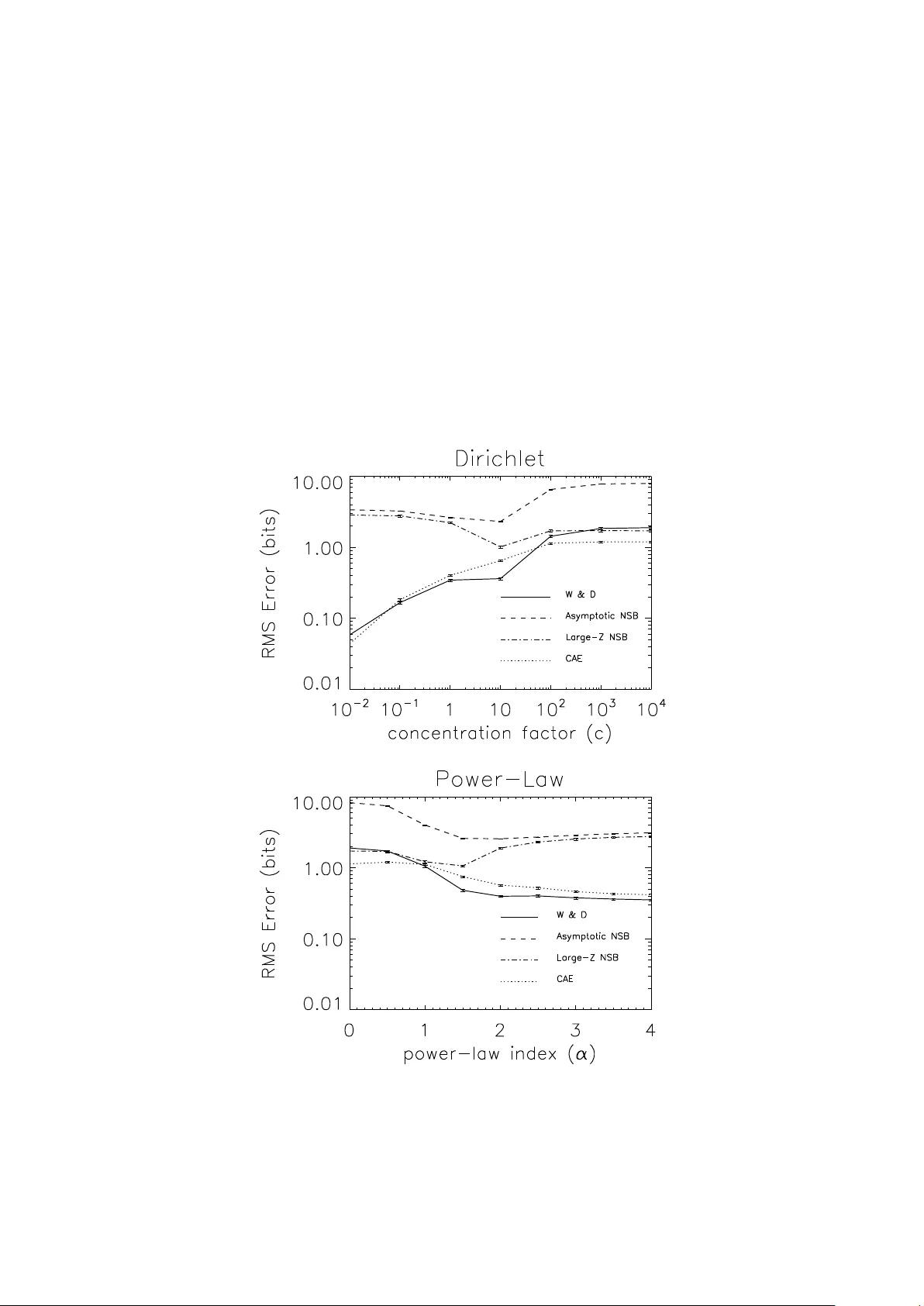
Entr opy 2013 , 15 , 4668-4699; doi:10.3390/e15114668 OPEN A CCESS entropy ISSN 1099-4300 www .mdpi.com/journal/entrop y Article Estimating Functions of Distrib utions Deﬁned over Spaces of Unknown Size Da vid H. W olpert 1 , * and Simon DeDeo 1 , 2 1 Santa Fe Institute, 1399 Hyde Park Rd., Santa Fe, NM 87501, USA; E-Mail: simon@santafe.edu 2 School of Informatics and Computing, Indiana Uni versity , 901 E 10th St, Bloomington, IN 47408, USA * Author to whom correspondence should be addressed; E-Mail: david.h.wolpert@gmail.com. Received: 3 August 2013; in r evised form: 11 September 2013 / Accepted: 17 October 2013 / Published: 31 October 2013 Abstract: W e consider Bayesian estimation of information-theoretic quantities from data, using a Dirichlet prior . Ackno wledging the uncertainty of the e vent space size m and the Dirichlet prior’ s concentration parameter c , we treat both as random v ariables set by a hyperprior . W e sho w that the associated hyperprior , P ( c, m ) , obeys a simple “Irrele vance of Unseen V ariables” (IUV) desideratum iff P ( c, m ) = P ( c ) P ( m ) . Thus, requiring IUV greatly reduces the number of degrees of freedom of the hyperprior . Some information-theoretic quantities can be expressed multiple ways, in terms of different ev ent spaces, e.g., mutual information. W ith all hyperpriors (implicitly) used in earlier work, dif ferent choices of this ev ent space lead to different posterior expected values of these information-theoretic quantities. W e sho w that there is no such dependence on the choice of e vent space for a hyperprior that obeys IUV . W e also deri ve a result that allo ws us to exploit IUV to greatly simplify calculations, lik e the posterior e xpected mutual information or posterior expected multi-information. W e also use computer experiments to fa vorably compare an IUV -based estimator of entropy to three alternati ve methods in common use. W e end by discussing how seemingly innocuous changes to the formalization of an estimation problem can substantially af fect the resultant estimates of posterior expectations. K eywords: Bayesian analysis; entropy; mutual information; variable number of bins; hidden v ariables; Dirichlet prior Entr opy 2013 , 15 4669 1. Background A central problem of statistics is estimating a functional of a probability distribution ρ from a dataset, ~ n , of N independent, identically distributed (IID) samples of ρ . A simple example of this problem is estimating the mean Q ( ρ ) of a distribution, ρ , from a set of IID samples of that distribution. In this example, the functional Q ( . ) depends linearly on ρ . More challenging versions of this problem arise when the functional Q ( . ) is nonlinear . In particular , recent decades ha ve seen a lot of work on estimating information-theoretic functionals [ 1 , 2 ] of a distribution from a set of IID samples of that distribution. Examples include estimating the Shannon entropy of the distribution, its mutual information, etc ., from such a set of samples and, in particular , using the bootstrap to estimate associated error bars [ 3 – 5 ]. This w ork has concentrated on the case where the ev ent space being sampled is countable. In addition, much of it has used non-Bayesian approaches. The ﬁrst work that addressed the problem using Bayesian techniques was the sequence of papers [ 6 – 8 ] (hereafter abbreviated as WW), followed by similar work in [ 9 ] (see Appendix A for a list of corrections to some algebraic mistakes in [ 6 ]; a careful analysis of the numerical implementation of the formulas in WW can be found in [ 10 ]). This work showed ho w to calculate posterior moments of sev eral nonlinear functionals of the distribution. Such moments provide both the Bayes-optimal estimate of the functional (assuming a quadratic loss function) and an error bar in that estimate. In particular , WW provided closed-form expression for the posterior ﬁrst and second moments of entropy , mutual information and Kullback-Leibler distance, in addition to various non-information-theoretic quantities, like co variance. Write the space of possible ev ents as Z with elements written as z and distributions over Z as ρ . For tractability reasons, WW used a Dirichlet prior o ver the associated simple x of possible distrib utions, P ( ρ ) ∝ Q z ρ ( z ) cL ( z ) − 1 . (In the literature, the constant, c , is sometimes called a concentration parameter, and L is sometimes called a baseline distribution.) In WW , Z was taken to be ﬁxed (not a random v ariable), L ( z ) was taken to be uniform ov er Z and c was taken to equal | Z | , the size of Z . This choice of a Dirichlet prior ov er ρ with uniform L has been the basis of all subsequent work on Bayesian estimates of information-theoretic functionals of distributions [ 11 , 12 ]. (Note though that recently , there has been some inv estigation of the extension of this work to mixture-of-Dirichlet distributions [ 12 ] and Dirichlet / Pittman-Y or processes [ 11 ]).) Ho wever , there has not been such consensus concerning c . Although the choice of c = | Z | was not explicitly advocated in WW , all the results in WW are for this special case. An important series of papers [ 12 – 14 ] (hereafter abbreviated as NSB) considered the generalization where c = a | Z | for any positi ve constant, a . (WW is the special case where a = 1 .) NSB considered the limit where we hav e such a c , and | Z | is much lar ger than N , the number of samples of ρ . (Therefore, for non-inﬁnitesimal a , c  N .) They sho wed that in this limit, the samples hav e little ef fect on the posterior moments of Q (e.g., for Q the Shannon entropy). Therefore, the data become irrele vant. In that large | Z | limit, the posterior moments are dominated by the prior ov er ρ that is speciﬁed by c . This can be seen as a major shortcoming of WW . Entr opy 2013 , 15 4670 T o address this shortcoming, NSB noted that if c is a random variable with an associated prior , P ( c ) , it induces a prior distribution ov er the values of the Shannon entropy , H ( ρ ) = − P z ρ ( z ) ln[ ρ ( z )] . Speciﬁcally , for the case of a uniform L , for any potential entropy v alue h : P ( H = h ) = Z dcdρ δ ( H ( ρ ) − h ) P ( ρ | c ) P ( c ) = Z dcdρ δ ( H ( ρ ) − h ) Q z ρ ( z ) c/ | Z |− 1 R dρ 0 Q z ρ 0 ( z ) c/ | Z |− 1 P ( c ) (1) where the integrals ov er distributions are implicitly restricted to the associated simplex. NSB then decided that since their goal was to estimate entropy , they would set P ( c ) so that the prior , P ( H ) , is ﬂat. In essence, they formed a continuous mixture of Dirichlet distributions to (attempt to) obtain a ﬂat prior ov er the ultimate quantity of interest, H . The P ( c ) that results in ﬂat P ( H ) cannot be written do wn in closed form, but NSB sho wed ho w numerical computations can be used to approximate it. As they are used in practice, both NSB and WW allo w | Z | to vary , giving it dif ferent v alues for dif ferent problems, values that are typically set in an ad hoc way . (Indeed, if they did not allow the number of bins to vary from one dataset to another , they could not be used on problems with datasets running ov er too large a number of bins.) They then set P ( c ) based on that ﬁxed v alue of | Z | . One problem with this is that it means the posterior expected value of the functional, Q , can v ary depending on how one expresses that functional. T o illustrate this, say that Z is a Cartesian product, X × Y , and let H ( X , Y ) , H ( X ) and H ( Y ) refer to the entropies of ρ ( x, y ) ≡ ρ X,Y ( x, y ) , ρ ( x ) ≡ ρ X ( x ) ≡ P y ρ ( x, y ) and ρ ( y ) ≡ ρ Y ( y ) ≡ P x ρ ( x, y ) , respectiv ely . Recall that the mutual information between X and Y under any ρ can be written both as: I ρ ( X ; Y ) ≡ − X x ρ ( x ) ln[ ρ ( x )] − X y ρ ( y ) ln[ ρ ( y )] + X x,y ρ ( x, y ) ln[ ρ ( x, y )] = H ( X ) + H ( Y ) − H ( X , Y ) (2) and equi valently as: I ρ ( X ; Y ) ≡ X x,y ρ ( x, y ) ln  ρ ( x, y ) ρ ( x ) ρ ( y )  (3) No w , let ~ n be a set of IID of samples of ρ X,Y , and let ~ n X and ~ n Y be the associated set of sample v alues of ρ X and ρ Y , respectiv ely . Then, from Equations ( 2 ) and ( 3 ), the posterior expectation of the mutual information can be written as either: E ( I ( X ; Y ) | ~ n ) = − E  X x ρ X ( x ) ln[ ρ X ( x )] | ~ n X  − E  X y ρ Y ( y ) ln[ ρ Y ( y )] | ~ n Y  + E  X x,y ρ ( x, y ) ln[ ρ ( x, y )] | ~ n  = E ( H ( X ) | ~ n X ) + E ( H ( Y ) | ~ n Y ) − E ( H ( X , Y ) | ~ n ) (4) or as: E ( I ( X ; Y ) | ~ n ) = E  X x,y ρ ( x, y ) ln  ρ ( x, y ) ρ ( x ) ρ ( y )      ~ n  (5) Entr opy 2013 , 15 4671 (See, for example, [ 11 , 15 ].) If P ( c ) is set in a way that depends on the size of the event space, then we would use a different P ( c ) to ev aluate each of the three terms in Equation ( 4 ), since the underlying ev ent spaces ( X , Y and X × Y , respectiv ely) hav e different sizes. Ho wever , there would only be a single P ( c ) used to ev aluate the expression in Equation ( 5 ), the same P ( c ) as used for ev aluating the third term in Equation ( 4 ). As a result, under either the NSB or WW approaches, the v alues gi ven by Equation ( 4 ) and Equation ( 5 ) will differ in general; depending on which deﬁnition of mutual information we adopt, we would get a dif ferent estimate of posterior expected mutual information under those approaches. Indeed, to estimate mutual information in the NSB approach, one faces the choice of whether to set P ( c ) to giv e a uniform prior distrib ution ov er values of the mutual information, P ( I ( X ; Y )) (as it would appear , one must, since I ( X ; Y ) is what one wishes to estimate), or to set it to giv e a uniform P ( H ( X , Y )) (as in con ventional NSB). It is not clear ho w to make this choice, in general. 2. Contribution of This P aper In most of the earlier work on estimating an information-theoretic functional of ρ based on data, it is assumed that | Z | is ﬁxed, with a few exceptions (see, e.g., [ 16 ]). In many situations, the modeler is not completely certain a priori about the value of | Z | , and so should treat it as a random v ariable. For such scenarios, we need to specify a joint (hyper)prior , P ( c, | Z | ) , rather than just a prior, P ( c ) . In particular , if we set c from | Z | as in either WW or NSB, then by specifying our uncertainty in Z , P ( | Z | ) , we set the joint prior P ( c, | Z | ) . Note that for both WW and NSB, this induced P ( c, | Z | ) is not a product distribution P ( c ) P ( | Z | ) . (In particular , in NSB, the distribution, P ( c ) , is set independently of any data, in a way that v aries with | Z | .) Jaynes has argued con vincingly for setting priors with in variance arguments concerning the fundamental nature of the problem domain [ 17 ]. In this paper , we show that the prior , P ( c, | Z | ) , obeys a simple “Irrele vance of Unseen V ariables” (IUV) in variance, if and only if c and | Z | are independent, i.e. , if f P ( c, | Z | ) = P ( c ) P ( | Z | ) . Therefore, if we require IUV , then rather than specify a full joint distribution ov er c and | Z | , we only need to specify a distrib ution ov er each of c and | Z | separately . This greatly reduces the number of degrees of freedom in the prior that we need to specify (though not as much as would be the case if we used WW or NSB, were we only to specify P ( | Z | ) ). In this paper , we sho w that when IUV is obeyed, so that c and | Z | are independent, the value for posterior expected mutual information does not change depending on whether we use Equation ( 2 ) or Equation ( 3 ) to deﬁne mutual information. In proving this, we deriv e an intermediate result that simpliﬁes the calculation of some posterior moments. In particular, we sho w how to use this result to deri ve the formula for posterior expected mutual information giv en in WW in essentially a single line. W e also show that both of these advantages extend to the calculation of multi-information, one of the ways proposed to generalize mutual information beyond two random v ariables [ 18 ]. Similarly , since Tsallis entropy with index q is just a weighted sum ov er i of the q th moments of the p i , we can ev aluate expected Tsallis entropy in closed form using our estimators. (Howe ver , higher-order moments of the Tsallis entropy do not simplify as easily .) Entr opy 2013 , 15 4672 W e then show that when c and | Z | are independent under the prior , and | Z | is a veraged ov er according to a prior P ( | Z | ) with some reasonable characteristics, the posterior expected v alue of information-theoretic quantities need not be dominated by the prior . In this sense, the problem that caused NSB to consider a non-con ventional scheme for setting P ( c ) does not exist if we allo w | Z | to be a random v ariable and require IUV . W e next discuss in detail v arious fully Bayesian schemes in which the random v ariables, c and/or | Z | , are integrated over to form estimates of posterior expectations. W e also mention some schemes in which one or the other of those variables is giv en a single value (unlike in proper hierarchical Bayes). W e run a few computer experiments as cursory “sanity checks”. In these, we choose a naiv e IUV -based hyperprior and compare the associated estimators of posterior expected entropy and of posterior mutual information to the estimators considered in [ 12 , 16 , 19 ]. W e ﬁnd that the IUV -based estimator performs quite fa vorably . There are se veral subtleties in ho w one models the statistical generation of Z , issues that do not arise if Z is ﬁxed ahead of time. One of them in volv es the mapping of each ne wly sampled draw of ρ to an element of ~ n , i.e. , to a label for that draw . T o formally justify the “intuitiv ely obvious” model of how Z is generated that we hav e used up to now , we describe in detail a mapping of draws of ρ to elements of ~ n that justiﬁes that model. After this, we describe a change one might make to the model of ho w Z is generated that would appear to be innocuous. W e show that, in fact, this change can substantially af fect the resultant estimations. Concretely , say there is a space, ˆ Z , that is a grid of photoreceptors and that ρ is a distribution ov er ˆ Z that is IID sampled to generate counts of photons that are reﬂected from an object and focused onto elements of ˆ Z . Say we kno w that the object being imaged may be occluded, so that, in fact, only a subset, Z ⊆ ˆ Z , of the grid points can hav e a nonzero probability of a photon count. Howe ver , say we are uncertain of the size of Z and, therefore, of which precise pixels in ˆ Z it corresponds to. W e show that the value of the posterior expected entrop y in this scenario is different from its v alue in the con ventional scenario, in which we are also uncertain of Z ’ s size, b ut there is no encompassing set ˆ Z from which Z is formed. This touches on the more general issue of the epistemological foundation of the probabilities (and probabilities of probabilities) considered in this paper . This issue, in volving concepts like “degree of belief ” and “objectiv e probability”, is deep and quite important, being fundamental to the differences between Bayesian and sampling theory statistics (see [ 20 , 21 ] for a discussion). Here, we do not grapple with this issue. Rather , we adopt the “pragmatic Bayesian” perspectiv e implicit in all earlier Bayesian work on the problem of estimating information-theoretic quantities from samples (including WW and NSB, in particular) and simply use probabilities as a part of a self-consistent calculus of uncertainty . Bayesian reasoning often relies on a choice of prior , and the work presented here is no exception. W e emphasize that that is no “one true prior”; rather , the statistician must match the choice of model to their own prior knowledge about the system. While we hav e done our best to chose a set of priors with generality sufﬁcient to av oid some of the common biases identiﬁed in the past, one of the main goals of this paper is to present our results, so that the readers may adapt our methods to the particular nature of their o wn research. Some of the experiments reported here were run using the publicly a vailable package, Thoth, av ailable at http://thoth-python.or g. The reader is directed to Appendix B for associated proofs. Note that as Entr opy 2013 , 15 4673 discussed in WW , much of the analysis belo w can be modiﬁed for inference of arbitrary functionals of ρ from IID samples of ρ (e.g., estimation of cov ariances from IID samples rather than mutual information). The analysis is not limited to inferring information-theoretic functionals from IID samples. 3. Preliminaries For any ﬁnite space, U , we write ∆ U to mean the simplex of possible distrib utions over U . W e will also write T k to mean the set of all k -dimensional vectors whose components are all integers greater than zero. Throughout this paper , we restricted attention to Dirichlet distributions over distrib utions ρ ∈ ∆ Z . For a ﬁx ed c and Z , we write such a distribution as: D c,Z ( ρ ) = Q z ρ ( z ) [ c/ | Z | ] − 1 R dρ 0 Q z ρ 0 ( z ) [ c/ | Z | ] − 1 (6) where we require c to be non-negati ve. Say we are gi ven a dataset, ~ n , of counts for each of the elements of Z , where N ≡ P z n z . F or the Dirichlet prior , the posterior distribution is: P ( ρ | ~ n, c, | Z | ) = D c,Z ( ρ ) Q z ρ n z z R dρ 0 D c,Z ( ρ 0 ) Q z ( ρ 0 z ) n z ≡ Q z ρ n z − 1+ c/ | Z | z G ( ~ n, c, | Z | ) (7) Using [ 6 ], we can calculate: G ( ~ n, c, | Z | ) = Q z Γ( n z + c/ | Z | ) Γ( N + c ) (8) W e will sometimes write the posterior gi ven by Equation ( 7 ) as D c,Z ( ρ | ~ n ) . Note that Z is implicitly a random variable in Equation ( 7 ), since we condition on | Z | there. This means that the ev ent space ov er which ρ is deﬁned is also a random variable, as is the ev ent space ov er which ~ n is deﬁned. This means that when we av erage ov er Z ’ s belo w , we must take a bit of care to deﬁne the space of all ρ ’ s and the space of all ~ n ’ s, since ρ can be an element of any ﬁnite unit simplex and similarly for ~ n . When this issue arises, we will deﬁne the set of all triples of Z , ~ n and ρ as the inﬁnite union of the triples, ( Z 1 , ∆ Z 1 , T | Z 1 | ) , ( Z 2 , ∆ Z 2 , T | Z 2 | ) , ( Z 3 , ∆ Z 3 , T | Z 3 | ) , etc ., where each Z i is deﬁned as the set, { 1 , . . . , i } . In such a fully formal approach, joint probability distributions over Z, ~ n and ρ are deﬁned ov er that inﬁnite union by: P ( Z, ρ, ~ n ) = 0 unless ρ ∈ ∆ Z , ~ n ∈ T | Z | (9) and then using the multinomial and Dirichlet distributions to deﬁne the values of the conditional distributions, P ( ~ n | ρ, Z ) and P ( ρ | Z ) , respectiv ely , when the condition in Equation ( 9 ) is obeyed. For the simplicity of the e xposition, we will minimize our use of this fully formal approach here. W e deﬁne S ( ~ n ) to be the support of the dataset, ~ n , within Z . W e write I ( . ) to be 1/0, depending on whether its logical expression argument is true/false. For the case where Z = X × Y , we deﬁne Entr opy 2013 , 15 4674 ~ n X ( x ) ≡ P y ~ n ( x, y ) and ρ X ≡ P y ρ ( x, y ) . For use belo w , as in WW , we deﬁne ∆Φ (1) ( z 1 , z 2 ) ≡ Ψ (0) ( z 1 ) − Ψ (0) ( z 2 ) , where Ψ (0) is deﬁned as d [ln Γ( z )] /dz . 4. Irrele vance of Unseen V ariables 4.1. The Pr oblem of Unseen V ariables In general, there may be an “unrecorded” or “hidden” v ariable, y ∈ Y , whose v alues are not recorded in our dataset of v alues, x ∈ X . As an example, say our data are the set of all changes in the v alue of the US stock-market between opening and closing on all days it was open since 1970. A hidden variable is the age of the person recording each of the measurements when the y made the recording. The change in stock market v alue is X , and the age of the person recording the value is Y . The hidden variable in this example is chosen to be extreme, in that kno wledge of its existence is clearly irrelev ant to the statistical estimation problem. Ho we ver it is hard to imagine an estimation problem where there are not in fact a potentially inﬁnite number of such hidden variables. Some could perhaps be dismissed, as “clearly irrelev ant, and therefore, not worthy of consideration”. Ho wever , this approach is hard to justify axiomatically , since there are, of course, many instances when hidden v ariables may have some rele vance to the estimation problem. This issue is a bit of a philosophical hornet’ s nest. If at all possible, we would like to av oid having to consider it. In fact, we can do this by requiring that the e xistence of any hidden v ariables has no ef fect on our Bayesian estimate. More precisely , one can require that whether one does or does not have a single unseen random v ariable in one’ s model, and the (ﬁnite) size of its e vent space, if it does e xist, must hav e no impact on posterior expected values of (functionals of the distribution over) the seen variables [ 22 ]. Ho w to do this is the subject of this section. In the following section, we illustrate the practical beneﬁts that result. T o analyze scenarios in v olving hidden variables, write Z = X × Y , and say we hav e recorded the dataset, ~ n X ( x ) ≡ P y ~ n X,Y ( x, y ) , not the full dataset, ~ n X,Y . Next, write ρ Z as a matrix of real numbers, { ρ X,Y ( x, y ) : x ∈ X , y ∈ Y } . W e can re-express any such ρ X,Y ∈ ∆ X × Y in an alternati ve coordinate system, as ( ρ X , ρ Y | X ) , where ρ X ( x ) ≡ P y ρ X,Y ( x, y ) , and ρ Y | X is the set of | X || Y | real numbers gi ven by ρ ( x, y ) /ρ X ( x ) for all x ∈ X , y ∈ Y . (Note that under a Dirichlet prior , no matter what our data are, there is both zero prior probability and zero posterior probability of a ρ X , such that P ( ρ X )( x ) = 0 for some x .) Therefore, for all x, y , ρ X,Y ( x, y ) = ρ Y | X ( y | x ) ρ X ( x ) . If we allo w for such hidden variables, Y , then to do a proper Bayesian analysis, we must specify a prior , P ( ρ X,Y ) (or just P ( ρ ) , for short) on the space, ∆ X × Y , i.e . , on the space of ρ ’ s that run ov er X × Y . It does not sufﬁce to specify just a prior, P ( ρ X ) , deﬁned over ∆ X . Moreov er , axiomatic deriv ations of Bayesian analysis counsel us to set this prior without concern for what our likelihood function will be . (The prior is our model of the underlying physical system. The likelihood instead has to do with the observ ation apparatus we happen to hav e handy to observe that system.) This implies that P ( ρ ) should not reﬂect the fact that X is observed and Y is not, since what variable is observ ed is determined by the likelihood. Therefore, in particular , if we set P ( ρ ) based on the size of the underlying e vent space, it should be based solely on the size of the space, X × Y , with no consideration for just the size of X . Entr opy 2013 , 15 4675 No w , in general, we do not e ven kno w how many values of a hidden variable Y there are, simply that there may (!) be some. Due to this uncertainty , we must let the cardinality of the set of hidden variables “ﬂoat” as a random v ariable. Moreover , very often we are interested in a functional Q ( ρ X ( x )) = Q ( P y ρ X,Y ( x, y )) of the observed v ariable, and this functional can be anything, depending on the statistical question we are interested in. One might worry that for some such functional, Q , a Dirichlet prior over the the joint observed and hidden v ariables, P ( ρ X,Y ) , and some (visible) data v ector , ~ n X , the associated value of E ( Q | ~ n X ) would v ary depending on the number of degrees of freedom of the hidden variable, | Y | . If this were the case, ho w we set the prior over the number of degrees of freedom of the hidden variable would matter , which would confront us with the problem of how to set it. This would seem to be an intractable problem, since, in general, there are an inﬁnite number of choices for what the hidden v ariable is. The desideratum analyzed in this paper is that this problem does not arise. Formally , this is equi valent to requiring that no matter what Y is, the associated value of E ( Q | ~ n X ) is exactly what it would be if there were no hidden v ariable at all: Deﬁnition 1 A distribution π ( c, | Z | ) obe ys Irrelevance of Unseen V ariables (IUV) iff, for all ﬁnite spaces, X and Y , data vectors, ~ n X , and functions, Q , deﬁned over ρ X : Z dc π ( c | | X | ) Z dρ X Q ( ρ X ) D c,X ( ρ X | ~ n X ) = Z dc π ( c | | X | × | Y | ) Z dρ X,Y Q ( ρ X ) D c,X × Y ( ρ X,Y | ~ n X ) T o help understand this desideratum, note that uncertainty about the size of a hidden v ariable space, | Y | , is different from uncertainty about the size of the observed variable space, | X | . Indeed, one could argue that | Y | is always essentially inﬁnite, up to any kinds of limits imposed by quantum mechanics. (As an illustration for the stock-market example, in addition to the age of the recorder of the stock-market’ s change in value, all other characteristics of the recorder are “hidden” and, therefore, arguably should be included in Y .) Moreover , in general, as the number of (IID) data gro ws, we will get more certain about | X | , or at least about the number of x for which ρ ( x ) e xceeds some preset threshold. In contrast, the size of the dataset has no effect on our uncertainty concerning | Y | ; the latter is purely prior-dominated. Both of these properties mean that statistically estimating | Y | is a more fraught e xercise than estimating | X | . Our desideratum says that π is arranged so that these dif ﬁculties are irrelev ant. For a π obeying IUV , uncertainty in the value of | Y | has no effect on our estimate of a functional Q ( ρ X ) . In contrast, uncertainty in | X | has a major effect on all estimators of functionals Q ( ρ X ) that we kno w of (including the ones we introduce below), regardless of π . Indeed, how to estimate the size of X from the observed data is so important that it has been analyzed for decades in statistics, under the name “cov erage estimators” [ 16 , 23 ]. The π ’ s used in both NSB and WW violate IUV . This is at the heart of their problems in estimating mutual information, which were discussed in Section 1 . Entr opy 2013 , 15 4676 4.2. Dirichlet-Independent (DI) Hyperprior s Let T be a partition of Z . Then, there is a map, K , taking an y distrib ution, ρ , o ver Z to a distribution, ρ T , over the elements, t ∈ T . Using K , any distribution ov er ρ ’ s induces a distribution over ρ T ’ s. In particular , Dirichlet distributions hav e the very nice property that the distribution D c,Z ( ρ ) ov er ρ ’ s induces the distribution, D c,T ( ρ T ) , over ρ T ’ s, where the baseline distribution for T is giv en by applying K to the baseline distribution ov er Z . The crucial point about this property for us is that there is the same concentration parameter , c , in both Dirichlet distributions; Dirichlet distributions are consistent under marginalization. (Indeed, this property serves as a common deﬁnition of Dirichlet processes, the extension of Dirichlet priors to inﬁnite spaces.) As a special case, if Z = X × Y , then X speciﬁes a partition of Z in which each partition element is of the form { ( x, y ) : y ∈ Y } for a dif ferent x ∈ X . Therefore, a Dirichlet distrib ution generating ρ ’ s ov er Z induces a Dirichlet distribution generating ρ X ’ s o ver X that has the same concentration parameter . No w note that because we are using a Dirichlet prior , the posterior , P ( ρ | ~ n X ) , is a Dirichlet distribution. In light of the marginalization consistency of Dirichlet distrib utions just described, this means that the induced posterior , P ( ρ X | ~ n X ) , will also be a Dirichlet distribution, with the same value of c . This suggests that the posterior expectation of any functional of ρ X will be the same, whether we e valuate it in X or X × Y , so long as c is the same for both e v aluations. W e can formalize this with the follo wing lemma, proven in Appendix B: Lemma 1 F ix any ﬁnite spaces, X and Y , any set, ~ n X,Y , of counts of each of the elements in X × Y and any two concentration par ameters, c and c 0 . Then, c = c 0 iff: Z dρ X Q ( ρ X ) D c,X ( ρ X | ~ n X ) = Z dρ X,Y Q ( ρ X ) D c 0 ,X × Y ( ρ X,Y | ~ n X,Y ) for all functions, Q , deﬁned over ∆ X . There are se veral notew orthy implications of Lemma 1 . T o see the ﬁrst one, consider the following modiﬁcation of the deﬁnition of IUV , which in v olves ~ n X,Y , the count vector of both seen and unseen bins: Deﬁnition 2 A distribution, π ( c, | Z | ) , obe ys strengthened IUV iff for all ﬁnite spaces, X and Y , data vectors, ~ n X,Y , and functions, Q , deﬁned over ρ X : Z dc π ( c | | X | ) Z dρ X Q ( ρ X ) D c,X ( ρ X | ~ n X ) = Z dc π ( c | | X | × | Y | ) Z dρ X,Y Q ( ρ X ) D c,X × Y ( ρ X,Y | ~ n X,Y ) . An immediate corollary of Lemma 1 is the follo wing: Corollary 2 IUV implies strengthened IUV . Entr opy 2013 , 15 4677 Proof: The integral on the RHSin the equation in Lemma 1 is the inner integral on the RHS of Deﬁnition 2 . In addition, the integral on the LHSin the equation in Lemma 1 is the inner integral on the RHS of Deﬁnition 10 . Therefore, applying Lemma 1 for c = c 0 establishes the corollary .  Corollary 2 means that if IUV holds, then it does not matter ho w the counts, ~ n X,Y ( x, y ) , are apportioned ov er Y , as far as calculating the associated posterior expected v alue of Q is concerned. Assume there are no unobserved components of our data. Then, by Corollary 2 , for any functional, Q , that depends purely on ρ X , if IUV holds, we can ev aluate expected Q ( ρ X ) conditioned on ~ n X,Y (gi ven by an integral over ∆ X × Y ) by calculating expected Q ( ρ X ) conditioned on ~ n X (gi ven by an integral ov er ∆ X ). In Section 5 belo w , we sho w that this property of IUV substantially simpliﬁes calculations of expected moments of functionals deﬁned ov er multi-dimensional spaces, e.g., the calculation of posterior expected mutual information. T o establish a second implication of Lemma 1 , multiply both sides of the equality it establishes by P ~ n X,Y P ( ~ n X,Y | ~ n X ) . That leaves the LHS of that equality unchanged. Ho we ver , it changes the RHS to R dρ X,Y Q ( ρ X ) D c 0 ,X × Y ( ρ X,Y | ~ n X ) . This provides the follo wing corollary: Corollary 3 F ix any ﬁnite spaces, X and Y , concentration parameter c , function Q deﬁned over ∆ X and set ~ n X,Y of counts of each of the elements in X × Y . Then: Z dρ X Q ( ρ X ) D c,X ( ρ X | ~ n X ) = Z dρ X,Y Q ( ρ X ) D c,X × Y ( ρ X,Y | ~ n X ) The integral on the RHS of Corollary 3 is the inner integral on the RHS of the deﬁnition of IUV , Deﬁnition 10 . This establishes that if the conditional prior , π ( c | | X | ) , equals the conditional prior , π ( c | | X || Y | ) , then IUV holds. W e will use the term Dirichlet-independent hyperprior (DI hyperprior) to refer to any prior of the form π ( c, | Z | ) = π ( c ) π ( | Z | ) o ver the hyperparameters of a Dirichlet distribution with uniform baseline distribution. W e no w present the main result of this section, which is that if we restrict attention to hyper priors meeting a particular technical condition [ 24 ], then IUV and a DI hyperprior are equiv alent, as prov en in Appendix B: Proposition 4 Assume that for any two ﬁnite spaces, X and Y , and associated count vector ~ n X , ther e exists an  > 0 , such that: ((1 +  ) | X | ) c π ( c | | X | ) − π ( c | | X || Y | ) C ( c, ~ n X ) is inﬁnitely differ entiable with r espect to c at c = 1 and that its F ourier transform is analytic. Then, π is a DI hyperprior ⇔ IUV holds. W e can combine these results to see that under the conditions in Proposition 4 , we hav e a DI hyperprior if f strengthened IUV holds. In some situations, the number of possible values of the “hidden v ariable” will vary with x ∈ X . This is a generalization of the currently considered scenario, where rather than Z = ∪ x ∈ X Y x , where Entr opy 2013 , 15 4678 | Y x | is the same for all x , we allow the sizes, | Y x | , to v ary with x . One can modify the deﬁnitions of IUV and strengthened IUV giv en abov e to address this situation, and all the results presented abov e (appropriately modiﬁed) still hold. This is due to the fact that Dirichlet distributions are “consistent under marginalization”, as described at the be ginning of this section. 5. Calculational Beneﬁts In addition to its “theoretical” advantage of being equi valent to a natural desideratum (IUV), DI hyperpriors also hav e practical adv antages. In particular , recall that WW deriv ed a complicated expression for posterior expected mutual information based on Equation ( 5 ). P art of what made that expression complicated was that it used a posterior ov er ∆ X,Y to ev aluate H ( X ) and H ( Y ) , as well as H ( X , Y ) . Ho wever , when we hav e a DI hyperprior , the posterior e xpectation of H ( X ) conditioned on ~ n X is the same, whether we ev aluate it using a posterior ov er ∆ X or ev aluate it using a posterior ov er ∆ X,Y . This means we can e v aluate that posterior expected mutual information by summing the posterior expected H ( X ) under a posterior ov er ∆ X , posterior expected H ( Y ) under a posterior ov er ρ Y and posterior expected H ( X , Y ) under a posterior ov er ∆ X,Y . In turn, each of those three expectation v alues are gi ven by a relati vely simple formula from WW [Equation ( 29 ) in Appendix A]. This property concerns a scenario where we only hav e data ~ n X . Ho we ver , often when we want to estimate mutual information, we will have the full dataset with no unseen components, ~ n X,Y . For that case, we can use Lemma 1 to justify decomposing the posterior expected mutual information into a sum of three posterior e xpected entropies and then e valuate those posterior e xpected entropies separately using Equation ( 29 ) in Appendix A. This directly gives us the follo wing result, which does not rely on IUV : Corollary 5 Let X and Y be two spaces and ~ n , a sample gener ated by IID gener ating a distribution, ρ , acr oss X × Y , wher e ρ was gener ated by sampling a Dirichlet prior with concentration par ameter c . Then: E ( I ( X ; Y ) | ~ n, c ) = X x,y ∆Φ (1) ( ~ n ( x, y ) + 1 + c/ | X || Y | , N + | X || Y | + 1) ~ n ( x, y ) + c/ | X || Y | N + c − X x ∆Φ (1) ( n X ( x ) + 1 + c/ | X | , N + | X | + 1) n X ( x ) + c/ | X | N + c − X y ∆Φ (1) ( n Y ( y ) + 1 + c/ | Y | , N + | Y | + 1) n Y ( y ) + c/ | Y | N + c By Corollary 2 , the analogous equality holds when we marginalize ov er c rather than condition on it, so long as we assume IUV . Entr opy 2013 , 15 4679 Similarly to how the posterior ﬁrst moment of mutual information can be deﬁned using either Equation ( 2 ) or Equation ( 3 ), so can the posterior second moment: E ( I 2 | ~ n ) = E ( H ( X ) 2 | ~ n X ) + E ( H 2 Y | ~ n Y ) + E ( H 2 X,Y | ~ n ) − 2 E ( H ( X ) H ( Y ) | ~ n ) − 2 E ( H ( X ) H ( X , Y ) | ~ n ) − 2 E ( H ( Y ) H ( X , Y ) | ~ n ) (10) or , alternativ ely: E ( I 2 | ~ n ) = E  X x,y ρ ( x, y ) ln  ρ ( x, y ) ρ ( x ) ρ ( y )  2     ~ n  (11) where the RHS of Equation ( 11 ) is e valuated using a Dirichlet prior over ∆ X,Y , while the ﬁrst two terms on the RHS in Equation ( 10 ) are instead ev aluated using a Dirichlet prior over ∆ X and ov er ∆ Y , respecti vely . Using the DI hyperprior , one gets the same answer whichev er one of these expansions one uses. In addition, the ﬁrst three terms in Equation ( 10 ) can be simpliﬁed under the DI hyperprior and ev aluated using the formula in WW for posterior e xpected entropy . Unfortunately though, the remaining terms, e.g., E ( H ( X ) H ( X , Y )) | ~ n ) , cannot be simpliﬁed the same way; ev aluating them seems to require the kinds of techniques used in WW to ev aluate the posterior variance of mutual information. This also applies to the use of our estimators for the computation of Tsallis entropy , since they also require use of higher-order moments.. There ha ve been many ways proposed to generalize the idea of mutual information beyond two random v ariables. One of the most prominent is the multi-inf ormation of a set of random variable (see, e.g., Ref. [ 18 ]). Just like mutual information among a pair of random v ariables can be deﬁned either as a sum of the entropies of subsets of those random variables or as a function over the full ev ent space, the same is true of multi-information. The deﬁnition of multi-information in terms of the entropies of subsets of the random v ariables is: I ( X 1 , X 2 , . . . ) ≡ X i H ( X i ) − H ( X 1 , X 2 , . . . ) (12) Just as requiring IUV means that we do not hav e to worry about which of the ways to express the mutual information of two random v ariables (when calculating the posterior expectated mutual information based on data concerning only one of those random variables), the same is true of multi-information; requiring IUV means that we do not have to worry about ho w to express multi-information among a set of random v ariables when calculating its posterior expectation based on data concerning only a subset of those random v ariables. Moreover , just as IUV greatly simpliﬁes the calculation of posterior expected information when our data concerns all the random v ariables, allo wing us to just repeatedly apply Equation ( 29 ) in Appendix A, the same is true with multi-information. 6. Uncertainty in the Concentration Parameter and Event Space Size Even when one adopts a DI hyperprior , so that prior c and prior | Z | are statistically independent, there is still the issue of ho w to set P ( c ) and P ( | Z | ) . In this section, we discuss some aspects of this issue. Entr opy 2013 , 15 4680 6.1. Uncertainty in c There are sev eral natural choices of P ( c ) . F or example, if we view c as a scale parameter, a logarithmic prior ( P ( c ) ∝ 1 /c up to a very lar ge cut-off in c ) would be reasonable. Another approach is to set c to a single value that is “optimal” in some sense. Grassberger argued for setting c = 1 based on minimizing a rough approximation to the statistical bias. In addition, as subsequently pointed out by NSB, for a ﬁxed Z , the choice of c equal to unity giv es near-maximal prior v ariance of the entropy , i.e . : E ([ H − E ( H | c, Z )] 2 | c, Z ) = c/ | Z | + 1 c + 1 ψ 1 ( c/ | Z | + 1) − ψ 1 ( c + 1) (13) is near its maximum at c = 1 . Conﬁrming this nice property of c = 1 , numerical calculation ﬁnds that, as | Z | goes to inﬁnity , the value of c maximizing that prior variance is c max ≈ 0 . 9222 . For small numbers of bins, c max is smaller (e.g., for | Z | equal to 5, c max ≈ 0 . 6997 ). Of course, one could also set c via a scheme other than hierarchical Bayes. In particular , setting it via maximum likelihood ( i.e . , ML-II [ 25 ]) should often be reasonable. 6.2. Likelihood of the Event Space Size Recalling the deﬁnition of G from Section 3 , we can write: P ( ~ n | c, | Z | ) = G ( ~ n, c, | Z | ) P ~ n G ( ~ n, c, | Z | ) (14) Using the results of WW to e valuate this, we get: P ( ~ n | c, | Z | ) = Γ( c ) Γ( c/ | Z | ) | S ( ~ n ) | Q | S ( ~ n ) | i =1 Γ( n i + c/ | Z | ) Γ( N + c ) (15) Note that Γ( x ) div erges as 1 /x as x → 0 . Thus, the factor of Γ( c/ | Z | ) | S ( ~ n ) | in the denominator means that Equation ( 15 ) is strongly weighted tow ards | Z | small (but strictly greater than | S ( ~ n ) | , the number of observed bins.) W e hav e ﬁxed the constant, c , in Equation ( 15 ). W e could integrate ov er it instead, getting: P ( ~ n | | Z | ) = Z Γ( c ) Γ( c/ | Z | ) M Q M i =1 Γ( n i + c/ | Z | ) Γ( N + c ) P ( c ) dc (16) where P ( c ) must be independent of | Z | in order to preserve IUV . Choosing different values of c shifts the posterior distribution, as can be seen in Figure 1 . Entr opy 2013 , 15 4681 Figure 1. Likelihoods for a dataset of one thousand samples drawn from a distribution ρ that was, in turn, drawn from a Dirichlet prior . The concentration parameter was c = 1 , and | Z | was 100. (The actual dataset was { 691 , 232 , 24 , 17 , 14 , 10 , 6 , 6 } , with the remaining 92 entries equaling zero.) Thick solid line : P ( ~ n | | Z | ) with a logarithmic prior for c [Equation ( 16 )]. Mean v alue: 8 . 2 . Thin solid line : P ( ~ n | | Z | , c ) with c = 1 (mean value: 8 . 4 ). Dashed line : c = 0 . 01 (mean v alue: 8 . 8 ). Dotted line : c = 100 (mean v alue 8 . 0 .) Note that the maximum likelihood (ML) v alue is always | S ( ~ n ) | , the number of observ ed bins. 8 9 10 11 12 13 14 0.0 0.2 0.4 0.6 0.8 1.0 Number of Bins HÈ Z ÈL P H n ÈÈ Z ÈL log - Prior c = 10 2 c = 10 - 2 c = 1 Figure 1 plots the likelihoods, P ( ~ n | | Z | ) and P ( ~ n | c, | Z | ) , for various values of c . Note that S ( ~ n ) is far smaller than | Z | . This reﬂects the fact that for c  | Z | , ρ is likely to be highly peaked about only a fe w bins and close to zero for all others. Note ho w strongly this likelihood prefers small v alues of | Z | . Even when the likelihood is ev aluated with the value of c that was used to generate ~ n , it still strongly prefers | Z | v alues that are far smaller than the one that was used to generate ~ n [ 26 ]. In Figure 2 , we again ev aluate P ( ~ n | | Z | ) and P ( ~ n | c, | Z | ) , where S ( ~ n ) again equals eight, but no w , ~ n is uniform with the value 125 ov er the eight occupied bins. This dataset again implies with a high probability that ρ was highly peaked about the eight occupied bins and close to zero else where. Therefore, again, the likelihood has a strong preference to wards small v alues of | Z | . Entr opy 2013 , 15 4682 Figure 2. Likelihoods for a dataset consisting of eight bins with 125 counts each, with the remaining 92 entries being zero. Thick solid line : P ( ~ n | | Z | ) with logarithmic prior for c (Equation ( 16 ).) Mean v alue: 8 . 0 . Thin solid line : P ( ~ n | | Z | , c ) with c = 1 (mean value: 8 . 3 ). Dashed line : c = 0 . 01 (mean v alue: 8 . 8 ). Dotted line : c = 100 (mean v alue 8 . 0 ). Note that the ML v alue is always | S ( ~ n ) | , the number of observed bins. 8 9 10 11 12 13 14 0.0 0.2 0.4 0.6 0.8 1.0 Number of Bins HÈ Z È L P H n ÈÈ Z È L log - Prior c = 10 2 c = 10 - 2 c = 1 T o understand these results, recall “Bayes factors”, which arise in Bayesian inference of the dimension of an underlying stochastic model based on samples of that model. These factors cause a strong a priori preference of the model dimension’ s likelihood tow ards small v alues. The preference of P ( ~ n | | Z | ) for small | Z | is a similar phenomenon, with the size of the space Z playing an analogous role here to the model dimension in Bayes factors. In both cases, it is the greatly increased likelihood of the data for a distribution from the smaller model that causes that model to ha ve greater likelihood. By comparing Figures 1 and 2 , we see that for a logarithmic prior (one that is agnostic about c ), changing the data without changing | Z | or S ( ~ n ) can have a marked ef fect on the likelihood, e ven when | Z |  | S ( ~ n ) | [ 27 ]. Evidently , then, so long as we inte grate o ver c ’ s for each | Z | (as in NSB) rather than ﬁx a single v alue (as in WW), the dependence of the lik elihood of | Z | on the data is not o verwhelmed by the precise choice of a prior . It does not seem that the particular P ( c | | Z | ) adopted in NSB is necessary to hav e this data-sensiti vity , at least as far as the likelihood of | Z | is concerned and at least for the regime tested here. 6.3. Uncertainty in the Event Space Size One of the core distinguishing features of the approach analyzed in this paper is to treat | Z | as a random v ariable. In particular , the e xperimental comparisons with NSB discussed in Section 7.2 require speciﬁcation of a prior , P ( | Z | ) . There are sev eral dif ferent ways of motiv ating such a prior over | Z | . Perhaps the simplest is to have it be uniform up to some cutoff, far larger than S ( ~ n ) . A somewhat more sophisticated approach would be to assume that P ( | Z | ) is set by a stochastic process that starts with | Z | = 1 and then iterativ ely adds Entr opy 2013 , 15 4683 a ne w “bin” to Z , the set of already selected bins, stopping after each iteration with a probability , 1 − γ , ending at some upper cutof f, m , if we get to | Z | = m . Then, we can write: P ( | Z | | m ) ∝ γ | Z | (17) for all | Z | ≤ m , and P ( | Z | | m ) = 0 , otherwise. Alternativ ely , to avoid the need to specify an upper cutof f, one could use P ( | Z | ) ∝ exp ( − α | Z | ) for some hyperparameter , α . Other models are also possible. For example, we might imagine that there is some upper bound v alue, m , that is set a priori and | Z | initially set to m . Then, elements of Z are iterati vely remov ed, at random, stopping after each iteration with a probability , 1 − γ , ending at | Z | = 1 , if we manage to get to | Z | = 1 . Whereas the ﬁrst P ( | Z | ) is a decreasing function from | Z | = 1 up to | Z | = m ; this alternativ e P ( | Z | ) is an increasing function ov er that range (see Section 8.2 for a discussion of these kinds of scenarios where Z is determined by randomly forming a subset of some original larger set). A natural extension to both of these models is to allo w m to v ary and use an associated (hyper)prior . As alw ays, the choice of random v ariables and associated (hyper)priors should match one’ s understanding of the underlying physical process by which the data is collected as accurately as possible. Once we hav e a hyperprior , P ( | Z | ) , we can combine it with the likelihoods plotted in Figure 1 to get a posterior distribution over | Z | . For a P ( | Z | ) that is nowhere-increasing, since the likelihoods are decreasing functions of | Z | , the posterior is also a decreasing function of | Z | . This would lead to an MAPestimate of | Z | = | S ( ~ n ) | , though, in general, E ( | Z | | ~ n ) would be bigger than | S ( ~ n ) | . (In the scenario considered belo w in Section 8.2 , both the MAP and posterior e xpected v alues of | Z | can exceed | S ( ~ n ) | .) 6.4. Specifying a Single Event Space Size Another way to address uncertainty in | Z | is to set it to a single “optimal’ v alue, rather than a veraging ov er it. For example, we could use a “cov erage estimator” [ 16 , 23 ] to set a single v alue of | Z | , m and, then, ev aluate E ( Q | ~ n, c, | Z | = m ) using the formulas in WW [ 28 ]. Alternati vely , if one has a distribution over c , then we would integrate over it while keeping | Z | ﬁxed. If we assume IUV , so P ( c | | Z | ) = P ( c ) , this would gi ve: E ( Q | ~ n, | Z | = m ) = Z dρ Q ( ρ ) P ( ρ | ~ n, | Z | = m ) = Z dρ Q ( ρ ) Z dc P ( ρ, c | ~ n, | Z | = m ) = Z dρ Q ( ρ ) R dc P ( ~ n | ρ, c, | Z | = m ) P ( ρ | c, | Z | = m ) P ( c ) R dcdρ P ( ~ n | ρ, c, | Z | = m ) P ( ρ | c, | Z | = m ) P ( c ) = R dcdρ P ( c ) Q ( ρ )  Q z ρ n z − 1+ c/m z  G (0 , c, m )  R dcdρ P ( c )  Q z ρ n z − 1+ c/m z  G (0 , c, m )  = R dcdρ P ( c )Γ( N + c ) Q ( ρ )  Q z ρ n z − 1+ c/m ) z  [Γ( c/m )] m  R dcdρ P ( c )Γ( N + c )  Q z ρ n z − 1+ c/m z  [Γ( c/m )] m  (18) where we ha ve used the results in Section 3 to deri ve the last line. Of course, we could also replace P ( c ) in this formula with a distribution P ( c | | Z | = m ) if we wish to violate IUV , e.g., as in the NSB estimator . Entr opy 2013 , 15 4684 7. Posterior Expected Entr opy When | Z | is a Random V ariable 7.1. F ixed c Ho w can we estimate the entropy of a system when the number of bins is unknown while c is ﬁxed? Under IUV : P ( H = h | ~ n, c ) ∝ ∞ X | Z | =1 Z dρ P ( ~ n | ρ, c, | Z | ) P ( ρ | Z, c ) P ( | Z | | c ) δ ( H [ ρ ] − h ) = ∞ X | Z | =1 Z dρ P ( ~ n | ρ, | Z | ) D c,Z ( ρ ) P ( | Z | ) δ ( H [ ρ ] − h ) P ( | Z | ) ≡ ∞ X | Z | =1 Z dρ P ( ~ n | ρ ) D c,Z ( ρ ) P ( | Z | ) δ ( H [ ρ ] − h ) (19) where P ( | Z | ) could be gi ven by one of the priors discussed in Section 6.3 . Instead of trying to solve for this, as in WW , we can consider the posterior expected v alues of the moments of the entropy . Using IUV , the ﬁrst moment is: E ( H | ~ n, c ) = ∞ X | Z | =1 Z dρ H ( ρ ) P ( ρ, | Z | | ~ n, c ) = ∞ X | Z | =1 Z dρ H ( ρ ) P ( ~ n | ρ ) P ( ρ | | Z | , c ) P ( | Z | ) P ∞ | Z 0 | =1 R dρ 0 P ( ~ n | ρ 0 ) P ( ρ 0 | | Z 0 | , c ) P ( | Z 0 | ) = P ∞ | Z | = M P ( | Z | ) R dρ H ( ρ ) P ( ~ n | ρ ) D c,Z ( ρ ) P ∞ | Z | = M P ( | Z | ) R dρ P ( ~ n | ρ ) D c,Z ( ρ ) (20) The two integrals are straight-forward. W e already know the denominator; the numerator is not that much harder . T o simplify the expression of the result, deﬁne M ≡ | S ( ~ n ) | and write { n i : i ∈ S ( ~ n ) } for the set, { n Z ( z ) : z ∈ S ( ~ n ) } . Then, we get: E ( H | ~ n, c ) = 1 P ∞ | Z | = M P ( | Z | ) Q M i =1 Γ( n i + c/ | Z | ) Γ( c/ | Z | ) M ×  ∞ X | Z | = M P ( | Z | ) Q M i =1 Γ( n i + c/ | Z | ) Γ( c/ | Z | ) M  M X i =1 n i + c/ | Z | N + c ∆Φ (1) ( n i + c/ | Z | + 1 , c + N + 1)  + ( | Z | − M ) c/ | Z | N + c ∆Φ (1) ( c/ | Z | + 1 , c + N + 1)  (21) where the term on the last line arises from empty bins and where Φ ( n ) and ∆Φ ( n ) are deﬁned in Section 3 . Recall from Section 6.2 that the likelihood, P ( ~ n | c, | Z | ) , is strongly weighted tow ards small | Z | . Therefore, if P ( | Z | ) has an upper cutof f, M , and is nowhere-increasing, then under a DI hyperprior , the posterior , P ( | Z | | ~ n, c ) , must also be strongly weighted towards small | Z | . This will cause posterior moments of ρ to be dominated by v alues, | Z | , that are not much lar ger than M . In general, this will mean that these posterior moments will not be prior-dominated, in the sense that attributes of ~ n will affect them signiﬁcantly . Entr opy 2013 , 15 4685 As an illustration, note that, in general, the innermost sum in Equation ( 21 ):  M X i =1 n i + c/ | Z | N + c ∆Φ (1) ( n i + c/ | Z | + 1 , c + N + 1)  + ( | Z | − M ) c/ | Z | N + c ∆Φ (1) ( c/ | Z | + 1 , c + N + 1) goes to an ~ n -dependent constant as | Z | becomes large. (The arguments of both ∆Φ (1) ’ s become independent of | Z | , and the factors multiplying each of them go to a constant.) Furthermore, as discussed in Section 6.2 , Γ( c/ | Z | ) − M goes to zero as | Z | gets lar ge. Accordingly , for our assumed form of P ( | Z | ) , once M is appreciably larger than M , posterior expected entropy does not change if M instead becomes hugely lar ger than M . In this sense, the posterior expected entropy does not become prior dominated as M becomes very large. (At a minimum, M —an attribute of the data, not the prior—is determining the range of relev ant | Z | .) Therefore, to the degree that prior-dominance is a voided in Equation ( 21 ), treating | Z | as a random v ariable and requiring IUV remov es the phenomenon that caused NSB to adopt their scheme for setting P ( c ) . A formula similar to Equation ( 21 ) giv es the second moment of the posterior distribution over the entropy . (It is too long to write out here; we recommend that a package like Mathematica be used to e valuate it.) Combining that formula with Equation ( 21 ) provides the posterior variance of the entropy when the number of bins is a random v ariable. 7.2. Uncertain c T o allow for varying c , one can change the sum ov er | Z | in Equation ( 21 ) for a ﬁxed c to a new expression in volving sums ov er | Z | together with integrals over c with some prior for c . Care must be taken when doing this, since c is not independent of ~ n (see Section 6.4 for another example of inte grating ov er c when conditioning on ~ n ). Using IUV , the result is: E ( H | ~ n ) = ∞ X | Z | =1 Z dρdc H ( ρ ) P ( ρ, | Z | , c | ~ n ) = P ∞ | Z | = M P ( | Z | ) R dρdc H ( ρ ) P ( ~ n | ρ ) D c,Z ( ρ ) P ( c ) P ∞ | Z | = M P ( | Z | ) P ( c ) R dρdc P ( ~ n | ρ ) D c,Z ( ρ ) P ( c ) (22) T o e valuate this, we need only separately apply R dcP ( c ) to both the numerator and denominator in Equation ( 21 ). 7.3. Experimental T ests The primary focus of this paper is an analysis of the IUV desideratum and its implications for the hyperprior . Howe ver , as a sanity check, in this subsection, we compare the performance of posterior estimators of entropy and of mutual information that are based on a DI hyperprior to three estimators of those quantities that were pre viously considered in the literature. These three alternati ve estimators are NSB, the estimator considered in [ 19 ] (which is an asymptotic version of NSB that allo ws for the estimation of entropy when the number of bins is unknown), and the “Cov erage-Adjusted Estimator” (CAE) of [ 16 ]. T o simplify the exposition, we will sometimes refer to any estimator based on a DI hyperprior as a “W&D” estimator . Entr opy 2013 , 15 4686 From a decision-theoretic perspectiv e, no estimator can do better under an assumed hyperprior than one that is Bayes-optimal for that hyperprior , if one quantiﬁes performance with experiments that draw samples from that same h yperprior . F ailures of a Bayes-optimal estimator alw ays arise from a mismatch between the hyperprior used to construct the estimator and the hyperprior used to actually generate the data. Accordingly , to make meaningful comparisons between a W&D estimator and others, we must see ho w well Equation ( 22 ) performs “out of class”, for data that is not generated from the DI hyperprior used to construct the W&D estimator . T o make these comparisons, we use a W&D estimator for a hyperprior that has logarithmic P ( c ) and uniform P ( | Z | ) and then consider two general types of data that are not drawn under this hyperprior . In particular , we consider: (1) distributions sampled from Dirichlet distributions with ﬁxed c ; and (2) po wer-law distrib utions of the form: P ( i ) ∝ 1 S [ i ] α , [ i = 1 . . . m ] (23) where S [ i ] is a one-to-one map on the integers from one to m = | Z | . (V arying such S [ . ] ensures that the order of the terms is not ﬁxed, but can v ary depending on the particular choice of S [ . ] ; this is important when constructing joint probability distributions by re-interpreting a probability distribution ov er m cate gories as a joint distribution ov er √ m × √ m cate gories, as in estimates of mutual information between a pair of random v ariables.) W e estimated the entropy and mutual information based on datasets generated this way using Equation ( 22 ), the Coverage-Adjusted Estimator of [ 16 ] (Equation 18, with n + 1 correction to make it well-deﬁned in the singleton case), the Asymptotic NSB estimator of [ 19 ] and a “large- Z ” v ersion of the standard NSB estimator of [ 12 ], where the bin size is set to a large value assumed to be larger than the possible number of bins. For both W&D and the large- Z NSB, we must include a maximum bin number . W e tak e this to be 10 , 000 ( i.e. , a hundred times larger than the actual number), and in the case of mutual information estimation, we allo w the large- Z NSB estimator to assume that the maximum bin number for each marginal is 100 ( i.e. , ten times larger than the actual one), with the maximum bin number for the full distribution, as before, set to 10 , 000 . W e then computed the R M S error between these estimates and the truth for all three estimators. The results are shown in Figure 3 , where we sample 100-bin processes in the “deeply undersampled regime”, where N , the number of counts, is √ m . Entr opy 2013 , 15 4687 Figure 3. RMS error for the estimation of entropy with an unkno wn bin number . In both plots, the solid line sho ws the W&D estimator , Equation ( 22 ); the dashed line shows the asymptotic version of NSB (Equation (29) of [ 19 ]); the dotted line sho ws the Cov erage- Adjusted Estimator of [ 16 ]; the dot-dashed line shows the “large- Z ” version of NSB. The true bin number is 100, and the associated distribution, ρ , was sampled ten times ( i.e. , it was radically under -sampled gi ven the number of bins). ( T op ) Results when the distribution, ρ , used to generate the data is randomly generated under a Dirichlet distribution, whose concentration, c , is varied from 10 − 2 (highly non-uniform; many hits in a few bins) to 10 4 (highly uniform), as indicated. ( Bottom ) Results when ρ is a a power -law distribution over the bin number with index α that is varied from zero (perfectly uniform) to four (highly non-uniform), as in Equation ( 23 ). (The Zipf distribution corresponds to α = 1 .) Figure 3. Cont. The estimator of Equation ( 22 ) outperforms the asymptotic NSB estimator for a wide range of distributions, both Dirichlet and power -law . This is not entirely unexpected; the asymptotic estimator Entr opy 2013 , 15 4688 works only to zeroth order in 1 / N and 1 /m . In the regimes where the true ρ is likely to hav e lo w-entropy , the large- Z estimator performs almost identically to the asymptotic NSB estimator , while it performs some what better in the high-entropy regime, where it is competitiv e with Equation ( 22 ). For lo w-entropy samples (either lo w c or high α ), Equation ( 22 ) is competitive with the Cov erage-Adjusted Estimator . Inef ﬁciencies in Equation ( 22 ) trace back to our prior over c ; in cases where one has a strong belief that the data are drawn from high-entrop y distributions, dif ferent c weights should be used. Interestingly , at the α equal to the unity point (the Zipf distribution), all four methods are within a factor of two of each other R M S . The strongest differences between the methods emer ge at lo w entropies. W e can use the same methods to compare the accuracies of the estimators of the mutual information. In particular , since Equation ( 22 ) respects IUV , we can decompose the mutual information into the sum and differences of entropies. In Figure 4 , we plot R M S error for mutual information estimated in this fashion and compare it to the naiv e use of the asymptotic and large- Z NSB estimators and the Cov erage-Adjusted Estimator of [ 16 ]. The dif ferences between the estimators of mutual information are more extreme than the difference for the estimators of entropy; the W&D estimator based on Equation ( 22 ) and the Cov erage-Adjusted Estimator perform comparably . The large- Z NSB Estimator performs comparably in the high-entropy regime; the asymptotic NSB estimator tends to perform poorly . W e emphasize that the choice of DI hyperprior used in these experiments was “naiv e”, not based on any careful reasoning or desiderata. In particular , no consideration was giv en to what type of generativ e process plausibly underlies the construction of | Z | (see Section 8 ). Potentially more compelling results would occur for a more careful choice of hyperprior . Entr opy 2013 , 15 4689 Figure 4. RMSerror for the estimation of mutual information with unkno wn bin number . The true bin number is 100, interpreted as e vents ov er a 10 × 10 joint space, sampled ten times ( i.e. , radically under-sampled compared to the number of bins). The solid line shows the estimate made using the W&D estimator , Equation ( 22 ); the dashed line, the asymptotic version of NSB (Equation (29) of [ 19 ]); the dotted line, the Cov erage-Adjusted Estimator of [ 16 ]; the dot-dashed line, the “lar ge- Z ” version of NSB. ( T op ) Results when ρ is randomly generated under a Dirichlet distribution whose concentration, c , is varied from 10 − 2 (highly non-uniform; many hits in a fe w bins) to 10 4 (highly uniform), as indicated. ( Bottom ) Results when ρ is is a power -law distribution over the bin number with index α , which is v aried from zero (perfectly uniform) to four (highly non-uniform). (The Zipf distribution corresponds to α = 1 .) 8. Generative Models of Z In this section, we discuss subtleties in how one models the statistical generation of Z . T o ground the discussion, we will sometimes consider an example where a ﬁshery’ s biologist randomly samples Entr opy 2013 , 15 4690 ﬁsh from a lake via a catch-and-release protocol, to try to ascertain quantities, like the number of ﬁsh species in the lake, the entropy of the distrib ution of the counts of members of those species, etc . In this example, Z is the set of all ﬁsh species in the lake (and is explicitly a random variable), and ~ n is a set of the counts of the species of ﬁsh. 8.1. Mapping Physical Samples to Bin Labels In the processes considered in the previous sections, π ( m ) is sampled to produce m , and a set, Z , of m elements, labeled, for example, { 1 . . . , m } , is then created. Next, c is sampled from π ( c | m ) . After this, P ( ρ | c, m ) is sampled to get a ρ , and ﬁnally , ~ n is sampled from ρ . Note that the ~ n produced at the end of this process is a set of counts of the integers ranging from one to m . Howe ver , physically , ~ n is not a set of counts of integers. This implies that we need a map from the physical characteristics of the samples in the real world into { 1 , . . . , m } . As an illustration, in the ﬁsh-in-a-lake example, ~ n is a set of the counts of species of ﬁsh that are distinguished by their physical characteristics (assuming no DNA sequencing or the like is used). Therefore, to apply the formulas deriv ed in the previous sections, the biologist provided with a sample of the counts of ﬁsh species needs an in vertible map sending each species of ﬁsh in their sample into { 1 . . . , m } . Ho w should the biologist create that map? One idea might be to randomly b uild an in vertible map taking each of the distinct species of ﬁsh they hav e sampled to a different member of the set of integers from one to m . Ho we ver , the biologist cannot do this, since they do not know m , and, so, cannot build such a map. ( m is a random v ariable, whose value is not kno wn with certainty to the biologist, ev en after the biologist gets ~ n ). Another possibility would be to assign the species of the ﬁrst ﬁsh the biologist samples to one, the second distinct species sampled to two, and so on. Howe ver , this would introduce major biases in the estimators (for example, before any data is generated, we would know that n 1 ≥ 1 , something we would not kno w for any n i , where i > 1 ). As an alternativ e, we can model the statistical process as one in which the biologist assigns a species “label” to each ne w ﬁsh as the biologist draws it from the lake, based on the physical characteristics of that ﬁsh. More precisely , assuming the biologist measures K real-valued physical characteristics of each ﬁsh that the biologist draws from the lak e, we can model the sampling process as follows: 1. π ( m ) is sampled to get m , the number of ﬁsh species in the lake. At this point, nothing is speciﬁed about the physical characteristics of each of those m species. 2. Next, a Dirichlet distrib ution is sampled that extends over distrib utions ρ that themselves are deﬁned ov er m bins. 3. Next, a vector , v j ∈ R K , is randomly assigned to each of j = 1 , . . . , m , e.g., where each of the m vectors is drawn from a Gaussian centered at zero (the precise distribution does not matter). v j is the set of K real-valued physical characteristics that we will use to deﬁne an idealized canonical specimen of ﬁsh species, j . By identifying the subscript, j , on each v j as the associated bin inte ger , we can vie w ρ as deﬁned over m separate K -dimensional vectors of ﬁsh species characteristics. Entr opy 2013 , 15 4691 4. ρ is IID sampled to get a dataset of counts for each species, one through m . Physically , this means that the biologist draws a ﬁsh from bin j with probability ρ j , i.e. , they draw a ﬁsh with characteristics v j with probability ρ j . Note that we could interchange the order of steps 2 and 3. Note also that, in practice, since lakes do not contain “ideal ﬁsh”, there will be some small noise added to v j each time the biologist draws a member of species, j . W e can assume that noise is small enough on the scale of the typical distance between the vectors of canonical ﬁsh species characteristics, so that the probability is inﬁnitesimal, that the biologist misassigns what species a ﬁsh the biologist draws belongs to. This generati ve model is more elaborate than the more informal one described at the beginning of this section. Howe ver , both models result in the same formulas, namely , those gi ven in the pre vious sections. 8.2. Subset Selection Effects There are other , simpler models that one might think solve the difﬁculty of ho w to map the physical members of ~ n into integers { 1 , . . . , | Z |} . Howe ver , many of these alternati ve models introduce subtle biases into the estimators. Seemingly tri vial differences in the formulation of the problem of estimating functionals from data can hav e substantial effects on the resultant predictions. T o illustrate this, consider the common scenario where we are giv en a set, ˆ Z , and know that Z ⊆ ˆ Z , but do not kno w which precise subset of ˆ Z is Z . A simple example of such a scenario is a variant of the one where a ﬁeld biologist wishes to estimate the entropy of the ﬁsh species in a particular lake by IID sampling ﬁsh in that lake. Say the biologist kno ws the set of all ﬁsh on Earth. Ho wev er , assume they hav e no a priori kno wledge that one ﬁsh is more likely than another to be a lake-dwelling ﬁsh. In this case, ˆ Z is the subset of all ﬁsh on Earth, and Z is the set of all lake-dwelling ﬁsh. While the biologist kno ws ˆ Z , they are uncertain of Z . W e might presume that the estimation of quantities, like posterior e xpected entropy of the distribution of ﬁsh in the lake, would not depend on whether we calculate them for this scenario where we know that Z is an (unknown) subset of ˆ Z or , instead, calculate them for the original scenario analyzed abov e, where we simply ha ve uncertainty of Z , without any concern for an embedding set, ˆ Z . Howe ver , it turns out that the estimation is quite dif ferent in these two scenarios. This illustrates ho w much care one must take in the statistical formulation of the estimation problem. T o see that estimation differs in this variant of the ﬁsh-in-a-lake example, ﬁrst, as shorthand, deﬁne m to be the size of Z , | Z | . In the subset-of- ˆ Z scenario: P ( ~ n | ˆ Z ) = | ˆ Z | X m = | S ( ~ n ) | P ( m | ˆ Z ) P ( ~ n | m, ˆ Z ) (24) (Note the implicit deﬁnition of ~ n as the v ector of counts for all elements in ˆ Z .) P ( m | ˆ Z ) plays the same role here as the prior , P ( | Z | ) , does in the analysis abov e of the original scenario where there is no ˆ Z . Entr opy 2013 , 15 4692 T o ev aluate the likelihood P ( ~ n | m, ˆ Z ) in Equation ( 24 ), we need a stochastic model of how Z is formed from ˆ Z . There are many such models possible. For simplicity , adopt the model that all Z ’ s of a gi ven size, m , are equally likely: P ( Z | m, ˆ Z ) = δ | Z | ,m  | ˆ Z | m  (25) Recalling the deﬁnitions of G and S in Section 3 , we ha ve the follo wing (the proof is in Appendix B): Proposition 6 Under the conditional distribution in Equation ( 25 ) : 1. P ( ~ n | Z , m, ˆ Z ) ∝ I ( S ( ~ n ) ⊆ Z ) G ( ~ n, c, m ) ; 2. P ( ~ n | m, ˆ Z ) ∝  | ˆ Z |−| S ( ~ n ) | m −| S ( ~ n ) |  G ( ~ n, c, m ) In contrast to the likelihood P ( ~ n | m, ˆ Z ) given by Proposition 6 for the subset-selection scenario, the likelihood for the original scenario analyzed abo ve was: P ( ~ n | m ) = Z dρ Z P ( ~ n | ρ Z ) P ( ρ Z | Z ) ∝ G ( ~ n, c, m ) (26) where | Z | = m . Therefore, writing them out in full: P ( ~ n | m ) = G ( ~ n, c, m ) P ~ n 0 G ( ~ n 0 , c, m ) (27) P ( ~ n | m, ˆ Z ) =  | ˆ Z |−| S ( ~ n ) | m −| S ( ~ n ) |  G ( ~ n, c, m ) P ~ n 0  | ˆ Z |−| S ( ~ n 0 ) | m −| S ( ~ n 0 ) |  G ( ~ n 0 , c, m ) (28) (The sum in the denominator in the second equation is implicitly restricted to those ~ n 0 ∈ ˆ Z whose support contains no more than m elements, and in both sums, we are implicitly restricting attention to those ~ n 0 with the same total number of elements as ~ n .) Intuitiv ely , the reason for the dif ference between these two likelihoods is that in the subset-of- ˆ Z scenario, there are combinatorial effects reﬂecting the number of ways of assigning elements in ˆ Z \ S ( ~ n ) to the | Z | − | S ( ~ n ) | bins in Z that are unoccupied in ~ n , whereas there are no such ef fects in the original scenario. The extra combinatoric factor ,  | ˆ Z |−| S ( ~ n ) | m −| S ( ~ n ) |  , in the subset-of- ˆ Z scenario’ s lik elihood for m pushes that likelihood to prefer smaller values of | S ( ~ n ) | compared to the original likelihood. It also distorts ho w the likelihood depends on m . T o a degree, we can compensate for this second effect using the other term in the summand in Equation ( 24 ) besides P ( ~ n | m, ˆ Z ) , P ( m | ˆ Z ) . Even once we do this though, the precise estimates generated in the two scenarios will differ in general, since the prior , P ( m | ˆ Z ) , cannot fully compensate for an ef fect that depends on the data, ~ n . More generally , one might ev en want to treat | ˆ Z | as a random variable. Returning to our concrete example in volving ﬁsh, we would do this if we are uncertain about the total number of ﬁsh on Earth. This re-emphasizes the point that, as always, the choice of random v ariables and associated priors should match one’ s understanding of the underlying physical process by which the data is collected as accurately as possible. Entr opy 2013 , 15 4693 9. Conclusions The problem of estimating a functional of a distribution, ρ , based on samples of ρ is a core concern of statistics. In particular , in recent decades, there has been a great deal of work on estimating information-theoretic functionals of ρ based on samples of ρ . Bayesian approaches to this problem began with WW , where the Dirichlet prior for ρ was adopted. This work concentrated on the case where the concentration parameter , c , of the Dirichlet prior equals the size of the underlying ev ent space, | Z | . NSB pointed out that this special case has the problem that the resultant estimators are prior dominated whene ver | Z | is much larger than the support of the dataset. NSB realized that this problem could be addressed by using a hyperprior ov er c . They then adv ocated an approach to setting P ( c ) . Unfortunately , there is a substantial problem with the choice c = | Z | analyzed in WW that is not ﬁxed by the NSB choice of P ( c ) . In both approaches, the posterior expected v alue of a quantity , like mutual information, will depend on which of the many equi v alent deﬁnitions of mutual information one adopts. In other words, that posterior expected v alue of such quantities is ill-deﬁned. In many situations, there will be uncertainty of | Z | , as well as c . Indeed, arguably , there is always an uncertain number of hidden degrees of freedom in the stochastic process that produced the data, degrees of freedom not recorded as components of that data. Since the stochastic process model must be set independently of the likelihood and it is the likelihood that determines what degrees of freedom are recorded, we must allo w ρ to run ov er those hidden degrees of freedom, as well as the visible ones recorded in the data. Since we typically do not know ho w many such hidden degrees of freedom there are, this means we hav e an uncertain value of | Z | . This reasoning argues that we should use a hyperprior , P ( c, | Z | ) . T o do so, we must specify how the concentration parameter is statistically coupled with the size of the underlying ev ent space. It is not at all clear how to do that in a hierarchical Bayesian way , where we cannot consider either the likelihood (which determines what variables are observed) or ho w the posterior estimate of ρ would be used (which is what NSB uses to couple c and | Z | ). It is also not at all clear how to specify a prior that extends over hidden degrees of freedom. In this paper , we address the second concern by introducing the desideratum that for any functional that only depends on those components of ρ corr esponding to the r ecorded de gr ees of fr eedom , the number of hidden degrees of freedom has no effect on our estimate of the functional. This desideratum says that our second problem is not a problem. W e prove that this “Irrelev ance of Unseen V ariables” (IUV) desideratum can be satisﬁed, but only if c and | Z | are independent. Therefore, IUV resolves both of our concerns. In deri ving this result, we prov e an intermediate result that simpliﬁes the calculation of some posterior moments. In particular , we show how to use it to deriv e the formula for posterior expected mutual information gi ven in WW in essentially a single line. W e also sho w that by using a P ( c, | Z | ) consistent with IUV rather than the one used in either WW or NSB, we resolve the problem shared by them that posterior expected mutual information is ill-deﬁned. In addition, as we illustrate, using a hyperprior that respects IUV can also greatly simplify calculation of posterior moments of information-theoretic functionals. Another advantage of allo wing | Z | to vary and adopting IUV’ s hyperprior is that posterior e xpected values of information-theoretic quantities are Entr opy 2013 , 15 4694 no longer prior-dominated as they are under the hyperprior of WW . In this sense, there is no need for using approximations for setting P ( c ) , as, for example, the scheme in NSB. After presenting these results, we discussed both hierarchical Bayesian approaches and other approaches for estimating information theoretic quantities when m and c are both random v ariables. W e ended by discussing some changes to the statistical formulation of the estimation problem that would appear to be innocuous, but can actually substantially af fect the resultant estimates. Acknowledgments W e would lik e to thank John Y oung, Michael Hurley and Gordon Pusch for their assistance in compiling the errata. S.D. acknowledges the support of the Santa Fe Institute Omidyar Postdoctoral Fello wship, the National Science Foundation Grant EF-1137929, “The Small Number Limit of Biological Information Processing” and the Emergent Institutions Project. D.H.W . acknowledges the support of the Santa Fe Institute. Conﬂicts of Interest The authors declare no conﬂict of interest. A ppendix A—Relevant Results and Errata fr om WW In this appendix, we re view rele vant results from WW for the case of ﬁx ed Z and c = | Z | and present errata for those results in WW . (A preliminary set of errata was reported in [ 8 ].) It is straight-forward to generalize the reasoning in WW to deri ve: E ( H | ~ n ) = − X z n z + c/ | Z | N + c ∆Φ (1) ( n z + 1 + c/ | Z | , N + c + 1) (29) where care must be taken to replace the quantity “ n i ” in WW with “ ~ n ( x, y ) − 1 + c/ | Z | ”, since WW considered the uniform (Laplace) prior , in which c = | Z | and L ( . ) is ﬂat. Continuing to make the assumption of WW (and many others) that L is ﬂat, we can ev aluate the posterior variance for arbitrary c as: E ([ H − E ( H | ~ n )] 2 | n ) = X z 6 = z 0 ( n z + 1)( n z 0 + 1) ( N + c )( N + c + 1) A z ,z 0 + X z ( n z + 1)( n z + 2) ( N + c )( N + c + 1) B z where: A z ,z 0 = ∆Φ (1) ( n z + 2 , N + c + 2) (30) × ∆Φ (1) ( n z 0 + 2 , N + c + 2) − Φ (2) ( N + c + 2) Entr opy 2013 , 15 4695 and: B = [∆Φ (1) ( n z + 3 , N + c + 2)] 2 +∆Φ (2) ( n z + 3 , N + c + 2) where Φ ( n ) and ∆Φ ( n ) are deﬁned in Section 3 . The variance was incorrectly reported in WW : there was an error in its version of the second line of Equation ( 30 ). The mean expected entropy , in the absence of data and under the Laplace prior , is: E ( H ) = − ∆Φ (1) (2 , m + 1) = m X q =2 1 q (31) (This was incorrectly reported in [ 29 ], b ut correct in WW .) A complete list of errata in the published article follows. Errata unique to the arXi v versions are not sho wn. 1. The Dirichlet prior equation in the continued paragraph on page 6843 should hav e the summation symbol replaced with the product symbol. 2. Theorem 8 on page 6846—error as described above, corrected in Equation ( 30 ). The analogous equation, E I J M N (WW1, page 6852), does not contain the analogous error . 3. Deﬁnitions necessary for various subsets, on page 6851, hav e errors. In particular , ν i should be n i + 1 , and γ n should be Q n i =1 Γ( ν i ) . 4. There is an error in the deﬁnition of E I N (page 6852.) In particular , the ν symbols in the denominators of the term:  1 − ν i · + ν · n − 2 ν in ν + ( ν i · − ν in )( ν · n − ν in ) ν ( ν + 1)  should be replaced by ¯ ν in , and the 1+ symbols in the terms  1 + ν i · − ν in ¯ ν in + r  and  1 + ν · n − ν in ¯ ν in + r  should be replaced by:  1 − ν i · − ν in ¯ ν in + r  and  1 − ν · n − ν in ¯ ν in + r  A ppendix B—Miscellaneous Proofs Proof of Lemma 1 : T o be gin, recall that since Z = X × Y , we can write ρ Z as a matrix of real numbers, { ρ ( x, y ) : x ∈ X , y ∈ Y } or , alternati vely , as ( ρ X , ρ Y | X ) , where ρ Y | X is the set of | X || Y | real numbers gi ven by ρ ( x, y ) /ρ X ( x ) for all x ∈ X , y ∈ Y . In other words, the space of all pairs ( ρ X , ρ Y | X ) is a coordinate system of ∆ X × Y , gi ven by the | X | − 1 real numbers specifying ρ X and the | X | ( | Y | − 1) real Entr opy 2013 , 15 4696 numbers specifying ρ Y | X , as is the matrix gi ven by | X || Y | − 1 real numbers. Writing the coordinate transformation between these coordinate systems as ρ X,Y ( x, y ) = ρ X ( x ) ρ Y | X ( y | x ) , we see that there is an integrating f actor, which we can write as: Z dρ X,Y . . . = Z dρ X,Y dρ X Y x ρ X ( x ) | Y |− 1 . . . where we subtract one from the exponent inside the product to reﬂect the normalization constraint on ρ Y | X . The proposition’ s hypothesized equality e xpands to: Z dρ X Q ( ρ X ) Q x ρ X ( x ) ~ n X ( x ) − 1+ c/ | X | C ( c, ~ n X ) = Z dρ X,Y Q ( ρ X ) Q x,y ρ X,Y ( x, y ) ~ n ( x,y ) − 1+ c 0 / | X || Y | C ( c 0 , ~ n X,Y ) Using the appropriate integrating f actor, the RHS can be written as: Z dρ X dρ Y | X Q ( ρ X ) Y x ρ X ( x ) | Y |− 1 Q x,y [ ρ X ( x ) ρ Y | X ( y | x )] ~ n ( x,y ) − 1+ c 0 / | X || Y | C ( c 0 , ~ n X,Y ) = Z dρ X dρ Y | X Q ( ρ X ) Y x ρ X ( x ) | Y |− 1 Q x,y [ ρ X ( x )] ~ n ( x,y ) − 1+ c 0 / | X || Y | Q x,y [ ρ Y | X ( y | x )] ~ n ( x,y ) − 1+ c 0 / | X || Y | C ( c 0 , ~ n X,Y ) (32) Rearranging the exponents in the products and then separately collecting all terms in volving ρ X and all terms in volving ρ Y | X , we can re write this as = Z dρ X dρ Y | X Q ( ρ X ) Q x [ ρ X ( x )] n X ( x ) − 1+ c 0 / | X | Q x,y [ ρ Y | X ( y | x )] ~ n ( x,y ) − 1+ c 0 / | X || Y | C ( c 0 , ~ n X,Y ) = Z dρ X Q ( ρ X ) C ( c 0 , ~ n X,Y ) Y x [ ρ X ( x )] n X ( x ) − 1+ c 0 / | X | Y x Z dρ Y | X Y y [ ρ Y | X ( y | x )] ~ n ( x,y ) − 1+ c 0 / | X || Y | The inner integral is over the | Y | -dimensional simplex and ev aluates to Q y Γ( ~ n ( x,y )+ c 0 / | X | Y | ) Γ( ~ n X ( x )+ | Y | ) . Therefore, rearranging terms, we get: 1 C ( c 0 , ~ n X,Y ) Q x,y Γ( ~ n ( x, y ) + c 0 / | X | Y | ) Q x Γ( ~ n X ( x ) + | Y | ) Z dρ X Q ( ρ X ) Y x [ ρ X ( x )] n X ( x ) − 1+ c 0 / | X | = Γ( N + c 0 ) Q x Γ( ~ n X ( x ) + | Y | ) Z dρ X Q ( ρ X ) Y x [ ρ X ( x )] n X ( x ) − 1 | + c 0 / | X | = 1 C ( c 0 , ~ n X ) Z dρ X Q ( ρ X ) Y x [ ρ X ( x )] n X ( x ) − 1+ c 0 / | X | By inspection, this e xpression equals the LHS of our hypothesized equality if c = c 0 . Going the other way , it is easy to see that if Q ( ρ X ) = P x [ ρ X ( x )] 2 , but c 6 = c 0 , then our equality does not hold.  Entr opy 2013 , 15 4697 Proof of Pr oposition 4 W e ha ve just prov en that a DI hyperprior implies that IUV holds. T o go the other way , ﬁrst, for any ~ k ∈ ∆ X , deﬁne: Q ~ k ( ρ X ) ≡ δ ( ρ X − ~ k ) Q x k ( x ) n X ( x ) − 1 Next, plug Corollary 3 into the deﬁnition of IUV to sho w that if IUV holds, then for any Q : Z dc F ( c ) Z dρ X Q ( ρ X ) D c,X ( ρ X | ~ n X ) = 0 where F ( c ) is deﬁned as the analytic extension of π ( c | | X | ) − π ( c | | X || Y | ) . Therefore, in particular , for any ~ k , c > 0 : 0 = Z dc F ( c ) Z dρ X Q c, ~ k ( ρ X ) D c,X ( ρ X | ~ n X ) = Z dc F ( c )  Q x k ( x )  c/ | X | C ( c, ~ n X ) Since Q x k ( x ) ∈ [0 , (1 / | X | ) | X | ] , we see that for any α ∈ [0 , 1 / | X | ] : Z dc B ( c ) α c = 0 where B ( c ) ≡ F ( c ) C ( c,~ n X ) . Redeﬁning α by dividing it by (1 +  ) | X | and redeﬁning B ( c ) by multiplying it by ((1 +  ) | X | ) c , we see that for any α ∈ [0 , (1 +  )] : Z dc B ( c ) α c = 0 Since, by hypothesis, this rescaled B ( c ) is analytic about c = 1 , we can dif ferentiate both sides of this equation with respect to α an arbitrary number of times and e v aluate it at α = 1 . This establishes that all moments of B ( c ) must equal zero. Since the F ourier transform of B is assumed analytic, this means that the Fourier transform of B ( c ) must equal zero identically . Therefore, B ( c ) must equal zero identically , and therefore, F ( c ) must. This establishes that if IUV holds then for any spaces, X and Y , it must be that P ( c | | X | ) = P ( c | | X || Y | ) . Relabeling X and Y then establishes that if IUV holds, for any spaces, X and Y , P ( c | | X | ) = P ( c | | Y | ) .  Proof of Pr oposition 6 : Recall that I ( S ( ~ n ) ⊆ Z ) equals one iff S ( ~ n ) , the support of ~ n is a a subset of Z . Therefore, P ( ~ n | Z , m, ˆ Z ) = I ( S ( ~ n ) ⊆ Z ) Z dρ Z P ( ~ n | ρ Z , Z, m, ˆ Z ) P ( ρ Z | Z , m, ˆ Z ) ∝ I ( S ( ~ n ) ⊆ Z ) Z dρ Z Y z ∈ Z [ ρ Z ( z )] n ( z ) D c,Z ( ρ Z ) Entr opy 2013 , 15 4698 Since we are using a Dirichlet prior with a uniform baseline distribution, by symmetry , the integral on the RHS must hav e the same value for all Z , such that I ( S ( ~ n )) ⊆ Z and | Z | = m . That value is G ( ~ n, c, m ) . This establishes the ﬁrst claim. Next, write: P ( ~ n | m, ˆ Z ) = X Z ⊆ ˆ Z P ( ~ n | Z , m, ˆ Z ) P ( Z | m, ˆ Z ) . Combining this with our ﬁrst result and with Equation ( 25 ): P ( ~ n | m, ˆ Z ) ∝ X Z : | Z | = m I ( S ( ~ n ) ⊆ Z ) G ( ~ n, c, m ) (The fact that P ( Z | m, ˆ Z ) is uniform ov er all Z of size m means that it will cancel out once we di vide by the appropriate sum to normalize P ( ~ n | m, ˆ Z ) .) For any set, S ( ~ n ) , and any integer , m ∈ {| S ( ~ n ) | , . . . | ˆ Z |} , there are a total of  | ˆ Z |−| S ( ~ n ) | m −| S ( ~ n ) |  sets Z ∈ ˆ Z , such that I ( S ( ~ n )) ⊆ Z and | Z | = m . Combining establishes the second claim.  References and Notes 1. Cov er , T .; Thomas, J. Elements of Information Theory ; W ile y-Interscience: Ne w Y ork, NY , USA, 1991. 2. Mackay , D. Information Theory , Inference , and Learning Algorithms ; Cambridge Uni versity Press: Cambridge, UK, 2003. 3. Paninski, L. Estimation of entropy and mutual information. Neural Comput. 2003 , 15 , 1191– 1253. 4. Grassberger , P . Entropy estimates from insufﬁcient samplings. arXiv 2003 , arXi v:physics/0307138 5. K orber , B.; Farber , R.M.; W olpert, D.H.; Lapedes, A.S. Cov ariation of mutations in the V3 loop of human immunodeﬁciency virus type 1 en velope protein: An information theoretic analysis. Pr oc. Natl. Acad. Sci. USA 1993 , 90 , 7176–7180. 6. W olpert, D.; W olf, D. Estimating functions of probability distributions from a ﬁnite set of samples. Phys.l Rev . E 1995 , 52 , 6841. Note subsequent erratum. 7. W olf, D.R.; W olf, D.R.; W olpert, D.H. Estimating functions of probability distributions from a ﬁnite set of samples, Part II: Bayes Estimators for Mutual Information, Chi-Squared, Cov ariance, and other Statistics. arXiv 1994 , arXi v:comp-gas/9403002. 8. W olpert, D.; W olf, D. Erratum: Estimating functions of probability distrib utions from a ﬁnite set of samples. Phys. Rev . E 1996 , 54 , 6973. 9. Hutter , M. Distribution of mutual information. Adv . Neur al Inform. Pr ocess. Syst. 2002 , 1 , 399–406. 10. Hurley , M.; Kao, E. Numerical Estimation of Information Numerical Estimation of Information Theoretic Measures for Large datasets. MIT Lincoln Laboratory technical report 1169. A v ailable online: http://www .dtic.mil/dtic/tr/fulltext/u2/a580524.pdf (accessed on 28 October 2013). 11. Archer , E.; Park, I.; Pillow , J. Bayesian estimation of discrete entropy with mixtures of stick- breaking priors. In Advances in Neural Information Pr ocessing Systems 25 , Proceedings of the Entr opy 2013 , 15 4699 26th Annual Conference on Neural Information Processing Systems 2012, 3–6 December 2012, Lake T ahoe, NV , USA; pp. 2024–2032. 12. Nemenman, I.; Shafee, F .; Bialek, W . Entropy and inference, revisited. In Advances in Neural Information Pr ocessing System ; Dietterich, T ., Ed.; MIT Press, Cambridge, MA, USA, 2003. 13. Nemenman, I.; Bialek, W .; van Ste veninck, R.D.R. Entropy and information in neural spike trains: Progress on the sampling problem. Phys. Rev . E 2004 , 69 , e056111. 14. Nemenman, I.; Lewen, G.D.; Bialek, W .; v an Stev eninck, R.R.D.R. Neural coding of natural stimuli: information at sub-millisecond resolution. PLoS Comput. Biol. 2008 , 4 , e1000025. 15. Archer , E.; Park, I.M.; Pillow , J.W . Bayesian and quasi-Bayesian estimators for mutual information from discrete data. Entr opy 2013 , 15 , 1738–1755. 16. V u, V .; Y u, B.; Kass, R. Coverage-adjusted entropy estimation. Stat. Med. 2007 , 26 , 4039–4060. 17. Jaynes, E.T .; Bretthorst, G.L. Pr obability Theory : The Logic of Science ; Cambridge Uni versity Press, Cambridge, UK, 2003. 18. James, R.G.; Ellison, C.J.; Crutchﬁeld, J.P . Anatomy of a bit: Information in a time series observ ation. arXiv 2011 , arXi v:1105.2988. 19. Nemenman, I. Coincidences and estimation of entropies of random variables with large cardinalities. Entr opy 2011 , 13 , 2013–2023. 20. W olpert, D.H. Reconciling Bayesian and non-Bayesian Analysis. In Maximum Entr opy and Bayesian Methods ; Kluwer Academic Publishers: Dordrecht, Netherlands, 1996; pp. 79–86. 21. W olpert, D.H. The Relationship between P A C, the Statistical Physics Framework, the Bayesian Frame work, and the VC Frame work. In The Mathematics of Generalization ; Addison-W esley: Indianapolis, IN, USA, 1995; pp. 117–215. 22. Note that no particular property is required of the relation among multiple unseen random v ariables that may (or may not) exist. 23. Bunge, J.; Fitzpatrick, M. Estimating the number of species: A re view . J. Am. Stat. Assoc. 1993 , 88 , 364–373. 24. The proof of this proposition uses moment-generating functions with Fourier decompositions of the prior , π . T o ensure we do not di vide by zero, we ha ve to introduce the constant 1 +  into that proof, and to ensure the con ver gence of our resultant T aylor decompositions, we hav e to assume inﬁnite dif ferentiability . This is the reason for the peculiar technical condition. 25. Berger , J.M. Statistical Decision theory and Bayesian Analysis ; Springer-V erlag: Heidelberg, Germany , 1985. 26. This is an example of a more general phenomenon, that in some statistical scenarios there is a lo w probability that the likelihood of a randomly sampled dataset is concentrated near the truth (v arious “paradoxes” of statistics can be traced to this phenomenon). See also the discussion of Bayes factors belo w . 27. Intuiti vely , for that P ( c ) , the likelihood says that a dataset, { 125, 125,. . . } , would imply a relati vely high value of c and, therefore, a high probability that ρ is close to uniform ov er all bins. Gi ven this, it also implies a low value of | Z | , since if there were any more bins than the eight that ha ve counts, we almost deﬁnitely would ha ve seen them seen them for almost-uniform Entr opy 2013 , 15 4700 ρ . Con versely , for the dataset, { 691, . . . , 6 } , the implication is that c must be low where some rare bins trail out, and as a result, there might be a fe w more bins who had zero counts. 28. Of course, since the formulas in WW implicitly assume c = m , care must be taken to insert appropriate pseudo-counts into those formulas if we want to use a v alue, c , that differs from m . 29. W olpert, D.; W olf, D. Estimating functions of probability distributions from a ﬁnite set of sam- ples, Part 1: Bayes Estimators and the Shannon Entropy . arXiv 1994 , arXiv:comp-g as/9403001. c  2013 by the authors; licensee MDPI, Basel, Switzerland. This article is an open access article distributed under the terms and conditions of the Creati ve Commons Attribution license (http://creati vecommons.org/licenses/by/3.0/).

Estimating Functions of Distributions Defined over Spaces of Unknown Size

Original Paper

Comments & Academic Discussion

Leave a Comment

Original Paper

Related Papers

Comments & Academic Discussion

Leave a Comment