Stochastic blockmodel approximation of a graphon: Theory and consistent estimation
Non-parametric approaches for analyzing network data based on exchangeable graph models (ExGM) have recently gained interest. The key object that defines an ExGM is often referred to as a graphon. This non-parametric perspective on network modeling p…
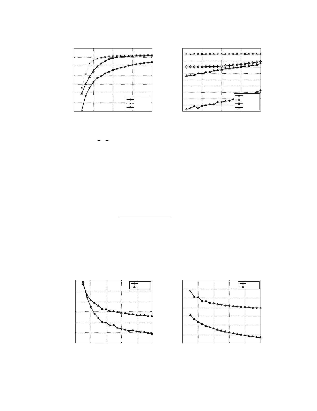
Authors: Edoardo M Airoldi, Thiago B Costa, Stanley H Chan
Stochastic blockm odel appr oximation of a graphon: Theory and consistent estimati on ∗ Edoardo M. Airoldi Dept. Statistics Harvard Uni versity Thiago B. Costa SEAS, and Dept. Statistics Harvard Uni versity Stanley H. Chan SEAS, and Dept. Statistics Harvard University Abstract Non-par ametric approa ches for analyzing n etwork da ta b ased on exch angeable graph models (E xGM) have recently gaine d in terest. The key object that defin es an ExGM is often referre d to as a graphon . This non-par ametric per spectiv e o n network mod eling poses ch allenging question s on h ow to make in ference on the grapho n underlying observed netw or k data. In this paper, we prop ose a computa- tionally ef ficient procedu re to estimate a graph on from a set of observed networks generated from it. This proce dure is based on a stoc hastic blockmod el app roxi- mation (SBA) of the g raphon . W e show that, b y app roximatin g the graph on with a stochastic block m odel, the g rapho n can be con sistently estimated, th at is, the estimation error vanishes as the size of the graph appro aches infinity . 1 Intr oduction Re vealing hid den structures o f a graph is the h eart of m any data ana lysis pro blems. From the well- known sma ll-world network to the r ecent large-scale data co llected from o nline service providers such as W ikipedia, T witter and F aceb ook, there is al ways a momentum in seekin g better an d more inform ativ e r epresentation s of th e graph s (Fienb erg et al. 1 985; Nowicki and Snijders 20 01a; Hoff et al. 200 2; Handco ck et al. 200 7; Airold i et al. 20 08; Xu et al. 20 12; Azari and Airo ldi 2 012; T ang et al. 2013; Goldenberg et al. 20 09; Kolaczyk 2009). In th is pap er , we d ev elo p a n ew com- putational tool to study one type of non-pa rametric represen tations wh ich recently draws sign ifi- cant atten tions fro m the com munity (Bickel and Chen 200 9; Lloyd et al. 2012; Bickel et al. 2011; Zhao et al. 2011; Orbanz and Roy 2013). The r oot of the non-p arametric model discussed in this pa per is in the theory of exchan ge- able random arrays (Aldous 1981; Hoover 1979; Kallenberg 1989), and it is presented in (Diaconis and Janson 2 008) as a link co nnecting de Finetti’ s w o rk o n p artial exchangeability and graph limits ( Lov ´ asz and Sze g edy 2 006; Borgs et al. 2006). I n a nutshe ll, the theory predicts that ev ery con vergent sequen ce of graphs ( G n ) h as a limit ob ject that preserves many local and global proper ties o f th e grap hs in th e sequen ce. Th is limit object, which is called a grapho n , can be rep- resented b y me asurable fu nctions w : [0 , 1] 2 → [0 , 1] , in a way that any w ′ obtained from m easure preserving transforma tions of w describes the same grap hon. Graphon s are usually seen as kernel fu nctions for ran dom n etwork mode ls (Lawrence 2 005). T o construct an n -vertex random graph G ( n, w ) for a giv en w , we first assign a rando m lab el u i ∼ Uniform [0 , 1] to ea ch vertex i ∈ { 1 , . . . , n } , and conn ect any two vertices i and j with prob ability w ( u i , u j ) , i.e. , Pr ( G [ i, j ] = 1 | u i , u j ) = w ( u i , u j ) , i, j = 1 , . . . , n , (1) where G [ i, j ] denotes the ( i, j ) th entry o f the adjacency matrix r epresenting a p articular r ealization of G ( n, w ) (See Figure 1). As an example, we note that the stochastic block-model is the case where w ( x, y ) is a piecewise constant function. ∗ This paper appears in the proceedings of NIPS 2013. In this version we include an appendix with proofs. 1 u i u j w × ( u i , u j ) w ( u i , u j ) G 1 G 2 T Figure 1: [Left] Given a grapho n w : [0 , 1] 2 → [0 , 1] , we draw i.i.d. samples u i , u j from Uniform[ 0,1] and assign G t [ i, j ] = 1 with prob ability w ( u i , u j ) , for t = 1 , . . . , 2 T . [Middle] Heat map of a g raphon w . [Right] A rando m graph gen erated by the gra phon shown in the middle . Rows and column s of the graph are ordered by increasing u i , instead of i for better visualization. The problem of interest is defined as follows: Given a sequence o f 2 T ob served dir ected gra phs G 1 , . . . , G 2 T , can we make an estimate b w of w , such that b w → w with high probability as n goes to infinity? This question has b een loo sely attempted in the literature, but none of which has a complete solution. For example, Lloyd et al. (Lloyd et al. 2 012) propo sed a Bayesian estimator withou t a consistency proof; Choi and W olfe (Choi and W olfe) stud ied the consistency properties, b ut d id not provide algo rithms to estimate the grapho n. T o the best of our knowledge, the only me thod tha t estimates gra phons consistently , besides ours, is USVT (Chatterjee). Howe ver, our alg orithm has better co mplexity and outper forms USVT in our simulations. More recently , oth er gr oups have begun e xp loring approaches related to ours (W olfe and Olhede 2013; P .Latouche and Robin 2013). The p roposed approxim ation pr ocedure req uires w to be piecewise Lipschitz. T he b asic idea is to approx imate w by a two-dimen sional step function b w with diminishing intervals as n in creases.The propo sed method is c alled the Stochastic blockmod el approx imation ( SB A) algor ithm, as the id ea of u sing a two-dimen sional step fun ction for appr oximation is equivalent to u sing the stochastic block mo dels ( Choi et al. 20 12; Nowicki and Snijders 2 001a; Hoff 20 08; Chann arond et al. 20 12; Rohe et al. 2011). Th e SBA algo rithm is defined up to pe rmutation s of th e nodes, so the estimated grapho n is not canonical. Howe ver , this doe s no t affect the con sistency prop erties of the SB A algorithm , as the consistency is measured w . r .t. th e graphon that generates the graphs. 2 Stochastic blockmodel approximation: Proced ure In this section we present the propo sed SB A algo rithm and discuss its basic properties. 2.1 Assumptions on graphons W e assume that w is piecewise Lipschitz , i.e. , there exists a seq uence o f no n-overlaping intervals I k = [ α k − 1 , α k ] defined by 0 = α 0 < . . . < α K = 1 , and a constant L > 0 such that, fo r any ( x 1 , y 1 ) and ( x 2 , y 2 ) ∈ I ij = I i × I j , | w ( x 1 , y 1 ) − w ( x 2 , y 2 ) | ≤ L ( | x 1 − x 2 | + | y 1 − y 2 | ) . For gene rality we assume w to be asym metric i.e. , w ( u, v ) 6 = w ( v , u ) , so that symmetric graph ons can be consider ed as a spe cial ca se. Consequ ently , a rando m graph G ( n, w ) g enerated by w is directed, i.e. , G [ i, j ] 6 = G [ j, i ] . 2.2 Similarity of graphon slices The intuitio n of the propo sed SB A algorith m is that if the g raphon is smoo th, neighborin g cro ss- sections of the graphon shou ld be similar . In other words, if two la bels u i and u j are close i.e. , 2 | u i − u j | ≈ 0 , then the difference between the ro w s lices | w ( u i , · ) − w ( u j , · ) | and the column slices | w ( · , u i ) − w ( · , u j ) | sho uld also be small. T o measure the similarity between two labels using th e grapho n s lices, we defin e the following distance d ij = 1 2 Z 1 0 [ w ( x, u i ) − w ( x, u j )] 2 dx + Z 1 0 [ w ( u i , y ) − w ( u j , y )] 2 dy . (2) Thus, d ij is small only if both row and column slices of the grap hon are similar . The usage of d ij for grapho n estimation will be discussed in the next sub section. But before we proceed, it should b e no ted th at in practice d ij has to b e estimated from the o bserved gra phs G 1 , . . . , G 2 T . T o deriv e an estimator b d ij of d ij , it is helpful to express d ij in a way that th e estima- tors can be easily obtained . T o this end, we let c ij = Z 1 0 w ( x, u i ) w ( x, u j ) dx and r ij = Z 1 0 w ( u i , y ) w ( u j , y ) dy , and expre ss d ij as d ij = 1 2 h ( c ii − c ij − c j i + c j j ) + ( r ii − r ij − r j i + r j j ) i . Inspecting this expression, we consider the following estimators for c ij and r ij : b c k ij = 1 T 2 X 1 ≤ t 1 ≤ T G t 1 [ k , i ] X T 0 . If b d i p ,i v < ∆ 2 , then we assign i v to the sam e block as i p . Therefor e, after scan ning thr ough Ω on ce, a block b B 1 = { i p , i v 1 , i v 2 , . . . } will be defined . By u pdating Ω as Ω ← Ω \ b B 1 , the process repeats until Ω = ∅ . The proposed greedy algorithm is only a local solution in a sense that it does not return the globally optimal clusters. Howe ver, as will b e shown in Sectio n 3, altho ugh the clustering algor ithm is not globally optimal, the e stimated grap hon b w is still guaranteed to b e a co nsistent estimate of th e tru e grapho n w as n → ∞ . Since th e gre edy algorithm is numerically efficient, it serves as a practical computatio nal tool to estimate w . 2.4 Main algorithm Algorithm 1 Stochastic blockmo del approximation Input: A set of observed graphs G 1 , . . . , G 2 T and the precision parameter ∆ . Output: Estimated stochastic blocks b B 1 , . . . , b B K . Initialize: Ω = { 1 , . . . , n } , and k = 1 . while Ω 6 = ∅ do Randomly choose a vertex i p from Ω and assign it as the piv ot for b B k : b B k ← i p . for Every other vertices i v ∈ Ω \{ i p } do Compute the distance estimate b d i p ,i v . If b d i p ,i v ≤ ∆ 2 , then assign i v as a member of b B k : b B k ← i v . end for Update Ω : Ω ← Ω \ b B k . Update counte r: k ← k + 1 . end while Algorithm 1 illu strates th e p seudo-co de for the p roposed stochastic block-m odel approx imation. The complexity of this alg orithm is O ( T S K n ) , where T is half the numb er of observations, S is the size of the neighbo rhood , K is the nu mber of blocks and n is numb er of vertices of the graph. 3 Stochastic blockmodel approximation: Theory of estimation In this section we pr esent the theoretical aspects of th e p roposed SB A algor ithm. W e will first discuss the p roperties of the estimator b d ij , and then show the con sistency of th e estimated gra phon b w . Details of the proof s can be found in the s u pplementa ry material. 3.1 Concentratio n analysis of b d ij Our first theorem belo w shows that the proposed estimator b d ij is both unbiased, and is concentrated around its expected v alue d ij . Theorem 1. The estimator b d ij for d ij is unbiased, i.e., E [ b d ij ] = d ij . Further , for any ǫ > 0 , Pr h b d ij − d ij > ǫ i ≤ 8 e − S ǫ 2 32 /T +8 ǫ/ 3 , (7) wher e S is the size of the neighb orhood S , and 2 T is the number of observations. Pr oof. He re we only highlight the importa nt steps to presen t the intuition. The basic idea of th e proof is to zoom-in a microscop ic term of b r k ij and show that it is unb iased. T o this end , we use the 4 fact that G t 1 [ i, k ] and G t 2 [ j, k ] ar e conditionally independ ent on u k to show E [ G t 1 [ i, k ] G t 2 [ j, k ] | u k ] = P r[ G t 1 [ i, k ] = 1 , G t 2 [ j, k ] = 1 | u k ] ( a ) = Pr[ G t 1 [ i, k ] = 1 | u k ] Pr[ G t 2 [ j, k ] = 1 | u k ] = w ( u i , u k ) w ( u j , u k ) , which then implies E [ b r k ij | u k ] = w ( u i , u k ) w ( u j , u k ) , and by iterated expectation we h av e E [ b r k ij ] = E [ E [ b r k ij | u k ]] = r ij . The concen tration in equality follo ws from a similar idea to bound th e v arianc e of b r k ij and apply Bernstein’ s inequality . That G t 1 [ i, k ] an d G t 2 [ j, k ] a re conditio nally indepen dent on u k is a critical fact fo r the success of the prop osed algo rithm. It als o explains why at least 2 independently observed graphs are necessary , for otherwise we canno t s ep arate the probab ility in the second equality above marked with ( a ) . 3.2 Choosing the number of blocks The performance of the Algo rithm 1 is sensiti ve to the number o f b locks it defines. On t h e one hand, it is desirab le to ha ve more block s so that the graph on can be finely approxima ted. But o n the other hand, if the number of blocks is too large then each block will contain only fe w vertices. This is bad because in order to estimate the value on each block, a suf ficient number of vertices i n each block is required . The trade- off b etween these two cases is controlled by the p recision paramete r ∆ : a large ∆ g enerates fe w large clusters, while small ∆ generates many small clusters. A precise relationship between the ∆ and K , the numb er of blocks generated the algorithm, is gi ven in Theorem 2. Theorem 2. Let ∆ be the a ccuracy p arameter and K be the numb er of blo cks estimated by Algo- rithm 1, then Pr " K > QL √ 2 ∆ # ≤ 8 n 2 e − S ∆ 4 128 /T + 16∆ 2 / 3 , (8) wher e L is the Lipschitz constan t and Q is the nu mber of Lipsc hitz b locks in w . In p ractice, we estimate ∆ using a cro ss-validation sche me to find the optimal 2D histogram b in width (W asserm an 2 005). The ide a is to test a seq uence of potential values o f ∆ and seek the one that minimizes the cross validation risk, defined as b J (∆) = 2 h ( n − 1 ) − n + 1 h ( n − 1 ) K X j =1 b p 2 j , (9) where b p j = | b B j | /n and h = 1 /K . Algorithm 2 details the prop osed cross-v alidatio n scheme. Algorithm 2 Cross V alidation Input: Graphs G 1 , . . . , G 2 T . Output: Blocks b B 1 , . . . , b B K , and optimal ∆ . for a sequence of ∆ ’ s do Estimate blocks b B 1 , . . . , b B K from G 1 , . . . , G 2 T . [Algorith m 1] Compute b p j = | b B j | /n , for j = 1 , . . . , K . Compute b J (∆) = 2 h ( n − 1) − n +1 h ( n − 1) P K j =1 b p 2 j , with h = 1 /K . end for Pick the ∆ with minimu m b J (∆) , and the correspond ing b B 1 , . . . , b B K . 3.3 Consistency of b w The goal o f our next theore m is to show that b w is a consistent esti m ate of w , i.e. , b w → w as n → ∞ . T o begin with, let us first recall two commonly used metric: 5 Definition 1. The mean squ ar ed err or (MSE) and mean absolute err or (MAE) ar e defi ned as MSE( b w ) = 1 n 2 n X i v =1 n X j v =1 ( w ( u i v , u j v ) − b w ( u i v , u j v )) 2 MAE( b w ) = 1 n 2 n X i v =1 n X j v =1 | w ( u i v , u j v ) − b w ( u i v , u j v ) | . Theorem 3. If S ∈ Θ( n ) and ∆ ∈ ω log( n ) n 1 4 ∩ o (1) , then lim n →∞ E [MAE( b w )] = 0 and lim n →∞ E [MSE( b w )] = 0 . Pr oof. T he d etails of the pro of can be fou nd in th e supplemen tary mate rial . Here we only outline the key steps to present the intuition of the theorem. Th e goal of Theorem 3 is to s how conv ergence of | b w ( u i , u j ) − w ( u i , u j ) | . The idea is to consider the following two quantities: w ( u i , u j ) = 1 | b B i | | b B j | X i x ∈ b B i X j x ∈ b B j w ( u i x , u j x ) , b w ( u i , u j ) = 1 | b B i | | b B j | X i x ∈ b B i X j y ∈ b B j 1 2 T ( G 1 [ i x , j y ] + G 2 [ i x , j y ] + . . . + G 2 T [ i x , j y ]) , so that if we can boun d | w ( u i , u j ) − w ( u i , u j ) | an d | w ( u i , u j ) − b w ( u i , u j ) | , the n consequ ently | b w ( u i , u j ) − w ( u i , u j ) | can also be bou nded. The bou nd for the first term | w ( u i , u j ) − w ( u i , u j ) | is shown in Lemma 1: By Algorithm 1, any vertex i v ∈ b B i is g uaranteed to b e with in a d istance ∆ from th e piv ot of b B i . Since w ( u i , u j ) is an av era ge ov er b B i and b B j , by Theorem 1 a probability bound in volving ∆ can be ob tained. The bo und for the seco nd term | w ( u i , u j ) − b w ( u i , u j ) | is s h own in Lemma 2. Different f rom Lemm a 1, here we need to consider tw o possible situa tions: eith er the intermediate estimate w ( u i , u j ) is close to the ground truth w ( u i , u j ) , or w ( u i , u j ) is far from the gro und truth w ( u i , u j ) . This ac- counts for the sum in Lemma 2. Individual boun ds are deri ved based on Lemma 1 and Theorem 1. Combining Lemma 1 and Lemma 2, we can then bound the error and show con vergence. Lemma 1. F or any i v ∈ b B i and j v ∈ b B j , Pr h | w ( u i , u j ) − w ( u i v , u j v ) | > 8∆ 1 / 2 L 1 / 4 i ≤ 32 | b B i | | b B j | e − S ∆ 4 32 /T + 8∆ 2 / 3 . (10) Lemma 2. F or any i v ∈ b B i and j v ∈ b B j , Pr h | b w ij − w ij | > 8∆ 1 / 2 L 1 / 4 i ≤ 2 e − 256( T | b B i | | b B j | √ L ∆) + 32 | b B i | 2 | b B j | 2 e − S ∆ 4 32 /T + 8∆ 2 / 3) . (11) The condition S ∈ Θ( n ) is necessary to make Theor em 3 v alid, becau se if S is in depend ent of n , it is not possible to drive (1 0) an d ( 11) to 0 even if n → ∞ . The other condition on ∆ is also importan t as it forces the n umerator s and d enomin ators in the exponentials o f ( 10) a nd (11) to be well behav ed . 4 Experiments In th is section we ev aluate the proposed SBA algorith m by showing some empirical results. For the purp ose of compariso n, we c onsider (i) the un iv ersal singular value thresholdin g (USVT) (Chatterjee); (ii) th e largest-gap algorithm (LG) (Chan narond et al. 2012); (iii) matrix c ompletion from few entries (OptSpace) (Kesha van et al. 2010). 6 4.1 Estimating stochastic blockmodels Accuracy as a function of growing graph size. Our first experim ent is to evaluate the propo sed SB A algorith m for estimating sto chastic blockm odels. For th is pur pose, we ge nerate (ar bitrarily) a grapho n w = 0 . 8 0 . 9 0 . 4 0 . 5 0 . 1 0 . 6 0 . 3 0 . 2 0 . 3 0 . 2 0 . 8 0 . 3 0 . 4 0 . 1 0 . 2 0 . 9 , (12) which represen ts a piecewise constant function with 4 × 4 e qui-space blocks. 0 200 400 600 800 1000 −3 −2.5 −2 −1.5 −1 −0.5 n log 10 (MAE) Proposed Largest Gap OptSpace USVT 0 5 10 15 20 25 30 35 40 −3 −2.9 −2.8 −2.7 −2.6 −2.5 −2.4 −2.3 −2.2 −2.1 −2 2 T log 10 (MAE) Proposed (a) Growing graph size, n (b) Growing no. observations, 2 T Figure 2: (a) MAE reduce s as grap h size g rows. For the fairne ss of the am ount o f d ata that can be used, we use n 2 × n 2 × 2 observations for SB A, and n × n × 1 observation for USVT (Chatterjee) and LG (Channarond et al. 2012). ( b) MAE of th e proposed SB A algorithm reduces when more observations T is avail ab le. Both plots are a veraged over 100 independent trials. Since USVT and LG use on ly one observed graph whereas the pro posed SB A re quire at least 2 observations, in order to make the compar ison fair , we use half of the n odes for SBA by gener ating two independent n 2 × n 2 observed graphs. For USVT and LG, we use one n × n o bserved graph. Figure 2(a) shows the asymp totic b ehavior of the algor ithms when n grows. Figur e 2(b) shows the estimation error of SB A algor ithm as T gr ows for graphs of size 200 vertices. Accuracy as a function of growing number of blocks. Our second experiment is to ev aluate the perfor mance of the a lgorithms as K , the number of block s, increases. T o this end , we c onsider a sequence of K , and for ea ch K we generate a grapho n w of K × K b locks. Each e ntry of the block is a random n umber generated fro m Un iform [0 , 1] . Same a s the previous experim ent, we fix n = 2 00 and T = 1 . T he experimen t is r epeated over 1 00 trials so that in every trial a different grapho n is generated. Th e result s h own in Figure 3(a) i n dicates that while estimation error incre ases as K grows, the proposed SB A algorithm still attains the lowest MAE for all K . 4.2 Estimation with missing edges Our next experim ent is to ev aluate the perf ormance of prop osed SB A alg orithm when there are missing edges in the observed graph. T o model missing edges, we construct an n × n binary matrix M with pro bability Pr[ M [ i, j ] = 0] = ξ , where 0 ≤ ξ ≤ 1 define s the percentag e of m issing edges. Giv en ξ , 2 T matrices are g enerated with missing edges, and the observed graphs are defined as M 1 ⊙ G 1 , . . . , M 2 T ⊙ G 2 T , where ⊙ denotes the element-wise multip lication. T he goal is to study how well SB A can reco nstruct the graphon b w in the presence of missing links. The mod ification of the prop osed SB A algor ithm for the case missing links is m inimal: when com - puting (6 ) , instead of a veraging over all i x ∈ b B i and j y ∈ b B j , we only av era ge i x ∈ b B i and j y ∈ b B j that are not m asked out b y all M ′ s. Figu re 3(b) shows th e result of average over 10 0 indep endent 7 0 5 10 15 20 −1.4 −1.3 −1.2 −1.1 −1 −0.9 −0.8 −0.7 K log 10 (MAE) Proposed Largest Gap USVT 0 5 10 15 20 −1.6 −1.5 −1.4 −1.3 −1.2 −1.1 −1 −0.9 −0.8 −0.7 −0.6 % mi ssi ng links log 10 (MAE) Proposed Largest Gap OptSpace USVT (a) Growing no. blo cks, K (b) Missing links Figure 3: (a) As K increases, M AE of all thr ee algor ithm increases but SB A still a ttains the lowest MAE. Here, we use n 2 × n 2 × 2 ob servations for SB A, and n × n × 1 observation for USVT (Chatterjee) and L G (Channa rond et al. 2012). (b) Estimation of gr aphon in th e p resence of missing links: As the amount of missing links increases, estimation error also increases. trials. Here, we consider the graphon given in (12), with n = 2 00 and T = 1 . It is evident that SB A outperf orms its counterparts at a lower rate of missing links. 4.3 Estimating continuous graphons Our final experiment is to e valuate the proposed SB A algor ithm in estimating continuous graphons. Here, we consider two of the graphon s reported in (Chatterjee): w 1 ( u, v ) = 1 1 + exp {− 50( u 2 + v 2 ) } , and w 2 ( u, v ) = u v , where u, v ∈ [0 , 1 ] . Her e, w 2 can be consid ered as a special case of the Eig enmodel (Hoff 2008) or latent feature relational model (Miller et al. 2009). The results in Figure 4 shows that while b oth algorithms have impr oved estimates when n g rows, the perfor mance depen ds o n which o f w 1 and w 2 that we are studying . This suggests that in practice the choice o f the algor ithm should d epend on th e expected structur e of the gr aphon to be estimated: I f the graph generated by the g rapho n demonstrates som e low-rank proper ties, then USVT is likely to be a better option. For more structured or complex grapho ns the proposed procedure is recommended. 0 200 400 600 800 1000 −3.2 −3.15 −3.1 −3.05 −3 −2.95 −2.9 n log 10 (MAE) Proposed USVT 0 200 400 600 800 1000 −2 −1.8 −1.6 −1.4 −1.2 −1 −0.8 −0.6 n log 10 (MAE) Proposed USVT (a) grapho n w 1 (b) graphon w 2 Figure 4: Co mparison between SB A and USVT in estimatin g two continuou s graphons w 1 and w 2 . Evidently , SB A performs better for w 1 (high- rank) and worse for w 2 (low-rank). 8 5 Concluding re marks W e presen ted a new co mputatio nal to ol fo r estimating graph ons. The pro posed algorithm approx- imates the con tinuous grapho n by a sto chastic block -mod el, in which th e fir st step is to clu ster the un known vertex labels into blo cks by using an emp irical estimate of the distance between two grapho n slices, and the second step is to build an empirical histogram to estimate the gra phon. Com- plete consistency analysis of the algorithm is der iv ed. Th e algorithm was ev aluated experimen tally , and we found that the algorithm is effecti ve in estimating block structured graphons. Code . An implementatio n o f the sto chastic blo ckmod el appro ximation ( SB A) alg orithm p roposed in this paper is a vailable online at: https://gith ub.com/airol dilab/SBA Acknowledgments . EMA is partially supported by NSF CAREER award IIS-11 4966 2, ARO MURI award W911NF-1 1-1-0 036, and an Alfred P . Sloan R esear ch Fellowship. SHC is partially supp orted by a Croucher Foundation Post-Doctoral Research Fello wship. Refer ences E.M. Airoldi, D.M. Blei, S.E. Fienbe rg, and E.P . Xing. Mixe d-membership stochastic blockmodels. Journa l of Mach ine Learning Resear ch , 9:1981–201 4, 2008. D.J. Aldous. Representations for partially exc hangeable arrays of random variab les. Journal of Multivariate Analysis , 11:581–59 8, 1981. H. Azari and E. M. Airoldi. Graphlet decomposition of a weighted netwo rk. Journ al of Machine Learning Resear ch, W&CP , 22:54–63, 2012. P .J. Bickel and A. Chen. A non parametric vie w of network models and Newman -Gir v an and other mod ulariti es. Pr oc. Natl. Acad. Sci. USA , 106:21068 –21073, 2009. P .J. Bickel, A. Chen, and E. Levina. The method of moments and degree distributions for network models. Annals of Statistics , 39(5):2280 –2301, 2011. C. Borgs, J. Chayes, L. Lov ´ asz, V . T . S ´ os, B . Szegedy , and K. V esztergombi. Graph li mits and parameter testing. In Proc. ACM Sy mposium on Theory of Computing , pages 261–270, 2006. A. Channarond, J. Daudin, and S . Robin. Classification and estimation in the Stochastic Blockmodel based on the empirical degrees. Electr onic Jo urnal of Statistics , 6:2574–26 01, 2012. S. Chatterjee. Matrix estimation by univ ersal singular v alue thresholding. ArXiv:1212.124 7. 2012. D.S. Choi and P .J. W olfe. Co-clustering separately exch angeable network data. ArXiv:1212.4 093. 2012. D.S. Choi, P .J. W olfe, and E.M. Airoldi. Stochastic blockmodels with a gro wing nu mber o f classes. Biometrika , 99:273–2 84, 2012. P . Diaconis and S. Janson. Graph limits and exchangeab le random graphs. Rendiconti di Matematica e delle sue Applicazioni, Series VII , pages 33–61 , 2008. S. E. Fienb erg, M. M. Me yer , and S. W asserman. Statistical analysis of multiple sociometric relations. Jou rnal of the American Statistical Association , 80:51–67, 1985. A. Golden berg, A.X. Zheng, S.E. Fienb erg, and E.M. Airoldi. A survey of statistical netwo rk models. F ounda- tions and T r ends in Machine Learning , 2:129– 233, 2009. M. Handcock, A. E. Raftery , and J. T antrum. Model-base d clustering for social network s (with discussion). J ournal of t he Royal Statistical Society , Series A , 170:301 –354, 2007. P .D. Hoff. Modeling homo phily and stocha sti c eq uiv alence in symmetric relational data. I n Neural I nformation Pr ocessing Systems (NIPS) , volume 20, pages 657– 664, 2008. P .D. Hoff, A.E. Raftery , and M.S. Handcock. Latent space approaches to social network analysis. Journa l of the American Statistical Association , 97(460):109 0–1098, 2002. D.N. Hoov er . Relations on probability spaces and arrays of random variables. Pr eprint, Institute for Advanced Study , Princeton, NJ , 1979. O. Kall enberg . On the representation theorem for exchan geable arrays. Jour nal of Multivariate Analysis , 30 (1):137–154 , 1989. R.H. Keshav an, A. Montanari, and S. Oh. Matrix completion from a fe w entries. IEEE Tr ans. Information Theory , 56:2980– 2998, Jun. 2010. E. D. K olaczyk. Statistical Analysis of Network Data: Methods and Models . Springer , 2009. 9 N.D. Lawrence. Probabilistic non-linear principal component analysis wit h Gaussian process latent variable models. Jou rnal of Machine Learning Resear ch , 6:1783–18 16, 2005. J.R. Lloyd, P . Orbanz, Z. Ghahramani, and D.M. Roy . Random function priors for exchangeab le arrays with applications to graphs and relational data. In Neural Information Pr ocessing Systems (NIPS) , 2012. L. L ov ´ asz and B. Szegedy . Limi ts of dense graph sequences. J ournal of Combinatorial Theory , Series B , 96: 933–95 7, 2006. K.T . Miller , T .L. Griffiths, and M.I. Jordan. Nonparametric l atent fature models for l ink prediction. I n N eural Information Pr ocessing Systems (NIPS) , 2009. K. No wicki and T . A. B. Snijders. Esti mation and prediction for stochastic blockstructures. Journ al of the American Statistical Association , 96:1077– 1087, 2001. P . Orbanz and D. M. Roy . B ayesian models of graphs, arrays and other exchangeable random structures, 2013. Unpublished manuscript. P .Latouche and S. Robin. Bay esian mod el a veraging of stochastic block models to estimate the graphon f unction and motif frequencies in a w-graph model. ArXiv:1310.61 50, October 2013. Unpub lished manuscript. K. Rohe, S . Chatterjee, and B. Y u. S pectral clus teri ng and the h igh-dimensional stochastic blockm odel. Annals of Statistics , 39(4):1878 –1915, 2011. M. T ang, D.L . Sussman, and C.E. Pri ebe. Univ ersally consistent vertex classification for latent positions graphs. Annals of Statistics , 2013. In press. L. W asse rman. All of Nonpar ametric Statistics . Springer , 2005. P .J. W olfe and S .C. Olhede. Nonpara metric graphon estimation. ArXi v:1309.5936 , S eptember 2013. Unpub - lished manuscript. Z. Xu, F . Y an, and Y . Qi. Infinite Tuck er decomposition: nonparametric Bayesian models for multiway data analysis. In Pro c. I ntl. Conf. M achine Learning (ICML) , 2012. Y . Zhao, E. L ev ina, and J. Zhu. Community extraction for social network s. In Proc. Natl. Acad. Sci. U SA , volume 1 08, pages 7321–7326 , 2011. A Proofs f or Section 3.1 Theorem 1. T he estimator b d ij for d ij is unbiased. Further , for any ǫ > 0 , if the gra ph is dir ected, then Pr h b d ij − d ij > ǫ i ≤ 8 e − S ǫ 2 32 /T + 8 ǫ/ 3 , (13) and if the grap h is un-dir ected, then Pr h b d ij − d ij > ǫ i ≤ 8 e − S ǫ 2 64 /T + 8 ǫ/ 3 , (14) wher e S is the size of the sampling neighborhood S , and 2 T is the number of observations. Pr oof. F irst, for gi ven u i and u j , let us define the following tw o quantities c ij def = Z 1 0 w ( x, u i ) w ( x, u j ) dx, r ij def = Z 1 0 w ( u i , y ) w ( u j , y ) dy . Consequently , we express d ij as d ij def = 1 2 Z 1 0 ( w ( u i , y ) − w ( u j , y )) 2 dy + Z 1 0 ( w ( x, u i ) − w ( x, u j )) 2 dx = 1 2 [( r ii − r ij − r j i + r j j ) + ( c ii − c ij − c j i + c j j )] . In order to study b d ij (the estimator of d ij ), it is desired to exp ress b d ij in the same form of d ij : b d ij = 1 S X k ∈S 1 2 h b r k ii − b r k ij − b r k j i + b r k j j + b c k ii − b c k ij − b c k j i + b c k j j i , (15) 10 where S = { 1 , . . . , n }\{ i, j } is t he sampling neighborho od, and S = |S | . I n (15), indi vidual components are defined as b c k ij = 1 T 2 X 1 ≤ t 1 ≤ T G t 1 [ k, i ] X T ǫ = Pr " 1 S X k ∈S 1 2 b r k ij + b c k ij − 1 2 ( r ij + c ij ) > ǫ # ≤ 2 e − S ǫ 2 2 ( V ar [ 1 2 ( b r k ij + b c k ij )] + ǫ/ 3 ) ≤ 2 e − S ǫ 2 2(1 /T + ǫ/ 3) . Finally , we note that | b d ij − d ij | ≤ 1 2 | b r ii + b c ii − r ii − c ii | + 1 2 | b r ij + b c ij − r ij − c ij | + 1 2 | b r j i + b c j i − r j i − c j i | + 1 2 | b r j j + b c j j − r j j − c j j | . Therefore by union bound we hav e Pr[ | b d ij − d ij | > ǫ ] ≤ Pr h 1 2 | b r ii + b c ii − r ii − c ii | + 1 2 | b r ij + b c ij − r ij − c ij | + + 1 2 | b r j i + b c j i − r j i − c j i | + 1 2 | b r j j + b c j j − r j j − c j j | > ǫ i ≤ Pr h 1 2 ( b r ii + b c ii ) − 1 2 ( r ii + c ii ) > ǫ/ 4 i + Pr h 1 2 ( b r ij + b c ij ) − 1 2 ( r ij + c ij ) > ǫ/ 4 i + + Pr h 1 2 ( b r j i + b c j i ) − 1 2 ( r j i + c j i ) > ǫ/ 4 i + Pr h 1 2 ( b r j j + b c j j ) − 1 2 ( r j j + c j j ) > ǫ/ 4 i ≤ 8 e − S ǫ 2 / 16 2(1 /T + ǫ/ 12) = 8 e − S ǫ 2 32 /T + 8 ǫ/ 3 . If the g raph is un-directed, t hen c k ij = r k ij and we ca n only have V ar 1 2 r k ij + c k ij ≤ 2 T instead of V ar 1 2 r k ij + c k ij ≤ 1 T . In this case, Pr[ | b d ij − d ij | > ǫ ] ≤ 8 e − S ǫ 2 64 /T + 8 ǫ/ 3 . B Proofs f or Section 3.2 Theorem 2. L et ∆ be the accurac y parameter and K be t he number of bloc ks estimated by Algorithm 1, then Pr K > QL √ 2 ∆ ≤ 8 n 2 e − S ∆ 4 128 /T + 16∆ 2 / 3 , (21) wher e L is the L ipschitz co nstant and Q is the number of L ipschitz b locks in the gr ound truth w . Pr oof. R ecall that in defining the L ipschitz condition of w (S ection 2.1), we defined a sequence of non- ov erlapping intervals I k = [ α k , α k +1 ] , where 0 = α 0 < . . . < α Q = 1 , and Q is t he number of Lipschitz blocks of w . For each of the interv al I k , we divid e it into R def = L √ 2 ∆ subinterv als of equal size 1 /R . Thus, the distance between any two elements in the same subinterv al is at most 1 /R . Also, the total number of subinterv als ov er [0 , 1] is QR . No w , suppose that there are K > QR = QL √ 2 ∆ blocks defined by t he algorithm, and denote the K piv ots be p 1 , . . . , p K . By the pigeonhole principle, there must be at least two pi vots p i and p j in the same sub-interval. In this case, the distance d p i ,p j must satisfy the following c ondition: d p i ,p j = 1 2 Z 1 0 ( w ( x, u p i ) − w ( x, u p j )) 2 dx + Z 1 0 ( w ( u p i , y ) − w ( u p j , y )) 2 dy ≤ L 2 ( u p i − u p j ) 2 ≤ L 2 1 R 2 = ∆ 2 2 . Ho wever , from the algorithm it holds that b d p i ,p j ≥ ∆ 2 . So, if K > Q R , then b d p i ,p j − d p i ,p j > ∆ 2 2 . 13 Let E be the follo wing even t: E = b d p i ,p j − d p i ,p j > ∆ 2 2 for at least one pair of p i , p j . Then, since the e vent E is a consequence of the ev ent { K > QR } , we have Pr K > QL √ 2 ∆ = Pr[ K > QR ] ≤ Pr[ E ] . T o b ound Pr[ E ] , we observ e that Pr b d p i ,p j − d p i ,p j > ∆ 2 2 p i , p j ≤ 8 e − S (∆ 2 / 2) 2 32 /T + 8(∆ 2 / 2) / 3 = 8 e − S ∆ 4 128 /T + 16∆ 2 / 3 . Therefore, by union bound, Pr h E p 1 , . . . , p K i ≤ X p i ,p j Pr b d p i ,p j − d p i ,p j > ∆ 2 2 p i , p j ≤ 8 n 2 e − S ∆ 4 128 /T + 16∆ 2 / 3 , and hence, Pr [ E ] = X p 1 ,...,p K Pr [ E | p 1 , . . . , p K ] Pr [ p 1 , . . . , p K ] ≤ 8 n 2 e − S ∆ 4 128 /T + 16∆ 2 / 3 · X p 1 ,...,p K Pr [ p 1 , . . . , p K ] = 8 n 2 e − S ∆ 4 128 /T + 16∆ 2 / 3 . This completes the proof. C Proofs f or Section 3.3 Lemma 1. Let b B i = { i 1 , i 2 , . . . , i | b B i | } and b B j = { j 1 , j 2 , . . . , j | b B j | } be two clusters r eturned by the Al- gorithm. Suppose t hat { u i 1 , u i 2 , . . . , u i | b B i | } and { u j 1 , u j 2 , . . . , u j | b B j | } ar e the gr ound t ruth labels of the vertices in b B i and b B j , r espectively . L et w ij = 1 | b B i || b B j | X i x ∈ b B i X j x ∈ b B j w ( u i x , u j x ) . (22) Assume that the pr ecision parameter satisfies ∆ 2 < δ 2 L 4 , wher e L is the L ipschitz constan t and δ is the size of the smallest Lipschitz interval. Then, for any i v ∈ b B i and j v ∈ b B j , Pr h | w ij − w ( u i v ,j v ) | > 8∆ 1 / 2 L 1 / 4 i ≤ 32 | b B i || b B j | e − S ∆ 4 32 /T + 8∆ 2 / 3 . (23) Pr oof. L et i p ∈ b B i and j p ∈ b B j be piv ots of the clusters b B i and b B j , respectively . By definition of pi vots, it holds that | b d i p ,i v | ≤ ∆ 2 and | b d j p ,j v | ≤ ∆ 2 for an y vertices i v ∈ b B i and j v ∈ b B j . Therefore, 0 ≤ −| b d i p ,i v | + ∆ 2 ≤ − b d i p ,i v + ∆ 2 ⇒ d i p ,i v ≤ d i p ,i v − b d i p ,i v + ∆ 2 ≤ | d i p ,i v − b d i p ,i v | + ∆ 2 , which implies that Pr d i p ,i v > 2∆ 2 ≤ Pr h | d i p ,i v − b d i p ,i v | + ∆ 2 > 2∆ 2 i = Pr h | d i p ,i v − b d i p ,i v | > ∆ 2 i ≤ 8 e − S ∆ 4 32 /T +8∆ 2 / 3 . 14 Similarly , we ha ve Pr d j p ,j v > 2∆ 2 ≤ 8 e − S ∆ 4 32 /T + 8∆ 2 / 3 . Thus, Pr d i p ,i v > 2∆ 2 ∪ d j p ,j v > 2∆ 2 ≤ Pr d i p ,i v > 2∆ 2 + Pr d j p ,j v > 2∆ 2 ≤ 16 e − S ∆ 4 32 /T + 8∆ 2 / 3 . Let d c ij = R 1 0 ( w ( x, u i ) − w ( x, u j )) 2 dx and d r ij = R 1 0 ( w ( u i , y ) − w ( u j , y )) 2 dy . By Lemma 5, it holds that for any 0 < ( ǫ/ 2) 2 < 2 δ L , if d c i,j ≤ ( ǫ/ 2) 4 8 L = ǫ 4 128 L and d r i,j ≤ ǫ 4 128 L , then sup x ∈ [0 , 1] | w ( x , u i ) − w ( x, u j ) | ≤ ǫ 2 , sup y ∈ [0 , 1] | w ( u i , y ) − w ( u j , y ) | ≤ ǫ 2 . Therefore, if d c i p ,i v ≤ ǫ 4 128 L , d r i p ,i v ≤ ǫ 4 128 L , d c j p ,j v ≤ ǫ 4 128 L and d r j p ,j v ≤ ǫ 4 128 L , then for pivots i p ∈ b B i , j p ∈ b B j , and verte x i v ∈ b B i , j v ∈ b B j : | w ( u i v , u j v ) − w ( u i p , u j p ) | ≤ | w ( u i v , u j v ) − w ( u i v , u j p ) | + | w ( u i v , u j p ) − w ( u i p , u j p ) | ≤ su p x ∈ [0 , 1] | w ( x , u j v ) − w ( x, u j p ) | + sup y ∈ [0 , 1] | w ( u i v , y ) − w ( u j p , y ) | = ǫ 2 + ǫ 2 = ǫ. (24) Also, if d c i p ,i x ≤ ǫ 4 128 L , d r i p ,i x ≤ ǫ 4 128 L , d c j p ,j x ≤ ǫ 4 128 L and d r j p ,j x ≤ ǫ 4 128 L for verte x every i x ∈ b B i , j x ∈ b B j 1 | b B i || b B j | X i x ∈ b B i X j x ∈ b B j w ( u i x , u j x ) − w ( u i p , u j p ) ≤ 1 | b B i || b B j | X i x ∈ b B i X j x ∈ b B j w ( u i x , u j x ) − 1 | b B i | X i x ∈ b B i w ( u i x , u j p ) + 1 | b B i | X i x ∈ b B i w ( u i x , u j p ) − w ( u i p , u j p ) ≤ 1 | b B i | 1 | b B j | X i x ∈ b B i X j x ∈ b B j w ( u i x , u j x ) − w ( u i x , u j p ) + 1 | b B i | X i x ∈ b B i w ( u i x , u j p ) − w ( u i p , u j p ) ≤ 1 | b B i | 1 | b B j | X i x ∈ b B i X j x ∈ b B j ǫ 2 + 1 | b B i | X i x ∈ b B i ǫ 2 = ǫ. (25) Combining (24) and (25) with triangle inequality yields 1 | b B i || b B j | X i x ∈ b B i X j x ∈ b B j w ( u i x , u j x ) − w ( u i v , u j v ) ≤ 2 ǫ. Consequently , by contrapositiv e this implies that | w ij − w ( u i v , u j v ) | > 2 ǫ ⇒ [ i x ∈ b B i ,j x ∈ b B j d c i p ,i x > ǫ 4 128 L ∪ d r i p ,i x > ǫ 4 128 L ∪ d c j p ,j x > ǫ 4 128 L ∪ d r j p ,j x > ǫ 4 128 L ⇒ [ i x ∈ b B i ,j x ∈ b B j d i p ,i x > ǫ 4 128 L ∪ d j p ,j x > ǫ 4 128 L . Therefore, Pr [ | w ij − w ( u i v , u j v ) | > 2 ǫ ] ≤ Pr [ i x ∈ b B i ,j x ∈ b B j d i p ,i x > ǫ 4 128 L ∪ d j p ,j x > ǫ 4 128 L ≤ X i x ∈ b B i ,j x ∈ b B j Pr d i p ,i x > ǫ 4 128 L + Pr d j p ,j x > ǫ 4 128 L . 15 Assuming ∆ < δ √ L/ 2 and setting ǫ = 4∆ 1 / 2 L 1 / 4 , we hav e 0 < ( ǫ/ 2) 2 < 2 δ L and thus Pr h | w ij − w ( u i v , u j v ) | > 8∆ 1 / 2 L 1 / 4 i ≤ X i x ∈ b B i ,j x ∈ b B j Pr d i p ,i x > 2∆ 2 + Pr d j p ,j x > 2∆ 2 ≤ 32 | b B i || b B j | e − S ∆ 4 32 /T +8∆ 2 / 3 . Lemma 2. Let b B i = { i 1 , i 2 , . . . , i | b B i | } and b B j = { j 1 , j 2 , . . . , j | b B j | } be two clusters r eturned by the Al- gorithm. Suppose t hat { u i 1 , u i 2 , . . . , u i | b B i | } and { u j 1 , u j 2 , . . . , u j | b B j | } ar e the gr ound t ruth labels of the vertices in b B i and b B j , r espectively . L et b w ij = 1 | b B i || b B j | X i x ∈ b B i X j x ∈ b B j G 1 [ i x , j x ] + . . . + G 2 T [ i x , j x ] 2 T , w ij = 1 | b B i || b B j | X i x ∈ b B i X j x ∈ b B j w ( u i x , u j x ) . Then, Pr h | b w ij − w ij | > 8∆ 1 / 2 L 1 / 4 i ≤ 2 e − 256( T | b B i | | b B j | √ L ∆) + 32 | b B i | 2 | b B j | 2 e − S ∆ 4 32 /T + 8∆ 2 / 3 . Pr oof. T here are two possible situations that we need to consider . Case 1 : For an y vertex i v ∈ b B i and j v ∈ b B j , the estimate of the p revious lemma w ij (independen t of ( i v , j v ) ) is close to the ground truth w ij def = w ( u i v , u j v ) . In other words, we w ant w ( u i v , u j v ) to stay close f or all i v ∈ b B i and j v ∈ b B j , so that the dif ference | w ij − w ij | remains small for all i v ∈ b B i and j v ∈ b B j . Case 2 : Complement of case 1. T o en capsulate these two cases, we first define the ev ent E = n | w ij − w ij | ≤ 8∆ 1 / 2 L 1 / 4 , ∀ i v ∈ b B i , j v ∈ b B j o and define E be the complemen t of E . Then, Pr h | b w ij − w ij | > 8∆ 1 / 2 L 1 / 4 i = Pr h | b w ij − w ij | > 8∆ 1 / 2 L 1 / 4 E i Pr [ E ] + Pr h | b w ij − w ij | > 8∆ 1 / 2 L 1 / 4 E i Pr E ≤ Pr h | b w ij − w ij | > 8∆ 1 / 2 L 1 / 4 E i + Pr E . So it remains to bound the two proba bilit ies. Conditioning on E , it holds that w ij − ǫ ≤ w ij ≤ w + ǫ. Fix a vertex pair ( i v , j v ) , we note that G 1 [ i v , j v ] , . . . , G 2 T [ i v , j v ] are independent Bernoulli r andom variable with common mean w ( u i v , u j v ) . Denote b w ij = 1 2 T | b B i || b B j | 2 T X t =1 X i x ∈ b B i X j x ∈ b B j G t [ i x , j x ] , then by Hoef fding inequality we hav e Pr h b w ij − w ij > 2 ǫ E i = Pr h b w ij > w ij + 2 ǫ E i ≤ Pr h b w ij > w ij + ǫ E i ≤ e − 2(2 T | b B i || b B j | ǫ 2 ) , and similarly Pr h b w ij − w ij < − 2 ǫ E i ≤ e − 2(2 T | b B i | | b B j | ǫ 2 ) . Therefore, Pr h | b w ij − w ij | > 2 ǫ E i ≤ 2 e − 2(2 T | b B i | | b B j | ǫ 2 ) . 16 Substituting ǫ = 4∆ 1 / 2 L 1 / 4 , we hav e Pr h | b w ij − w ij | > 8∆ 1 / 2 L 1 / 4 E i ≤ 2 e − 128( | b B i | | b B j | (2 T ) √ L ∆) . The second p robability is bounded as follo ws. Since E is the comp lement of E , it is bound ed by the probab il ity where at least one ( i v , j v ) violates the condition. Therefore, Pr E = Pr h at least one i v , j v s.t. | w ( u i v , u j v ) − w ij | > 8∆ 1 / 2 L 1 / 4 i ≤ X i v ∈ b B i X j v ∈ b B j Pr h | w ( u i v , u j v ) − w ij | > 8∆ 1 / 2 L 1 / 4 i ≤ 32 | b B i | 2 | b B j | 2 e − S ∆ 4 32 /T + 8∆ 2 / 3 . Finally , by combining the abo ve results we hav e Pr h | b w ij − w ij | > 8∆ 1 / 2 L 1 / 4 i ≤ 2 e − 256( T | b B i | | b B j | √ L ∆) + 32 | b B i | 2 | b B j | 2 e − S ∆ 4 32 /T + 8∆ 2 / 3 . Lemma 3. Let b B i = { i 1 , i 2 , . . . , i | b B i | } and b B j = { j 1 , j 2 , . . . , j | b B j | } be two clusters r eturned by the Al- gorithm. Suppose t hat { u i 1 , u i 2 , . . . , u i | b B i | } and { u j 1 , u j 2 , . . . , u j | b B j | } ar e the gr ound t ruth labels of the vertices in b B i and b B j , r espectively . L et b w ij = 1 | b B i || b B j | X i x ∈ b B i X j x ∈ b B j G 1 [ i x , j x ] + . . . + G 2 T [ i x , j x ] 2 T . Then, Pr h | b w ij − w ij | > 16∆ 1 / 2 L 1 / 4 i ≤ 2 e − 256( T | b B i | | b B j | √ L ∆) + 64 n 4 e − S ∆ 4 32 /T + 8∆ 2 / 3 . Pr oof. B y Lemma 1 and Lemma 2, we hav e Pr h | b w ij − w ij | > 8∆ 1 / 2 L 1 / 4 i ≤ 2 e − 256( T | b B i | | b B j | √ L ∆) + 32 | b B i | 2 | b B j | 2 e − S ∆ 4 32 /T + 8∆ 2 / 3 Pr h w ij − w ij > 8∆ 1 / 2 L 1 / 4 i ≤ 32 | b B i || b B j | e − S ∆ 4 32 /T + 8∆ 2 / 3 . Therefore, it follo ws t hat Pr h | b w ij − w ij | > 16∆ 1 / 2 L 1 / 4 i ≤ Pr h | b w ij − w ij | > 8∆ 1 / 2 L 1 / 4 i + Pr h w ij − w ij > 8∆ 1 / 2 L 1 / 4 i ≤ 2 e − 256( T | b B i | | b B j | √ L ∆) + 32 | b B i | 2 | b B j | 2 e − S ∆ 4 32 /T + 8∆ 2 / 3 + 32 | b B i || b B j | e − S ∆ 4 32 /T + 8∆ 2 / 3 ≤ 2 e − 256( T | b B i | | b B j | √ L ∆) + 64 n 4 e − S ∆ 4 32 /T + 8∆ 2 / 3 . Lemma 4. Let E be a subset of the edge set E 0 = { ( i, j ) | i ∈ { 1 , . . . , n } , j ∈ { 1 , . . . , n }} . Then under the abov e setup, ther e exists constan ts c 0 and c 1 such tha t Pr " 1 | E | X i v ,j v ∈ E | w ( u i v , u j v ) − b w ij | > c 0 √ ∆ # ≤ X i v ,j v ∈ E 2 e − c 1 ( T | b B i | | b B j | ∆) + 64 | E | n 4 e − S ∆ 4 32 /T + 8∆ 2 / 3 . (26) Pr oof. F rom Lemma 3, av erage over all pairs ( i v , j v ) ∈ E , Pr " 1 | E | X i v ,j v ∈ E | w ( u i v , u j v ) − b w ij | > 16∆ 1 / 2 L 1 / 4 # ≤ 1 | E | X i v ,j v ∈ E Pr h | w ( u i v , u j v ) − b w ij > 16∆ 1 / 2 L 1 / 4 | i ≤ X i v ,j v ∈ E 2 e − 256( T | b B i | | b B j | √ L ∆) + 64 | E | n 4 e − S ∆ 4 32 /T + 8∆ 2 / 3 . Choosing c 0 = 16 L 1 / 4 and c 1 = 256 √ L yields the desired result. 17 Lemma 5. Let I k = [ α k − 1 , α k ] for k = 1 , . . . , K be a sequence of intervals such t hat I i ∩ I j = ∅ and ∪ I i = [0 , 1] . Suppose that w is piec ewise Lipsch itz continuo us and differ entiable in I k . F o r any u i , u j ∈ [0 , 1] , define f ij ( x ) = ( w ( x, u i ) − w ( x , u j )) 2 g ij ( y ) = ( w ( u i , y ) − w ( u j , y )) 2 , and h ij ( x, y ) = 1 2 [ f ij ( x ) + g ij ( y )] . Let δ = min k =1 ,...,K | α k − α k − 1 | . If d c ij = Z 1 0 f ij ( x ) dx ≤ ǫ 2 8 L , an d d r ij = Z 1 0 g ij ( y ) dy ≤ ǫ 2 8 L , for some constant 0 < ǫ < 2 δ L , then sup x ∈ [0 , 1] f ij ( x ) ≤ ǫ, a nd sup y ∈ [0 , 1] g ij ( y ) ≤ ǫ. Hence, sup ( x,y ) ∈ [0 , 1] 2 h ij ( x, y ) ≤ ǫ . Pr oof. S ince h ij ( x, y ) is separable, it is suf fici ent to prov e for f ij ( x ) . Fix i and j , and let f sup ij = sup x ∈ [0 , 1] f ij ( x ) . Let I k = [ α k − 1 , α k ] be the interval such that f sup ij is attained, and let δ k = | α k − α k − 1 | be the width of the interval. Consider a neighborhoo d surrounding the center of I k with radius δ k / 2 − θ , where 0 < θ < δ k / 2 . Then define f sup ij ( θ ) = sup x ∈ [ α k − 1 + θ, α k − θ ] f ij ( x ) . It is clear that f sup ij = lim θ → 0 f sup ij ( θ ) . The set [ α k − 1 + θ , α k − θ ] is compact, so there ex ist s x max ij ( θ ) ∈ [ α k − 1 + θ , α k − θ ] such that f sup ij = f ij ( x max ij ) . Assume, without lost of gen eralit y , that x max ij ( θ ) + δ k / 2 − θ ( i.e. , x max ij is in the lo wer half of the interv al). For any 0 < ǫ 0 < ǫ 4 L − θ ≤ δ 2 − θ ≤ δ k 2 − θ , h ij ( x max ij ( θ )) − h ij ( x max ij ( θ ) + ǫ 0 ) ǫ 0 = ( w ( i, x max ij ) − w ( j, x max ij )) 2 − ( w ( i, x max ij ( θ ) + ǫ 0 ) − w ( j, x max ij ( θ ) + ǫ 0 )) 2 ǫ 0 ≤ ( w ( i, x max ij ) − w ( j, x max ij )) 2 − ( w ( i, x max ij ) + Lǫ 0 − w ( j, x max ij ) + Lǫ 0 ) 2 ǫ 0 ≤ 4 L ( w ( j, x max ij ) − w ( i, x max ij )) ≤ 4 L ⇒ f ij ( x max ij ( θ )) − f ij ( x max ij ( θ ) + ǫ 0 ) ǫ 0 ≤ 4 L, which implies that f ij ( x max ij ( θ )) − 4 Lǫ 0 ≤ f ij ( x max ij ( θ ) + ǫ 0 ) . Integrating bo th sides with respect to ǫ 0 with limits 0 and ǫ 4 L − θ yields f ij ( x max ij ( θ )) ǫ 4 L − θ − 4 L 2 ǫ 4 L − θ 2 ≤ Z ǫ 4 L − θ 0 f ij ( x max ij ( θ ) + ǫ 0 ) dǫ 0 ≤ Z 1 0 f ij ( x ) dx = d c ij . Therefore, f ij ( x max ij ( θ )) ≤ d c ij ǫ 4 L − θ + 2 L ǫ 4 L − θ , and hence f sup ij = lim θ → 0 f sup ij ( θ ) = lim θ → 0 f ij ( x max ij ( θ )) ≤ 4 Ld c ij ǫ + ǫ 2 . It then follows that if d c ij ≤ ǫ 2 8 L , then f sup ij ≤ ǫ . 18 Definition 2. T he mean squar ed err or (MSE) and mean absolute erro r (MAE ) ar e defined as MSE( b w ) = 1 n 2 n X i v =1 n X j v =1 ( w ( u i v , u j v ) − b w i v ,j v ) 2 (27) MAE( b w ) = 1 n 2 n X i v =1 n X j v =1 | w ( u i v , u j v ) − b w i v ,j v | . (28) Theorem 3. If S ∈ Θ( n ) and ∆ n ∈ ω log( n ) n 1 4 ∩ o (1) , then lim n →∞ E [MAE( b w )] = 0 and lim n →∞ E [MSE( b w )] = 0 . (29) Pr oof. S uppose that the algo rit hm is exec uted for a set o f observ ed graphs w ith n vertices using p arameters ∆ n and S . Let K ′ n be the number of blocks generated. Assume that, as n → ∞ , the parameters satisfy S ∈ Θ( n ) and ∆ n ∈ ω log( n ) n 1 4 ∩ o (1) . The proof is based on (4). The intuition i s to tha t that the tw o terms P i v ,j v ∈ E 2 e − c 1 ( T | b B i | | b B j | ∆) and 32 | E | n 4 e − S ∆ 4 16 /T + 8∆ 2 / 3 v anish as n → ∞ . The latter is clear if S ∈ Θ ( n ) and ∆ n ∈ ω log( n ) n 1 4 ∩ o (1) . For the fi rst term, i t is necessary to consider the size | E | , which is the size of the cluster generated. W e show that the number of small clusters is asymptotically i rrelev ant. Most of the error come from vertices whose cluster is large eno ugh to make e − S ∆ 4 32 /T + 8∆ 2 / 3 v anish. From Theorem 2, we hav e Pr K ′ > QL √ 2 ∆ n ≤ 8 n 2 e − S ∆ 4 n 128 /T + 16∆ 2 n / 3 . Let E n be the e vent that K ′ n ≤ QL √ 2 / ∆ n . Then lim n →∞ Pr[ E n ] = 1 . Suppose E n happens and define r n as the number of blocks with less than n ∆ 2 n QL √ 2 elements. Let V n be the union of these blocks, and define V n be the complement of V n . Then, | V n | ≤ r n n ∆ 2 n QL √ 2 ≤ K ′ n n ∆ 2 n QL √ 2 ≤ n ∆ n . So, | V n | /n ≤ ∆ n . No w , let’ s consider MAE. MAE = 1 n 2 X i v ∈ V X j v ∈ V | w ( u i v , u j v ) − b w i v ,j v | = 1 n 2 X i v ∈ V n X j v ∈ V n | w ( u i v , u j v ) − b w i v ,j v | + 1 n 2 X i v ∈ V n X j v ∈ V n | w ( u i v , u j v ) − b w i v ,j v | + + 1 n 2 X i v ∈ V n X j v ∈ V n | w ( u i v , u j v ) − b w i v ,j v | + 1 n 2 X i v ∈ V n X j v ∈ V n | w ( u i v , u j v ) − b w i v ,j v | ≤ | V n | 2 n 2 + | V n | n | V n | n + | V n | n | V n | n + 1 n 2 X i v ∈ V n X j v ∈ V n | w ( u i v , u j v ) − b w i v ,j v | ≤ 1 n 2 X i v ∈ V n X j v ∈ V n | w ( u i v , u j v ) − b w i v ,j v | + ∆ 2 n + 2∆ n ≤ 1 n 2 X i v ∈ V n X j v ∈ V n | w ( u i v , u j v ) − b w i v ,j v | + 3∆ n . Similar result holds for MSE: MSE = 1 n 2 X i v ∈ V X j v ∈ V ( w ( u i v , u j v ) − b w i v ,j v ) 2 ≤ 1 n 2 X i v ∈ V n X j v ∈ V n ( w ( u i v , u j v ) − b w i v ,j v ) 2 + 3∆ n . 19 Therefore, using Lemma 4 with E = V n : Pr h MAE( b w ) > c 0 √ ∆ n + 3∆ n E i ≤ Pr 1 n 2 X i v ∈ V n X j v ∈ V n | w ( u i v , u j v ) − b w i v ,j v | + 3∆ n > c 0 √ ∆ n + 3∆ n E ≤ 1 Pr[ E ] Pr 1 | V n | 2 X i v ∈ V n X j v ∈ V n | w ( u i v , u j v ) − b w i v ,j v | > c 0 √ ∆ n E ≤ 1 Pr[ E ] X i v ∈ V n X j v ∈ V n 2 e − 256( T | b B i | | b B j | √ L ∆) + 64 | V n | n 4 e − S ∆ 4 32 /T + 8∆ 2 / 3 . and Pr h MSE( b w ) > c 0 √ ∆ n + 3∆ n E i ≤ 1 Pr[ E ] X i v ∈ V n X j v ∈ V n 2 e − 256( T | b B i | | b B j | √ L ∆) + 64 | V n | n 4 e − S ∆ 2 32 /T + 8∆ / 3 . So, lim n →∞ Pr h MAE( b w ) > c 0 √ ∆ n + 3∆ n E i Pr [ E ] = 0 . Since lim n →∞ ∆ n = 0 and lim n →∞ Pr[ E n ] = 1 , it holds that for any ǫ > 0 , lim n →∞ Pr[MAE( b w ) > ǫ ] = 0 . Finally , since b w is bounded in [0 , 1] , E [MAE( b w )] ≤ ǫ Pr[MAE( b w ) ≤ ǫ ] + Pr[MAE( b w ) > ǫ ] . Sending ǫ → ∞ , lim n →∞ E [MAE( b w )] ≤ lim n →∞ Pr[MAE( b w ) > ǫ ] = 0 . Same argumen ts hold for MSE . 20
Original Paper
Loading high-quality paper...
Comments & Academic Discussion
Loading comments...
Leave a Comment