Local Graph Clustering Beyond Cheegers Inequality

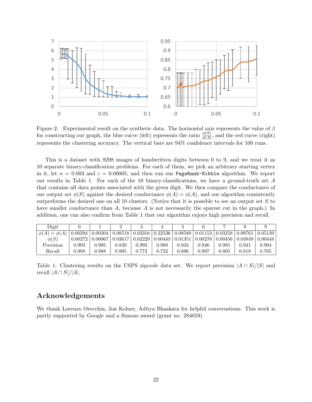
Lo cal Graph Clustering Bey ond Cheeger’s Inequalit y ∗ Zeyuan Allen Zh u zeyuan@csail.mit.edu MIT CSAIL Silvio Lattanzi silviol@google.com Go ogle Researc h V ahab Mirrokni mirrokni@google.com Go ogle Researc h No vem ber 3, 2013 Abstract Motiv ated by applications of large-scale graph clustering, w e study random-walk-based lo c al algorithms whose running times dep end only on the size of the output cluster, rather than the e n tire graph. All previously kno wn such algorithms guaran tee an output conductance of ˜ O ( p φ ( A )) when the target set A has conductance φ ( A ) ∈ [0 , 1]. In this pap er, we improv e it to ˜ O  min n p φ ( A ) , φ ( A ) p Conn ( A ) o  , where the internal connectivit y parameter Conn ( A ) ∈ [0 , 1] is deﬁned as the reciprocal of the mixing time of the random walk ov er the induced subgraph on A . F or instance, using Conn ( A ) = Ω( λ ( A ) / log n ) where λ is the second eigenv alue of the Lapla- cian of the induced subgraph on A , our conductance guarantee can be as go o d as ˜ O ( φ ( A ) / p λ ( A )). This builds an interesting connection to the recen t adv ance of the so-called impr ove d Che e ger’s Ine quality [KLL + 13], whic h says that global sp ectral algorithms can provide a conductance guaran tee of O ( φ opt / √ λ 3 ) instead of O ( p φ opt ). In addition, w e pro vide theoretical guaran tee on the clustering accuracy (in terms of precision and recall) of the output set. W e also pro ve that our analysis is tight, and p erform empirical ev aluation to supp ort our theory on b oth synthetic and real data. It is worth noting that, our analysis outp erforms prior w ork when the cluster is wel l- c onne cte d . In fact, the b etter it is well-connected inside, the more signiﬁcant improv emen t (b oth in terms of conductance and accuracy) we can obtain. Our results shed ligh t on wh y in practice some random-walk-based algorithms p erform better than its previous theory , and help guide future researc h ab out lo cal clustering. 1 In tro duction As a cen tral problem in machine learning, clustering metho ds ha v e b een applied to data mining, computer vision, so cial netw ork analysis. Although a huge num b er of results are kno wn in this area, there is still need to explore metho ds that are robust and eﬃcient on large data sets, and ha ve goo d theoretical guarantees. In particular, several algorithms restrict the num b er of clusters, or imp ose constraints that make these algorithms impractical for large data sets. T o solv e those issues, recen tly , local random-w alk clustering algorithms [ST04, ACL06, ST13, AP09, OT12] ha ve b een in tro duced. The main idea b ehind those algorithms is to ﬁnd a goo d ∗ P art of this w ork was done when the authors were at Google Research NYC. A 9-paged extended abstract con taining the main theorem of this paper has app eared in the pro ceedings of the 30th In ternational Conference on Mac hine Learning (ICML 2013). [ZLM13] 1 cluster around a speciﬁc no de. These tec hniques, thanks to their scalability , has had high impact in practical applications [LLDM09, GLMY11, GS12, A GM12, LLM10, WLS + 12]. Nevertheless, the theoretical understanding of these techniques is still v ery limited. In this pap er, we make an imp ortan t contribution in this direction. First, we relate for the ﬁrst time the p erformance of these lo cal algorithms with the internal c onne ctivity of a cluster instead of analyzing only its external connectivit y . This c hange of p ersp ectiv e is relev an t for practical applications where we are not only in terested to ﬁnd clusters that are lo osely connected with the rest of the world, but also clusters that are w ell-connected in ternally . In particular, we show theoretically and empirically that this in ternal connectivit y is a fundamen tal parameter for those algorithms and, b y leveraging it, it is p ossible to improv e their performances. F ormally , we study the clustering problem where the data set is given b y a similarit y matrix as a graph: giv en an undirected 1 graph G = ( V , E ), w e wan t to ﬁnd a set S that minimizes the relativ e num b er of edges going out of S with resp ect to the size of S (or the size of ¯ S if S is larger than ¯ S ). T o capture this concept rigorously , we consider the (cut) c onductanc e of a set S as: 2 φ ( S ) def = | E ( S, ¯ S ) | min { v ol( S ) , v ol( ¯ S ) } , where vol( S ) def = P v ∈ S deg( v ). Finding S with the smallest φ ( S ) is called the conductance min- imization. This measure is a well-studied measure in diﬀeren t disciplines [SM00, ST04, ACL06, GLMY11, GS12], and has been identiﬁed as one of the most imp ortan t cut-based measures in the lit- erature [Sch07]. Many appro ximation algorithms hav e b een dev elop ed for the problem, but most of them are global ones: their running time dep ends at least linearly on the size of the graph. A recen t trend, initiated by Spielman and T eng [ST04], and then follo wed b y [ST13, A CL06, AP09, OT12], attempts to solve this conductance minimization problem lo c al ly , with running time only dependent on the v olume of the output set. In particular, if there exists a set A ⊂ V with conductance φ ( A ), these local algorithms guar- an tee the existence of some set A g ⊆ A with at least half the volume, suc h that for any “go o d” starting vertex v ∈ A g , they output a set S with conductance φ ( S ) = ˜ O ( p φ ( A )). 1.1 The Internal Connectivit y of a Cluster All lo cal clustering algorithms dev elop ed so far, b oth theoretical ones and empirical ones, only assume that φ ( A ) is small, i.e., A is p o orly connected to ¯ A . Notice that such set A , no matter ho w small φ ( A ) is, may b e p o orly connected or even disconnected inside. This cannot happ en in reality if A is a “go od” cluster, and in practice w e are often interested in ﬁnding mostly go o d clusters. This motiv ates us to study an extra measure on A , that is the connectivity of A , deﬁned as Conn ( A ) def = 1 τ mix ( A ) ∈ [0 , 1] , where τ mix ( A ) is the mixing time for a random walk on the subgraph induced b y A . W e will formalize the deﬁnition of τ mix ( A ) as well as pro vide alternative deﬁnitions to Conn ( A ) in Section 2. It is w orth noting here that one can for instance replace Conn ( A ) with Conn ( A ) def = λ ( A ) log vol( A ) where λ ( A ) is the sp e ctr al gap , i.e., 1 minus the second largest eigen v alue of the random walk matrix on G [ A ]. 1 All our results can b e easily generalized to w eighted graphs. 2 Others also study related notions such as normalize d cut or expansion, e.g., | E ( S, ¯ S ) | min {| S | , | ¯ S |} or | E ( S, ¯ S ) | | S |·| ¯ S | ; there exist w ell-known reductions b et ween the approximation algorithms on them. 2 1.2 Lo cal Clustering for Finding W ell-Connected Clusters In this paper we assume that, in addition to prior w ork, the cluster A is wel l-c onne cte d and satisﬁes the following gap assumption Gap ( A ) def = Conn ( A ) φ ( A ) ≥ Ω (1) , whic h sa ys that A is b etter connected inside than it is connected to ¯ A . This assumption makes sense in real world scenarios for tw o main reasons. First, in practice w e are often interested in retrieving clusters that ha ve a b etter connectivity within themselv es than with the rest of the graph. Second, in sev eral applications the edges of the graph represen t pairwise similarit y scores extracted from a mac hine learning algorithm and so w e w ould exp ect similar nodes to b e w ell connected within themselv es while diss imilar no des to b e lo osely connected. As a result, it is not surprising that the notion of connectivit y is not new. F or instance [KVV04] studied a bicriteria optimization for this ob jectiv e. How ever, lo cal algorithms based on the ab ov e gap assumption is not well studied. 3 Our P ositive Result. Under the gap assumption Gap ( A ) ≥ Ω(1), can we guarantee any b etter conductance than the previously shown ˜ O ( p φ ( A )) ones? W e prov e that the answ er is aﬃrmative, along with theoretical guaran tees on the accuracy of the output cluster. In particular, w e pro ve: Theorem 1. Ther e exists a c onstant c > 0 such that, for any non-empty set A ⊂ V with Gap ( A ) ≥ c , ther e exists some A g ⊆ A with vol( A g ) ≥ 1 2 v ol( A ) such that, when cho osing a starting vertex v ∈ A g , the PageRank - Nibble algorithm outputs a set S with 1. v ol( S \ A ) ≤ O  φ ( A ) Conn ( A )  · vol( A ) = O  1 Gap ( A )  · vol( A ) , 2. v ol( A \ S ) ≤ O  φ ( A ) Conn ( A )  · vol( A ) = O  1 Gap ( A )  · vol( A ) , 3. φ ( S ) ≤ O  φ ( A ) √ Conn ( A )  = O  √ φ ( A ) √ Gap ( A )  , and with running time O  vol( A ) Conn ( A )  ≤ O  vol( A ) φ ( A )  . W e interpret the ab o v e theorem as follows. The ﬁrst tw o prop erties imply that under Gap ( A ) ≥ Ω(1), the volume for vol( S \ A ) and vol( A \ S ) are b oth small in comparison to vol( A ), and the larger the gap is, the more accurate S appro ximates A . 4 F or the third prop ert y on the conductance φ ( S ), we notice that our guaran tee O ( p φ ( A ) / Gap ( A )) ≤ O ( p φ ( A )) outp erforms all previous w ork on lo cal clustering under this parameter regime. In addition, Gap ( A ) might be very large in reality . F or instance when A is a v ery-well-connected cluster it migh t satisfy Conn ( A ) = p olylog ( n ). In this case our Theorem 1 guarantees a p olylog ( n ) true-appro ximation to the conductance. Our pro of of Theorem 1 uses almost the same PageRank algorithm as [ACL06], but with a v ery diﬀerent analysis sp eciﬁcally designed for our gap assumption. 5 This algorithm is simple and clean, and can b e describ ed in four steps: 1) compute the (appro ximate) PageRank v ector starting from a vertex v ∈ A g with carefully chosen parameters, 2) sort all the v ertices according to their (normalized) probabilities in this v ector, 3) study all swe ep cuts that are those separating 3 One relev ant paper using this assumption is [MMV12], who pro vided a glob al SDP-based algorithm to approximate the conductance. 4 V ery recently , [WLS + 12] studied a v ariant of the P ageRank random walk and their ﬁrst exp erimen t —although analyzed in a diﬀerent p erspective— essentially conﬁrmed our ﬁrst tw o prop erties in Theorem 1. How ever, they hav e not attempted to explain this in theory . 5 In terestingly , their theorems do not imply any new result in our setting at least in any obvious wa y , and thus pro ofs diﬀeren t from the previous work are necessary in this paper. T o the best of our knowledge, equation (3.1) is the only part that is a consequence of their result, and w e will men tion it without proof. 3 high-v alue v ertices from low-v alue ones, and 4) output the sweep cut with the best conductance. See Algorithm 1 on page 18 for details. An Unconditional Result. In realit y one ma y ﬁnd it hard to c heck if the assumption Gap ( A ) ≥ Ω(1) is satisﬁed, and thus we state a simple corollary to the ab o v e theorem without this assumption. Note that some Corollary 2. F or any non-empty set A ⊂ V , ther e exists some A g ⊆ A with vol( A g ) ≥ 1 2 v ol( A ) such that, when cho osing a starting vertex v ∈ A g , the PageRank - Nibble algorithm runs in time O  vol( A ) φ ( A )  and outputs a set S with φ ( S ) ≤ ( O  p φ ( A ) · log v ol( A )  , if Conn ( A ) < c · φ ( A ) ; O  φ ( A ) / p Conn ( A )  , if Conn ( A ) ≥ c · φ ( A ) . Or mor e brieﬂy: φ ( S ) ≤ ˜ O  min n p φ ( A ) , φ ( A ) p Conn ( A ) o  . R e c al l that one c an cho ose Conn ( A ) = 1 /τ mix ( A ) or Conn ( A ) = λ ( A ) / log vol( A ) . The proof to the ab o v e corollary is straigh tforward. One can simply study t wo diﬀerent analyses of the same algorithm PageRank-Nibble (with slightly diﬀeren t parameters): one is ours, whic h only works when Gap ( A ) ≥ c ; and the other one is the original analysis of Andersen, Ch ung and Lang [A CL06], whic h guaran tees an output conductance of O ( p φ ( A ) log vol( A )) in the same running time. Connection to the Impro ved Cheeger’s Inequality . Almost sim ultaneous to the app earance of the ﬁrst v ersion of this pap er [ZLM13], Kw ok et al. [KLL + 13] disco ver indep endently a similar b eha vior to our result but on global and sp ectral algorithms, whic h they call the impr ove d Che e ger’s Ine quality . Let φ opt b e the optimal conductance of G , and v the second eigen vector of the normalized Laplacian matrix of G . Using Cheeger’s Inequalit y , one can sho w that the b est sweep cut on v pro vides a conductance of O ( p φ opt ); the improv ed Cheeger’s Inequalit y sa ys that the conductance guaran tee can be impro ved to O  φ opt √ λ 3  where λ 3 is the third smallest eigenv alue. In other words, the performance (for the same algorithm) is improv ed when for instance b oth sides of the desired cut are well-connected (e.g., expanders). Our Theorem 1 and Corollary 2 show that this same b eha vior o ccurs for random-w alk based local algorithms. 1.3 Tigh tness of Our Analysis W e also pro ve that our analysis is tight. Theorem 3. F or any c onstant c > 0 , ther e exists a family of gr aphs G = ( V , E ) and a non-empty A ⊂ V with Gap ( A ) > c , such that for al l starting vertic es v ∈ A , none of the swe ep-cut b ase d algo- rithm on the PageR ank ve ctor c an output a set S with c onductanc e b etter than O ( φ ( A ) / p Conn ( A )) . W e prov e this tightness result by illustrating a hard instance, and proving upp er and low er b ounds on the probabilities of reaching sp eciﬁc vertices (up to a very high precision). In fact, ev en the description of the hard instance is somewhat non-trivial and diﬀeren t from the impro ved Cheeger’s Inequality case where the hard instance simply a cycle. Although Theorem 3 do es not fully rule out the existence of another local algorithm that can p erform better than O ( φ ( A ) / p Conn ( A )), we conjecture that all existing random-walk-based lo cal 4 clustering algorithms share this same hard instance and cannot outp erform O ( φ ( A ) / p Conn ( A )). This is analogous to the classical case (without the connectivit y assumption) where all existing lo cal algorithms provide ˜ O ( p φ ( A )) due to Cheeger’s inequality . In the ﬁrst v ersion of this pap er [ZLM13], we raised as an interesting op en question to design a ﬂo w-based local algorithm to o v ercome this barrier under our connectivity assumption Gap ( A ) ≥ Ω(1). Lately , Orecc hia and Zh u ha ve made this p ossible and obtained an O (1)-approximation to conductance under this same assumption [OZ14]. Their result is built on ours: it requires a preliminary run of the PageRank-Nibble algorithm, the use of our b etter analysis, and a non-trivial lo calization of the cut-impr ovement algorithm from the seminar w ork of Andersen and Lang [AL08]. It is w orth pointing out that they ac hieve this b etter conductance appro ximation at the exp ense of losing the accuracy guaran tee of the output cluster (see the ﬁrst tw o items of our Theorem 1). 1.4 Prior W ork Most relev ant to our work are the ones on lo cal algorithms for clustering. After the ﬁrst such result [ST04, ST13], Andersen, Chung and Lang [A CL06] simply compute a Pagerank random w alk v ector and then show that one of its sweep cuts satisﬁes conductance O ( p φ ( A ) log vol( A )). The computation of this Pagerank v ector is deterministic and is essen tially the algorithm we adopt in this pap er. [AP09, OT12] use the theory of ev olving set from [MP03]. They study a sto c hastic v olume-biased ev olving set process that is similar to a random work. This leads to a b etter (but probabilistic) running time and but essen tially with the same conductance guaran tee. The problem of conductance minimization is UGC-hard to appro ximate within any constan t factor [CKK + 06]. On the p ositiv e side, sp ectral partitioning algorithms output a solution with conductance O ( p φ opt ) where this idea traces back to [Alo86] and [SJ89]; Leigh ton and Rao [LR99] pro vide a ﬁrst O (log n ) approximation; and Arora, Rao and V azirani [AR V09] pro vide a O ( √ log n ) appro ximation. Those results, along with recen t improv emen ts on the running time by for instance [OSV12, OSVV08, AHK10, AK07, She09], are all glob al algorithms: their time complexities dep end at least linearly on the size of G . There are also w ork in machine learning to make suc h global algorithms practical, including the work of [LC10] for sp ectral partitioning. Less relev an t to our work are sup ervised learning on ﬁnding clusters, and there exist algorithms that hav e a sub-linear running time in terms of the size of the training set [ZCZ + 09, SS08]. On the empirical side, random-w alk-based graph clustering algorithms ha ve been widely used in practice [GS12, GLMY11, ACE + 13, A GM12] as they can b e implemented in a distributed manner for v ery big graphs using map-reduce or similar distributed graph mining algorithms [LLDM09, GLMY11, GS12, AGM12]. Suc h lo cal algorithms hav e been applied for (ov erlapping) clustering of big graphs for distributed computation [A GM12], or communit y detection on huge Y outub e video graphs [GLMY11]. There also exist v arian ts of the random walk, such as the multi-agen t random w alk, that are known to b e lo cal and perform w ell in practice [AvL10]. More recently , [WLS + 12] studied a slight v arian t of the P ageRank random walk and p erformed supp ortiv e experiments on it. Their exp eriments conﬁrmed the ﬁrst tw o properties in our Theo- rem 1, but their theoretical results are not strong enough to conﬁrm it. This is b ecause there is no w ell-connectedness assumption in their pap er so they are forced to study random w alks that start from a random v ertex selected in A , rather than a ﬁxed one lik e ours. In addition, they hav e not argued ab out the conductance (lik e our third prop ert y in Theorem 1) of the set they output. Clustering is an imp ortan t tec hnique for communit y detections, and indeed lo cal clustering algorithms ha ve b een widely applied there, see for instance [AL06]. Sometimes researchers care ab out ﬁnding all comm unities, i.e., clusters, in the en tire graph and this can be done by rep eatedly applying lo cal clustering algorithms. Ho wev er, if the ultimate goal is to ﬁnd all clusters, global 5 algorithms p erform b etter in at least in terms of minimizing conductance [LLDM09, GLMY11, GS12, AGM12, LLM10]. 1.5 Roadmap W e provide necessary preliminaries in Section 2, and they are follo wed b y the high level ideas for the pro ofs (as long as the actual proofs) for Theorem 1 in Section 3 and Section 4. W e then brieﬂy describ e how to pro ve our tightness result in Section 5 while deferring the analysis to App endix A, and end this pap er with empirical studies in Section 6. In App endix B we brieﬂy summarize and show some prop ert y for the algorithm Approximate-PR of Andersen, Chung and Lang for completeness. 2 Preliminaries 2.1 Problem F orm ulation Consider an undirected graph G ( V , E ) with n = | V | v ertices and m = | E | edges. F or an y v ertex u ∈ V the degree of u is denoted b y deg ( u ), and for an y subset of the v ertices S ⊆ V , volume of S is denoted by vol( S ) def = P u ∈ S deg( u ). Giv en tw o subsets A, B ⊂ V , let E ( A, B ) b e the set of edges b et w een A and B . F or a vertex set S ⊆ V , we denote b y G [ S ] the induced subgraph of G on S with outgoing edges remo ved, b y deg S ( u ) the degree of vertex u ∈ S in G [ S ], and by v ol S ( T ) the volume of T ⊆ S in G [ S ]. W e resp ectiv ely deﬁne the (cut) c onductanc e and the set c onductanc e of a non-empt y set S ⊆ V as follows: φ ( S ) def = | E ( S, ¯ S ) | min { v ol( S ) , v ol( ¯ S ) } , φ s ( S ) def = min ∅⊂ T ⊂ S | E ( T , S \ T ) | min { v ol S ( T ) , vol S ( S \ T ) } . Here φ s ( S ) is classically known as the conductance of S on the induced subgraph G [ S ]. W e formalize our goal in this pap er as a pr omise pr oblem . Sp eciﬁcally , we assume the existence of a non-empty target cluster of the v ertices A ⊂ V satisfying v ol( A ) ≤ 1 2 v ol( V ). This set A is not kno wn to the algorithm. The goal is to ﬁnd some set S that “reasonably” approximates A , and at the same time b e lo c al : running in time proportional to v ol( A ) rather than n or m . Our assumption. W e assume that the target set A is wel l-c onne cte d , i.e., the follo wing gap assumption: Gap ( A ) def = Conn ( A ) φ ( A ) def = 1 /τ mix ( A ) φ ( A ) ≥ Ω(1) (Gap Assumption) holds throughout this pap er. This assumption can be understo od as the cluster A is more w ell- connected inside than it is connected to ¯ A . F or all the p ositiv e results of this paper, one can replace this assumption with Gap ( A ) = Conn ( A ) φ ( A ) def = λ ( A ) / log vol( A ) φ ( A ) ≥ Ω(1) , or (Gap Assumption’) Gap ( A ) = Conn ( A ) φ ( A ) def = φ 2 s ( A ) / log vol( A ) φ ( A ) ≥ Ω(1) (Gap Assumption”) 6 • Here λ ( A ) is the sp e ctr al gap , that is the diﬀerence b et w een the ﬁrst and second largest eigen v alues of the lazy random w alk matrix on G [ A ]. (Notice that the largest eigenv alue of any random w alk matrix is alwa ys 1.) Equiv alently , λ ( A ) can b e deﬁned as the second smallest eigenv alue of the Laplacian matrix of G [ A ]. • Here τ mix is the mixing time for the r elative p ointwise distanc e in G [ A ] (cf. Deﬁnition 6.14 in [MR95]), that is, the minimum time required for a lazy random w alk to mix r elatively on all v ertices regardless of the starting distribution. F ormally , let W A b e the lazy random w alk matrix on G [ A ], and π b e the stationary distribution on G [ A ] that is π ( u ) = deg A ( u ) / v ol A ( A ), then τ mix = min  t ∈ Z ≥ 0 : max u,v     ( χ v W t A )( u ) − π ( u ) π ( u )     ≤ 1 2  . Notice that using Cheeger’s inequality , w e alwa ys hav e φ s ( A ) 2 log vol( A ) ≤ O  λ ( A ) log vol( A )  ≤ O  1 τ mix  . This is why (Gap Assumption) is weak er than (Gap Assumption’) whic h is then weak er than (Gap Assumption”). Input parameters. Similar to prior w ork on lo cal clustering, w e assume the algorithm tak es as input: • Some “go o d” starting vertex v ∈ A , and an or acle to output the set of neighb ors for any given vertex. This requiremen t is essen tial b ecause without such an oracle the algorithm ma y hav e to read all inputs and cannot b e sublinear in time; and without a starting vertex the sublinear-time algorithm may b e unable to ev en ﬁnd an elemen t in A . W e also need v to b e “go od”, as for instance the vertices on the b oundary of A ma y not b e helpful enough in ﬁnding go o d clusters. W e call the set of goo d v ertices A g ⊆ A , and a lo cal algorithm needs to ensure that A g is large, e.g., vol( A g ) ≥ 1 2 v ol( A ). This assumption is una voidable in all lo cal clustering w ork. One can replace this 1 2 b y any other constant at the exp ense of worsening the guarantees b y a constan t factor. • The value of Conn ( A ) . In practice Conn ( A ) can b e viewed as a parameter and can be tuned for sp eciﬁc data. This is in con trast to the v alue of φ ( A ) that is the target conductance and do es not need to b e kno wn by the algorithm. In prior work when φ ( A ) is the only quantit y studied, φ ( A ) plays b oth roles as a (kno wn) tuning parameter and as a target. • A value v ol 0 satisfying v ol( A ) ∈ [v ol 0 , 2v ol 0 ] . This requiremen t is optional since otherwise the algorithm can try out diﬀerent p o wers of 2 and pic k the smallest one with a v alid output. It blows up the running time only by a constan t factor for lo cal algorithms, since the running time of the last trial dominates. 2.2 P ageRank Random W alk W e use the conv ention of writing v ectors as ro w vectors in this pap er. Let A b e the adjacency matrix of G , and let D b e the diagonal matrix with D ii = deg( i ), then the lazy r andom walk matrix W def = 1 2 ( I + D − 1 A ). Accordingly , the P ageRank v ector pr s,α , is deﬁned to b e the unique solution of the follo wing linear equation (cf. [A CL06]): pr s,α = αs + (1 − α ) pr s,α W , 7 where α ∈ (0 , 1] is the telep ort pr ob ability and s is a starting ve ctor . Here s is usually a probability v ector: its entries are in [0 , 1] and sum up to 1. F or technical reasons we ma y use an arbitrary (and p ossibly negativ e) v ector s inside the proof. When it is clear from the con text, w e drop α in the subscript for cleanness. Giv en a vertex u ∈ V , let χ u ∈ { 0 , 1 } | V | b e the indicator vector that is 1 only at vertex u . Giv en non-empty subset S ⊆ V w e denote b y π S the degree-normalized uniform distribution on S , that is, π S ( u ) = deg( u ) vol( S ) when u ∈ S and 0 otherwise. V ery often we study a PageRank v ector when s = χ v is an indicator v ector, and if so w e abbreviate pr χ v b y pr v . One equiv alen t w ay to study pr s is to imagine the follo wing random pro cedure: ﬁrst pick a non-negativ e integer t ∈ Z ≥ 0 with probabilit y α (1 − α ) t , then p erform a lazy random walk starting at vector s with exactly t steps, and at last deﬁne pr s to b e the vector describing the probabilit y of reaching each v ertex in this random pro cedure. In its mathematical form ula we hav e (cf. [Hav02, ACL06]): Prop osition 2.1. pr s = αs + α P ∞ t =1 (1 − α ) t ( sW t ) . This implies that pr s is linear: a · pr s + b · pr t = pr as + bt . 2.3 Appro ximate PageRank V ector In the seminal work of [ACL06], they deﬁned approximate P ageRank vectors and designed an algorithm to compute them eﬃciently . Deﬁnition 2.2. A n ε -approximate P ageRank vector p for pr s is a nonne gative PageR ank ve ctor p = pr s − r wher e the ve ctor r is nonne gative and satisﬁes r ( u ) ≤ ε deg ( u ) for al l u ∈ V . Prop osition 2.3. F or any starting ve ctor s with k s k 1 ≤ 1 and ε ∈ (0 , 1] , one c an c ompute an ε -appr oximate PageR ank ve ctor p = pr s − r for some r in time O  1 εα  , with v ol(supp( p )) ≤ 2 (1 − α ) ε . F or completeness we pro vide the algorithm and its pro of in App endix B. It can b e veriﬁed that: ∀ u ∈ V , pr s ( u ) ≥ p ( u ) ≥ pr s ( u ) − ε deg ( u ) . (2.1) 2.4 Sw eep Cuts Giv en any appro ximate PageRank v ector p , the swe ep cut (or thr eshold cut) technique is the one to sort all vertices according to their degree-normalized probabilities p ( u ) deg( u ) , and then study only those cuts that separate high-v alue vertices from low-v alue vertices. More sp eciﬁcally , let v 1 , v 2 , . . . , v n b e the decreasing order o ver all vertices with resp ect to p ( u ) deg( u ) . Then, deﬁne swe ep sets S p j def = { v 1 , . . . , v j } for eac h j ∈ [ n ], and sw eep cuts are the corresp onding cuts ( S p j , S p j ). Usually giv en a v ector p , one lo oks for the b est cut: min j ∈ [ n − 1] φ ( S p j ) . In almost all the cases, one only needs to enumerate j ov er p ( v j ) > 0, so the ab o ve sw eep cut pro cedure runs in time O  v ol(supp( p )) + | supp( p ) | · log | supp( p ) |  . This running time is dominated b y the time to compute p (see Proposition 2.3), so it is negligible. 8 2.5 Lo v´ asz-Simono vits Curve Our proof requires the technique of L ov´ asz-Simonovits Curve that has been more or less used in all lo cal clustering algorithms so far. This technique was originally introduced b y Lov´ asz and Simono vits [LS90, LS93] to study the mixing rate of Marko v chains. In our language, from a probabilit y v ector p on vertices, one can introduce a function p [ x ] on real n umber x ∈ [0 , 2 m ]. This function p [ x ] is piecewise linear, and is characterized b y all of its end p oin ts as follows (letting p ( S ) def = P a ∈ S p ( a )): p [0] def = 0 , p [v ol( S p j )] def = p ( S p j ) for eac h j ∈ [ n ] . In other w ords, for an y x ∈ [v ol( S p j ) , v ol( S p j +1 )], p [ x ] def = p ( S p j ) + x − vol( S p j ) deg( v j +1 ) p ( v j +1 ) . Note that p [ x ] is increasing and conca ve. 3 Our Accuracy Guaran tee In this section, we study P ageRank random w alks that start at a vertex v ∈ A with telep ort probabilit y α . W e claim the range of in teresting α is  Ω( φ ( A )) , O ( Conn ( A ))  . This is because, at a high level, when α  φ ( A ) the random w alk will leak too muc h to ¯ A ; while when α  Conn ( A ) the random w alk will not mix well inside A . In prior w ork, α is chosen to b e Θ( φ ( A )), and w e will adopt the c hoice of α = Θ( Conn ( A )) = Θ( φ ( A ) · Gap ( A )). Intuitiv ely , this c hoice of α ensures that under the condition the random walk mixes inside, it makes the walk leak as little as p ossible to ¯ A . W e prov e the ab ov e intuition rigorously in this section. Speciﬁcally , we ﬁrst show some prop erties on the exact PageRank v ector in Section 3.1, and then mo ve to the appro ximate v ector in Section 3.2. This essentially prov es the ﬁrst tw o prop erties of Theorem 1. 3.1 Prop erties on the Exact V ector W e ﬁrst in tro duce a new notation e pr s , that is the P ageRank vector (with telep ort probability α ) starting at v ector s but w alking on the subgraph G [ A ]. Next, we c ho ose the set of “go o d” starting v ertices A g to satisfy tw o prop erties: (1) the total probabilit y of leak age is uppe r b ounded by 2 φ ( A ) α , and (2) pr v is close to e pr v for vertices in A . Note that the latter implies that pr v mixes well inside A as long as e pr v do es so. Lemma 3.1. Ther e exists a set A g ⊆ A with volume vol( A g ) ≥ 1 2 v ol( A ) such that, for any vertex v ∈ A g , in a PageR ank ve ctor with telep ort pr ob ability α starting at v , we have: X u 6∈ A pr v ( u ) ≤ 2 φ ( A ) α . (3.1) In addition, ther e exists a non-ne gative leak age v ector l ∈ [0 , 1] | V | with norm k l k 1 ≤ 2 φ ( A ) α satisfying ∀ u ∈ A, pr v ( u ) ≥ e pr v ( u ) − e pr l ( u ) . (3.2) (Details of the pro of are in Section 3.3.) 9 Pr o of sketch. The proof for the ﬁrst property (3.1) is classical and can b e found in [ACL06]. The idea is to study an auxiliary PageRank random w alk with telep ort probability α starting at the degree-normalized uniform distribution π A , and by simple computation, this random w alk leaks to ¯ A with probabilit y no more than φ ( A ) /α . Then, using Mark ov b ound, there exists A g ⊆ A with v ol( A g ) ≥ 1 2 v ol( A ) suc h that for each starting v ertex v ∈ A g , this leak age is no more than 2 φ ( A ) α . This implies (3.1) immediately . The interesting part is (3.2). Note that pr v can b e view ed as the probabilit y vector from the follo wing random procedure: start from vertex v , then at eac h step with probability α let the walk stop, and with probabilit y (1 − α ) follow the matrix W to go to one of its neighbors (or itself ) and contin ue. Now, w e divide this pro cedure into t wo rounds. In the ﬁrst round, w e run the same P ageRank random walk but whenev er the walk wan ts to use an outgoing edge from A to leak, w e let it stop and temp orarily “hold” this probabilit y mass. W e deﬁne l to b e the non-negativ e v ector where l ( u ) denotes the amount of probability that w e hav e “held” at vertex u . In the second round, we contin ue our random w alk only from vector l . It is worth noting that l is non-zero only at b oundary vertices in A . Similarly , we divide the P ageRank random walk for e pr v in to t w o rounds. In the ﬁrst round w e hold exactly the same amount of probabilit y l ( u ) at b oundary vertices u , and in the second round w e start from l but contin ue this random walk only within G [ A ]. T o bound the diﬀerence b etw een pr v and e pr v , we note that they share the same pro cedure in the ﬁrst round; while for the second round, the random procedure for pr v starts at l and walks tow ards V \ A (so in the worst case it may nev er come bac k to A again), while that for e pr v starts at l and w alks only inside G [ A ] so induces a probabilit y vector e pr l on A . This gives (3.2). A t last, to see k l k 1 ≤ 2 φ ( A ) α , one just needs to v erify that l ( u ) is essentially the probability that the original P ageRank random walk leaks from v ertex u . Then, k l k 1 ≤ 2 φ ( A ) α follo ws from the fact that the total amoun t of leak age is upp er b ounded b y 2 φ ( A ) α . As men tioned earlier, we w an t to use (3.2) to low er b ound pr v ( u ) for v ertices u ∈ A . W e ac hieve this b y ﬁrst lo wer b ounding e pr v whic h is the P ageRank random w alk on G [ A ]. Given a telep ort probabilit y α that is small compared to Conn ( A ), this random walk should mix w ell. W e formally state it as the following lemma, and pro vide its proof in the Section 3.4. Lemma 3.2. When α ≤ O ( Conn ( A )) we have that ∀ u ∈ A, e pr v ( u ) ≥ 4 5 deg A ( u ) v ol( A ) . Her e deg A ( u ) is the de gr e e of u on G [ A ] , but vol( A ) is with r esp e ct to the original gr aph. 3.2 Prop erties of the Appro ximate V ector F rom this section on we alw a ys use α ≤ O ( Conn ( A )). W e then ﬁx a starting v ertex v ∈ A g and study an ε -appro ximate Pagerank v ector for pr v . W e choose ε = 1 10 · vol 0 ∈ h 1 20v ol( A ) , 1 10v ol( A ) i . (3.3) F or notational simplicity , we denote by p this ε -approximation and recall from Section 2.3 that p = pr χ v − r where r is a non-negative vector with 0 ≤ r ( u ) ≤ ε deg ( u ) for every u ∈ V . Recall from (2.1) that pr v ( u ) ≥ p ( u ) ≥ pr v ( u ) −  · deg( u ) for all u ∈ V . W e no w rewrite Lemma 3.1 in the language of approximate P ageRank vectors using Lemma 3.2: 10 Corollary 3.3. F or any v ∈ A g and α ≤ O ( Conn ( A )) , in an ε -appr oximate PageR ank ve ctor to pr v denote d by p = pr χ v − r , we have: X u 6∈ A p ( u ) ≤ 2 φ ( A ) α and X u 6∈ A r ( u ) ≤ 2 φ ( A ) α . In addition, ther e exists a non-ne gative leak age vector l ∈ [0 , 1] V with norm k l k 1 ≤ 2 φ ( A ) α satisfying ∀ u ∈ A, p ( u ) ≥ 4 5 deg A ( u ) v ol( A ) − deg( u ) 10v ol( A ) − e pr l ( u ) . Pr o of. The only inequality that requires a proof is P u 6∈ A r ( u ) ≤ 2 φ ( A ) α . In fact, if one tak es a closer lo ok at the algorithm to compute an appro ximate Pagerank vector (cf. App endix B), the total probabilit y mass that will b e sen t to r on v ertices outside A , is upper b ounded by the probability of leak age. How ev er, the latter is upp er bounded b y 2 φ ( A ) α when we c ho ose A g . W e are now ready to state the main lemma of this section. W e sho w that for all reasonable sw eep sets S on this probability v ector p , it satisﬁes that vol( S \ A ) and vol( A \ S ) are b oth at most O  φ ( A ) α v ol( A )  . Lemma 3.4. In the same deﬁnition of α and p fr om Cor ol lary 3.3, let swe ep set S c def =  u ∈ V : p ( u ) ≥ c deg( u ) vol( A )  for any c onstant c < 3 5 , then we have the fol lowing guar ante es on the size of S c \ A and A \ S c : 1. v ol( S c \ A ) ≤ 2 φ ( A ) αc v ol( A ) , and 2. v ol( A \ S c ) ≤  2 φ ( A ) α ( 3 5 − c ) + 8 φ ( A )  v ol( A ) . Pr o of. First w e notice that p ( S c \ A ) ≤ p ( V \ A ) ≤ 2 φ ( A ) α o wing to Corollary 3.3, and for each v ertex u ∈ S c \ A it must satisfy p ( u ) ≥ c deg( u ) vol( A ) . Those combined imply vol( S c \ A ) ≤ 2 φ ( A ) αc v ol( A ) proving the ﬁrst property . W e show the second property in tw o steps. First, let A b b e the set of v ertices in A such that 4 5 deg A ( u ) vol( A ) − deg( u ) 10vol( A ) < 3 5 deg( u ) vol( A ) . Any such vertex u ∈ A b m ust hav e deg A ( u ) < 7 8 deg( u ). This implies that u has to b e on the b oundary of A and vol( A b ) ≤ 8 φ ( A )v ol( A ). Next, for a vertex u ∈ A \ A b w e ha ve (using Corollary 3.3 again) p ( u ) ≥ 3 5 deg( u ) vol( A ) − e pr l ( u ). If w e further assume u 6∈ S c w e ha v e p ( u ) < c deg( u ) vol( A ) , that implies e pr l ( u ) ≥ ( 3 5 − c ) deg( u ) vol( A ) . As a consequence, the total v olume for suc h vertices (i.e., v ol( A \ ( A b ∪ S c ))) cannot exceed k e pr l k 1 3 / 5 − c v ol( A ). At last, we notice that e pr l is a non-negative probability vector coming from a random w alk pro cedure, so k e pr l k 1 = k l k 1 ≤ 2 φ ( A ) α . This in sum provides that v ol( A \ S c ) ≤ v ol( A \ ( A b ∪ S c )) + vol( A b ) ≤ 2 φ ( A ) α ( 3 5 − c ) + 8 φ ( A ) ! v ol( A ) . Note that if one c ho oses α = Θ( Conn ( A )) in the ab o v e lemma, b oth those t wo volumes are at most O (v ol( A ) / Gap ( A )) satisfying the ﬁrst t w o properties of Theorem 1. 11 3.3 Pro of of Lemma 3.1 Lemma 3.1. Ther e exists a set A g ⊆ A with volume vol( A g ) ≥ 1 2 v ol( A ) such that, for any vertex v ∈ A g , in a PageR ank ve ctor with telep ort pr ob ability α starting at v , we have: X u 6∈ A pr v ( u ) ≤ 2 φ ( A ) α . (3.1) In addition, ther e exists a non-ne gative leak age vector l ∈ [0 , 1] V with norm k l k 1 ≤ 2 φ ( A ) α satisfying ∀ u ∈ A, pr v ( u ) ≥ e pr v ( u ) − e pr l ( u ) . (3.2) Leak age even t. W e b egin our pro of b y deﬁning the le aking event in a random w alk pro cedure. W e start the deﬁnition of a lazy random walk and then mov e to a PageRank random walk. At high lev el, w e sa y that a lazy random w alk of length t starting at a vertex u ∈ A do es not le ak from A if it nev er go es out of A , and let Leak ( u, t ) denote the probability that such a random walk leaks. More formally , for eac h v ertex u ∈ V in the graph with degree deg( u ), recall that in its random w alk graph it actually has degree 2 deg( u ), with deg ( u ) edges going to each of its neigh b ors, and deg( u ) self-lo ops. F or a vertex u ∈ A , let us call its neighboring edge ( u, v ) ∈ E a b ad e dge if v 6∈ A . In addition, if u has k bad edges, we also distinguish k self-lo ops at u in the lazy random walk graph, and call them b ad self-lo ops . Now, w e sa y that a random walk do es not leak from A , if it never uses any of those b ad e dges of self-lo ops . The purp ose of this deﬁnition is to mak e sure that if a random w alk chooses only go o d edges at each step, it is equiv alent to a lazy random walk on the induced subgraph G [ A ] with outgoing edges remov ed. F or a P ageRank random walk with telep ort probability α starting at a v ertex u , recall that it is also a random pro cedure and can b e viewed as ﬁrst picking a length t ∈ { 0 , 1 , . . . } with probabilit y α (1 − α ) t , and then p erforming a lazy random w alk of length t starting from u . By the linearit y of random w alk v ectors, the probabilit y of leak age for this P agerank random walk is exactly P ∞ t =0 α (1 − α ) t Leak ( u, t ). Upp er b ounding leak age. W e now giv e an upp er b ound on the probability of leak age. W e start with an auxiliary lazy random walk of length t starting from a “uniform” distribution π A ( u ). Recall that π A ( u ) = deg( u ) vol( A ) for u ∈ A and 0 else where. W e now wan t to show that this random w alk leaks with probabilit y at most 1 − tφ ( A ). 6 This is because, one can verify that: (1) in the ﬁrst step of this random w alk, the probabilit y of leak age is upp er b ounded b y φ ( A ) b y the deﬁnition of conductance; and (2) in the i -th step in general, this random walk satisﬁes ( π A W i − 1 )( u ) ≤ π A ( u ) for an y vertex u ∈ A , and therefore the probability of leak age in the i -th step is upp er b ounded b y that in the ﬁrst step. In sum, the total leak age is at most tφ ( A ), or equiv alen tly , P u ∈ A π A ( u ) Leak ( u, t ) ≤ tφ ( A ). W e now sum this up ov er the distribution of t in a P ageRank random w alk: X u ∈ A π A ( u ) ∞ X t =0 α (1 − α ) t Leak ( u, t ) ! = ∞ X t =0 α (1 − α ) t X u ∈ A π A ( u ) Leak ( u, t ) ! ≤ ∞ X t =0 α (1 − α ) t tφ ( A ) = φ ( A )(1 − α ) α . 6 Note that this step of the pro of coincides with that of Prop osition 2.5 from [ST13]. Our tφ ( A ) is oﬀ b y a factor of 2 from theirs b ecause we also regard bad self-lo ops as edges that leak. 12 This implies, using Marko v b ound, there exists a set A g ⊆ A with volume v ol( A g ) ≥ 1 2 v ol( A ) satisfying ∀ v ∈ A g , ∞ X t =0 α (1 − α ) t Leak ( v , t ) ≤ 2 φ ( A )(1 − α ) α < 2 φ ( A ) α , (3.4) or in w ords: the probabilit y of leak age is at most 2 φ ( A )(1 − α ) α in a P agerank random walk that starts at vertex v ∈ A g . This inequality immediately implies (3.1), so for the rest of the pro of, w e concen trate on (3.2). Lo w er b ounding pr . No w we pick some v ∈ A g , and try to lo wer b ound pr v . T o b egin with, we deﬁne t w o | A | × | A | lazy random walk matrices on the induced subgraph G [ A ] (recall that deg ( u ) is the degree of a vertex and for u ∈ A we denote b y deg A ( u ) the num b er of neighbors of u inside A ): 1. Matrix c W . This is a random w alk matrix assuming that all outgoing edges from A b eing “phan tom”, that is, at eac h vertex u ∈ A : • it picks eac h neighbor in A with probabilit y 1 2 deg ( u ) , and • it stays where it is with probability deg A ( u ) 2 deg ( u ) . F or instance, let u b e a v ertex in A with four neighbors w 1 , w 2 , w 3 , w 4 suc h that w 1 , w 2 , w 3 ∈ A but w 4 6∈ A . Then, for a lazy random w alk using matrix c W , if it starts from u then in the next step it stays at u with probability 3 / 8, and go es to w 1 , w 2 and w 3 eac h with probability 1 / 8. Note that, for the rest 1 / 4 probabilit y (whic h corresp onds to w 4 ) it go es nowher e and this random w alk “disapp ears”! This can b e viewed as that the random walk leaks A . 2. Matrix f W . This is a random w alk matrix assuming that all outgoing edges from A are remo ved, that is, at eac h v ertex u ∈ A : • it picks eac h neighbor in A with probabilit y 1 2 deg A ( u ) , and • it stays where it is with probability 1 2 . The ma jor diﬀerence betw een f W and c W is that they are normalized b y diﬀerent degrees in the ro ws, and the rows of f W sum up to 1 but those of c W do not necessarily . More speciﬁcally , if we denote b y D the diagonal matrix with deg( u ) on the diagonal for eac h v ertex u ∈ A , and D A the diagonal matrix with deg A ( u ) on the diagonal, then c W = D − 1 D A f W . It is worth noting that, if one sums up all entries of the nonnegative vector χ v c W t , the summation is exactly 1 − Leak ( v , t ) b y our deﬁnition of Leak . W e now precisely study the diﬀerence b etw een f W and c W using the following claim. Claim 3.5. Ther e exists non-ne gative ve ctors l t for al l t ∈ { 1 , 2 , . . . } satisfying: k l t k 1 = Leak ( v , t ) − Leak ( v , t − 1) , and χ v c W t =  χ v c W t − 1 − l t  f W . 13 Pr o of. T o obtain the result of this claim, w e write χ v c W t =  χ v c W t − 1  D − 1 D A f W =  χ v c W t − 1  f W −  χ v c W t − 1  ( I − D − 1 D A ) f W No w, w e simply let l t def =  χ v c W t − 1  ( I − D − 1 D A ). It is a non-negative v ector b ecause deg A ( u ) is no larger than deg ( u ) for all u ∈ A . F urthermore, recall that in the lazy random walk c haracterized by c W , the amoun t of probabilit y to disapp ear at a v ertex u in the t -th step, is exactly its probabilit y after a ( t − 1)-th step random w alk, i.e., ( χ v c W t − 1 )( u ), m ultiplied by the probability to leak in this step, i.e., 1 − deg A ( u ) deg( u ) . Therefore, l t ( u ) exactly equals to the amoun t of probability to disappear in the t -th step; or equiv alen tly , k l t k 1 = Leak ( v , t ) − Leak ( v , t − 1). No w w e use the ab o v e deﬁnition of l t and deduce that: Claim 3.6. L etting l def = P ∞ j =1 (1 − α ) j − 1 l j , we have k l k 1 ≤ 2 φ ( A ) α and the fol lowing ine quality on ve ctor holds c o or dinate-wisely on al l vertic es in A : pr v   A ≥ ∞ X t =0 α (1 − α ) t ( χ v − l ) f W t = e pr v − e pr l . Pr o of. W e b egin the pro of with a simple observ ation. The following inequalit y on vector holds co ordinate-wisely on all v ertices in A according to the deﬁnition of c W : pr v   A = ∞ X t =0 α (1 − α ) t  χ v W t    A ≥ ∞ X t =0 α (1 − α ) t χ v c W t . Therefore, to low er b ound pr v   A it suﬃces to low er b ound the righ t hand side. Now o wing to Claim 3.5 w e further reduce the computation on matrix c W to that on matrix f W : χ v c W t =  χ v c W t − 1 − l t  f W =  χ v c W t − 2 − l t − 1  f W − l t  f W = . . . = χ v f W t − t X j =1 l j f W t − j +1 . W e next com bine the ab o v e t w o inequalities and compute pr v   A ≥ ∞ X t =0 α (1 − α ) t χ v c W t = ∞ X t =0 α (1 − α ) t   χ v f W t − t X j =1 l j f W t − j +1   = ∞ X t =0 α (1 − α ) t χ v f W t − ∞ X t =0 α (1 − α ) t t X j =1 l j f W t − j +1 = ∞ X t =0 α (1 − α ) t χ v f W t − ∞ X j =1 (1 − α ) j − 1 l j ∞ X t =1 α (1 − α ) t f W t ≥ ∞ X t =0 α (1 − α ) t χ v f W t − ∞ X j =1 (1 − α ) j − 1 l j ∞ X t =0 α (1 − α ) t f W t = ∞ X t =0 α (1 − α ) t   χ v − ∞ X j =1 (1 − α ) j − 1 l j   f W t = ∞ X t =0 α (1 − α ) t ( χ v − l ) f W t . 14 A t last, w e upper b ound the one norm of l using Claim 3.5 again: k l k 1 = ∞ X j =1 (1 − α ) j − 1 k l j k 1 = ∞ X j =1 (1 − α ) j − 1 ( Leak ( v , j ) − Leak ( v , j − 1)) = ∞ X j =1 α (1 − α ) j − 1 Leak ( v , j ) ≤ 2 φ ( A )(1 − α ) α (1 − α ) = 2 φ ( A ) α , where the last inequalit y uses (3.4). So far w e hav e also sho wn (3.2) and this ends the pro of of Lemma 3.1.  3.4 Pro of of Lemma 3.2 Lemma 3.2 (restated) . When the telep o rt pr ob ability α ≤ φ s ( A ) 2 72(3+log vol( A )) (or mor e we akly when α ≤ λ ( A ) 9(3+log vol( A )) , or α ≤ O  1 τ mix  ), we have that ∀ u ∈ A, e pr v ( u ) = ∞ X t =0 α (1 − α ) t  χ v f W t  ( u ) > 4 5 deg A ( u ) v ol( A ) . Pr o of. W e ﬁrst prov e this lemma in the case when α ≤ φ s ( A ) 2 72(3+log vol( A )) or α ≤ λ ( A ) 9(3+log vol( A )) . W e will then extend it to the w eak est assumption α ≤ O  1 τ mix  . F or a discussion on the comparisons b et w een those three assumptions, see Section 2.1. Recall that we deﬁned f W to be the lazy random walk matrix on A with outgoing edges remo ved, and denoted b y λ = λ ( A ) the sp ectral gap on the lazy random w alk matrix of G [ A ] (cf. Section 2.1). Then, by the theory of inﬁnity-norm mixing time of a Marko v chain, the length- t random walk starting at an y vertex v ∈ A will land in a vertex u ∈ A with probabilit y: ( χ v f W t )( u ) ≥ deg A ( u ) P w ∈ A deg A ( w ) − (1 − λ ) t s deg A ( v ) min y deg A ( y ) ≥ deg A ( u ) P w ∈ A deg A ( w ) − (1 − λ ) t deg A ( v ) . 7 No w if w e c ho ose T 0 = 3+log vol( A ) λ then for an y t ≥ T 0 : ( χ v f W t )( u ) ≥ 9 10 deg A ( u ) P w ∈ V deg A ( w ) ≥ 9 10 deg A ( u ) v ol( A ) . (3.5) W e then con vert this into the language of P ageRank vectors: ∞ X t =0 α (1 − α ) t ( χ v f W t )( u ) ≥ (1 − α ) T 0 α ∞ X t =0 (1 − α ) t ( χ v f W t + T 0 )( u ) ≥ (1 − α ) T 0 α ∞ X t =0 (1 − α ) t  9 10 deg A ( u ) v ol( A )  = (1 − α ) T 0  9 10 deg A ( u ) v ol( A )  . 7 Here we hav e used the fact that min y deg A ( y ) ≥ 1. This is because otherwise G [ A ] will be disconnected so that φ s ( A ) = 0 , λ ( A ) = 0 and τ mix ( A ) = ∞ , but none of the three can happ en under our gap assumption Gap ( A ) ≥ Ω(1). 15 A t last, we notice that α ≤ 1 9 T 0 holds: this is either b ecause w e ha ve c hosen α ≤ λ ( A ) 9(3+log vol( A )) , or b ecause w e hav e c hosen α ≤ φ s ( A ) 2 72(3+log vol( A )) and Cheeger’s inequality λ ≥ φ s ( A ) 2 / 8 holds. As a consequence, it satisﬁes that (1 − α ) T 0 ≥ 1 − αT 0 ≥ 8 9 and thus (1 − α ) T 0  9 10 deg A ( u ) vol( A )  ≥ 4 5 deg A ( u ) vol( A ) . W e can also show our lemma under the assumption that α ≤ O (1 /τ mix ). In suc h a case, one can choose T 0 = Θ( τ mix ) so that (3.5) and the rest of the pro of still hold. It is worth emphasizing that since we alwa ys ha v e φ s ( A ) 2 log vol( A ) ≤ O  λ ( A ) log vol( A )  ≤ O  1 τ mix  , this last assumption is the w eakest one among all three. 4 Guaran tee Better Conductance In the classical w ork of [A CL06], they ha ve shown that when α = Θ( φ ( A )), among all sw eep cuts on vector p there exists one with conductance O ( p φ ( A ) log n ). In this section, we impro ve this result under our gap assumption Gap ( A ) ≥ Ω(1). Lemma 4.1. L etting α = Θ( Conn ( A )) , among al l swe ep sets S c =  u ∈ V : p ( u ) ≥ c deg( u ) vol( A )  for c ∈ [ 1 8 , 1 4 ] , ther e exists one, denote d by S c ∗ , with c onductanc e φ ( S c ∗ ) = O ( φ ( A ) / p Conn ( A )) . Pr o of sketch. T o conv ey the idea of the pro of, we only consider the case when p = pr v is the exact P ageRank vector, and the pro of for the appro ximate case is a bit more inv olved and deferred to Section 4.1. Let E 0 b e the maximum v alue such that all sweep sets S c for c ∈ [ 1 8 , 1 4 ] satisfy | E ( S c , V \ S c ) | ≥ E 0 , then it suﬃces to prov e E 0 ≤ O  φ ( A ) √ α  v ol( A ). This is because, if so, then there exists some S c ∗ with | E ( S c ∗ , V \ S c ∗ ) | ≤ E 0 and this combined with the result in Lemma 3.4 (i.e., vol( S c ∗ ) = (1 ± O (1 / Gap ( A )))v ol( A )) giv es φ ( S c ∗ ) ≤ O  E 0 v ol( S c ∗ )  = O ( φ ( A ) / √ α ) = O ( φ ( A ) / p Conn ( A )) . W e introduce some classical notations b efore we pro ceed in the pro of. F or any vector q we denote b y q ( S ) def = P u ∈ S q ( u ). Also, giv en a directed edge 8 , e = ( a, b ) ∈ E we let p ( e ) = p ( a, b ) def = p ( a ) deg( a ) , and for a set of directed edges E 0 w e let p ( E 0 ) def = P e ∈ E 0 p ( e ). W e also let E ( A, B ) def = { ( a, b ) ∈ E | a ∈ A ∧ b ∈ B } b e the set of directed edges from A to B . No w for an y set S 1 / 4 ⊆ S ⊆ S 1 / 8 , we compute that p ( S ) = pr v ( S ) = αχ v ( S ) + (1 − α )( pW )( S ) ≤ α + (1 − α )( pW )( S ) = ⇒ (1 − α ) p ( S ) ≤ α (1 − p ( S )) + (1 − α )( pW )( S ) = ⇒ (1 − α ) p ( S ) ≤ 2 φ ( A ) + (1 − α )( pW )( S ) = ⇒ p ( S ) < O ( φ ( A )) + ( pW )( S ) . (4.1) Here w e hav e used the fact that when p = pr v is exact, it satisﬁes 1 − p ( S ) = p ( V − S ) ≤ 2 φ ( A ) /α according to Corollary 3.3. In the next step, we use the deﬁnition of the lazy random w alk matrix 8 G is an undirected graph, but w e study undirected edges with sp eciﬁc directions for analysis purp ose only . 16 W to compute that ( pW )( S ) =  X ( a,b ) ∈ E ( S,S ) p ( a, b ) + X ( a,b ) ∈ E ( S, ¯ S ) p ( a, b ) + p ( b, a ) 2  =  1 2 p  E ( S, S )  + 1 2 p  E ( S, S ) ∪ E ( S, ¯ S ) ∪ E ( ¯ S , S )   ≤  1 2 p h   E ( S, S )   i + 1 2 p h   E ( S, S ) ∪ E ( S, ¯ S ) ∪ E ( ¯ S , S )   i  =  1 2 p h v ol( S ) −   E ( S, ¯ S )   i + 1 2 p h v ol( S ) +   E ( ¯ S , S )   i  ≤  1 2 p  v ol( S ) − E 0  + 1 2 p  v ol( S ) + E 0   . (4.2) Here the ﬁrst inequalit y is due to the deﬁnition of the Lo v´ asz-Simonovits curv e p [ x ], and the second inequalit y is because p [ x ] is concav e. Next, suppose that in addition to S 1 / 4 ⊆ S ⊆ S 1 / 8 , we also kno w that S is a sweep set, i.e., ∀ a ∈ S, b 6∈ S w e hav e p ( a ) deg( a ) ≥ p ( b ) deg( b ) . This implies p ( S ) = p [v ol( S )] and combining (4.1) and (4.2) w e obtain that  p [v ol( S )] − p  v ol( S ) − E 0  ≤ O ( φ ( A )) +  p  v ol( S ) + E 0  − p [vol( S )]  . Since w e can c ho ose S to b e an arbitrary sw eep set betw een S 1 / 4 and S 1 / 8 , w e ha ve that the inequal- it y p [ x ] − p [ x − E 0 ] ≤ O ( φ ( A )) + p [ x + E 0 ] − p [ x ] holds for all end p oin ts x ∈ [v ol( S 1 / 4 ) , v ol( S 1 / 8 )] on the piecewise linear curve p [ x ]. This implies that the same inequality holds for an y real n umber x ∈ [vol( S 1 / 4 ) , v ol( S 1 / 8 )] as w ell. W e are no w ready to dra w our conclusion b y rep eatedly applying this inequality . Letting x 1 := v ol( S 1 / 4 ) and x 2 := v ol( S 1 / 8 ), we ha ve E 0 4v ol( A ) ≤ p [ x 1 ] − p [ x 1 − E 0 ] ≤ O ( φ ( A )) + ( p [ x 1 + E 0 ] − p [ x 1 ]) ≤ 2 · O ( φ ( A )) + ( p [ x 1 + 2 E 0 ] − p [ x 1 + E 0 ]) ≤ · · · ≤ j x 2 − x 1 E 0 + 1 k O ( φ ( A )) + ( p [ x 2 + E 0 ] − p [ x 2 ]) ≤ v ol( S 1 / 8 \ S 1 / 4 ) E 0 O ( φ ( A )) + E 0 8v ol( A ) ≤ v ol( S 1 / 8 \ A ) + vol( A \ S 1 / 4 ) E 0 O ( φ ( A )) + E 0 8v ol( A ) ≤ O ( φ ( A ) /α ) · vol( A ) E 0 O ( φ ( A )) + E 0 8v ol( A ) , where the ﬁrst inequality uses the deﬁnition of S 1 / 4 , the ﬁfth inequality uses the deﬁnition of S 1 / 8 , and last inequalit y uses Lemma 3.4 again. After re-arranging the ab ov e inequality we conclude that E 0 ≤ O  φ ( A ) √ α  v ol( A ) and ﬁnish the proof. The lemma ab o ve essen tially shows the third prop ert y of Theorem 1 and ﬁnishes the pro of of Theorem 1. F or completeness of the paper, we still pro vide the formal proof for Theorem 1 b elo w, and summarize our ﬁnal algorithm in Algorithm 1. W e are ready to put together all previous lemmas to sho w the main theorem of this pap er. 17 Algorithm 1 PageRank-Nibble Input: v , Conn ( A ) and vol 0 ∈ [ vol( A ) 2 , v ol( A )]. Output: set S . 1: α ← Θ( Conn ( A )) = Θ( φ ( A ) · Gap ( A )). 2: p ← a 1 10 · vol 0 -appro ximate P ageRank vector with starting v ertex v and telep ort probabilit y α . 3: Sort all vertices in supp( p ) according to p ( u ) deg( u ) . 4: Consider all sweep sets S 0 c def = { u ∈ supp( p ) : p ( u ) ≥ c deg ( u ) vol 0 } for c ∈ [ 1 8 , 1 2 ], and let S b e the one among them with the b est φ ( S ). Pr o of of The or em 1. As in Algorithm 1, we choose α = Θ( Conn ( A )) to satisfy the requiremen ts of all previous lemmas. W e deﬁne A g according to Lemma 3.1 and compute an ε -approximate P ageRank v ector starting from v where ε = 1 10vol 0 satisﬁes (3.3). Next we study all sw eep sets S 0 c def = { u ∈ supp( p ) : p ( u ) ≥ c deg ( u ) vol 0 } for c ∈ [ 1 16 , 1 4 ]. Notice that since vol 0 ∈  vol( A ) 2 , v ol( A )  , all suc h sw eep sets corresp ond to S d = { u ∈ supp( p ) : p ( u ) ≥ d deg ( u ) vol( A ) } for some d ∈ [ 1 16 , 1 2 ]. Therefore, the output S is also some S d sw eep set with d ∈ [ 1 16 , 1 2 ] and Lemma 3.4 guaran tees the ﬁrst t wo prop erties of the theorem. On the other hand, Lemma 4.1 guarantees the existence of some sweep set S d ∗ satisfying φ ( S d ∗ ) = O ( φ ( A ) / p Conn ( A )). Since d ∗ ∈ [ 1 8 , 1 4 ], this S d ∗ is also a sweep set S 0 c with c ∈ [ 1 16 , 1 4 ], and must b e considered as sw eep set candidate in our Algorithm 1. This immediately implies that the output S of Algorithm 1 m ust ha ve a conductance φ ( S ) that is at least as go od as φ ( S d ∗ ) = O ( φ ( A ) / p Conn ( A )), ﬁnishing the pro of for the third prop ert y of the theorem. A t last, as a direct consequence of Prop osition 2.3 and the fact that the computation of the appro ximate PageRank v ector is the b ottlenec k for the running time, w e conclude that Algorithm 1 runs in time O ( vol( A ) α ) = O ( vol( A ) Conn ( A ) ). 4.1 Pro of of Lemma 4.1 Lemma 4.1. L etting α = Θ( Conn ( A )) , among al l swe ep sets S c =  u ∈ V : p ( u ) ≥ c deg( u ) vol( A )  for c ∈ [ 1 8 , 1 4 ] , ther e exists one, denote d by S c ∗ , with c onductanc e φ ( S c ∗ ) = O ( φ ( A ) / p Conn ( A )) . Pr o of. W e only p oin t out ho w to extend our pro of in the exact case to the case when p is an ε -appro ximate P ageRank vector. F or an y set S 1 / 4 ⊆ S ⊆ S 1 / 8 , we compute that p ( S ) = pr χ v − r ( S ) = α ( χ v − r )( S ) + (1 − α )( pW )( S ) = α ( χ v − r )( V ) + αr ( V \ S ) + (1 − α )( pW )( S ) ≤ α ( χ v − r )( V ) + α ( r ( V \ A ) + r ( A \ S )) + (1 − α )( pW )( S ) = αp ( V ) + α ( r ( V \ A ) + r ( A \ S )) + (1 − α )( pW )( S ) where in the last equalit y we ha ve used ( χ v − r )( V ) = p ( V ), owing to the fact that p = ( χ v − r ) P ∞ t =0 α (1 − α ) t W t , but W is a random walk matrix that preserv es the total probabilit y mass. 18 W e next notice that r ( V \ A ) ≤ 2 φ ( A ) α according to Corollary 3.3, as w ell as r ( A \ S ) ≤ ε v ol( A \ S ) (according t o Deﬁnition 2.2) ≤ ε 2 φ ( A ) α ( 3 5 − 1 4 ) + 8 φ ( A ) ! v ol( A ) (according to Lemma 3.4 and S ⊇ S 1 / 4 ) < 7 φ ( A ) α ε v ol( A ) (using α ≤ 1 9 from the our c hoice in Section 3.4) ≤ 0 . 7 φ ( A ) α . (using our c hoice of ε ≤ 1 10 v ol( A ) in Section 3.2) Therefore, w e ha v e p ( S ) ≤ α p ( V ) + α  2 φ ( A ) α + 0 . 7 φ ( A ) α  + (1 − α )( pW )( S ) = α p ( V ) + 2 . 7 φ ( A ) + (1 − α )( pW )( S ) = ⇒ (1 − α ) p ( S ) ≤ α · p ( V \ S ) + 2 . 7 φ ( A ) + (1 − α )( pW )( S ) = ⇒ (1 − α ) p ( S ) ≤ 4 . 7 φ ( A ) + (1 − α )( pW )( S ) (using Corollary 3.3) = ⇒ p ( S ) ≤ 5 . 3 φ ( A ) + ( pW )( S ) (using α ≤ 1 9 again) In sum, w e ha v e arriv ed at the same conclusion as (4.1) in th e case when p is only appro ximate, and the rest of the pr o of fol lo ws in the same w a y as in the exact case. 5 Tigh tness of Our Analysis It is a natural question to ask under our newly in tro duced assumption Gap ( A ) ≥ Ω(1): is O ( φ ( A ) / p Conn ( A )) the b e st conductance w e can obtain from a lo cal algorithm? W e sho w that this is true if one stic ks to a sw eep-cut algorithm using P ageRank v ectors.            vertic es       vertic es    edges   edges        edges Figure 1: Our hard instance for pro ving tigh tness. One can pic k for i nstance ` ≈ n 0 . 4 and φ ( A ) ≈ 1 n 0 . 9 , so that n/` ≈ n 0 . 6 , φ ( A ) n ≈ n 0 . 1 and φ ( A ) n` ≈ n 0 . 5 . 19 More speciﬁcally , w e sho w that our analysis in Section 4 is tigh t b y constructing the following hard instance. Consider a (m ulti-)graph with t wo chains (see Figure 1) of v ertices, and there are m ulti-edges connecting them. 9 In particular: • the top chain (ended with v ertex a and c and with midp oint b ) consists of ` + 1 vertices where ` is ev en with n ` edges b et ween eac h consecutiv e pair; • the b ottom c hain (ended with v ertex d and e ) consists of c 0 φ ( A ) ` + 1 vertices with φ ( A ) n` c 0 edges b et w een eac h consecutive pair, where the constan t c 0 is to be determined later; and • v ertex b and d are connected with φ ( A ) n edges. W e let the top chain to be our promised target cluster A . The total v olume of A is 2 n + φ ( A ) n , while the total volume of the en tire graph is 4 n + 2 φ ( A ) n . The mixing time for A is τ mix ( A ) = Θ( ` 2 ), and the conductance φ ( A ) = φ ( A ) n vol( A ) ≈ φ ( A ) 2 . Supp ose that the gap assumption Gap ( A ) = 1 τ mix ( A ) · φ ( A ) ≈ 1 φ ( A ) ` 2  1 is satisﬁed, i.e., φ ( A ) ` 2 = o (1). (F or instance one can let ` ≈ n 0 . 4 and φ ( A ) ≈ 1 n 0 . 9 to ac hieve this requirement.) W e then consider a PageRank random w alk that starts at v ertex v = a and with telep ort probabilit y α = γ ` 2 for some arbitrarily small constant γ > 0. 10 Let pr a b e this P ageRank vector, and we pro ve in App endix A the follo wing lemma: Lemma 5.1. F or any γ ∈ (0 , 4] and letting α = γ /` 2 , ther e exists some c onstant c 0 such that when studying the PageR ank ve ctor pr a starting fr om vertex a in Figur e 1, the fol lowing holds pr a ( d ) deg( d ) > pr a ( c ) deg( c ) . This lemma implies that, for an y sweep-cut algorithm based on this v ector pr a , ev en if it computes pr a exactly and looks for all p ossible sw eep cuts, then none of them gives a b etter conductance than O ( φ ( A ) / p Conn ( A )). More sp eciﬁcally , for an y sw eep set S : • if c 6∈ S , then | E ( S, V \ S ) | is at least n ` b ecause it has to contain a (m ulti-)edge in the top c hain. Therefore, the conductance φ ( S ) ≥ Ω( n ` vol( S ) ) ≥ Ω( 1 ` ) ≥ Ω( φ ( A ) / p Conn ( A )); or • if c ∈ S , then d m ust be also in S because it has a higher normalized probability than c using Lemma 5.1. In this case, | E ( S, V \ S ) | is at least φ ( A ) n` c 0 b ecause it has to con tain a (m ulti- )edge in the b ottom chain. Therefore, the conductance φ ( S ) ≥ Ω( φ ( A ) n` vol( S ) ) ≥ Ω( φ ( A ) ` ) = Ω( φ ( A ) / p Conn ( A )). This ends the pro of of Theorem 3.  6 Empirical Ev aluation The P ageRank lo cal clustering metho d has b een studied empirically in v arious previous work. F or instance, Gleic h and Seshadhri [GS12] p erformed exp erimen ts on 15 datasets and conﬁrmed that P ageRank outp erformed man y others in terms of conductance, including the famous METIS algo- rithm. Moreov er, [LLDM09] studied PageRank against METIS + MQI which is the METIS algorithm 9 One can transform this example into a graph without parallel edges by splitting vertices into expanders, but that go es out of the purpose of this section. 10 Although we promised in Theorem 3 to study all starting vertices v ∈ A , in this version of the pap er we only concen trate on v = a b ecause other choices of v are only easier and can b e analyzed similarly . In addition, this choice of α = γ ` 2 is consisten t with the one used Theorem 1. 20 plus a ﬂow-based p ost-processing. Their exp erimen ts conﬁrmed that although METIS + MQI outp er- forms P ageRank in terms of conductance, 11 ho wev er, the PageRank algorithm’s outputs are more “comm unity-lik e”, and they enjo y other desirable prop erties. Since our PageRank-Nibble is essen tially the same PageRank metho d as before with only the- oretical changes in the parameters, it certainly em braces the same empirical b eha vior as those literatures ab o ve. Therefore, in this section we p erform exp erimen ts only for the sake of demon- strating our theoretical disco v eries in Theorem 1, without comparisons to other metho ds. W e run our algorithm against b oth syn thetic and real datasets. Recall that Theorem 1 has three properties. The ﬁrst t wo prop erties are ac cur acy guar ante es that ensure the output set S well approximates A in terms of v olume; and the third prop ert y is a cut-c onductanc e guar ante e that ensures the output set S has small φ ( S ). W e no w pro vide exp erimen tal results to supp ort them. Exp erimen t 1. In the ﬁrst experiment, w e study a synthetic graph of 870 vertices. W e carefully c ho ose the parameters as follows in order to confuse the PageRank-Nibble algorithm so that it cannot identify A up to a very high accuracy . W e let the vertices be divided in to three disjoin t subsets: subset A (whic h is the desired set) of 300 v ertices, subset B of 20 vertices and subset C of 550 vertices. W e assume that A is constructed from the W atts-Strogatz mo del 12 with mean degree K = 60 and a parameter β ∈ [0 , 1] to con trol the connectivit y of G [ A ]: v arying β mak es it p ossible to interpolate b et ween a regular lattice ( β = 0) that is not-w ell-connected and a random graph ( β = 1) that is well-connected. W e then construct the rest of the graph by thro wing in random edges, or more sp eciﬁcally , w e add an edge • with probability 0 . 3 b et ween each pair of v ertices in B and B ; • with probability 0 . 02 b et ween each pair of v ertices in C and C ; • with probability 0 . 001 b et ween each pair of v ertices in A and B ; • with probability 0 . 002 b et ween each pair of v ertices in A and C ; and • with probability 0 . 002 b et ween each pair of v ertices in B and C . It is not hard to v erify that in this randomly generated graph, the (exp ected) conductance φ ( A ) = φ ( A ) is indep enden t of β . As a result, the larger β is, we should exp ect the larger the well- connectedness A enjoys, and therefore the larger Gap ( A ) is in Theorem 1. This should lead to a b etter p erformance b oth in terms of accuracy and conductance when β go es larger. T o conﬁrm this, w e p erform an exp eriment on this randomly generated graph with v arious c hoices of β . F or eac h c hoice of β , w e run our PageRank-Nibble algorithm with telep ort probabilit y α c hosen to b e the b est one in the range of [0 . 001 , 0 . 3], starting v ertex v chosen to b e a random one in A , and ε to b e suﬃciently small. W e then run our algorithm 100 times each time against a diﬀeren t random graph instance. W e then plot in Figure 2 tw o curves (along with their 94% conﬁdence in terv als) as a function of β : the a verage conductance o ver φ ( A ) ratio, i.e., φ ( S ) φ ( A ) , and the av erage clustering accuracy , i.e., 1 − | A ∆ S | | V | . Our experiment conﬁrms our result in Theorem 1: PageRank-Nibble p erforms b etter b oth in accuracy and conductance as Gap ( A ) go es larger. Exp erimen t 2. In the second exp erimen t, we use the USPS zipco de data set 13 that w as also used in the work from [WLS + 12]. F ollowing their experiment, we construct a w eighted k -NN graph with k = 20 out of this data set. The similarit y betw een v ertex i and j is computed as w ij = exp( − d 2 ij /σ ) if i is within j ’s k nearest neigh b ors or vice v ersa, and w ij = 0 otherwise, where σ = 0 . 2 × r and r denotes the a v erage square distance b et ween eac h point to its 20th nearest neighbor. 11 This is b ecause MQI is designed to sp eciﬁcally sho ot for conductance minimization using ﬂow op erations, see [LR04]. It is generalized b y Andersen and Lang [AL08] and then made lo cal b y Orecchia and Zhu [OZ14]. 12 See http://en.wikipedia.org/wiki/Watts_and_Strogatz_model . 13 http://www- stat.stanford.edu/ ~ tibs/ElemStatLearn/data.html . 21 5 .71 7 7 8 6 0 .69 6 4 3 7 0 .00 2 0 .00 4 0 .00 6 5 .60 3 1 7 4 0 .69 8 5 0 6 5 .40 3 8 5 3 0 .71 1 3 7 9 5 .68 0 5 2 3 0 .68 2 5 2 9 5 .73 4 9 4 1 0 .63 4 1 3 8 4 .56 1 2 9 9 0 .70 4 3 6 8 4 .26 1 0 8 5 0 .71 3 5 6 3 3 .33 5 5 9 6 0 .74 7 3 5 6 3 .03 4 8 6 3 0 .74 1 1 4 9 2 .60 0 4 8 9 0 .74 7 3 5 6 2 .08 2 4 1 7 0 .73 4 4 8 3 1 .61 4 8 4 2 0 .75 9 0 8 1 .38 4 1 1 2 0 .77 1 1 4 9 1 .18 9 8 1 4 0 .78 7 7 0 1 1 .20 4 3 9 9 0 .78 0 3 4 5 1 .11 2 7 4 5 0 .79 2 9 8 9 1 .16 8 6 1 9 0 .79 0 9 2 1 .07 4 4 7 1 0 .81 8 9 6 6 1 .05 8 8 9 9 0 .83 5 4 0 2 1 .03 8 7 6 7 0 .87 2 2 9 9 lo we r 5 .65 7 6 6 7 5 .14 7 6 2 5 6 .26 2 6 3 9 0 .51 0 0 4 2 5 .64 0 8 7 2 5 .21 4 9 8 1 6 .23 1 3 2 1 0 .42 5 8 9 1 5 .62 6 9 5 5 5 .19 8 0 9 9 6 .14 8 1 0 3 0 .42 8 8 5 6 5 .61 2 9 6 1 5 .17 8 3 7 8 6 .22 3 7 0 2 0 .43 4 5 8 3 5 .43 7 1 7 8 2 .95 6 6 1 9 6 .20 6 6 9 2 .48 0 5 5 9 5 .05 5 1 6 7 2 .51 2 0 2 5 6 .02 5 1 9 1 2 .54 3 1 4 2 4 .62 7 7 7 2 2 .03 3 3 6 .32 5 4 6 8 2 .59 4 4 7 2 3 .97 5 1 1 1 1 .65 8 4 5 6 .26 8 4 6 2 2 .31 6 6 6 1 2 .99 4 2 2 7 1 .34 0 5 5 2 5 .64 7 4 1 2 1 .65 3 6 7 5 2 .42 4 3 1 5 1 .32 7 4 2 4 4 .46 9 1 4 7 1 .09 6 8 9 1 2 .08 1 1 8 7 1 .10 4 8 5 7 3 .77 3 1 9 6 0 .97 6 3 3 1 .75 3 9 1 .05 3 2 9 3 3 .01 2 4 9 5 0 .70 0 6 0 7 1 .54 9 4 5 8 1 .08 0 1 3 3 2 .76 1 5 4 5 0 .46 9 3 2 4 1 .32 3 6 9 7 1 .01 8 2 3 4 2 .12 9 2 9 1 0 .30 5 4 6 3 1 .25 8 8 9 8 1 .00 3 0 5 6 2 .15 4 2 7 0 .25 5 8 4 2 1 .16 6 4 9 7 1 .00 9 3 2 3 1 .61 2 7 1 5 0 .15 7 1 7 4 1 .14 3 9 6 1 .00 5 4 3 9 1 .49 7 1 3 5 0 .13 8 5 2 1 1 .06 6 2 9 9 1 1 .22 7 4 0 2 0 .06 6 2 9 9 1 .06 5 8 6 4 1 1 .28 7 0 8 8 0 .06 5 8 6 4 1 .04 9 7 6 1 1 1 .15 1 1 0 5 0 .04 9 7 6 1 0 1 2 3 4 5 6 7 0 Cut - con d u cta n ce / Ψ 0.6 0.65 0.7 0.75 0.8 0.85 0.9 0.95 0 0.05 0.1 0 1 2 3 4 5 6 7 0 0.05 0.1 Figure 2: Exp erimen tal result on the syn thetic data. The horizon tal axis repr e sen ts the v alue of β for constructing our graph, the blue curv e (left) represen ts the ratio φ ( S ) φ ( A ) , and the red curv e (righ t) represen ts the clustering accuracy . The v ertical bars are 94% conﬁdence in terv als for 100 runs. This is a dataset with 9298 images of hand w r itten digits b et w een 0 to 9, and w e treat it as 10 separate binary-classiﬁcation pr oblem s. F or eac h of them, w e pic k an arbitrary starting v ertex in it, let α = 0 . 003 and ε = 0 . 00005, and then run our PageRank-Nibble algorithm. W e rep ort our res u lts in T able 1. F or eac h of the 10 binary-classiﬁcations, w e ha v e a ground-truth set A that con tains all data p oin ts asso ciated with the giv en digit. W e then compare the c on ductance of our output set φ ( S ) against the desired conductance φ ( A ) = φ ( A ), and our algorithm consisten tly outp erforms the desired on e on all 10 clusters. (Notice that it is p ossible to see an output set S to ha v e smaller conductance than A , b ecause A is not necessarily the sparest cut in the graph .) In addition, one c an also conﬁrm from T able 1 that our algorith m enjo ys high precision and recall. Digit 0 1 2 3 4 5 6 7 8 9 φ ( A ) = φ ( A ) 0.00294 0.00304 0.08518 0.03316 0.22536 0.08580 0.01153 0.03258 0.09761 0.05139 φ ( S ) 0.00272 0.00067 0.03617 0.02220 0.00443 0.01351 0.00276 0.00456 0.03849 0.00448 Precision 0.993 0.995 0.839 0.993 0.988 0.933 0.946 0.985 0.941 0.994 Recall 0.988 0.988 0.995 0.773 0.732 0.896 0.997 0.805 0.819 0.705 T able 1: Clustering results on the USPS zip co de data set. W e rep ort precision | A ∩ S | / | S | and recall | A ∩ S | / | A | . Ac kno wledgemen ts W e thank Lorenzo Orecc hia, Jon Kelner, Ad it y a B h as k ara f or helpful c on v ersations. This w ork is partly supp orted b y Go ogle and a Simons a w ard (gran t no. 284059). 22 App endix A Missing Pro ofs in Section 5 In this section we sho w that our conductance analysis for Theorem 1 is tigh t. W e emphasize here that such a tigh tness pro of is v ery non-trivial, because one has to pro vide a graph hard instance and start to upp er and lo wer b ound the probabilities of reaching sp eciﬁc vertices up to a very high precision. This is diﬀeren t from the mixing time theory on Marko v chains, as for instance, on a c hain of ` vertices it is known that a random w alk of O ( ` 2 ) steps mixes, but in addition w e need to compute ho w faster it mixes on one vertex than another vertex. In App endix A.1 we b egin with some warm-up lemmas for the P ageRank vector on a single c hain, and then in Appendix A.2 we formally prov e Lemma 5.1 with the help from those lemmas. A.1 Useful Lemmas for a P ageRank Random W alk on a Chain In this subsection we pro vide four useful lemmas ab out a PageRank random w alk on a single chain. F or instance, in the ﬁrst of them we study a c hain of length ` and compute an upp er b ound on the probability to reac h the righ tmost vertex from the leftmost one. The other three lemmas are similar in this format. Those lemmas require the study of the eigensystem of a lazy random walk matrix on this c hain, follo w ed b y very careful but problem-speciﬁc analyses. Lemma A.1. L et ` b e an even inte ger, and c onsider a chain of ` + 1 vertic es with the leftmost vertex indexe d by 0 and the rightmost vertex indexe d by ` . L et pr χ 0 b e the PageR ank ve ctor for a r andom walk starting at vertex 0 with telep ort pr ob ability α = γ ` 2 for some c onstant γ . Then, pr χ 0 ( ` ) ≤ 1 2 `  1 − 2 γ π 2 / 4 + γ + 2 γ π 2 + γ + O  1 ` 2   . Pr o of. Let us deﬁne W =         1 2 1 2 1 4 1 2 1 4 1 4 1 2 . . . . . . . . . 1 4 1 2 1 2         to b e the ( ` + 1) × ( ` + 1) lazy random walk matrix of our c hain. F or k = 0 , 1 , . . . , ` , deﬁne: λ k def = 1 + cos( π k ` ) 2 = cos 2  π k 2 `  v k ( u ) def = deg( u ) · cos  π k u `  ( u = 0 , 1 , . . . , ` ) , (A.1) where deg( u ) is the degree for the u -th vertex, that is, deg(0) = deg ( ` ) = 1 while deg( i ) = 2 for i ∈ { 1 , 2 , . . . , ` − 1 } . Then it is routinary to v erify that v k · W = λ k · v k and thus v k is the k -th (left-)eigenve ctor and λ k is the k -th eigenvalue for matrix W . W e remark here that since W is not symmetric, those eigen vectors are not orthogonal to each other in the standard basis. How ev er, under the notion of inner pro duct h x, y i def = P ` i =0 x ( i ) y ( i ) deg( i ) − 1 , they form an orthonormal basis. 23 It now expand our starting probabilit y v ector χ 0 under this orthonormal basis: χ 0 = (1 , 0 , 0 , . . . , 0) = 1 2 ` v 0 + 2 ` − 1 X k =1 v k + v ` ! . As a consequence when t > 0, using λ ` = 0: χ 0 W t = 1 2 ` v 0 + 2 ` − 1 X k =1 ( λ k ) t v k ! . No w it is easy to compute the exact probability of reaching the righ t-most v ertex ` : χ 0 W t ( ` ) = 1 2 ` v 0 ( ` ) + 2 ` − 1 X k =1 ( λ k ) t v k ( ` ) ! = 1 2 ` 1 + 2 ` − 1 X k =1 cos 2 t  π k 2 `  cos( π k ) ! = 1 2 ` 1 + 2 ` − 1 X k =1 cos 2 t  π k 2 `  ( − 1) k ! ≤ 1 2 `  1 − 2 cos 2 t ( π 2 ` ) + 2 cos 2 t  π `  . A t last, w e translate this language in to the P ageRank vector pr χ 0 and obtain pr χ 0 ( ` ) = ∞ X t =0 α (1 − α ) t χ 0 W t ( ` ) ≤ 1 2 ` αv ` ( ` ) + ∞ X t =0 α (1 − α ) t  1 − 2 cos 2 t  π 2 `  + 2 cos 2 t  π `  ! = 1 2 `  α + 1 − 2 α 1 − (1 − α ) cos 2 ( π 2 ` ) + 2 α 1 − (1 − α ) cos 2 ( π ` )  ≤ 1 2 `  1 − 2 γ π 2 / 4 + γ + 2 γ π 2 + γ + O  1 ` 2   . W e remark here that the last inequality is obtained using T aylor approximation. Lemma A.2. L et ` b e an even inte ger, and c onsider a chain of ` + 1 vertic es with the leftmost vertex indexe d by 0 and the rightmost vertex indexe d by ` . L et pr χ 0 b e the PageR ank ve ctor for a r andom walk starting at vertex 0 with telep ort pr ob ability α = γ ` 2 for some c onstant γ . Then, pr χ 0  ` 2  ≥ 1 `  1 − 2 γ π 2 + γ − O  1 ` 2   . Pr o of. Recall from the pro of of Lemma A.1 that for t > 0 we hav e χ 0 W t = 1 2 ` v 0 + 2 ` − 1 X k =1 ( λ k ) t v k ! . No w it is easy to compute the exact probability of reaching the middle vertex ` 2 : χ 0 W t  ` 2  = 1 2 ` v 0  ` 2  + 2 ` − 1 X k =1 ( λ k ) t v k  ` 2  ! = 1 ` 1 + 2 ` − 1 X k =1 cos 2 t  π k 2 `  cos  π k 2  ! = 1 `   1 + 2 `/ 2 − 1 X q =1 cos 2 t  2 π q 2 `  ( − 1) q   ≥ 1 `  1 − 2 cos 2 t  π `  . 24 A t last, w e translate this language in to the P ageRank vector pr χ 0 and obtain pr χ 0  ` 2  = ∞ X t =0 α (1 − α ) t χ 0 W t  ` 2  ≥ 1 ` αv `  ` 2  + ∞ X t =0 α (1 − α ) t  1 − 2 cos 2 t  π `  ! = 1 `   αv `  ` 2  + 1 − 2 α 1 − (1 − α ) cos 2  π `    ≥ 1 `  1 − 2 γ π 2 + γ − O  1 ` 2   . W e remark here that the last inequality is obtained using T aylor approximation. Lemma A.3. L et ` b e an even inte ger, and c onsider a chain of ` + 1 vertic es with the leftmost vertex indexe d by 0 and the rightmost vertex indexe d by ` . L et pr χ `/ 2 b e the PageR ank ve ctor for a r andom walk starting at the midd le vertex `/ 2 with telep ort pr ob ability α = γ ` 2 for some c onstant γ . Then, pr χ `/ 2  ` 2  ≤ 1 `  1 + √ γ + O  1 `   . Pr o of. F ollowing the notion of λ k and v k in (A.1), w e expand our starting probability vector χ `/ 2 under this orthonormal basis: χ `/ 2 = (0 , . . . , 0 , 1 , 0 , . . . , 0) = 1 2 `   v 0 + 2 `/ 2 − 1 X q =1 ( − 1) q v 2 q + ( − 1) `/ 2 v `   . Then similar to the pro of of Lemma A.1 we ha ve that for all t > 0 χ `/ 2 W t = 1 2 `   v 0 + 2 `/ 2 − 1 X q =1 ( − 1) q ( λ 2 q ) t v 2 q   . No w it is easy to compute the exact probability of reaching the middle vertex ` 2 : χ `/ 2 W t  ` 2  = 1 2 `   v 0  ` 2  + 2 `/ 2 − 1 X q =1 ( − 1) q ( λ 2 q ) t v 2 q  ` 2    = 1 `   1 + 2 `/ 2 − 1 X q =1 ( − 1) q cos 2 t  2 π q 2 `  cos  2 π q 2    = 1 `   1 + 2 `/ 2 − 1 X q =1 cos 2 t  2 π q 2 `    = 1 `   ` 2 2 t b t/` c X k = −b t/` c  2 t t + k `    . Notice that in the last equalit y w e hav e used a recent result on p o wer sum of cosines that can b e found in Theorem 1 of [Mer12]. Next w e p erform some classical tric ks on binomial co eﬃcien ts: b t/` c X k = −b t/` c  2 t t + k `  =  2 t t  + 2 b t/` c X k =1  2 t t + k `  ≤  2 t t  + 2 b t/` c X k =1 1 `  2 t t + ( k − 1) ` + 1  +  2 t t + ( k − 1) ` + 2  + · · · +  2 t t + k `  ≤  2 t t  + 1 ` 2 t X q =0  2 t q  ≤ 2 2 t √ π t + 2 2 t ` , 25 and in the last inequality we ha v e used a famous upp er b ound on the cen tral binomial co eﬃcien t that says  2 t t  ≤ 2 2 t √ π t for any in teger t ≥ 1 and p ∈ { 0 , 1 , . . . , 2 t } . A t last, w e translate this language in to the P ageRank vector pr χ `/ 2 and obtain pr χ `/ 2  ` 2  = ∞ X t =0 α (1 − α ) t χ `/ 2 W t  ` 2  ≤ α + 1 ` ∞ X t =1 α (1 − α ) t ` 2 2 t  2 2 t √ π t + 2 2 t `  ! = α + 1 ` 1 + ∞ X t =1 α (1 − α ) t ` √ π t ! ≤ α + 1 `  1 + Z ∞ t =0 α (1 − α ) t ` √ π t dt  = α + 1 ` 1 + α` p − log(1 − α ) ! ≤ 1 `  1 + √ γ + O  1 `   . W e remark here that the last inequality is obtained using T aylor approximation. Lemma A.4. Consider an inﬁnite chain with one sp e cial vertex c al le d the origin . Note that the chain is inﬁnite b oth to the left an d to the right of the origin. Now we study the PageR ank r andom walk on this inﬁnite cha in that starts fr om the origin with telep ort pr ob ability α = γ ` 2 , and denote by pr χ 0 (0) b e the pr ob ability of r e aching the origin. Then, pr χ 0 (0) ≥ √ π γ 2 ` − O  1 ` 2  . Pr o of. As b efore we b egin with the analysis of a lazy random walk of a ﬁxed length t , and will translate it in to the language of a PageRank random walk in the end. Supp ose in the t actual n umber of steps, there are t 1 ≤ t n umber of them in which the random w alk mov es either to the left or to the righ t, while in the remaining t − t 1 of them the random w alk sta ys. This happ ens with probability  t t 1  2 − t . When t 1 is ﬁxed, to reach the origin it m ust b e the case that among t 1 left-or-righ t mo v es, exactly t 1 / 2 of them are left mov es, and the other half are righ t mo v es. This happ ens with probability  t 1 t 1 / 2  2 − t 1 . In sum, the probability to reach the origin in a t -step lazy random walk is: t X t 1 =0  t t 1  2 − t  t 1 t 1 / 2  2 − t 1 = t/ 2 X y =0  2 y y  t 2 y  2 − 2 y − t = 1 ( t )! (2 t − 1)!! 2 t = 1 ( t )! · (2 t )! t !2 2 t =  2 t t  2 − 2 t ≥ 1 √ 4 t . Here in the last inequalit y we hav e used the famous lo wer bound on the central binomial co eﬃcien t that says  2 t t  ≥ 2 2 t √ 4 t for t ≥ 1. At last, w e translate this in to the language of a P ageRank random w alk: pr χ 0 (0) ≥ α + ∞ X t =1 α (1 − α ) t 1 √ 4 t ≥ α + Z ∞ t =1 α (1 − α ) t 1 √ 4 t dt = α + α √ π  1 − erf  p − log(1 − α )   2 p − log(1 − α ) ≥ √ π γ 2 ` − O  1 ` 2  . Here in the last inequalit y we ha ve used the T aylor appro ximation for the Gaussian error function erf . 26 A.2 Pro of of Lemma 5.1 W e are no w ready to show the pro of for Lemma 5.1. Lemma 5.1. F or any γ ∈ (0 , 4] and letting α = γ /` 2 , ther e exists some c onstant c 0 such that when studying the PageR ank ve ctor pr a starting fr om vertex a in Figur e 1, it satisﬁes that pr a ( d ) deg( d ) > pr a ( c ) deg( c ) . W e divide the pro of in to four steps. In the ﬁrst step w e pro vide an upp er b ound on pr a ( c ) deg( c ) for v ertex c , and in the second step w e provide a lo w er b ound on pr a ( b ) deg( b ) for vertex b . Both these steps require a careful study on a ﬁnite chai n (and in fact the top chain in Figure 1) which we hav e already done in App endix A.1. They together will imply that pr a ( b ) deg( b ) > (1 + Ω(1)) pr a ( c ) deg( c ) . (A.2) In the third step, we sho w that pr a ( d ) deg( d ) > (1 − O (1)) pr a ( b ) deg( b ) , (A.3) that is, the (normalized) probabilit y for reaching d must b e roughly as large as b . This is a result of the fact that, supp ose to w ards contradiction that pr a ( d ) deg( d ) is m uch smaller than pr a ( b ) deg( b ) , then there m ust b e a large amount of probabilit y mass moving from b to d due to the nature of PageRank random w alk, while a large fraction of them should remain at v ertex d due to the c hain at the b ottom, giving a con tradiction to pr a ( d ) deg( d ) b eing small. And in the last step, we choose the constan ts v ery carefully to deduce pr a ( d ) deg( d ) > pr a ( c ) deg( c ) out of (A.2) and (A.3). Step 1: upp er b ounding pr a ( c ) / deg( c ). In the ﬁrst step we upper b ound the probability of reac hing v ertex c . Since remo ving the edges b et ween b and d will disconnect the graph and thus only increase suc h probabilit y , it suﬃces for us to consider just the top chain, which is equiv alent to the PageRank random walk on a ﬁnite chain of length ` + 1 studied in Lemma A.1. In our language, taking in to account the multi-edges, w e ha v e that pr a ( c ) deg( c ) ≤ 1 n/` 1 2 `  1 − 2 γ π 2 / 4 + γ + 2 γ π 2 + γ + O  1 ` 2   = 1 2 n  1 − 2 γ π 2 / 4 + γ + 2 γ π 2 + γ + O  1 ` 2   . (A.4) Step 2: lo w er bounding pr a ( b ) / deg( b ). In this step w e ask for help from a v arian t of Lemma 3.1. Letting e pr s b e the P ageRank v ector on the induced subgraph G [ A ] starting from s with telep ort probability α , then Lemma 3.1 (and its actual proof ) implies that pr a ( b ) ≥ e pr a ( b ) − e pr l ( b ) where l is a v ector that is only non-zero at the b oundary v ertex b , and in addition, k l k 1 = l ( b ) ≤ 2 φ ( A ) α since a ∈ A g is a goo d starting v ertex. W e can rewrite this as pr a ( b ) ≥ e pr a ( b ) − 2 φ ( A ) α e pr b ( b ) . Next we use Lemma A.2 and Lemma A.3 to deduce that: pr a ( b ) ≥ 1 `  1 − 2 γ π 2 + γ − O  1 ` 2   − 2 φ ( A ) α 1 `  1 + √ γ + O  1 `   . 27 A t last, w e normalize this probability b y its degree deg ( b ) = 2 n/` + φ ( A ) n and get: pr a ( b ) deg( b ) ≥ 1 2 n + φ ( A ) n`  1 − 2 γ π 2 + γ − O  1 ` 2  − 2 φ ( A ) α  1 + √ γ + O  1 `   ≥ 1 2 n  1 − 2 γ π 2 + γ − O ( φ ( A ) ` 2 )  . (A.5) Step 3: lo wer b ounding pr a ( d ) / deg( d ). Since we hav e already shown a goo d lo w er b ound on pr a ( b ) / deg( b ) in the previous step, one may naturally guess that a similar low er b ound should apply to v ertex d as w ell because b and d are neighbors. This is not true in general, for instance if d were connected to a very large complete graph then all probabilit y mass that reac hed d w ould b e badly diluted. Ho wev er, with our careful choice of the bottom chain, w e will show that this is true in our case. Lemma A.5. L et p ∗ def = pr a ( b ) deg( b ) , then either pr a ( d ) deg( d ) ≥ (1 − c 1 ) p ∗ or pr a ( d ) deg( d ) ≥ c 1 c 0 2 p ∗ (1 − O ( 1 ` )) . Pr o of. Throughout the pro of w e assume that pr a ( d ) deg( d ) < (1 − c 1 ) p ∗ b ecause otherwise w e are done. Therefore, we only need to sho w that pr a ( d ) deg( d ) ≥ c 1 c 0 2 p ∗ (1 − O ( 1 ` )) is true under this assumption. W e ﬁrst show a low er b ound on the amount of net probability that will leak from A during the giv en P ageRank random w alk, i.e., NetLeakage def = P u 6∈ A pr a ( u ). Lo osely sp eaking, this net proba- bilit y is the amount of probabilit y that will leak from A , subtracted b y the amount of probability that will come bac k to A . W e in tro duce some notation ﬁrst. Let p ( t ) def = χ a W t b e the lazy random walk vector after t steps, and using the similar notation as Lemma 4.1, w e let p ( t ) ( b, d ) def = p ( t ) ( b ) deg( b ) b e the amoun t of probability mass sen t from b to d p er edge at time step t to t + 1, and similarly p ( t ) ( d, b ) def = p ( t ) ( d ) deg( b ) . If the P ageRank random walk runs for a total of t steps (which happens with probability α (1 − α ) t ), then the total amount of net leak age becomes P t − 1 i =0  p ( i ) ( b, d ) − p ( i ) ( d, b )  · φ ( A ) n . This giv es another w ay to compute the total amount of net leak age of a P ageRank random w alk: NetLeakage = ∞ X t =0 α (1 − α ) t t − 1 X i =0  p ( i ) ( b, d ) − p ( i ) ( d, b )  · φ ( A ) n = ∞ X i =0  p ( i ) ( b, d ) − p ( i ) ( d, b )  · φ ( A ) n ∞ X t = i +1 α (1 − α ) t = ∞ X i =0  p ( i ) ( b, d ) − p ( i ) ( d, b )  · φ ( A ) n · (1 − α ) i +1 = 1 − α α ∞ X i =0 α (1 − α ) i  p ( i ) ( b, d ) − p ( i ) ( d, b )  · φ ( A ) n = 1 − α α  pr a ( b ) deg( b ) − pr a ( d ) deg( d )  · φ ( A ) n ≥ 1 − α α c 1 p ∗ φ ( A ) n . (A.6) No w we hav e a decen t low er b ound on the amoun t of net leak age, and we w an t to further lo wer b ound pr a ( d ) using this NetLeakage quan tity . W e achiev e so by studying an auxiliary “random w alk” procedure q ( t ) , where q (0) = p (0) = χ a , but q ( t +1) def = q ( t ) W + δ ( t ) , where δ ( t ) ( u )    0 , if u 6 = b, u 6 = d ; p ( t ) ( d, b ) · φ ( A ) n, if u = b ; − p ( t ) ( b, d ) · φ ( A ) n, if u = d . 28 It is not hard to prov e b y induction that for all t ≥ 0, it satisﬁes q ( t ) ( u ) = p ( t ) ( u ) for u ∈ A and q ( t ) ( u ) = 0 for u 6∈ A . 14 Then we ha ve that: ∆ def = ∞ X t =0 α (1 − α ) t q ( t ) − pr a is precisely the v ector that is zero ev erywhere in A and equal to pr a ev erywhere in V \ A . W e further notice that ∆ = ∞ X t =0 α (1 − α ) t  q ( t ) − p ( t )  = ∞ X t =0 α (1 − α ) t t − 1 X i =0 δ ( i ) W t − i − 1 ! = ∞ X k =0 ∞ X i =0 α (1 − α ) k + i +1 δ ( i ) W k = ∞ X k =0 α (1 − α ) k ∞ X i =0 (1 − α ) i +1 δ ( i ) ! W k . Therefore, as long as we deﬁne δ def = P ∞ i =0 (1 − α ) i +1 δ ( i ) = 1 − α α P ∞ i =0 α (1 − α ) i δ ( i ) , we can write ∆ = pr δ also as a PageRank vector. W e highlight here that δ is a v ector that is non-zero only at v ertex b and d (and in fact δ ( d ) ≥ 0 and δ ( b ) ≤ 0), suc h that δ ( d ) + δ ( b ) = NetLeakage according to the ﬁrst equalit y in (A.6). No w w e are ready to low er b ound pr a ( d ). Using the linearity of PageRank v ectors we ha ve pr a ( d ) = ∆( d ) = pr δ ( d ) = pr ( δ ( d ) χ d + δ ( b ) χ b ) ( d ) = δ ( d ) · pr d ( d ) + δ ( b ) · pr b ( d ) ≥ ( δ ( d ) + δ ( b )) · pr d ( d ) where in the last inequalit y we ha ve used pr b ( d ) ≤ pr d ( d ) which is true b y monotonicit y . Then w e con tinue pr a ( d ) ≥ ( NetLeakage ) · pr d ( d ) ≥  1 − α α c 1 p ∗ φ ( A ) n  · pr d ( d ) ≥  1 − α α c 1 p ∗ φ ( A ) n  ·  π γ 2 ` − O  1 ` 2   using (A.6) in the second inequality and Lemma A.4 in the last inequalit y , so we conclude that pr a ( d ) ≥ c 1 2 p ∗ φ ( A ) n ( ` − O (1)) and then pr a ( d ) deg( d ) ≥ c 1 c 0 2 p ∗ (1 − O ( 1 ` )). Step 4: putting it all together. W e now deﬁne (using the fact that γ > 0 and γ < 4) constan t c 2 to satisfy 1 − c 2 def = 1 − 2 γ π 2 / 4+ γ + 2 γ π 2 + γ 1 − 2 γ π 2 + γ < 1 . This constan t is asymptotically the ratio b et w een (A.4) and (A.5), so once we let p ∗ def = pr a ( b ) deg( b ) it satisﬁes that (using the fact that φ ( A ) ` 2 = o (1)) pr a ( c ) deg( c ) ≤ (1 − c 2 ) p ∗ (1 + o (1)) . Next, if w e choose c 1 = c 2 2 and c 0 = 2 c 1 in Lemma A.5, this gives pr a ( d ) deg( d ) ≥ min  1 − c 2 2 , 1 − O  1 `   p ∗ . It is no w clear from the ab ov e tw o inequalities that in the asymptotic case, i.e., when n, ` are suﬃcien tly large, w e alw ays hav e pr a ( d ) deg( d ) > pr a ( c ) deg( c ) . This ﬁnishes the pro of of Lemma 5.1.  14 This is ob vious when t = 0. F or q ( t +1) , w e compute p ( t +1) = p ( t ) W and q ( t +1) = q ( t ) W + δ ( t ) . Based on the inductiv e assumption that the claim holds for q ( t ) , it is automatically true that for u ∈ A \ { b } , p ( t +1) ( u ) = q ( t +1) ( u ), and u ∈ V \ ( A ∪ { d } ) we ha ve q ( t +1) ( u ) = 0. F or u = b or u = d , one can carefully chec k that δ ( t ) is introduced to precisely mak e q ( t +1) ( b ) = p ( t +1) ( b ) and q ( t +1) ( d ) = 0, so the claim holds. 29 B Algorithm for Computing Approximate P ageRank V ector In this section w e brieﬂy summarize the algorithm Approximate-PR (see Algorithm 2) prop osed by Andersen, Chung and Lang [A CL06] (based on the Jeh and Widom [JW03]) to compute an appro x- imate P ageRank v ector. At high lev el, Approximate-PR is an iterative algorithm, and main tains an inv ariant that p is alwa ys equal to pr s − r at each iteration. Initially it lets p = ~ 0 and r = s so that p = ~ 0 = pr ~ 0 satisﬁes this in v ariant. Notice that r do es not necessarily satisfy r ( u ) ≤ ε deg( u ) for all v ertices u , and thus this p is often not an ε -appro ximate P ageRank v ector according to Deﬁnition 2.2 at this initial step. In each following iteration, Approximate-PR considers a vertex u that violates the ε -approximation of p , i.e., r ( u ) ≥ ε deg ( u ), and pushes this r ( u ) amount of probability mass elsewhere: • α · r ( u ) amount of them is pushed to p ( u ); • 1 − α 2 deg ( u ) r ( u ) amoun t of them is pushed to r ( v ) for eac h neighbor v of u ; and • 1 − α 2 r ( u ) amoun t of them remains at r ( u ). One can verify that after an y push step the newly computed p and r will still satisfy p = pr s − r . This indicates that the in v ariant is satisﬁed at all iterations. When Approximate-PR terminates, it satisﬁes b oth p = pr s − r and r ( u ) ≤ ε deg( u ) for all vertices u , so p must b e an ε -approximate P ageRank v ector. W e are left to sho w that Approximate-PR terminates quic kly , and the support v olume of p is small: Prop osition 2.3. F or any starting ve ctor s with k s k 1 ≤ 1 and ε ∈ (0 , 1] , Approximate - PR c omputes an ε -appr oximate PageR ank ve ctor p = pr s − r for some r in time O  1 εα  , with v ol(supp( p )) ≤ 2 (1 − α ) ε . Pr o of sketch. T o show that this algorithm conv erges fast, one just needs to notice that at each iteration α r ( u ) ≥ αε deg( u ) amount of probability mass is pushed from vector r to v ector p , so the total amoun t of them cannot exceed 1 (b ecause k s k 1 ≤ 1). This gives P T i =1 deg( u i ) ≤ 1 εα where u i is the vertex c hosen at the i -th iteration and T is the num b er of iterations. How ev er, it is not hard to v erify that the total running time of Approximate-PR is exactly O  P T i =1 deg( u i )  , and th us Approximate-PR runs in time O  1 εα  . T o b ound the supp ort volume, we consider an arbitrary v ertex u ∈ V with p ( u ) > 0. This p ( u ) amoun t of probabilit y mass m ust come from r ( u ) during the algorithm, and thus vertex u must b e pushed at least once. Notice that when u is lasted pushed, it satisﬁes r ( u ) ≥ 1 − α 2 ε deg( u ) after the push, and this v alue r ( u ) cannot decrease in the remaining iterations of the algorithm. This implies that for all u ∈ V with p ( u ) > 0, it m ust b e true that r ( u ) ≥ 1 − α 2 ε deg( u ). How ever, w e must hav e k r k 1 ≤ 1 b ecause k s k 1 ≤ 1, so the total v olume for such v ertices cannot exceed 2 (1 − α ) ε . 30 Algorithm 2 Approximate-PR (from [A CL06]) Input: starting vector s , telep ort probabilit y α , and appro ximate ratio ε . Output: the ε -approximate P ageRank vector p = pr s − r . 1: p ← ~ 0 and r ← s . 2: while r ( u ) ≥ ε deg( u ) for some v ertex u ∈ V do 3: Pick an arbitrary u satisfying r ( u ) ≥ ε deg( u ). 4: p ( u ) ← p ( u ) + αr ( u ). 5: F or each v ertex v suc h that ( u, v ) ∈ E : r ( v ) ← r ( v ) + 1 − α 2 deg ( u ) r ( u ). 6: r ( u ) ← 1 − α 2 r ( u ). 7: end while 8: return p . 31 References [A CE + 13] L. Alvisi, A. Clement, A. Epasto, S. Lattanzi, and A. Panconesi. The evolution of sybil defense via social net works. In IEEE Symp osium on Se curity and Privacy , 2013. [A CL06] Reid Andersen, F an Chung, and Kevin Lang. Using pagerank to lo cally partition a graph. 2006. An extended abstract app eared in F OCS ’2006. [A GM12] Reid Andersen, David F. Gleic h, and V ahab Mirrokni. Overlapping clusters for dis- tributed computation. WSDM ’12, pages 273–282, 2012. [AHK10] Sanjeev Arora, Elad Hazan, and Sat yen Kale. O(sqrt(log(n)) appro ximation to sparsest cut in ˜ o(n 2 ) time. SIAM Journal on Computing , 39(5):1748–1771, 2010. [AK07] Sanjeev Arora and Saty en Kale. A combinatorial, primal-dual approach to semideﬁnite programs. STOC ’07, pages 227–236, 2007. [AL06] Reid Andersen and Kevin J. Lang. Communities from seed sets. WWW ’06, pages 223–232, 2006. [AL08] Reid Andersen and Kevin J. Lang. An algorithm for impro ving graph partitions. SODA, pages 651–660, 2008. [Alo86] Noga Alon. Eigenv alues and expanders. Combinatoric a , 6(2):83–96, 1986. [AP09] Reid Andersen and Y uv al Peres. Finding sparse cuts lo cally using ev olving sets. STOC, 2009. [AR V09] Sanjeev Arora, Satish Rao, and Umesh V. V azirani. Expander ﬂo ws, geometric embed- dings and graph partitioning. Journal of the ACM , 56(2), 2009. [AvL10] Morteza Alamgir and Ulrike von Luxburg. Multi-agen t random walks for lo cal clustering on graphs. ICDM ’10, pages 18–27, 2010. [CKK + 06] Sh uchi Cha wla, Rob ert Krauthgamer, Ra vi Kumar, Y uv al Rabani, and D. Siv akumar. On the hardness of appro ximating m ulticut and sparsest-cut. Computational Complex- ity , 15(2):94–114, June 2006. [GLMY11] Ullas Gargi, W enjun Lu, V ahab S. Mirrokni, and Sangho Y o on. Large-scale communit y detection on youtube for topic disco very and exploration. In AAAI Confer enc e on Weblo gs and So cial Me dia , 2011. [GS12] Da vid F. Gleich and C. Seshadhri. V ertex neighborho o ds, low conductance cuts, and go od seeds for lo cal communit y metho ds. In KDD ’2012 , 2012. [Ha v02] T aher H. Ha veliw ala. T opic-sensitive pagerank. In WWW ’02 , pages 517–526, 2002. [JW03] Glen Jeh and Jennifer Widom. Scaling p ersonalized web search. In WWW , pages 271–279. ACM, 2003. [KLL + 13] Tsz Chiu Kwok, Lap Chi Lau, Yin T at Lee, Shay an Ov eis Gharan, and Luca T revisan. Impro ved cheeger’s inequality: Analysis of sp ectral partitioning algorithms through higher order spectral gap. In STOC ’13 , Jan uary 2013. 32 [KVV04] Ra vi Kannan, Santosh V empala, and Adrian V etta. On clusterings: Goo d, bad and sp ectral. Journal of the ACM , 51(3):497–515, 2004. [LC10] F rank Lin and William W. Cohen. Po wer iteration clustering. In ICML ’10 , pages 655–662, 2010. [LLDM09] Jure Lesko vec, Kevin J. Lang, Anirban Dasgupta, and Michael W. Mahoney . Communi- t y structure in large netw orks: Natural cluster sizes and the absence of large well-deﬁned clusters. Internet Mathematics , 6(1):29–123, 2009. [LLM10] Jure Lesk ov ec, Kevin J. Lang, and Michael Mahoney . Empirical comparison of algo- rithms for net w ork comm unity detection. WWW, 2010. [LR99] F rank Thomson Leigh ton and Satish Rao. Multicommo dit y max-ﬂo w min-cut theorems and their use in designing appro ximation algorithms. Journal of the ACM , 46(6):787– 832, 1999. [LR04] Kevin Lang and Satish Rao. A ﬂo w-based metho d for improving the expansion or conductance of graph cuts. Inte ger Pr o gr amming and Combinatorial Optimization , 3064:325–337, 2004. [LS90] L´ aszl´ o Lov´ asz and Mikl´ os Simono vits. The mixing rate of mark o v c hains, an isop eri- metric inequality , and computing the v olume. F OCS, 1990. [LS93] L´ aszl´ o Lov´ asz and Mikl´ os Simonovits. Random w alks in a con vex b ody and an impro ved v olume algorithm. R andom Struct. A lgorithms , 4(4):359–412, 1993. [Mer12] Mircea Merca. A note on cosine p o wer sums. Journal of Inte ger Se quenc es , 15:12.5.3, Ma y 2012. [MMV12] Konstan tin Mak arychev, Y ury Mak aryc hev, and Aravindan Vijay araghav an. Approxi- mation algorithms for semi-random partitioning problems. In STOC ’12 , pages 367–384, 2012. [MP03] Ben Morris and Y uv al Peres. Evolving sets and mixing. STOC ’03, pages 279–286. A CM, 2003. [MR95] Ra jeev Mot wani and Prabhak ar Ragha v an. R andomize d algorithms . Cambridge Uni- v ersity Press, 1995. [OSV12] Lorenzo Orecchia, Sushant Sachdev a, and Nisheeth K. Vishnoi. Appro ximating the exp onen tial, the lanczos metho d and an ˜ O ( m )-time sp ectral algorithm for balanced separator. In STOC ’12 . ACM Press, Nov ember 2012. [OSVV08] Lorenzo Orecc hia, Leonard J. Sch ulman, Umesh V. V azirani, and Nisheeth K. Vishnoi. On partitioning graphs via single commo dity ﬂo ws. In STOC 08 , New Y ork, New Y ork, USA, 2008. [OT12] Sha yan Oveis Gharan and Luca T revisan. Approximating the expansion proﬁle and almost optimal local graph clustering. F OCS, pages 187–196, 2012. [OZ14] Lorenzo Orecc hia and Zeyuan Allen Zh u. Flo w-based algorithms for local graph clus- tering. SODA, 2014. 33 [Sc h07] S. E. Sc haeﬀer. Graph clustering. Computer Scienc e R eview, , 1(1):27–64, 2007. [She09] Jonah Sherman. Breaking the multicommodity ﬂow barrier for o ( √ log n )- appro ximations to sparsest cut. FOCS ’09, pages 363–372, 2009. [SJ89] Alistair Sinclair and Mark Jerrum. Appro ximate coun ting, uniform generation and rapidly mixing mark o v c hains. Information and Computation , 82(1):93–133, 1989. [SM00] J. Shi and J. Malik. Normalized cuts and image segmentation. IEEE T r ansactions on Pattern A nalysis and Machine Intel ligenc e , 22(8):888–905, 2000. [SS08] Shai Shalev-Shw artz and Nathan Srebro. SVM optimization: in verse dependence on training set size. In ICML , 2008. [ST04] Daniel Spielman and Shang-Hua T eng. Nearly-linear time algorithms for graph parti- tioning, graph sparsiﬁcation, and solving linear systems. STOC, 2004. [ST13] Daniel A. Spielman and Shang-Hua T eng. A lo cal clustering algorithm for massiv e graphs and its application to nearly linear time graph partitioning. SIAM Journal on Computing , 42(1):1–26, Jan uary 2013. [WLS + 12] Xiao-Ming W u, Zhenguo Li, Anthon y Man-Cho So, John W right, and Shih-F u Chang. Learning with partially absorbing random w alks. In NIPS , 2012. [ZCZ + 09] Zeyuan Allen Zhu, W eizhu Chen, Chenguang Zhu, Gang W ang, Haixun W ang, and Zheng Chen. Inv erse time dep endency in conv ex regularized learning. ICDM, 2009. [ZLM13] Zeyuan Allen Zhu, Silvio Lattanzi, and V ahab Mirrokni. A local algorithm for ﬁnding w ell-connected clusters. In ICML , 2013. http://jmlr.org/proceedings/papers/v28/ allenzhu13.pdf . 34

Local Graph Clustering Beyond Cheegers Inequality

Original Paper

Comments & Academic Discussion

Leave a Comment

Original Paper

Related Papers

Comments & Academic Discussion

Leave a Comment