Algebraic Geometric Comparison of Probability Distributions

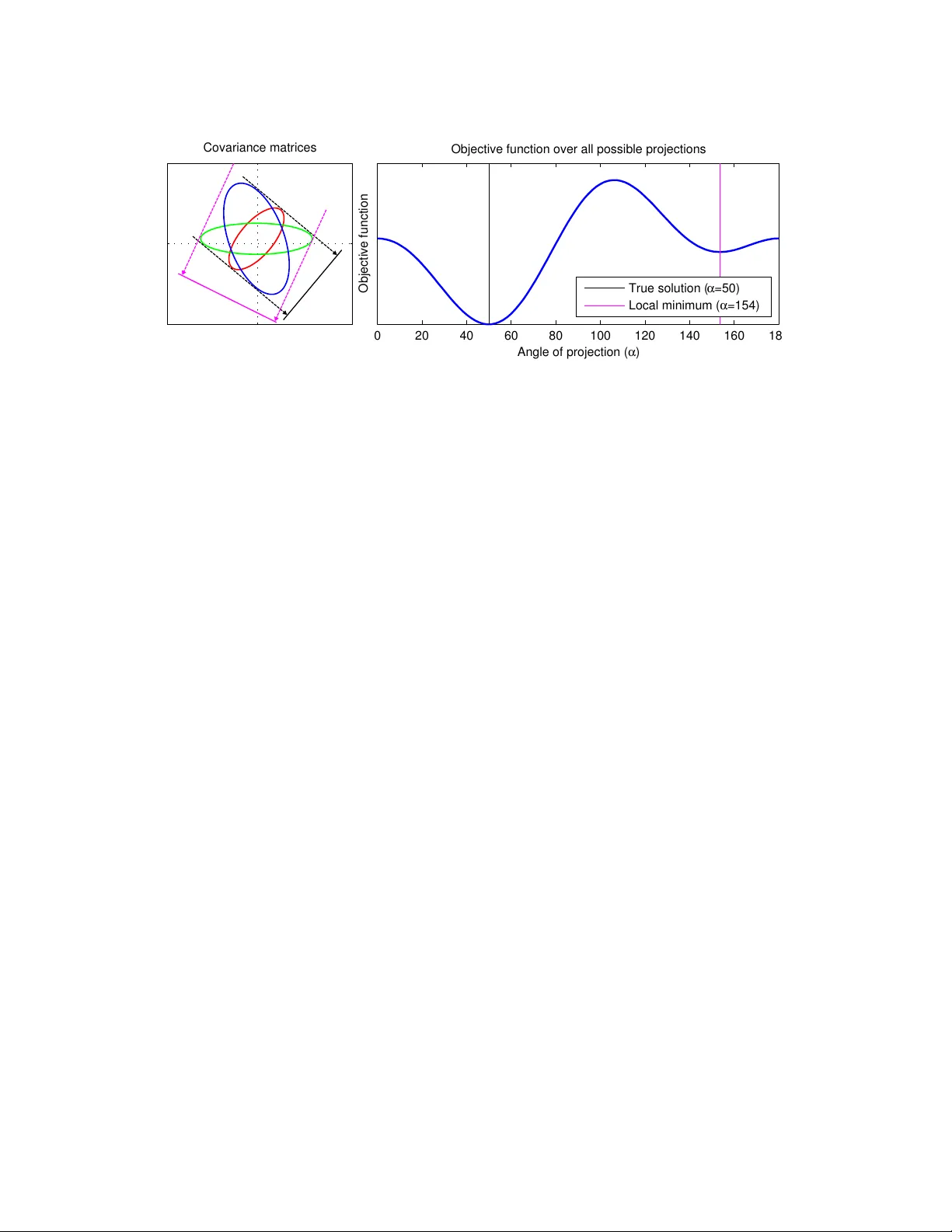
Journal of Machine Learning Research 1 (2011) 1-48 Submitted 4/17; Published 5/42 Algebraic Geometric Comparison of Probabilit y Distributions F ranz J. Kir´ aly franz.j.kiral y@tu-berlin.de Machine L e arning Gr oup, Computer Scienc e Berlin Institute of T e chnolo gy (TU Berlin) F r anklinstr. 28/29, 10587 Berlin, Germany and Discr ete Ge ometry Gr oup, Institute of Mathematics, FU Berlin P aul v on B ¨ unau p aul.buena u@tu-berlin.de F rank C. Meinec k e frank.meinecke@tu-berlin.de Machine L e arning Gr oup, Computer Scienc e Berlin Institute of T e chnolo gy (TU Berlin) F r anklinstr. 28/29, 10587 Berlin, Germany Duncan A. J. Blythe duncan.bl ythe@bccn-berlin.de Machine L e arning Gr oup, Computer Scienc e Berlin Institute of T e chnolo gy (TU Berlin) F r anklinstr. 28/29, 10587 Berlin, Germany and Bernstein Center for Computational Neur oscienc e (BCCN), Berlin Klaus-Rob ert M¨ uller klaus-r ober t.mueller@tu-berlin.de Machine L e arning Gr oup, Computer Scienc e Berlin Institute of T e chnolo gy (TU Berlin) F r anklinstr. 28/29, 10587 Berlin, Germany and IP AM, UCLA, L os Angeles, USA Editor: The editor Abstract W e prop ose a no vel algebraic algorithmic framework for dealing with probability distri- butions represented by their cum ulants such as the mean and cov ariance matrix. As an example, w e consider the unsup ervised learning problem of ﬁnding the subspace on whic h sev eral probability distributions agree. Instead of minimizing an ob jective function inv olv- ing the estimated cumulan ts, we show that by treating the cumulan ts as elements of the p olynomial ring we can directly solve the problem, at a low er computational cost and with higher accuracy . Moreo ver, the algebraic viewp oint on probability distributions allo ws us to inv oke the theory of algebraic geometry , which we demonstrate in a compact pro of for an identiﬁabilit y criterion. Keyw ords: Computational algebraic geometry , Appro ximate algebra, Unsupervised Learning c  2011 F ranz J. Kir´ aly , Paul v on B¨ unau, F rank C. Meineck e, Duncan A.J. Blythe and Klaus-Robert M ¨ uller. Kir ´ al y, von B ¨ unau, Meinecke, Bl ythe and M ¨ uller 1. In tro duction Comparing high dimensional probability distributions is a general problem in machine learn- ing, whic h o ccurs in tw o-sample testing (e.g. Hotelling (1932); Gretton et al. (2007)), pro- jection pursuit (e.g. F riedman and T ukey (1974)), dimensionality reduction and feature se- lection (e.g. T orkkola (2003)). Under mild assumptions, probabilit y densities are uniquely determined by their cumulan ts which are naturally interpreted as co eﬃcients of homoge- neous m ultiv ariate p olynomials. Representing probability densities in terms of cumulan ts is a standard tec hnique in learning algorithms. F or example, in Fisher Discriminant Anal- ysis (Fisher, 1936), the class conditional distributions are approximated b y their ﬁrst tw o cum ulants. In this pap er, we tak e this viewp oin t further and work explicitly with polynomials. That is, w e treat estimated cumulan ts not as constants in an ob jective function, but as ob jects that we manipulate algebraically in order to ﬁnd the optimal solution. As an example, we consider the problem of ﬁnding the linear subspace on which sev eral probability distributions are identical: given D -v ariate random v ariables X 1 , . . . , X m , we w ant to ﬁnd the linear map P ∈ R d × D suc h that the pro jected random v ariables ha ve the same probabilit y distribution, P X 1 ∼ · · · ∼ P X m . This amounts to ﬁnding the directions on whic h all pro jected cumulan ts agree. F or the ﬁrst cumulan t, the mean, the pro jection is readily av ailable as the solution of a set of linear equations. F or higher order cumulan ts, we need to solv e p olynomial equations of higher degree. W e present the ﬁrst algorithm that solves this problem explicitly for arbitrary degree, and show ho w algebraic geometry can b e applied to prov e prop erties ab out it. T o clarify the gist of our approac h, let us consider a st ylized example. In order to solv e a learning problem, the con ven tional approach in machine learning is to form ulate an ob jective function, e.g. the log likelihoo d of the data or the empirical risk. Instead of minimizing an ob jective function that inv olves the p olynomials, w e consider the p olynomials as obje cts in their own right and then solve the problem by algebraic manipulations. The adv an tage of the algebraic approac h is that it captures the inherent structure of the problem, which is in general diﬃcult to mo del in an optimization approach. In other words, the algebraic approac h actually solves the problem, whereas optimization se ar ches the space of p ossible solutions guided by an ob jective function that is minimal at the desired solution, but can giv e p o or directions outside of the neigh b orho o d around its global minimum. Let us consider the problem where w e would like to ﬁnd the direction v ∈ R 2 on which several sample co v ariance matrices Σ 1 , . . . , Σ m ⊂ R 2 × 2 are equal. The usual ansatz w ould b e to formulate an optimization problem such as v ∗ = argmin k v k =1 X 1 ≤ i,j ≤ m  v > Σ i v − v > Σ j v  2 . (1) This ob jective function measures the deviation from equality for all pairs of co v ariance matrices; it is zero if and only if all pro jected co v ariances are equal and p ositiv e otherwise. Figure 1 sho ws an example with three cov ariance matrices (left panel) and the v alue of the ob jective function for all p ossible pro jections v =  cos( α ) sin( α )  > . The solution to 2 Algebraic Geometric Comp arison of Probability Distributions 0 2 0 4 0 6 0 8 0 1 0 0 1 2 0 1 4 0 1 6 0 1 8 0 O b j e c t i v e f u n c t i o n A n g l e o f p r o j e c t i o n ( α ) O b j e c t i v e f u n c t i o n o v e r a l l p o s s i b l e p r o j e c t i o n s C o v a r i a n c e m a t r i c e s T r u e s o l u t i o n ( α = 5 0 ) L o c a l m i n i m u m ( α = 1 5 4 ) Figure 1: Illustration of the optimization approach. The left panel shows the con tour plots of three sample co v ariance matrices. The black line is the true one-dimensional subspace on whic h the pro jected v ariances are exactly equal, the magenta line corresp onds to a lo cal minim um of the ob jective function. The righ t panel shows the v alue of the ob jectiv e function ov er all p ossible one-dimensional subspaces, parameterized b y the angle α to the horizontal axis; the angles corresp onding to the global minim um and the lo cal minim um are indicated b y black and magenta lines resp ectively . this non-conv ex optimization problem can b e found using a gradien t-based searc h pro cedure, whic h may terminate in one of the lo cal minima (e.g. the magenta line in Figure 1) dep ending on the initialization. Ho wev er, the natural representation of this problem is not in terms of an ob jective function, but rather a system of equations to b e solved for v , namely v > Σ 1 v = · · · = v > Σ m v . (2) In fact, b y going from an algebraic description of the set of solutions to a formulation as an optimization problem in Equation 1, w e lose imp ortant structure. In the case where there is an exact solution, it can b e attained explicitly with algebraic manipulations. How ever, when w e estimate a co v ariance matrix from ﬁnite or noisy samples, there exists no exact solution in general. Therefore we present an algorithm whic h combines the statistical treatment of uncertain ty in the coeﬃcients of p olynomials with the exactness of algebraic computations to obtain a consistent estimator for v that is computationally eﬃcient. Note that this approach is not limited to this particular learning task. In fact, it is applicable whenever a set of solutions can b e describ ed in terms of a set of p olynomial equations, which is a rather general setting. F or example, we could use a similar strategy to ﬁnd a subspace on which the pro jected probability distribution has another prop ert y that can b e describ ed in terms of cumulan ts, e.g. indep endence b et ween v ariables. Moreo ver, an algebraic approac h may also b e useful in solving certain optimization problems, as the set of extrema of a p olynomial ob jective function can b e describ ed by the v anishing set of its gradient. The algebraic viewp oint also allows a nov el interpretation of algorithms op erating in the feature space asso ciated with the p olynomial k ernel. W e w ould therefore 3 Kir ´ al y, von B ¨ unau, Meinecke, Bl ythe and M ¨ uller argue that metho ds from computational algebra and algebraic geometry are useful for the wider machine learning comm unity . Figure 2: Representation of the problem: the left panel sho ws sample co v ariance matrices Σ 1 and Σ 2 with the desired pro jection v . In the middle panel, this pro jection is deﬁned as the solution to a quadratic p olynomial. This p olynomial is embedded in the vector space of co eﬃcients spanned b y the monomials X 2 , Y 2 and X Y sho wn in the right panel. Let us ﬁrst of all explain the representation ov er whic h w e compute. W e will pro ceed in the three steps illustrated in Figure 2, from the geometric in terpretation of sample cov ariance matrices in data space (left panel), to the quadratic equation deﬁning the pro jection v (middle panel), to the representation of the quadratic equation as a c o eﬃcien t vector (righ t panel). T o start with, w e consider the Equation 2 as a set of homogeneous quadratic equations deﬁned by v > (Σ i − Σ j ) v = 0 ∀ 1 ≤ i, j ≤ m, (3) where we interpret the comp onen ts of v as v ariables, v =  X Y  > . The solution to these equations is the direction in R 2 on which the pro jected v ariance is equal ov er all cov ariance matrices. Each of these equations corresp onds to a quadratic p olynomial in the v ariables X and Y , q ij = v > (Σ i − Σ j ) v = v >  a 11 a 12 a 21 a 22  v = a 11 X 2 + ( a 12 + a 21 ) X Y + a 22 Y 2 , (4) whic h w e em b ed in to the vector space of coeﬃcients. The coordinate axis are the monomials { X 2 , X Y , Y 2 } , i.e. the three indep endent en tries in the Gram matrix (Σ i − Σ j ). That is, the p olynomial in Equation 4 b ecomes the co eﬃcient vector ~ q ij =  a 11 a 12 + a 21 a 22  > . 4 Algebraic Geometric Comp arison of Probability Distributions The motiv ation for the vector space in terpretation is that every linear combination of the Equations 3 is also a characterization of the set of solutions: this will allo w us to ﬁnd a particular set of equations b y linear com bination, from which we can directly obtain the solution. Note, ho wev er, that the vector space represen tation do es not give us all equations whic h can b e used to describ e the solution: we can also m ultiply with arbitrary p olynomials. Ho wev er, for the algorithm that we present here, linear com binations of p olynomials are suﬃcien t. Figure 3: Illustration of the algebraic algorithm. The left panel sho ws the v ector space of co eﬃcien ts where the p olynomials corresp onding to the Equations 3 are consid- ered as elemen ts of the v ector space shown as red points. The middle panel sho ws the appro ximate 2-dimensional subspace (blue surface) onto whic h we pro ject the p olynomials. The right panel shows the one-dimensional intersection (orange line) of the approximate subspace with the plane spanned by spanned b y { X Y , Y 2 } . This subspace is spanned b y the p olynomial Y ( αX + β Y ), so we can divide b y the v ariable Y . Figure 3 illustrates ho w the algebraic algorithm works in the v ector space of co eﬃcients. The p olynomials Q = { q ij } n i,j =1 span a space of constrain ts which deﬁnes the set of solu- tions. The next step is to ﬁnd a p olynomial of a certain form that immediately reveals the solution. One of these sets is the linear subspace spanned by the monomials { X Y , Y 2 } : an y p olynomial in this span is divisible by Y . Our goal is no w to ﬁnd a p olynomial which is contained in b oth this subspace and the span of Q . Under mild assumptions, one can alw ays ﬁnd a p olynomial of this form, and it corresp onds to an equation Y ( αX + β Y ) = 0 . (5) Since this p olynomial is in the span of Q , our solution v has to b e a zero of this particular p olynomial: v 2 ( αv 1 + β v 2 ) = 0. Moreov er, we can assume 1 that v 2 6 = 0, so that w e can divide out the v ariable Y to get the linear factor ( α X + β Y ), 0 = αX + β Y =  α β  v . 1. This is a consequence of the generative mo del for the observed p olynomials whic h is in tro duced in Section 2.1. In essence, we use the fact that our polynomials ha ve no sp ecial property (apart from the existence of a solution) with probability one. 5 Kir ´ al y, von B ¨ unau, Meinecke, Bl ythe and M ¨ uller Hence v =  − β α  > is the solution up to arbitrary scaling, which corresp onds to the one- dimensional subspace in Figure 3 (orange line, righ t panel). A more detailed treatment of this example can also b e found in App endix A. In the case where there exists a direction v on which the pro jected cov ariances are ex- actly equal, the linear subspace spanned b y the set of polynomials Q has dimension t wo, whic h corresp onds to the degrees of freedom of p ossible cov ariance matrices that ha v e ﬁxed pro jection on one direction. Ho wev er, since in practice co v ariance matrices are estimated from ﬁnite and noisy samples, the polynomials Q usually span the whole space, whic h means that there exists only a trivial solution v = 0. This is the case for the polynomials pictured in the left panel of Figure 3. Thus, in order to obtain an appro ximate solution, w e ﬁrst de- termine the appro ximate tw o-dimensional span of Q using a standard least squares metho d as illustrated in the middle panel. W e can then ﬁnd the intersection of the approximate t wo-dimensional span of Q with the plane spanned b y the monomials { X Y , Y 2 } . As w e ha ve seen in Equation 5, the polynomials in this span provide us with a unique solution for v up to scaling, corresp onding to the fact that the intersection has dimension one (see the righ t panel of Figure 3). Alternativ ely , we could ha ve found the one-dimensional intersection with the span of { X Y , X 2 } and divided out the v ariable X . In fact, in the ﬁnal algorithm we will ﬁnd all such in tersections and combine the solutions in order to increase the accuracy . Note that w e ha ve found this solution by solving a simple least-squares problem (second step, middle panel of Figure 3). In con trast, the optimization approach (Figure 1) can require a large num b er of iterations and may conv erge to a lo cal minimum. A more detailed example of the algebraic algorithm can b e found in App endix A. Figure 4: The left panel sho ws t wo sample cov ariance matrices in the plane, along with a direction on which they are equal. In the right panel, a third (green) cov ariance matrix do es not hav e the same pro jected v ariance on the black direction. The algebraic framew ork do es not only allow us to construct eﬃcient algorithms for w orking with probabilit y distributions, it also oﬀers p ow erful to ols to pro ve properties of algorithms that op erate with cum ulants. F or example, we can answ er the follo wing central question: how many distinct data sets do we need such that the subspace with identical probabilit y distributions b ecomes uniquely iden tiﬁable? This dep ends on the n umber of dimensions and the cum ulants that we consider. Figure 4 illustrates the case where we are giv en only the second order momen t in t wo dimensions. Unless Σ 1 − Σ 2 is indeﬁnite, there always exists a direction on which t wo cov ariance matrices in tw o dimensions are equal (left panel of Figure 4) — irresp ective of whether the probabilit y distributions are actually equal. W e therefore need at least three co v ariance matrices (see righ t panel), or to 6 Algebraic Geometric Comp arison of Probability Distributions consider other cum ulan ts as well. W e deriv e a tigh t criterion on the necessary n umber of data sets dep ending on the dimension and the cum ulants under consideration. The proof hinges on viewing the cumulan ts as p olynomials in the algebraic geometry framework: the p olynomials that deﬁne the sought-after pro jection (e.g. Equations 3) generate an ideal in the p olynomial ring which corresp onds to an algebraic set that contains all p ossible solutions. W e can then show how many indep enden t p olynomials are necessary so that the dimension of the linear part of the algebraic set has smaller dimension in the generic case. W e conjecture that these pro of tec hniques are also applicable to other scenarios where w e aim to identify a prop erty of a probability distribution from its cumulan ts using algebraic metho ds. Our work is not the ﬁrst that applies geometric or algebraic metho ds to Machine Learn- ing or statistics: for example, metho ds from group theory hav e already found their applica- tion in mac hine learning, e.g. Kondor (2007); Kondor and Borgw ardt (2008); there are also algebraic metho ds estimating structured manifold mo dels for data p oints as in Vidal et al. (2005) which are strongly related to p olynomial kernel PCA — a metho d which can itself b e interpreted as a w ay of ﬁnding an approximate v anishing set. The ﬁeld of Information Geometry interprets parameter spaces of probability distribu- tions as diﬀerentiable manifolds and studies them from an information-theoretical p oint of view (see for example the standard b o ok by Amari and Nagaok a (2000)), with recent inter- pretations and improv ements stemming from the ﬁeld of algebraic geometry by W atanab e (2009). There is also the nascent ﬁeld of algebraic statistics whic h studies the parameter spaces of mainly discrete random v ariables in terms of comm utative algebra and algebraic geometry , see the recent ov erviews b y (Sturmfels, 2002, c hapter 8) and Drton et al. (2010) or the b o ok b y Gibilisco et al. (2010) whic h also fo cuses on the interpla y b etw een information geometry and algebraic statistics. These approaches ha ve in common that the algebraic and geometric concepts arise naturally when considering distributions in parameter space. Giv en samples from a probabilit y distribution, we may also consider algebraic structures in the data space. Since the data are uncertain, the algebraic ob jects will also come with an inherent uncertain ty , unlik e the exact manifolds in the case when w e ha ve an a-priori family of probability distributions. Coping with uncertain ties is one of the main interests of the emerging ﬁelds of appro ximative and numerical commutativ e algebra, see the b o ok b y Stetter (2004) for an o verview on numerical metho ds in algebra, and (Kreuzer et al., 2009) for recent dev elopments in approximate techniques on noisy data. There exists a wide range of metho ds; ho w ever, to our kno wledge, the link b etw een approximate algebra and the representation of probability distributions in terms of their cumulan ts has not b een studied yet. The remainder of this paper is organized as follows: in the next Section 2, we in tro- duce the algebraic view of probability distribution, rephrase our problem in terms of this framew ork and inv estigate its identiﬁabilit y . The algorithm for the exact case is presented in Section 3, follow ed by the approximate version in Section 4. The results of our numeri- cal sim ulations and a comparison against Stationary Subspace Analysis (SSA) (v on B ¨ unau et al., 2009) can b e found in Section 5. In the last Section 6, we discuss our ﬁndings and p oin t to future directions. The app endix contains an example and pro of details. 7 Kir ´ al y, von B ¨ unau, Meinecke, Bl ythe and M ¨ uller 2. The Algebraic View on Probabilit y Distributions In this section we introduce the algebraic framew ork for dealing with probability distribu- tions. This requires basic concepts from complex algebraic geometry . A comprehensive in- tro duction to algebraic geometry with a view to computation can be found in the bo ok (Co x et al., 2007). In particular, we recommend to go through the Chapters 1 and 4. In this section, we demonstrate the algebraic viewp oint of probabilit y distributions on the application that w e study in this paper: ﬁnding the linear subspace on whic h probabilit y distributions are equal. Problem 2.1 L et X 1 , . . . , X m b e a set of D -variate r andom variables, having smo oth den- sities. Find al l line ar maps P ∈ R d × D such that the tr ansforme d r andom variables have the same distribution, P X 1 ∼ · · · ∼ P X m . In the ﬁrst part of this section, w e show how this problem can b e formulated algebraically . W e will ﬁrst of all review the relationship b et ween the probabilit y density function and its cum ulants, b efore w e translate the cumulan ts into algebraic ob jects. Then w e introduce the theoretical underpinnings for the statistical treatmen t of p olynomials arising from estimated cum ulants and pro ve conditions on iden tiﬁability for the problem addressed in this pap er. 2.1 F rom Probabilit y Distributions to P olynomials The probabilit y distribution of ev ery smo oth real random v ariable X can b e fully character- ized in terms of its cumulants , whic h are the tensor co eﬃcients of the cumulan t generating function. This represen tation has the adv an tage that eac h cumulan t provides a compact description of certain asp ects of the probability densit y function. Deﬁnition 2.2 L et X b e a D -variate r andom variable. Then by κ n ( X ) ∈ R D ( × n ) we denote the n -th cumulant, which is a r e al tensor of de gr e e n . Let us introduce a useful shorthand notation for linearly transforming tensors. Deﬁnition 2.3 L et A ∈ C d × D b e a matrix. F or a tensor T ∈ R D ( × n ) (i.e. a r e al tensor T of de gr e e n of dimension D n = D · D · . . . · D ) we wil l denote by A ◦ T the applic ation of A to T along al l tensor dimensions, i.e. ( A ◦ T ) i 1 ...i n = D X j 1 =1 · · · D X j n =1 A i 1 j 1 · . . . · A i n j n T j 1 ...j n . The cumulan ts of a linearly transformed random v ariable are the multilinearly transformed cum ulants, whic h is a conv enien t prop erty when one is looking for a certain linear subspace. Prop osition 2.4 L et X b e a r e al D -dimensional r andom variable and let A ∈ R d × D b e a matrix. Then the cumulants of the tr ansforme d r andom variable AX ar e the tr ansforme d cumulants, κ n ( AX ) = A ◦ κ n ( X ) . 8 Algebraic Geometric Comp arison of Probability Distributions W e now w ant to formulate our problem in terms of cum ulants. First of all, note that P X i ∼ P X j if and only if v X i ∼ v X j for all row v ectors v ∈ span P > . Problem 2.5 Find al l d -dimensional line ar subsp ac es in the set of ve ctors S = { v ∈ R D    v > X 1 ∼ · · · ∼ v > X m } = { v ∈ R D    v > ◦ κ n ( X i ) = v > ◦ κ n ( X j ) , n ∈ N , 1 ≤ i, j ≤ m } . Note that w e are lo oking for linear subspaces in S , but that S itself is not a vector space in general. Apart from the fact that S is homogeneous, i.e. λS = S for all λ ∈ R , there is no additional structure that we utilize. F or the sake of clarity , in the remainder of this paper w e restrict ourselves to the ﬁrst t w o cum ulants. Note, how ever, that one of the strengths of the algebraic framework is that the generalization to arbitrary degree is straigh tforw ard; throughout this pap er, we indicate the necessary changes and diﬀerences. Th us, from now on, w e denote the ﬁrst t wo cumulan ts b y µ i = κ 1 ( X i ) and Σ i = κ 2 ( X i ) resp ectively for all 1 ≤ i ≤ m . Moreov er, without loss of generalit y , w e can shift the mean vectors and choose a basis suc h that the random v ariable X m has zero mean and unit cov ariance. Th us we arriv e at the following formulation. Problem 2.6 Find al l d -dimensional line ar subsp ac es in S = { v ∈ R D | v > (Σ i − I ) v = 0 , v > µ i = 0 , 1 ≤ i ≤ ( m − 1) } . Note that S is the set of solutions to m − 1 quadratic and m − 1 linear equations in D v ariables. No w it is only a formal step to arrive in the framework of algebraic geometry: let us think of the left hand side of each of the quadratic and linear equations as p olynomials q 1 , . . . , q m − 1 and f 1 , . . . , f m − 1 in the v ariables T 1 , . . . , T D resp ectiv ely , q i =  T 1 · · · T D  ◦ (Σ i − I ) and f i =  T 1 · · · T D  ◦ µ i , whic h are elemen ts of the p olynomial ring ov er the complex num b ers in D v ariables, C [ T 1 , . . . , T D ]. Note that in the in tro duction we hav e used X and Y to denote the v ari- ables in the p olynomials, w e will now switch to T 1 , . . . , T D in order to a void confusion with random v ariables. Thus S can b e rewritten in terms of p olynomials, S =  v ∈ R D | q i ( v ) = f i ( v ) = 0 ∀ 1 ≤ i ≤ m − 1 } , whic h means that S is an algebraic set. In the following, we will consider the corresp onding complex v anishing set S = V( q 1 , . . . , q m − 1 , f 1 , . . . , f m − 1 ) :=  v ∈ C D | q i ( v ) = f i ( v ) = 0 ∀ 1 ≤ i ≤ m − 1 } ⊆ C D and keep in mind that even tually we will b e interested in the real part of S . W orking ov er the complex n umbers simpliﬁes the theory and creates no algorithmic diﬃculties: when w e start with real cumulan t p olynomials, the solution will alw ays b e real. Finally , we can translate our problem into the language of algebraic geometry . 9 Kir ´ al y, von B ¨ unau, Meinecke, Bl ythe and M ¨ uller Problem 2.7 Find al l d -dimensional line ar subsp ac es in the algebr aic set S = V( q 1 , . . . , q m − 1 , f 1 , . . . , f m − 1 ) . So far, this problem formulation do es not include the assumption that a solution exists. In order to pro v e prop erties about the problem and algorithms for solving it w e need to assume that there e xist a d -dimensional linear subspace S 0 ⊂ S . That is, we need to formulate a gener ative mo del for our observed p olynomials q 1 , . . . , q m − 1 , f 1 , . . . , f m − 1 . T o that end, we in tro duce the concept of a generic p olynomial, for a technical deﬁnition see App endix B. In tuitively , a generic polynomial is a contin uous, p olynomial v alued random v ariable which almost surely has no algebraic prop erties except for those that are logically implied by the conditions on it. An algebraic prop erty is an even t in the probability space of p olynomials whic h is deﬁned by the common v anishing of a set of p olynomial equations in the co eﬃcients. F or example, the prop ert y that a quadratic p olynomial is a square of linear p olynomial is an algebraic prop erty , since it is describ ed b y the v anishing of the discriminants. In the con text of Problem 2.7, we will consider the observ ed p olynomials as generic conditioned on the algebraic prop erty that they v anish on a ﬁxed d -dimensional linear subspace S 0 . One w ay to obtain generic p olynomials is to replace co eﬃcients with e.g. Gaussian random v ariables. F or example, a generic homogeneous quadric q ∈ C [ T 1 , T 2 ] is given b y q = Z 11 T 2 1 + Z 12 T 1 T 2 + Z 22 T 2 2 , where the co eﬃcien ts Z ij ∼ N ( µ ij , σ ij ) are indep enden t Gaussian random v ariables with arbitrary parameters. Apart from being homogeneous, there is no condition on q . If w e w ant to add the condition that q v anishes on the linear space deﬁned by T 1 = 0, we w ould instead consider q = Z 11 T 2 1 + Z 12 T 1 T 2 . A more detailed treatmen t of the concept of genericity , ho w it is linked to probabilistic sampling, and a comparison with the classical deﬁnitions of genericity can b e found in App endix B.1. W e are now ready to reformulate the genericity conditions on the random v ariables X 1 , . . . , X m in the ab ov e framework. Namely , we hav e assumed that the X i are general under the condition that they agree in the ﬁrst t wo cum ulants when pro jected on to some linear subspace S 0 . Rephrased for the cumulan ts, Problems 2.1 and 2.7 b ecome well-posed and can b e formulated as follows. Problem 2.8 L et S 0 b e an unknown d -dimensional line ar subsp ac e in C D . Assume that f 1 , . . . , f m − 1 ar e generic homo genous line ar p olynomials, and q 1 , . . . , q m − 1 ar e generic ho- mo genous quadr atic p olynomials, al l vanishing on S 0 . Find al l d -dimensional line ar sub- sp ac es in the algebr aic set S = V( q 1 , . . . , q m − 1 , f 1 , . . . , f m − 1 ) . As we hav e deﬁned “generic” as an implicit “almost sure” statemen t, we are in fact lo oking for an algorithm whic h giv es the correct answer with probability one under our mo del assumptions. Intuitiv ely , S 0 should b e also the only d -dimensional linear subspace in S , whic h is not immediately guaran teed from the problem description. Indeed this is true if m is large enough, whic h is the topic of the next section. 10 Algebraic Geometric Comp arison of Probability Distributions 2.2 Iden tiﬁabilit y In the last subsection, we hav e seen how to reform ulate our initial Problem 2.1 ab out comparison of cum ulan ts as the completely algebraic Problem 2.8. W e can also reformulate iden tiﬁability of the true solution in the original problem in an algebraic w ay: iden tiﬁability in Problem 2.1 means that the pro jection P can b e uniquely computed from the probability distributions. F ollo wing the same reasoning we used to arrive at the algebraic form ulation in Problem 2.8, one concludes that identiﬁabilit y is equiv alent to the fact that there exists a unique linear subspace in S . Since iden tiﬁability is no w a completely algebraic statemen t, it can b e treated also in algebraic terms. In App endix B, we giv e an algebraic geometric criterion for identiﬁabilit y of the stationary subspace; w e will sk etch its deriv ation in the following. The main ingredien t is the fact that, intuitiv ely sp oken, ev ery generic p olynomials carries one degree of freedom in terms of dimension, as for example the follo wing result on generic v ector spaces sho ws: Prop osition 2.9 L et P b e an algebr aic pr op erty such that the p olynomials with pr op erty P form a ve ctor sp ac e V . L et f 1 , . . . , f n ∈ C [ T 1 , . . . T D ] b e generic p olynomials satisfying P . Then rank span( f 1 , . . . , f n ) = min( n, dim V ) . Pro of This is Prop osition B.14 in the app endix. On the other hand, if the p olynomials act as constrain ts, one can pro ve that eac h one reduces the degrees of freedom in the solution b y one: Prop osition 2.10 L et Z b e a sub-ve ctor sp ac e of C D . L et f 1 , . . . , f n b e generic homo genous p olynomials in D variables (of ﬁxe d, but arbitr ary de gr e e e ach), vanishing on Z . Then for their c ommon vanishing set V ( f 1 , . . . , f n ) = { x ∈ C D | f i ( x ) = 0 ∀ i } , one c an write V( f 1 , . . . , f n ) = Z ∪ U, wher e U is an algebr aic set with dim U ≤ max( D − n, 0) . Pro of This follows from Corollary B.32 in the app endix. Prop osition 2.10 can now b e directly applied to Problem 2.8. It implies that S = S 0 if 2( m − 1) ≥ D + 1, and that S 0 is the maximal dimensional comp onent of S if 2( m − 1) ≥ D − d + 1. That is, if we start with m random v ariables, then S 0 can be iden tiﬁed uniquely if 2( m − 1) ≥ D − d + 1 with classical algorithms from computational algebraic geometry in the noiseless case. Theorem 2.11 L et X 1 , . . . , X m b e r andom variables. Assume ther e exists a pr oje ction P ∈ R d × D such that the ﬁrst two cumulants of al l P X 1 , . . . , P X m agr e e and the cumulants 11 Kir ´ al y, von B ¨ unau, Meinecke, Bl ythe and M ¨ uller ar e generic under those c onditions. Then the pr oje ction P is identiﬁable fr om the ﬁrst two cumulants alone if m ≥ D − d + 1 2 + 1 . Pro of This is a direct consequence of Prop osition B.36 in the app endix, applied to the reform ulation giv en in Problem 2.8. It is obtained by applying Prop osition 2.10 to the generic forms v anishing on the ﬁxed linear subspace S 0 , and using that S 0 can be identiﬁed in S if it is the biggest dimensional part. W e hav e seen that identiﬁabilit y means that there is an algorithm to compute P uniquely when the cum ulan ts are kno wn, resp. to compute a unique S from the polynomials f i , q i . It is not diﬃcult to see that an algorithm doing this can b e made into a consistent estimator when the cum ulants are sample estimates. W e will give an algorithm of this type in the follo wing parts of the pap er. 3. An Algorithm for the Exact Case In this section we presen t an algorithm for solving Problem 2.8, under the assumption that the cum ulants are kno wn exactly . W e will ﬁrst ﬁx notation and in tro duce important algebraic concepts. In the previous section, we deriv ed in Problem 2.8 an algebraic form u- lation of our task: given generic quadratic p olynomials q 1 , . . . , q m − 1 and linear polynomials f 1 , . . . , f m − 1 , v anishing on a unknown linear subspace S 0 of C D , ﬁnd S 0 as the unique d - dimensional linear subspace in the algebraic set V( q 1 , . . . , q m − 1 , f 1 , . . . , f m − 1 ). First of all, note that the linear equations f i can easily be remo ved from the problem: instead of lo oking at C D , we can consider the linear subspace deﬁned b y the f i , and examine the algebraic set V( q 0 1 , . . . , q 0 m − 1 ) , where q 0 i are p olynomials in D − m + 1 v ariables which w e obtain by substi- tuting m − 1 v ariables. So the problem w e need to examine is in fact the mo diﬁed problem where we hav e only quadratic p olynomials. Secondly , we will assume that m − 1 ≥ D . Then, from Proposition 2.10, we know that S = S 0 and Problem 2.8 b ecomes the following. Problem 3.1 L et S b e an unknown d -dimensional subsp ac e of C D . Given m − 1 ≥ D generic homo genous quadr atic p olynomials q 1 , . . . , q m − 1 vanishing on S , ﬁnd the d -dimensional line ar subsp ac e S = V( q 1 , . . . , q m − 1 ) . Of course, w e hav e to say what we mean by ﬁnding the solution. By assumption, the quadratic p olynomials already fully describ e the linear space S . Ho wev er, since S is a linear space, we wan t a basis for S , consisting of d linearly indep endent vectors in C D . Or, equiv alently , w e w ant to ﬁnd linearly indep endent linear forms ` 1 , . . . , ` D − d suc h that ` i ( x ) = 0 for all x ∈ S. The latter is the correct description of the solution in algebraic terms. W e now sho w how to reformulate this in the right language, following the algebra-geometry dualit y . The algebraic set S corresp onds to an ideal in the p olynomial ring C [ T 1 , . . . , T D ]. Notation 3.2 We denote the p olynomial ring C [ T 1 , . . . , T D ] by R . The ide al of S is an ide al in R , and we denote it by by s = I( S ) . Sinc e S is a line ar sp ac e, ther e exists a line ar gener ating set ` 1 , . . . , ` D − d of s which we wil l ﬁx in the fol lowing. 12 Algebraic Geometric Comp arison of Probability Distributions W e can no w relate the Problem 3.1 to a classical problem in algebraic geometry . Problem 3.3 L et m > D and q 1 , . . . , q m − 1 b e generic homo genous quadr atic p olynomials vanishing on a line ar d -dimensional subsp ac e S ⊆ C D . Then ﬁnd a line ar b asis for the r adic al ide al p h q 1 , . . . , q m − 1 i = I(V ( q 1 , . . . , q m − 1 )) = I( S ) . The ﬁrst equalit y follows from Hilbert’s Nullstellensatz. This also sho ws that solving the problem is in fact a question of computing a radical of an ideal. Computing the radical of an ideal is a classical problem in computational algebraic geometry , which is kno wn to b e diﬃcult (for a more detailed discussion see Section 3.3). Ho wev er, if w e assume m − 1 ≥ D ( D + 1) / 2 − d ( d + 1) / 2, we can dramatically reduce the computational cost and it is straigh tforward to derive an approximate solution. In this case, the q i generate the vector space of homogenous quadratic p olynomials whic h v anish on S , which w e will denote b y s 2 . That this is indeed the case, follows from Prop osition 2.9, and we hav e dim s 2 = D ( D + 1) / 2 − d ( d + 1) / 2 , as we will calculate in Remark 3.12. Before we contin ue with solving the problem, w e will need to introduce several concepts and abbreviating notations. First w e in tro duce notation to denote sub-vector spaces whic h con tain p olynomials of certain degrees. Notation 3.4 L et I b e a sub- C -ve ctor sp ac e of R , i.e. I = R , or I is some ide al of R , e.g. I = s . We denote the sub- C -ve ctor sp ac e of homo genous p olynomials of de gr e e k in I by I k (in c ommutative algebr a, this is standar d notation for homo genously gener ate d R -mo dules). F or example, the homogenous p olynomials of degree 2 v anishing on S form exactly the v ector space s 2 . Moreov er, for an y I , the equation I k = I ∩ R k holds. The v ector spaces R 2 and s 2 will b e the central ob jects in the following chapters. As we hav e seen, their dimension is given in terms of triangular num b ers, for which w e introduce some notation: Notation 3.5 We wil l denote the n -th triangular numb er by ∆( n ) = n ( n +1) 2 . The last notational ingredient will capture the structure which is imp osed on R k b y the orthogonal decomp osition C D = S ⊕ S ⊥ . Notation 3.6 L et S ⊥ b e the ortho gonal c omplement of S . Denote its ide al by n = I  S ⊥  . Remark 3.7 As n and s ar e homo genously gener ate d in de gr e e one, we have the c alculation rules s k +1 = s k · R 1 and n k +1 = n k · R 1 , ( s 1 ) k = ( s k ) k and ( n 1 ) k = ( n k ) k wher e · is the symmetrize d tensor or outer pr o duct of ve ctor sp ac es (these rules ar e c anoni- c al ly induc e d by the so-c al le d gr ade d structur e of R -mo dules). In terms of ide als, the ab ove de c omp osition tr anslates to R 1 = s 1 ⊕ n 1 . 13 Kir ´ al y, von B ¨ unau, Meinecke, Bl ythe and M ¨ uller Using the ab ove rules and the binomial formula for ide als, this induc es an ortho gonal de- c omp osition R 2 = R 1 · R 1 = ( s 1 ⊕ n 1 ) · ( s 1 ⊕ n 1 ) = ( s 1 ) 2 ⊕ ( s 1 · n 1 ) ⊕ ( n 1 ) 2 = s 1 · ( s 1 ⊕ n 1 ) ⊕ ( n 2 ) 2 = s 1 · R 1 ⊕ ( n 2 ) 2 = s 2 ⊕ ( n 2 ) 2 (and similar de c omp ositions for the higher de gr e e p olynomials R k ). The tensor pro ducts ab ov e can b e directly translated to pro ducts of ideals, as the vector spaces abov e are each generated in a s ingle degree (e.g. s k , n k , are generated homogenously in degree k ). T o express this, we will deﬁne an ideal whic h corresp onds to R 1 : Notation 3.8 We denote the ide al of R gener ate d by al l monomials of de gr e e 1 by m = h T 1 , . . . , T D i . Note that ideal m is generated b y all elemen ts in R 1 . Moreo ver, w e hav e m k = R k for all k ≥ 1. Using m , one can directly translate pro ducts of vector spaces inv olving some R k in to pro ducts of ideals: Remark 3.9 The e quality of ve ctor sp ac es s k = s 1 · ( R 1 ) k − 1 tr anslates to the e quality of ide als s ∩ m k = s · m k − 1 , sinc e b oth the left and right sides ar e homo genously gener ate d in de gr e e k . 3.1 The Algorithm S ⊂ C D d -dimensional pro jection space R = C [ T 1 , . . . T D ] P olynomial ring o ver C in D v ariables R k C -v ector space of homogenous k -forms in T 1 , . . . , T D ∆( n ) = n ( n +1) 2 n -th triangular num b er s = h ` 1 , . . . , ` D − d i = I( S ) The ideal of S , generated by linear p olynomials ` i s k = R k ∩ s C -v ector space of homogenous k -forms v anishing on S n = I( S ⊥ ) The ideal of S ⊥ n k = R k ∩ n C -v ector space of homogenous k -forms v anishing on S ⊥ m = h T 1 , . . . , T D i The ideal of the origin in C D T able 1: Notation and imp ortant deﬁnitions In this section w e presen t an algorithm for solving Problem 3.3, the computation of the radical of the ideal h q 1 , . . . , q m − 1 i under the assumption that m ≥ ∆( D ) − ∆( d ) + 1 . 14 Algebraic Geometric Comp arison of Probability Distributions Under those conditions, as w e will pro ve in Remark 3.12 (iii), we ha ve that h q 1 , . . . , q m − 1 i = s 2 . Using the notations previously deﬁned, one can therefore infer that solving Problem 3.3 is equiv alent to computing the radical s = √ s · m in the sense of obtaining a linear generating set for s , or equiv alen t to ﬁnding a basis for s 1 when s 2 is giv en in an arbitrary basis. s 2 con tains the complete information giv en by the co v ariance matrices and s 1 giv es an explicit linear description of the space of pro jections under which the random v ariables X 1 , . . . , X m agree. Algorithm 1 The input consists of the quadratic forms q 1 , . . . , q m − 1 ∈ R , generating s 2 , and the dimension d ; the output is the linear generating set ` 1 , . . . , ` D − d for s 1 . 1: Let π ← (1 2 · · · D ) b e a transitive permutation of the v ariable indices { 1 , . . . , D } 2: Let Q ←  q 1 · · · q m − 1  > b e the (( m − 1) × ∆( D ))-matrix of co eﬃcient v ectors, where ev ery row corresp onds to a p olynomial and every column to a monomial T i T j . 3: for k = 1 , . . . , D − d do 4: Order the columns of Q according to the lexicographical ordering of monomials T i T j with v ariable indices p erm uted by π k , i.e. the ordering of the columns is given by the relation  as T 2 π k (1)  T π k (1) T π k (2)  T π k (1) T π k (3)  · · ·  T π k (1) T π k ( D )  T 2 π k (2)  T π k (2) T π k (3)  · · ·  T 2 π k ( D − 1)  T π k ( D − 1) T π k ( D )  T 2 π k ( D ) 5: T ransform Q into upper triangular form Q 0 using Gaussian elimination 6: The last non-zero row of Q 0 is a p olynomial T π k ( D ) ` , where ` is a linear form in s , and we set ` k ← ` 7: end for Algorithm 1 shows the pro cedure in pseudo-co de; a summary of the notation deﬁned in the previous section can b e found in T able 1. The algorithm has p olynomial complexity in the dimension d of the linear subspace S . Remark 3.10 Algorithm 1 has aver age and worst c ase c omplexity O  (∆( D ) − ∆( d )) 2 ∆( D )  , In p articular, if d is not c onsider e d as p ar ameter of the algorithm, the aver age and the worst c ase c omplexity is O ( D 6 ) . On the other hand, if ∆( D ) − ∆( d ) is c onsider e d a ﬁxe d p ar ameter, then Algorithm 1 has aver age and worst c ase c omplexity O ( D 2 ) . Pro of This follo ws from the complexities of the elementary op erations: upp er triangu- larization of a generic matrix of rank r with m columns matrix needs O ( r 2 m ) op erations. W e ﬁrst p erform triangularization of a rank ∆( D ) − ∆( d ) matrix with ∆( D ) columns. The p erm utations can b e obtained eﬃciently by bringing Q in row-ec helon form and then p er- forming row op erations. Op erations for extracting the linear forms and comparisons with resp ect to the monomial ordering are negligible. Th us the ov erall op eration complexity to calculate s 1 is O ((∆( D ) − ∆( d )) 2 ∆( D )) . 15 Kir ´ al y, von B ¨ unau, Meinecke, Bl ythe and M ¨ uller Note that the diﬀerence b et ween worst- and av erage case lies at most in the co eﬃ- cien ts, since the inputs are generic and the complexity only dep ends on the parameter D and not on the q i . Th us, with probability 1 , exactly the worst-case-complexit y is attained. There are t wo crucial facts whic h need to b e veriﬁed for correctness of this algorithm. Namely , there are implicit claims made in Line 6 of Algorithm 1: First, it is claimed that the last non-zero ro w of Q 0 corresp onds to a p olynomial which factors in to certain linear forms. Second, it is claimed that the ` obtained in step 6 generate s resp. s 1 . The pro ofs of these non-trivial claims can b e found in Prop osition 3.11 in the next subsection. Dealing with additional linear forms f 1 , . . . , f m − 1 , is p ossible by wa y of a slight mo diﬁ- cation of the algorithm. Because the f i are linear forms, they are generators of s . W e may assume that the f i are linearly indep endent. By p erforming Gaussian elimination b efore the execution of Algorithm 1, we ma y reduce the n umber of v ariables b y m − 1, thus ha ving to deal with new quadratic forms in D − m + 1 instead of D v ariables. Also, the dimension of the space of pro jections is reduced to min( d − m + 1 , − 1) . Setting D 0 = D − m + 1 and d 0 = min( d − m + 1 , − 1) and considering the quadratic forms q i with Gaussian eliminated v ariables, Algorithm 1 can b e applied to the quadratic forms to ﬁnd the remaining genera- tors for s 1 . In particular, if m − 1 ≥ d, then there is no need for considering the quadratic forms, since d linearly indep endent linear forms already suﬃce to determine the solution. W e can also incorp orate forms of higher degree corresp onding to higher order cum ulants. F or this, we start with s k , where k is the degree of the homogenous polynomials w e get from the cumulan t tensors of higher degree. Supp osing w e start with enough cumulan ts, w e may assume that we hav e a basis of s k . Performing Gaussian elimination on this basis with resp ect to the lexicographical order, we obtain in the last row a form of type T k − 1 π k ( D ) `, where ` is a linear form. Doing this for D − d p erm utations again yields a basis for s 1 . Moreo ver, slight algebraic mo diﬁcations of this strategy also allow to consider data from cumulan ts of diﬀerent degree sim ultaneously , and to reduce the n umber of needed p olynomials to O ( D ); ho wev er, due to its technicalit y , this is b eyond the scop e of the pap er. W e sk etch the idea: In the general case, one starts with an ideal I = h f 1 , . . . , f m i , homogenously generated in arbitrary degrees. suc h that √ I = s . Prop osition in the ap- p endix implies that this happ ens whenever m ≥ D + 1 . One then pro ves that due to the genericit y of the f i , there exists an N suc h that I N = s N , whic h means that s 1 can again b e obtained b y calculating the saturation of the ideal I . When ﬁxing the degrees of the f i , w e will ha ve N = O ( D ) with a relatively small constan t (for all f i quadratic, this even b ecomes N = O ( √ D )). So algorithmically , one w ould ﬁrst calculate I N = s N , which then ma y b e used to compute s 1 and thus s analogously to the case N = 2, as describ ed ab ov e. 16 Algebraic Geometric Comp arison of Probability Distributions 3.2 Pro of of correctness In order to pro ve the correctness of Algorithm 1, we need to prov e the following three statemen ts. Prop osition 3.11 F or Algorithm 1 it holds that (i) Q is of r ank ∆( D ) − ∆( d ) . (ii) The last c olumn of Q in step 6 is of the claime d form. (iii) The ` 1 , . . . , ` D − d gener ate s 1 . Pro of This prop osition will b e prov ed successively in the following: (i) will follo w from Remark 3.12 (iii); (ii) will b e prov ed in Lemma 3.13; and (iii) will b e prov ed in Prop osi- tion 3.14. Let us ﬁrst of all make some observ ations ab out the structure of the v ector space s 2 in whic h w e compute. It is the vector space of p olynomials of homogenous degree 2 v anishing on S . On the other hand, we are lo oking for a basis ` 1 , . . . , ` D − d of s 1 . The follo wing remark will relate b oth vector spaces: Remark 3.12 The fol lowing statements hold: (i) s 2 is gener ate d by the p olynomials ` i T j , 1 ≤ i ≤ D − d, 1 ≤ j ≤ D , . (ii) dim C s 2 = ∆( D ) − ∆( d ) (iii) L et q 1 , . . . , q m with m ≥ ∆( D ) − ∆( d ) b e generic homo genous quadr atic p olynomials in s . Then h q 1 , . . . , q m i = s 2 . Pro of (i) In Remark 3.7, we hav e concluded that s 2 = s 1 · R 1 . Th us the pro duct v ector space s 2 is generated by a pro duct basis of s 1 and R 1 . Since T j , 1 ≤ j ≤ D is a basis for R 1 , and ` i , 1 ≤ i ≤ D − d is a basis for s 1 , the statement holds. (ii) In Remark 3.9, w e hav e seen that R 2 = s 2 ⊕ ( n 1 ) 2 , thus dim s 2 = dim R 2 − dim( n 1 ) 2 . The vector space R 2 is minimally generated by the monomials of degree 2 in T 1 , . . . T D , whose n umber is ∆( D ). Similarly , ( n 1 ) 2 is minimally generated by the monomials of degree 2 in the v ariables ` 0 1 , . . . , ` 0 d that form the dual basis to the ` i . Their num b er is ∆( d ), so the statement follows. (iii) As the q i are homogenous of degree tw o and v anish on S , they are elements in s 2 . Due to (ii), we can apply Prop osition 2.9 to conclude that they generate s 2 as vector space. No w we con tinue to pro ve the remaining claims. Lemma 3.13 In A lgorithm 1 the (∆( D ) − ∆( d )) -th r ow of Q 0 (the upp er triangular form of Q ) c orr esp onds to a 2 -form T π ( D ) ` with a line ar p olynomial ` ∈ s 1 . Pro of Note that ev ery homogenous p olynomial of degree k is canonically an element of the vector space R k in the monomial basis given b y the T i . Thus it makes sense to speak ab out the co eﬃcients of T i for an 1-form resp. the co eﬃcients of T i T j of a 2-form. Also, without loss of generalit y , we can take the trivial p ermutation π = id, since the pro of will not dep end on the c hosen lexicographical ordering and thus will be naturally in- v ariant under p ermutations of v ariables. First w e remark: since S is a generic d -dimensional linear subspace of C D , any linear form in s 1 will ha ve at least d + 1 non-v anishing co eﬃ- cien ts in the T i . On the other hand, by displa ying the generators ` i , 1 ≤ i ≤ D − d in s 1 17 Kir ´ al y, von B ¨ unau, Meinecke, Bl ythe and M ¨ uller in reduced row echelon form with resp ect to the T i -basis, one sees that one can c ho ose all the ` i in fact with exactly d + 1 non-v anishing co eﬃcients in the T i suc h that no non trivial linear combination of the ` i has less then d + 1 non-v anishing coeﬃcients. In particular, one can choose the ` i suc h that the biggest (w.r.t. the lexicographical order) monomial with non-v anishing co eﬃcient of ` i is T i . Remark 3.12 (i) states that s 2 is generated by ` i T j , 1 ≤ i ≤ D − d, 1 ≤ j ≤ D . T ogether with our ab ov e reasoning, this implies the following. F act 1: There exist linear forms ` i , 1 ≤ i ≤ D − d such that: the 2-forms ` i T j generate s 2 , and the biggest monomial of ` i T j with non-v anishing coeﬃcient under the lexicographical ordering is T i T j . By Remark 3.12 (ii), the last row of the upp er triangular form Q 0 is a p olynomial which has zero co eﬃcien ts for all monomials p ossibly except the ∆( d ) + 1 smallest, T D − d T D , T 2 D − d +1 , T D − d +1 T D − d +2 , . . . , T D − 1 T D , T 2 D . On the other hand, it is guaranteed b y our genericity assumption that the biggest of those terms is indeed non-v anishing, which implies the follo wing. F act 2: The biggest monomial of the last row with non-v anishing co eﬃcient (w.r.t the lexicographical order) is that of T D − d T D . Com bining F acts 1 and 2, w e can no w infer that the last ro w m ust be a scalar m ultiple of ` D − d T D : since the last row corresponds to an element of s 2 , it m ust b e a linear combination of the ` i T j . By F act 1, every contribution of an ` i T j , ( i, j ) 6 = ( D − d, D ) w ould add a non- v anishing coeﬃcient lexicographically bigger than T D − d T D whic h cannot cancel. So, b y F act 2, T D divides the last row of the upp er triangular form of Q, which then m ust b e T D ` D − d or a multiple thereof. Also w e hav e that ` D − d ∈ s b y deﬁnition. It remains to b e shown that b y p erm utation of the v ariables w e can ﬁnd a basis for s 1 . Prop osition 3.14 The ` 1 , . . . , ` D − d gener ate s 1 as ve ctor sp ac e and thus s as ide al. Pro of Recall that π i w as the p ermutation to obtain ` i . As w e hav e seen in the pro of of Lemma 3.13, ` i is a linear form which has non-zero co eﬃcients only for the d + 1 coeﬃcients T π i ( D − d ) , . . . , T π i ( D ) . Th us ` i has a non-zero co eﬃcient where all the ` j , j < i hav e a zero co eﬃcien t, and thus ` i is linearly indep endent from the ` j , j < i. In particular, it follows that the ` i are linearly independent in R 1 . On the other hand, they are con tained in the D − d -dimensional sub- C -vector space s 1 and are thus a basis of s 1 , and also a generating set for the ideal s . Note that all of these pro ofs generalize to k -forms. F or example, one calculates that dim C s k =  D + k − 1 k  −  d + k − 1 k  , and the triangularization strategy yields a last row which corresp onds to T k − 1 π ( D ) ` with a linear p olynomial ` ∈ s 1 18 Algebraic Geometric Comp arison of Probability Distributions 3.3 Relation to Previous W ork in Computational Algebraic Geometry In this section, we discuss ho w the algebraic form ulation of the cum ulan t comparison prob- lem given in Problem 3.3 relates to the classical problems in computational algebraic ge- ometry . Problem 3.3 confronts us with the follo wing task: given p olynomials q 1 , . . . , q m − 1 with sp ecial prop erties, compute a linear generating set for the radical ideal p h q 1 , . . . , q m − 1 i = I(V ( q 1 , . . . , q m − 1 )) . Computing the radical of an ideal is a classical task in computational algebraic geometry , so our problem is a special case of radical computation of ideals, which in turn can b e viewed as an instance of primary decomp osition of ideals, see (Cox et al., 2007, 4.7). While it has b een known for long time that there exist constructiv e algorithms to cal- culate the radical of a given ideal in p olynomial rings Hermann (1926), only in the recent decades there hav e been algorithms feasible for implemen tation in mo dern computer alge- bra systems. The b est kno wn algorithms are those of Gianni et al. (1988), implemented in AXIOM and REDUCE, the algorithm of Eisen bud et al. (1992), implemen ted in Macaula y 2, the algorithm of Cab oara et al. (1997), currently implemented in CoCoA, and the al- gorithm of Krick and Logar (1991) and its mo diﬁcation b y Laplagne (2006), a v ailable in SINGULAR. All of these algorithms hav e tw o p oints in common. First of all, these algorithms hav e computational worst case complexities which are doubly exp onential in the square of the n umber of v ariables of the given polynomial ring, see (Laplagne, 2006, section 4.). Although the worst case complexities ma y not b e approached for the problem setting describ ed in the curren t pap er, these oﬀ-the-shelf algorithms do not take in to account the sp eciﬁc prop erties of the ideals in question. On the other hand, Algorithm 1 can b e seen as a homogenous v ersion of the well-kno wn Buc hberger algorithm to ﬁnd a Gro ebner basis of the dehomogenization of s with resp ect to a degree-ﬁrst order. Namely , due to our strong assumptions on m , or as is sho wn in Prop osition B.27 in the appendix for a more general case, the homogenous saturations of the ideal h q 1 , . . . , q m − 1 i = m · s and the ideal s coincide. In particular, the dehomogenizations of the q i constitute a generating set for the dehomogenization of s . The Buch b erger algorithm no w ﬁnds a reduced Groebner basis of s whic h consists of exactly D − d linear polynomials. Their homogenizations then constitute a basis of homogenous linear forms of s itself. It can b e chec ked that the ﬁrst elimination steps whic h the Buch b erger algorithm p erforms for the dehomogenizations of the q i corresp ond directly to the elimination steps in Algorithm 1 for their homogenous versions. So our algorithm p erforms similarly to the Buch b erger algorithm in a noiseless setting, since b oth algorithms compute a reduced Gro ebner basis in the chosen coordinate system. Ho wev er, in our setting which stems from real data, there is a second point which is more gra ve and makes the use of oﬀ-the-shelf algorithms impossible: the computability of an exact result completely relies on the assumption that the ideals given as input are exactly known, i.e. a generating set of p olynomials is exactly known. This is not a problem in classical computational algebra; ho wev er, when dealing with p olynomials obtained from real data, the polynomials come not only with n umerical error, but in fact with statistical uncertain t y . 19 Kir ´ al y, von B ¨ unau, Meinecke, Bl ythe and M ¨ uller In general, the classical algorithms are unable to ﬁnd any solution when confronted ev en with minimal noise on the otherwise exact p olynomials. Namely , when w e deal with a system of equations for whic h ov er-determination is p ossible, any p erturb ed system will b e ov er-determined and th us hav e no solution. F or example, the exact in tersection of N > D + 1 linear subspaces in complex D -space is alwa ys empty when they are sampled with uncertain ty; this is a direct consequence of Proposition 2.10, when using the assumption that the noise is generic. How ever, if all those hyperplanes are nearly the same, then the result of a meaningful approximate algorithm should b e a hyperplane close to all input h yp erplanes instead of the empty set. Before w e con tinue, w e w ould like to stress a conceptual p oint in approac hing uncer- tain ty . First, as in classical n umerics, one can think of the input as theoretically exact, but with ﬁxed error ε and then derive bounds on the output error in terms of this ε and analyze their asymptotics. W e will refer to this approach as numeric al unc ertainty , as opp osed to statistic al unc ertainty , whic h is a view more common to statistics and mac hine learning, as it is more natural for noisy data. Here, the error is considered as inherently probabilistic due to small sample eﬀects or noise ﬂuctuation, and algorithms ma y b e analyzed for their statistical prop erties, indep endent of whether they are themselv es deterministic or sto chas- tic. The statistical view on uncertain t y is the one the reader should hav e in mind when reading this pap er. P arts of the algebra communit y hav e b een committed to the numerical viewp oint on uncertain p olynomials: the problem of n umerical uncertain ty is for example extensively addressed in Stetter’s standard b o ok on numerical algebra (Stetter, 2004). The main dif- ﬁculties and innov ations stem from the fact that standard metho ds from algebra lik e the application of Gro ebner bases are numerically unstable, see (Stetter, 2004, chapter 4.1-2). Recen tly , the algebraic geometry communit y has developed an increasing in terest in solving algebraic problems arising from the consideration of real w orld data. The algorithms in this area are more motiv ated to p erform w ell on the data, some authors start to adapt a statistical viewp oint on uncertain ty , while the inﬂuence of the n umerical view is still dominan t. As a distinction, the authors describ e the ﬁeld as appro ximate algebra instead of numerical algebra. Recen t developmen ts in this sense can b e found for example in (Heldt et al., 2009) or the b o ok of Kreuzer et al. (2009). W e will refer to this viewp oint as the statistical view in order to av oid confusion with other meanings of approximate. In terestingly , there are signiﬁcan t similarities on the metho dological side. Namely , in computational algebra, algorithms often compute primarily ov er vector spaces, whic h arise for example as spaces of polynomials with certain properties. Here, numerical linear algebra can pro vide many tec hniques of enforcing n umerical stability , see the pioneering pap er of Corless et al. (1995). Since then, man y algorithms in numerical and appro ximate algebra utilize linear optimization to estimate vector spaces of p olynomials. In particular, least- squares-appro ximations of rank or kernel are canonical concepts in b oth n umerical and appro ximate algebra. Ho wev er, to the b est of our kno wledge, there is to date no algorithm whic h computes an “approximate” (or “numerical”) radical of an ideal, or an approximate saturation, and also none in our sp ecial case. In the next section, we will use estimation tec hniques from linear algebra to con vert Algorithm 1 in to an algorithm which can cop e with the inherent statistical uncertaint y of the estimation problem. 20 Algebraic Geometric Comp arison of Probability Distributions 4. Approximate Algebraic Geometry on Real Data In this section we sho w how algebraic computations can b e applied to p olynomials with inexact co eﬃcients obtained from estimated cumulan ts on ﬁnite samples. Note that our metho d for computing the approximate radical is not sp eciﬁc to the problem studied in this pap er. The reason why w e cannot directly apply our algorithm for the exact case to estimated p olynomials is that it relies on the assumption that there exists an exact solution, such that the pro jected cumulan ts are equal, i.e. we can ﬁnd a pro jection P such that the equalities P Σ 1 P > = · · · = P Σ m P > and P µ 1 = · · · = P µ m hold exactly . How ev er, when the elements of Σ 1 , . . . , Σ m and µ 1 , . . . , µ m are sub ject to random ﬂuctuations or noise, there exists no pro jection that yields exactly the same ran- dom v ariables. In algebraic terms, w orking with inexact p olynomials means that the joint v anishing set of q 1 , . . . , q m − 1 and f 1 , . . . , f m − 1 consists only of the origin 0 ∈ C D so that the ideal b ecomes trivial: h q 1 , . . . , q m − 1 , f 1 , . . . , f m − 1 i = m . Th us, in order to ﬁnd a meaningful solution, we need to compute the radical appro ximately . In the exact algorithm, we are lo oking for a p olynomial of the form T D ` v anishing on S , whic h is also a C -linear combination of the quadratic forms q i . The algorithm is based on an explicit w ay to do so which works since the q i are generic and suﬃcien t in num b er. So one could pro ceed to adapt this algorithm to the approximate case by p erforming the same op erations as in the exact case and then taking the (∆( D ) − ∆( d ))-th ro w, setting co eﬃcien ts not divisible b y T D to zero, and then dividing out T D to get a linear form. This strategy p erforms fairly w ell for small dimensions D and conv erges to the correct solution, alb eit slowly . Instead of computing one particular linear generator as in the exact case, it is advisable to utilize as m uch information as p ossible in order to obtain b etter accuracy . The least- squares-optimal w ay to approximate a linear space of known dimension is to use singular v alue decomp osition (SVD): with this metho d, w e may directly eliminate the most insignif- ican t directions in co eﬃcien t space which are due to ﬂuctuations in the input. T o that end, w e ﬁrst deﬁne an approximation of an arbitrary matrix by a matrix of ﬁxed rank. Deﬁnition 4.1 L et A ∈ C m × n with singular value de c omp osition A = U DV ∗ , wher e D = diag( σ 1 , . . . , σ p ) ∈ C p × p is a diagonal matrix with or der e d singular values on the diagonal, | σ 1 | ≥ | σ 2 | ≥ · · · ≥ | σ p | ≥ 0 . F or k ≤ p, let D 0 = diag( σ 1 , . . . , σ k , 0 , . . . , 0) . Then the matrix A 0 = U D 0 V ∗ is c al le d r ank k appr oximation of A. The nul l sp ac e, left nul l sp ac e, r ow sp an, c olumn sp an of A 0 wil l b e c al le d r ank k appr oximate nul l sp ac e, left nul l sp ac e, r ow sp an, c olumn sp an of A. F or example, if u 1 , . . . , u p and v 1 , . . . , v p are the columns of U and V resp ectively , the rank k approximate left n ull space of A is spanned b y the rows of the matrix L =  u p − k +1 · · · u p  > , 21 Kir ´ al y, von B ¨ unau, Meinecke, Bl ythe and M ¨ uller and the rank k appro ximate row span of A is spanned by the ro ws of the matrix S =  v 1 · · · v p  > . W e will call those matrices the appr oximate left nul l sp ac e matrix resp. the approximate ro w span matrix of rank k asso ciated to A. The approximate matrices are the optimal appro ximations of rank k with resp ect to the least-squares error. W e can no w use these concepts to obtain an approximativ e version of Algorithm 1. Instead of searc hing for a single elemen t of the form T D `, we estimate the v ector space of all suc h elements via singular v alue decomp osition — note that this is exactly the vector space ( h T D i · s ) 2 , i.e. the vector space of all homogenous p olynomials of degree t w o whic h are divisible by T D . Also note that the c hoice of the linear form T D is irrelev ant, i.e. w e ma y replace T D ab o ve by an y v ariable or ev en linear form. As a trade-oﬀ b etw een accuracy and runtime, w e additionally estimate the v ector spaces ( h T D i · s ) 2 for all 1 ≤ i ≤ D , and then least-squares a verage the putativ e results for s to obtain a ﬁnal estimator for s and th us the desired space of pro jections. Algorithm 2 The input consists of noisy quadratic forms q 1 , . . . , q m − 1 ∈ C [ T 1 , . . . , T D ], and the dimension d ; the output is an approximate linear generating set ` 1 , . . . , ` D − d for the ideal s . 1: Let Q ←  q 1 · · · q m − 1  > b e the ( m − 1 × ∆( D ))-matrix of co eﬃcient vectors, where ev ery row corresp onds to a p olynomial and every column to a monomial T i T j in arbitrary order. 2: for i = 1 , . . . , D do 3: Let Q i b e the (( m − 1) × ∆( D ) − D )-sub-matrix of Q obtained by removing all columns corresp onding to monomials divisible by T i 4: Compute the appro ximate left null space matrix L i of Q i of rank ( m − 1) − ∆( D ) + ∆( d ) + D − d 5: Compute the appro ximate row span matrix L 0 i of L i Q of rank D − d 6: Let L 00 i b e the ( D − d × D )-matrix obtained from L 0 i b y remo ving all columns corre- sp onding to monomials not divisible by T i 7: end for 8: Let L b e the ( D ( D − d ) × D )-matrix obtained by v ertical concatenation of L 00 1 , . . . , L 00 D 9: Compute the approximate ro w span matrix A =  a 1 · · · a D − d  > of L of rank D − d and let ` i =  T 1 · · · T D  a i for all 1 ≤ i ≤ D − d . W e explain the logic b ehind the single steps: In the ﬁrst step, w e start with the same matrix Q as in Algorithm 1. Instead of bringing Q in to triangular form with resp ect to the term order T 1 ≺ · · · ≺ T D , we compute the left k ernel space row matrix S i of the monomials not divisible by T i . Its left image L i = S i Q is a matrix whose ro w space generates the space of p ossible last rows after bringing Q into triangular form in an arbitrary coordinate system. In the next step, we p erform PCA to estimate a basis for the so-obtained v ector space of quadratic forms of type T i times linear form, and extract a basis for the vector space of linear forms estimated via L i . No w we can put together all L i and again p erform PCA to obtain a more exact and numerically more estimate for the pro jection in the last 22 Algebraic Geometric Comp arison of Probability Distributions step. The rank of the matrices after PCA is alw ays c hosen to matc h the correct ranks in the exact case. Note that Algorithm 2 is a consisten t estimator for the correct space of pro jections if the cov ariances are sample estimates. Let us ﬁrst clarify in which sense consistent is mean t here: If each cov ariance matrix is estimated from a sample of size N or greater, and N go es to inﬁnity , then the estimate of the pro jection conv erges in probability to the true pro jection. The reason wh y Algorithm 2 gives a consistent estimator in this sense is elemen tary: co v ariance matrices can b e estimated consisten tly , and so can their diﬀerences, the p olynomials q i . Moreo v er, the algorithm can b e regarded as an almost contin uous function in the p olynomials q i ; so conv ergence in probability to the true pro jection and th us consistency follo ws from the contin uous mapping theorem. The runtime complexity of Algorithm 2 is O ( D 6 ) as for Algorithm 1. F or this note that calculating the singular v alue decomp osition of an m × n -matrix is O ( mn max( m, n )) . If w e wan t to consider k -forms instead of 2-forms, we can use the same strategies as ab o ve to n umerically stabilize the exact algorithm. In the second step, one might w ant to consider all sub-matrices Q M of Q obtained by removing all columns corresp onding to monomials divisible b y some degree ( k − 1) monomial M and p erform the for-lo op o ver all such monomials or a selection of them. Considering D monomials or more giv es again a consistent estimator for the pro jection. Similarly , these metho ds allow us to n umeri- cally stabilize v ersions with reduced ep o c h requirements and simultaneous consideration of diﬀeren t degrees. 5. Numerical Ev aluation In this section w e ev aluate the p erformance of the algebraic algorithm on synthetic data in v arious settings. In order to contrast the algebraic approach with an optimization- based metho d (cf. Figure 1), we compare with the Stationary Subspace Analysis (SSA) algorithm (von B ¨ unau et al., 2009), whic h solv es a similar problem in the con text of time series analysis. T o date, SSA has b een successfully applied in the con text of biomedical data analysis (von B¨ unau et al., 2010), domain adaptation (Hara et al., 2010), change-point detection (von B ¨ unau et al., 2009) and computer vision (Meineck e et al., 2009). 5.1 Stationary Subspace Analysis Stationary Subspace Analysis (von B ¨ unau et al., 2009; M ¨ uller et al., 2011) factorizes an ob- serv ed time series according to a linear model in to underlying stationary and non-stationary sources. The observed time series x ( t ) ∈ R D is assumed to b e generated as a linear mixture of stationary sources s s ( t ) ∈ R d and non-stationary sources s n ( t ) ∈ R D − d , x ( t ) = As ( t ) =  A s A n   s s ( t ) s n ( t )  , (6) with a time-constant mixing matrix A . The underlying sources s ( t ) are not assumed to b e indep enden t or uncorrelated. The aim of SSA is to inv ert this mixing mo del given only samples from x ( t ). The true mixing matrix A is not identiﬁable (von B ¨ unau et al., 2009); only the pro jection P ∈ R d × D 23 Kir ´ al y, von B ¨ unau, Meinecke, Bl ythe and M ¨ uller to the stationary sources can b e estimated from the mixed signals x ( t ), up to arbitrary linear transformation of its image. The estimated stationary sources are given b y ˆ s s ( t ) = P x ( t ), i.e. the pro jection P eliminates all non-stationary con tributions: P A n = 0. The SSA algorithms (v on B¨ unau et al., 2009; Hara et al., 2010) are based on the following deﬁnition of stationarity: a time series X t is considered stationary if its mean and co v ariance is constan t ov er time, i.e. E [ X t 1 ] = E [ X t 2 ] and E [ X t 1 X > t 1 ] = E [ X t 2 X > t 2 ] for all pairs of time p oints t 1 , t 2 ∈ N . F ollo wing this concept of stationarity , the pro jection P is found by minimizing the diﬀerence b etw een the ﬁrst t w o momen ts of the estimated stationary sources ˆ s s ( t ) across ep o chs of the times series. T o that end, the samples from x ( t ) are divided into m non-ov erlapping epo c hs of equal size, corresponding to the index sets T 1 , . . . , T m , from whic h the mean and the cov ariance matrix is es timated for all ep o c hs 1 ≤ i ≤ m , ˆ µ i = 1 |T i | X t ∈T i x ( t ) and ˆ Σ i = 1 |T i | − 1 X t ∈T i ( x ( t ) − ˆ µ i ) ( x ( t ) − ˆ µ i ) > . Giv en a pro jection P , the mean and the cov ariance of the estimated stationary sources in the i -th ep o c h are given b y ˆ µ s i = P ˆ µ i and ˆ Σ s i = P ˆ Σ i P > resp ectiv ely . Without loss of generalit y (by centering and whitening 2 the a verage ep o c h) we can assume that ˆ s s ( t ) has zero mean and unit co v ariance. The ob jective function of the SSA algorithm (v on B ¨ unau et al., 2009) minimizes the sum of the diﬀerences betw een eac h ep o c h and the standard normal distribution, measured b y the Kullback-Leibler div ergence D KL b et ween Gaussians: the pro jection P ∗ is found as the solution to the optimization problem, P ∗ = argmin P P > = I m X i =1 D KL h N ( ˆ µ s i , ˆ Σ s i )       N (0 , I ) i = argmin P P > = I m X i =1  − log det ˆ Σ s i + ( ˆ µ s i ) > ˆ µ s i  , whic h is non-con vex and solv ed using an iterative gradient-based pro cedure. This SSA algorithm considers a problem that is c losely related to the one addressed in this pap er, b ecause the underlying deﬁnition of stationarity do es not consider the time structure. In essence, the m ep o chs are mo deled as m random v ariables X 1 , . . . , X m for whic h we wan t to ﬁnd a pro jection P suc h that the pro jected probability distributions P X 1 , . . . , P X m are equal, up to the ﬁrst tw o momen ts. This problem statemen t is equiv alent to the task that w e solve algebraically . 5.2 Results In our sim ulations, w e inv estigate the inﬂuence of the noise lev el and the n umber of dimen- sions on the performance and the run time of our algebraic algorithm and the SSA algorithm. W e measure the performance using the subspace angle b etw een the true and the estimated space of pro jections S . 2. A whitening transformation is a basis transformation W that sets the sample cov ariance matrix to the iden tity . It can be obtained from the sample co v ariance matrix ˆ Σ as W = ˆ Σ − 1 2 24 Algebraic Geometric Comp arison of Probability Distributions The setup of the syn thetic data is as follows: we ﬁx the total num b er of dimensions to D = 10 and v ary the dimension d of the subspace with equal probability distribution from one to nine. W e also ﬁx the n umber of random v ariables to m = 110. F or each trial of the sim ulation, we need to c ho ose a random basis for the tw o subspaces R D = S ⊕ S ⊥ , and for each random v ariable, w e need to c ho ose a cov ariance matrix that is identical only on S . Moreov er, for eac h random v ariable, we need to c ho ose a p ositive deﬁnite disturbance matrix (with given noise level σ ), whic h is added to the co v ariance matrix to simulate the eﬀect of ﬁnite or noisy samples. The elements of the basis vectors for S and S ⊥ are drawn uniformly from the interv al ( − 1 , 1). The co v ariance matrix of each epo ch 1 ≤ i ≤ m is obtained from Cholesky factors with random entries drawn uniformly from ( − 1 , 1), where the ﬁrst d rows remain ﬁxed across ep o chs. This yields noise-free co v ariance matrices C 1 , . . . , C m ∈ R D × D where the ﬁrst ( d × d )-blo c k is identical. Now for each C i , we generate a random disturbance matrix E i to obtain the ﬁnal co v ariance matrix C 0 i = C i + E i . The disturbance matrix E i is determined as E i = V i D i V > i where V i is a random orthogonal matrix, obtained as the matrix exp onential of an antisymmetric matrix with random ele- men ts and D i is a diagonal matrix of eigenv alues. The noise level σ is the log-determinant of the disturbance matrix E i . Th us the eigenv alues of D i are normalized such that 1 10 10 X i =1 log D ii = σ. In the ﬁnal step of the data generation, we transform the disturb ed cov ariance matrices C 0 1 , . . . , C 0 m in to the random basis to obtain the cum ulants Σ 1 , . . . , Σ m whic h are the input to our algorithm. 1 2 3 4 5 6 7 8 9 0.001 0.01 0.1 1 5 30 Error in degrees Number of stationary sources Noise level: 10 −4 1 2 3 4 5 6 7 8 9 Number of stationary sources Noise level: 10 −3 1 2 3 4 5 6 7 8 9 Number of stationary sources Noise level: 10 −2 1 2 3 4 5 6 7 8 9 Number of stationary sources Noise level: 10 −1 Algebraic SSA Figure 5: Comparison of the algebraic algorithm and the SSA algorithm. Each panel sho ws the median error of the tw o algorithms (v ertical axis) for v arying num b ers of stationary sources in ten dimensions (horizon tal axis). The noise lev el increases from the left to the righ t panel; the error bars extend from the 25% to the 75% quan tile estimated o ver 2000 random realizations of the data set. The ﬁrst set of results is shown in Figure 5. With increasing noise lev els (from left to righ t panel) b oth algorithms b ecome w orse. F or lo w noise levels, the algebraic method yields 25 Kir ´ al y, von B ¨ unau, Meinecke, Bl ythe and M ¨ uller signiﬁcan tly b etter results than the optimization-based approac h, o ver all dimensionalities. F or medium and high-noise levels, this situation is reversed. −5 −4 −3 −2 −1 −0.1 0.0001 0.001 0.01 0.1 0.5 1 5 10 30 Error in degrees Noise level (log10) Algebraic SSA 1 2 3 4 5 6 7 8 9 0.1 0.2 0.3 0.4 0.5 0.6 Runtime (seconds) Number of stationary sources Algebraic SSA Figure 6: The left panel sho ws a comparison of the algebraic metho d and the SSA algorithm o ver v arying noise lev els (ﬁve stationary sources in ten dimensions), the t wo curv es sho w the median log error. The right panel sho ws a comparison of the run time for v arying num b ers of stationary sources. The error bars extend from the 25% to the 75% quantile estimated o ver 2000 random realizations of the data set. In the left panel of Figure 6, we see that the error level of the algebraic algorithm decreases with the noise lev el, conv erging to the exact solution when the noise tends to zero. In con trast, the error of original SSA decreases with noise level, reac hing a minimum error baseline which it cannot fall b elow. In particular, the algebraic metho d signiﬁcantly outp erforms SSA for low noise levels, whereas SSA is b etter for high noise. How ever, when noise is to o high, none of the tw o algorithms can ﬁnd the correct solution. In the right panel of Figure 6, w e see that the algebraic metho d is signiﬁcantly faster than SSA. 26 Algebraic Geometric Comp arison of Probability Distributions 6. Conclusion In this pap er we hav e sho wn how a learning problem formulated in terms of cum ulants of probability distributions can b e addressed in the framew ork of computational algebraic geometry . As an example, we ha ve demonstrated this viewp oint on the problem of ﬁnding a linear map P ∈ R d × D suc h that a set of pro jected random v ariables X 1 , . . . , X m ∈ R D ha ve the same distribution, P X 1 ∼ · · · ∼ P X m . T o that end, we hav e introduced the theoretical groundwork for an algebraic treatment of inexact cum ulants estimated from data: the concept of p olynomials that are generic up to a certain property that we aim to recov er from data. In particular, w e hav e shown how w e can ﬁnd an appro ximate exact solution to this problem using algebraic manipulation of cum ulants estimated on samples drawn from X 1 , . . . , X m . Therefore w e ha v e in tro duced the notion of computing an appr oximate satur ation of an ideal that is optimal in a least-squares sense. Moreov er, using the algebraic problem formulation in terms of generic p olynomials, w e ha ve presented compact proofs for a condition on the identiﬁabilit y of the true solution. In essence, instead of searc hing the surface of a non-con vex ob jective function in volving the cum ulants, the algebraic algorithm d irectly ﬁnds the solution b y manipulating cum ulant p olynomials — whic h is the more natural representation of the problem. This viewp oint is not only theoretically app ealing, but con veys practical adv antages that we demonstrate in a n umerical comparison to Stationary Subspace Analysis (von B ¨ unau et al., 2009): the computational cost is signiﬁcan tly lo wer and the error conv erges to zero as the noise level go es to zero. How ev er, the algebraic algorithm requires m ≥ ∆( D ) random v ariables with distinct distributions, which is quadratic in the n umber of dimensions D . This is due to the fact that the algebraic algorithm represents the cum ulant p olynomials in the vector space of co eﬃcients. Consequently , the algorithm is conﬁned to linearly combining the p olynomials which describ e the solution. How ev er, the set of solutions is also inv arian t under m ultiplication of p olynomials and p olynomial division, i.e. the algorithm do es not utilize all information con tained in the p olynomial equations. W e conjecture that we can construct a more eﬃcient algorithm, if we also m ultiply and divide p olynomials. The theoretical and algorithmic tec hniques in tro duced in this pap er can b e applied to other scenarios in machine learning, including the following examples. • Finding prop erties of probabilit y distributions. An y inference problem that can b e formulated in terms of p olynomials, in principle, amenable our algebraic approach; incorp orating p olynomial constraints is also straightforw ard. • Appro ximate solutions to p olynomial equations. In machine learning, the problem of solving p olynomial equations can e.g. occur in the con text of ﬁnding the solution to a constrained nonlinear optimization problem b y means of setting the gradien t to zero. • Conditions for identiﬁabilit y . Whenever a machine learning problem can be for- m ulated in terms of p olynomials, identiﬁabilit y of its generative model can also b e phrased in terms of algebraic geometry , where a wealth of pro of tec hniques stands at disp osition. 27 Kir ´ al y, von B ¨ unau, Meinecke, Bl ythe and M ¨ uller W e argue for a cross-fertilization of appro ximate computational algebra and machine learning: the former can b eneﬁt from the wealth of techniques for dealing with uncertaint y and noisy data; the machine learning communit y may ﬁnd a nov el framework for represent- ing learning problems that can b e solved eﬃcien tly using symbolic manipulation. Ac kno wledgments W e thank Marius Kloft and Jan Saputra M¨ uller for v aluable discussions. W e are particularly grateful to Gert-Martin Greuel for his insigh tful remarks. W e also thank Andreas Ziehe for pro ofreading the manuscript. This work has b een supp orted b y the Bernstein Co op era- tion (German F ederal Ministry of Education and Science), F¨ orderkennzeic hen 01 GQ 0711, and the Mathematisc hes F orsc hungsinstitut Ob erwolfac h (MF O). A preprin t version of this man uscript has app eared as part of the Ob erwolfac h Preprint series (Kir´ aly et al., 2011). App endix A. An example In this section, w e will show b y using a concrete example how the Algorithms 1 and 2 work. The setup will b e the similar to the example presented in the in tro duction. W e will use the notation introduced in Section 3. Example A.1 In this example, let us consider the simplest non-trivial case: Two random v ariables X 1 , X 2 in R 2 suc h that there is exactly one direction w ∈ R 2 suc h that w > X 1 = w > X 2 . I.e. the total num b er of dimensions is D = 2, the dimension of the set of pro jections is d = 1. As in the b eginning of Section 3, we may assume that R 2 = S ⊕ S ⊥ is an orthogonal sum of a one-dimensional space of pro jections S and its orthogonal complement S ⊥ . In particular, S ⊥ is given as the linear span of a single vector, say  α β  > . The space S is also the linear span of the v ector  β − α  > . No w w e partition the sample in to D ( D + 1) / 2 − d ( d + 1) / 2 = 2 ep o c hs (this is the low er b ound needed by Prop osition 3.11). F rom the tw o ep o c hs we can estimate tw o cov ariance matrices ˆ Σ 1 , ˆ Σ 2 . Supp ose we ha ve ˆ Σ 1 =  a 11 a 12 a 21 a 22  . (7) F rom this matrices, we can now obtain a p olynomial q 1 = w > ( ˆ Σ 1 − I ) w = w >  a 11 − 1 a 12 a 21 a 22 − 1  w = ( a 11 − 1) T 2 1 + ( a 12 + a 21 ) T 1 T 2 + ( a 22 − 1) T 2 2 , (8) where w =  T 1 T 2  > . Similarly , w e obtain a p olynomial q 2 as the Gram p olynomial of ˆ Σ 2 − I . First w e now illustrate how Algorithm 1, whic h works with homogenous exact polyno- mials, can determine the vector space S from these p olynomials. F or this, we assume that 28 Algebraic Geometric Comp arison of Probability Distributions the estimated p olynomials are exact; w e will discuss the approximate case later. W e can also write q 1 and q 2 in co eﬃcient expansion: q 1 = q 11 T 2 1 + q 12 T 1 T 2 + q 13 T 2 2 q 2 = q 21 T 2 1 + q 22 T 1 T 2 + q 23 T 2 2 . W e can also write this formally in the (2 × 3) co eﬃcien t matrix Q = ( q ij ) ij , where the p olynomials can b e reconstructed as the entries in the vector Q ·  T 2 1 T 1 T 2 T 2 2  > . Algorithm 1 no w calculates the upp er triangular form of this matrix. F or p olynomials, this is equiv alent to calculating the last row q 21 q 1 − q 11 q 2 = [ q 21 q 12 − q 11 q 22 ] T 1 T 2 + [ q 21 q 13 − q 11 q 23 ] T 2 2 . Then we divide out T 2 and obtain P = [ q 21 q 12 − q 11 q 22 ] T 1 + [ q 21 q 13 − q 11 q 23 ] T 2 . The algorithm now iden tiﬁes S ⊥ as the vector space spanned b y the vector  α β  > =  q 21 q 12 − q 11 q 22 q 21 q 13 − q 11 q 23  > . This already ﬁnishes the calculation given by Algorithm 1, as w e no w explicitly kno w the solution  α β  > T o understand why this strategy works, w e need to hav e a lo ok at the input. Namely , one has to note that q 1 and q 2 are generic homogenous p olynomials of degree 2, v anishing on S . That is, we will hav e q i ( x ) = 0 for i = 1 , 2 and all p oints x ∈ S. It is not diﬃcult to see that every p olynomial fulﬁlling this condition has to b e of the form ( αT 1 + β T 2 )( aT 1 + bT 2 ) for some a, b ∈ C ; i.e. a m ultiple of the equation deﬁning S . How ev er we may not know this factorization a priori, in particular we are in general agnostic as to the correct v alues of α and β . They ha ve to b e reconstructed from the q i via an algorithm. Nonetheless, a correct solution exists, so we ma y write q 1 = ( αT 1 + β T 2 )( a 1 X + b 1 T 2 ) q 2 = ( αT 1 + β T 2 )( a 2 X + b 2 T 2 ) , with a i , b i generic, without knowing the exact v alues a priori. If w e no w compare to the ab o ve expansion in the q ij , we obtain the linear system of equations q i 1 = αa i q i 2 = αb i + β a i q i 3 = β b i 29 Kir ´ al y, von B ¨ unau, Meinecke, Bl ythe and M ¨ uller for i = 1 , 2, from which we may reconstruct the a i , b i and th us α and β . How ever, a more elegan t and general w ay of getting to the solution is to bring the matrix Q as ab ov e in to triangular form. Namely , by assumption, the last ro w of this triangular form corresp onds to the p olynomial P whic h v anishes on S . Using the same reasoning as ab ov e, the p olynomial P has to b e a multiple of ( αT 1 + β T 2 ). T o c hec k the correctness of the solution, we substitute the q ij in the expansion of P for a i , b i , and obtain P =[ q 21 q 12 − q 11 q 22 ] T 1 T 2 + [ q 21 q 13 − q 11 q 23 ] T 2 2 =[ αa 2 ( αb 1 + β a 1 ) − αa 1 ( αb 2 + β a 2 )] T 1 T 2 + [ αa 2 β b 1 − αa 1 β b 2 ] T 2 2 =[ α 2 a 2 b 1 − α 2 a 1 b 2 ] T 1 T 2 + [ αβ a 2 b 1 − αβ a 1 b 2 ] T 2 2 =( αT 1 + β T 2 ) α [ a 2 b 1 − a 1 b 2 ] T 2 . This is ( α T 1 + β T 2 ) times T 2 up to a scalar multiple - from the co eﬃcients of the form P , w e ma y thus directly reconstruct the vector  α β  up to a common factor and thus obtain a represen tation for S, since the calculation of these co eﬃcients did not dep end on a priori kno wledge ab out S. If the estimation of the ˆ Σ i and thus of the q i is now endow ed with noise, and we hav e more than tw o ep o chs and p olynomials, Algorithm 2 provides the p ossibility to p erform this calculation approximately . Namely , Algorithm 2 ﬁnds a linear combination of the q i whic h is approximately of the form T D ` with a linear form ` in the v ariables T 1 , T 2 . The Y oung-Eck art Theorem guarantees that we obtain a consistent and least-squares-optimal estimator for P , similarly to the exact case. The reader is invited to chec k this by hand as an exercise. No w the observ an t reader may ob ject that we ma y hav e simply obtained the linear form ( αT 1 + β T 2 ) and thus S directly from factoring q 1 and q 2 and taking the unique common factor. This is true, but this strategy can only b e applied in the very special case D − d = 1 . T o illustrate the additional diﬃculties in the general case, w e repeat the abov e example for D = 4 and d = 2 for the exact case: Example A.2 In this example, we need already D ( D + 1) / 2 − d ( d + 1) / 2 = 7 p olynomials q 1 , . . . , q 7 to solve the problem with Algorithm 1. As ab ov e, w e can write q i = q i 1 T 2 1 + q i 2 T 1 T 2 + q i 3 T 1 T 3 + q i 4 T 1 T 4 + q i 5 T 2 2 + q i 6 T 2 T 3 + q i 7 T 2 T 4 + q i 8 T 2 3 + q i 9 T 3 T 4 + q i, 10 T 2 4 for i = 1 , . . . , 7, and again we can write this in a (7 × 10) co eﬃcien t matrix Q = ( q ij ) ij . In Algorithm 1, this matrix is brough t into triangular form. The last row of this triangular matrix will thus correspond to a p olynomial of the form P = p 7 T 2 T 4 + p 8 T 2 3 + p 9 T 3 T 4 + p 10 T 2 4 A p olynomial of this form is not divisible by T 4 in general. How ev er, Prop osition 3.11 guaran tees us that the co eﬃcien t p 8 is alw ays zero due to our assumptions. So we can divide out T 4 to obtain a linear form p 7 T 2 + p 9 T 3 + p 10 T 4 . 30 Algebraic Geometric Comp arison of Probability Distributions This is one equation deﬁning the linear space S . One obtains another equation in the v ariables T 1 , T 2 , T 3 if one, for example, in verts the num b ering of the v ariables 1 − 2 − 3 − 4 to 4 − 3 − 2 − 1. Two equations suﬃce to describ e S , and so Algorithm 1 yields the correct solution. As in the example b efore, it can b e chec k ed by hand that the co eﬃcient p 7 indeed v anishes, and the obtained linear equations deﬁne the linear subspace S . F or this, one has to use the classical result from algebraic geometry that every q i can b e written as q i = ` 1 P 1 + ` 2 P 2 , where the ` i are ﬁxed but arbitrary linear forms deﬁning S as their common zero set, and the P i are some linear forms determined by q i and the ` i (this is for example a direct consequence of Hilb ert’s Nullstellensatz). Caution is advised as the equations in volv ed b ecome very length y - while not to o complex - already in this simple example. So the reader may wan t to chec k only that the co eﬃcient p 8 v anishes as claimed. App endix B. Algebraic Geometry of Genericit y In the paper, we ha v e reformulated a problem of comparing probabilit y distributions in al- gebraic terms. F or the problem to be well-deﬁned, we need the concept of genericity for the cum ulants. The solution can then b e determined as an ideal generated by generic homoge- nous p olynomials v anishing on a linear subspace. In this supplement, we will extensively describ e this prop erty whic h we call genericit y and deriv e some simple consequences. Since genericity is an algebraic-geometric concept, knowledge ab out basic algebraic ge- ometry will b e required for an understanding of this section. In particular, the reader should b e at least familiar with the follo wing concepts b efore reading this section: Poly- nomial rings, ideals, radicals, factor rings, algebraic sets, algebra-geometry corresp ondence (including Hilb ert’s Nullstellensatz), primary decomp osition, heigh t resp. dimension theory in rings. A go o d introduction in to the necessary framework can b e found in the b o ok of Co x et al. (2007). B.1 Deﬁnition of genericit y In the algebraic setting of the pap er, w e would lik e to calculate the radical of an ideal I = h q 1 , . . . , q m − 1 , f 1 , . . . , f m − 1 i . This ideal I is of a sp ecial kind: its generators are random, and are only sub ject to the constrain ts that they v anish on the linear subspace S to which w e pro ject, and that they are homogenous of ﬁxed degree. In order to derive meaningful results on how I relates to S , or on the solv ability of the problem, we need to mo del this kind of randomness. In this section, we in tro duce a concept called genericity . Informally , a generic situation is a situation without pathological degeneracies. In our case, it is reasonable to b elieve that apart from the conditions of homogeneity and the v anishing on S , there are no additional degeneracies in the c hoice of the generators. So, informally sp oken, the ideal I is generated b y generic homogenous elemen ts v anishing on S. This section is devoted to dev eloping a formal theory in order to address such generic situations eﬃciently . 31 Kir ´ al y, von B ¨ unau, Meinecke, Bl ythe and M ¨ uller The concept of genericity is already widely used in theoretical computer science, com bi- natorics or discrete mathematics; there, it is how ev er often deﬁned inexactly or not at all, or it is only given as an ad-ho c deﬁnition for the particular problem. On the other hand, genericit y is a classical concept in algebraic geometry , in particular in the theory of mod- uli. The interpretation of generic prop erties as probability-one-properties is also a known concept in applied algebraic geometry , e.g. algebraic statistics. Ho wev er, the application of probabilit y distributions and genericity to the setting of generic ideals, in particular in the con text of conditional probabilities, are original to the b est of our knowledge, though not being the ﬁrst one to in volv e generic resp. general p olynomials, see (Iarrobino, 1984). Generic p olynomials and ideals ha ve b een also studied in (F r¨ ob erg and Hollman, 1994). A collection of results on generic p olynomials and ideals which partly ov erlap with ours ma y also b e found in the recent paper (P ardue, 2010). Before con tinuing to the deﬁnitions, let us explain what genericity should mean. In- tuitiv ely , generic ob jects are ob jects without unexp ected pathologies or degeneracies. F or example, if one studies say n lines in the real plane, one w ants to exclude pathological cases where lines lie on each other or where many lines intersect in one p oin t. Having those cases excluded means examining the “generic” case, i.e. the case where there are n ( n + 1) / 2 in tersections, n ( n + 1) line segmen ts and so forth. Or when one has n p oints in the plane, one wan ts to exclude the pathological cases where for example there are three aﬃnely de- p enden t p oints, or where there are more sophisticated algebraic dep endencies b et ween the p oin ts which one wan ts to exclude, dep ending on the problem. In the p oints example, it is straigh tforward ho w one can deﬁne genericity in terms of sampling from a probability distribution: one could dra w the p oints under a suitable con tinuous probability distribution from real t w o-space. Then, saying that the p oints are “generic” just amounts to examine prop erties whic h are true with probability one for the n p oin ts. Aﬃne dep endencies for example would then o ccur with probability zero and are automatically excluded from our in terest. One can generalize this idea to the lines example: one can parameterize the lines by a parameter space, which in this case is t wo-dimensional (slop e and ordinate), and then sample lines uniformly distributed in this space (one has of course to mak e clear what this means). F or example, lines lying on eac h other or more than tw o lines in tersecting at a p oin t w ould occur with probability zero, since the part of parameter space for this situation would hav e measure zero under the given probabilit y distribution. When we w ork with p olynomials and ideals, the situation gets a bit more complicated, but the idea is the same. Polynomials are uniquely determined by their co eﬃcients, so they can naturally b e considered as ob jects in the vector space of their co eﬃcients. Similarly , an ideal can b e sp eciﬁed by giving the co eﬃcients of some set of generators. Let us make this more explicit: supp ose ﬁrst we ha ve given a single p olynomial f ∈ C [ X 1 , . . . X D ] of degree k . In multi-index notation, w e can write this p olynomial as a ﬁnite sum f = X α ∈ N D c α X α with c α ∈ C . 32 Algebraic Geometric Comp arison of Probability Distributions This means that the possible c hoices for f can b e parameterized b y the  D + k k  co eﬃcien ts c I with k I k 1 ≤ k . Th us polynomials of degree k with complex co eﬃcients can be parameterized b y complex  D + k k  -space. Algebraic sets can b e similarly parameterized by parameterizing the generators of the corresp onding ideal. How ever, this corresp ondence is highly non-unique, as diﬀeren t gener- ators may giv e rise to the same zero set. While the parameter space can b e made unique by dividing out redundancies, whic h giv es rise to the Hilb ert sc heme, w e will instead use the redundan t, though pragmatic characterization in terms of a ﬁnite dimensional vector space o ver C of the correct dimension. W e will now ﬁx notation for the parameter space of p olynomials and endow it with algebraic structure. The extension to ideals will then b e deriv ed later. Let us write M k for complex  D + k k  -space (we assume D as ﬁxed), interpreting it as a parameter space for the p olynomials of degree k as sho wn abov e. Since the parameter space M k is isomorphic to complex  D + k k  -space, we ma y sp eak ab out algebraic sets in M k . Also, M k carries the com- plex top ology induced by the top ology on R 2 k and by topological isomorphy the Leb esgue measure; th us it also makes sense to sp eak ab out probability distributions and random v ariables on M k . This dual in terpretation will b e the main ingredien t in our deﬁnition of genericit y , and will allow us to relate algebraic results on genericity to the probabilistic setting in the applications. As M k is a top ological space, we may view an y algebraic set in M k as an even t if we randomly c ho ose a p olynomial in M k : Deﬁnition B.1 L et X b e a r andom variable with values in M k . Then an event for X is c al le d algebr aic event or algebr aic pr op erty if the c orr esp onding event set in M k is an algebr aic set. It is c al le d irr e ducible if the c orr esp onding event set in M k is an irr e ducible algebr aic set. If an ev en t A is irreducible, this means that if w e write A as the ev ent “ A 1 and A 2 ”, for algebraic even ts A 1 , A 2 , then A = A 1 , or A = A 2 . W e no w give some examples for algebraic prop erties. Example B.2 The following ev en ts on M k are algebraic: 1. The sure even t. 2. The empty ev en t. 3. The p olynomial is of degree n or less. 4. The p olynomial v anishes on a prescrib ed algebraic set. 5. The p olynomial is contained in a prescrib ed ideal. 6. The p olynomial is homogenous. 7. The p olynomial is a square. 8. The p olynomial is reducible. 33 Kir ´ al y, von B ¨ unau, Meinecke, Bl ythe and M ¨ uller Prop erties 1-5 are additionally irreducible. W e now sho w ho w to pro ve these claims: 1-2 are clear, w e ﬁrst pro ve that prop erties 3-5 are algebraic and irreducible. By deﬁnition, it suﬃces to prov e that the subset of M k corresp onding to those p olynomials is an irreducible algebraic set. W e claim: in any of those cases, the subset in question is moreo ver a linear subspace, and thus algebraic and irreducible. This can be easily veriﬁed by chec king directly that if f 1 , f 2 fulﬁll the prop erty in question, then f 1 + αf 2 also fulﬁlls the prop erty . Prop ert y 6 is algebraic, since it can b e describ ed as the disjunction of the properties “The p olynomial is homogenous and of degree n ” for all n ≤ k . Those single prop erties can b e describ ed by linear subspaces of M k as ab ov e, thus property 6 is parameterized by the union of those linear subspaces. In general, these are orthogonal, so prop ert y 6 is not irreducible. Prop ert y 7 is algebraic, as we can c heck it through the v anishing of a system of gener- alized discriminan t polynomials. One can show that it is also irreducible since the subset of M k in question corresp onds to the image of a V eronese map (homogenization to degree k is a strategy); how ever, since we will not need such a result, we do not prov e it here. Prop ert y 8 is algebraic, since factorization can also b e c heck ed by sets of equations. One has to b e careful here though, since those equations dep end on the degrees of the factors. F or example, a p olynomial of degree 4 may factor in to t wo p olynomials of degree 1 and 3, or in t w o polynomials of degree 2 eac h. Since in general each p ossible com bination deﬁnes diﬀerent sets of equations and th us diﬀerent algebraic subsets of M k , prop erty 8 is in general not irreducible (for k ≤ 3 it is). The idea deﬁning a choice of polynomial as generic follows the intuition of the aﬃrmed non-sequitur: a generic, resp. generically chosen p olynomial should not fulﬁll an y algebraic prop ert y . A generic p olynomial, ha ving a particular simple (i.e. irreducible) algebraic prop- ert y , should not fulﬁll an y other algebraic property whic h is not logically implied b y the ﬁrst one. Here, algebraic prop erties are regarded as the natural mo del for restrictive and degen- erate conditions, while their logical negations are consequently in terpreted as generic, as we ha ve seen in Example B.2. These considerations naturally lead to the follo wing deﬁnition of genericity in a probabilistic context: Deﬁnition B.3 L et X b e a r andom variable with values in M k . Then X is c al le d generic, if for any irr e ducible algebr aic events A, B , the fol lowing holds: The c onditional pr ob ability P X ( A | B ) exists and vanishes if and only if B do es not imply A . In particular, B may also b e the sure even t. Note that without giving a further explication, the conditional probability P X ( A | B ) is not w ell-deﬁned, since w e condition on the ev en t B whic h has probabilit y zero. There is also no unique wa y of remedying this, as for example the Borel-Kolmogorov parado x shows. In section B.2, we will discuss the tec hnical notion which we adopt to ensure w ell-deﬁnedness. In tuitively , our deﬁnition means that an even t has probability zero to o ccur unless it is logically implied by the assumptions. That is, degenerate dep endencies b etw een even ts do not o ccur. 34 Algebraic Geometric Comp arison of Probability Distributions F or example, non-degenerate m ultiv ariate Gaussian distributions or Gaussian mixture distributions on M k are generic distributions. More general, an y positive contin uous prob- abilit y distribution whic h can b e approximated b y Gaussian mixtures is generic (see Ex- ample B.9). Thus w e argue that non-generic random v ariables are v ery pathological cases. Note ho wev er, that our inten tion is primarily not to analyze the b ehavior of particular ﬁxed generic random v ariables (this is part of classical statistics). Instead, w e wan t to infer statemen ts whic h follow not from the particular structure of the probabilit y function, but solely from the fact that it is generic, as these statements are in trinsically implied b y the conditional p ostulate in Deﬁnition B.3 alone. W e will discuss the deﬁnition of genericity and its implications in more detail in section B.2. With this deﬁnition, w e can in tro duce the terminology of a generic ob ject: it is a generic random v ariable whic h is ob ject-v alued. Deﬁnition B.4 We c al l a generic r andom variable with values in M k a generic p olyno- mial of de gr e e k . When the de gr e e k is arbitr ary, but ﬁxe d (and stil l ≥ 1 ), we wil l say that f is a generic p olynomial, or that f is generic, if it is cle ar fr om the c ontext that f is a p olynomial. If the de gr e e k is zer o, we wil l analo gously say that f is a generic c onstant. We c al l a set of c onstants or p olynomials f 1 , . . . , f m generic if they ar e generic and indep endent. We c al l an ide al generic if it is gener ate d by a set of m generic p olynomials. We c al l an algebr aic set generic if it is the vanishing set of a generic ide al. L et P b e an algebr aic pr op erty on a p olynomial, a set of p olynomials, an ide al, or an algebr aic set (e.g. homo genous, c ontaine d in an ide al et.). We wil l c al l a p olynomial, a set of p olynomials, or an ide al, a generic P p olynomial, set, or ide al, if it the c onditional of a generic r andom variable with r esp e ct to P . If A is a statement ab out an obje ct (p olynomial, ide al etc), and P an algebr aic pr op erty, we wil l say brieﬂy “A generic P obje ct is A ” inste ad of saying “A generic P obje ct is A with pr ob ability one”. Note that formally , these ob jects are all p olynomial, ideal, algebraic set etc -v alued ran- dom v ariables. By con ven tion, when we state something ab out a generic ob ject, this will b e an implicit probability-one statemen t. F or example, when we sa y “A generic green ideal is blue”, this is an abbreviation for the by deﬁnition equiv alent but more length y statement “Let f 1 , . . . , f m b e indep endent generic random v ariables with v alues in M k 1 , . . . , M k m . If the ideal h f 1 , . . . , f m i is green, then with probability one, it is also blue - this statement is indep enden t of the choice of the k i and the choice of whic h particular generic random 35 Kir ´ al y, von B ¨ unau, Meinecke, Bl ythe and M ¨ uller v ariables we use to sample. On the other hand, we will use the verb “generic” also as a qualiﬁer for “constituting generic distribution”. So for example, when we sa y “The Z of a generic red p olynomial is a generic yello w p olynomial”, this is an abbreviation of the statement “Let X b e a generic random v ariable on M k , let X 0 b e the y ellow conditional of X . Then the Z of X 0 is the red conditional of some generic random v ariable - in particular this statemen t is indep endent of the choice of k and the choice of X .” It is imp ortant to note that the resp ectiv e random v ariables will not b e made explicit in the following subsections, since the statements will rely only on its prop erty of b eing generic, and not on its particular structure which go es b eyond being generic. As an application of these concepts, w e ma y no w form ulate the problem of comparing cum ulants in terms of generic algebra: Problem B.5 L et s = I( S ) , wher e S is an unknown d -dimensional subsp ac e of C D . L et I = h f 1 , . . . , f m i with f i ∈ s generic of ﬁxe d de gr e e e ach (in our c ase, one and two), such that √ I = s . Then determine a r e duc e d Gr o ebner b asis (or another simple gener ating system) for s . As w e will see, genericity is the righ t concept to mo del random sampling of p olynomials, as we will deriv e special prop erties of the ideal I whic h follo w from the genericity of the f i . B.2 Zero-measure conditionals, and relation to other t yp es of genericit y In this section, se will discuss the deﬁnition of genericit y in Deﬁnition B.3 and ensure its w ell-deﬁnedness. Then we will in v oke alternative deﬁnitions for genericity and show their relation to our probabilistic intuitiv e approac h from section B.1. As this section con tains tec hnical details and is not necessary for understanding the rest of the app endix, the reader ma y opt to skip it. An imp ortan t concept in our deﬁnition of genericit y in Deﬁnition B.3 is the conditional probabilit y P X ( A | B ). As B is an algebraic set, its probability P X ( B ) is zero, so the Bay esian deﬁnition of conditional cannot apply . There are sev eral wa ys to mak e it w ell-deﬁned; in the follo wing, w e explain the Deﬁnition of conditional we use in Deﬁnition B.3. The deﬁnition of conditional we use is one which is also often applied in this con text. Remark B.6 L et X b e a r e al r andom variable (e.g. with values in M k ) with pr ob ability me asur e µ . If µ is absolutely c ontinuous, then by the the or em of R adon-Niko dym, ther e is a unique c ontinuous density p such that µ ( U ) = Z U p dλ 36 Algebraic Geometric Comp arison of Probability Distributions for any Bor el-me asur able set U and the L eb esgue me asur e λ . If we assume that p is a c ontinuous function, it is unique, so we may deﬁne a r estricte d me asur e µ B on the event set of B by setting ν ( U ) = Z U p dH , for Bor el subsets of U and the Hausdorﬀ me asur e H on B . If ν ( B ) is ﬁnite and non-zer o, i.e. ν is absolutely c ontinuous with r esp e ct to H , then it c an b e r enormalize d to yield a c onditional pr ob ability me asur e µ ( . ) | B = ν ( . ) /ν ( B ) . The c onditional pr ob ability P X ( A | B ) has then to b e understo o d as P X ( A | B ) = Z B 1 ( A ∩ B ) dµ | B , whose existenc e in p articular implies that the L eb esgue inte gr als ν ( B ) ar e al l ﬁnite and non-zer o. As stated, we adopt this as the deﬁnition of conditional probability for algebraic sets A and B . It is imp ortant to note that we hav e made implicit assumptions on the random v ariable X by using the conditionals P X ( A | B ) in Remark B.6 (and esp ecially by assuming that they exist): namely , the existence of a contin uous densit y function and existence, ﬁniteness, and non-v anishing of the Leb esgue integrals. Similarly , by stating Deﬁnition B.3 for genericit y , w e hav e made similar assumptions on the generic random v ariable X , whic h can b e summarized as follows: Assumption B.7 X is an absolutely c ontinuous r andom variable with c ontinuous density function p , and for every algebr aic event B , the L eb esgue inte gr als Z B p dH , wher e H is the Hausdorﬀ me asur e on B , ar e non-zer o and ﬁnite. This assumption implies the existence of all conditional probabilities P X ( A | B ) in Deﬁ- nition B.3, and are also necessary in the sense that they are needed for the conditionals to b e well-deﬁned. On the other hand, if those assumptions are fulﬁlled for a random v ariable, it is automatically generic: Remark B.8 L et X b e a M k -value d r andom variable, fulﬁl ling the Assumptions in B.7. Then, the pr ob ability density function of X is strictly p ositive. Mor e over, X is a generic r andom variable. Pro of Let X b e a M k -v alued random v ariable fulﬁlling the Assumptions in B.7. Let p b e its contin uous probabilit y density function. W e ﬁrst sho w p ositivit y: If X w ould not b e strictly p ositiv e, then p would ha ve a zero, sa y x . T aking B = { x } , the integral R B p dH v anishes, contradicting the assumption. No w w e pro v e genericit y , i.e. that for arbitrary irreducible algebraic prop erties A, B suc h that B do es not imply A , the conditional probability P X ( A | B ) v anishes. Since B do es not imply A , the algebraic set deﬁned by B is not contained in A . Moreov er, as B and A are 37 Kir ´ al y, von B ¨ unau, Meinecke, Bl ythe and M ¨ uller irreducible and algebraic, A ∩ B is also of p ositive co dimension in B . Now b y assumption, X has a p ositive contin uous probabilit y density function f which by assumption restricts to a probability densit y on B , b eing also p ositive and contin uous. Thus the in tegral P X ( A | B ) = Z B 1 A f ( x ) dH , where H is the Hausdorﬀ measure on B , exists. Moreov er, it is zero, as w e hav e derived that A has p ositive co dimension in B . This means that already under mild assumptions, whic h merely ensure w ell-deﬁnedness of the statemen t in the Deﬁnition B.3 of genericit y , random v ariables are generic. The strongest of the comparably mild assumptions are the conv ergence of the conditional inte- grals, whic h allo w us to renormalize the conditionals for all algebraic ev en ts. In the following example, a generic and a non-generic probability distribution are presented. Example B.9 Gaussian distributions and Gaussian mixture distributions are generic, since for any algebraic set B , we ha ve Z B 1 B ( t ) dH = O ( t dim B ) , where B ( t ) = { x ∈ R n ; k x k < t } is the op en disc with radius t. Note that this particular b ound is false in general and may grow arbitrarily large when we omit B b eing algebraic, ev en if B is a smo oth manifold. Th us P X ( A | B ) is bounded from ab ov e b y an in tegral (or a sum) of the t yp e Z ∞ 0 exp( − t 2 ) t a dt with a ∈ N whic h is kno wn to b e ﬁnite. F urthermore, sums of generic distributions are again generic; also, one can infer that an y con tinuous probabilit y densit y dominated by the distribution of a generic densit y deﬁnes again a generic distribution. An example of a non-generic but smo oth distribution is given b y the density function p ( x, y ) = 1 N e − x 4 y 4 where N is some normalizing factor. While p is integrable on R 2 , its restriction to the co ordinate axes x = 0 and y = 0 is constant and th us not in tegrable. No w w e will examine diﬀeren t kno wn concepts of genericity and relate them brieﬂy to the one we ha v e adopted. A deﬁnition of genericity in com binatorics and geometry which can b e encoun tered in diﬀeren t v ariations is that there exist no degenerate interpolating functions b etw een the ob jects: Deﬁnition B.10 L et P 1 , . . . , P m b e p oints in the ve ctor sp ac e C n . Then P 1 , . . . , P m ar e gener al p osition (or generic, gener al) if no n + 1 p oints lie on a hyp erplane. Or, in a str onger version: for any d ∈ N , no (p ossibly inhomo genous) p olynomial of de gr e e d vanishes on  n + d d  + 1 diﬀer ent P i . 38 Algebraic Geometric Comp arison of Probability Distributions As M k is a ﬁnite dimensional C -vector space, this deﬁnition is in principle applicable to our situation. Ho wev er, this deﬁnition is deterministic, as the P i are ﬁxed and no random v ariables, and th us preferable when making deterministic statemen ts. Note that the stronger deﬁnition is equiv alent to p ostulating general p osition for the p oints P 1 , . . . , P m in any p olynomial kernel feature space. Since not lying on a hyperplane (or on a hypersurface of degree d ) in C n is a non-trivial algebraic prop ert y for any p oint which is added b eyond the n -th (resp. the  n + d d  -th) p oin t P i (in terpreted as p olynomial in M k ), our deﬁnition of genericity implies general p osition. This means that generic p olynomials f 1 , . . . , f m ∈ M k (almost surely) ha ve the deterministic prop ert y of b eing in general p osition as stated in Deﬁnition B.11. A conv erse is not true for tw o reasons: ﬁrst, the P i are ﬁxed and no random v ariables. Second, even if one would deﬁne genericit y in terms of random v ariables suc h that the h yp erplane (resp. h yp ersurface) conditions are never fulﬁlled, there are no statements made on conditionals or algebraic prop erties other than con tainmen t in a h yp erplane, also Lebesgue zero sets are not excluded from o ccuring with p ositiv e probability . Another example where genericit y classically occurs is algebraic geometry , where it is deﬁned rather general for moduli spaces. While the exact deﬁnition may dep end on the situation or the particular mo duli space in question, and is also not completely consistent, in most cases, genericit y is deﬁned as follows: general, or generic, prop erties are prop erties whic h hold on a Zariski-op en subset of an (irreducible) v ariet y , while very generic prop er- ties hold on a countable in tersection of Zariski-op en subsets (whic h are thus parado xically ”less” generic than general resp. generic prop erties in the algebraic sense, as an y general resp. generic property is v ery generic, but the con v erse is not necessarily true). In our sp e- cial situation, which is the aﬃne parameter space of tuples of p olynomials, these deﬁnitions can b e rephrased as follows: Deﬁnition B.11 L et B ⊆ C k b e an irr e ducible algebr aic set, let P = ( f 1 , . . . , f m ) b e a tuple of p olynomials, viewe d as a p oint in the p ar ameter sp ac e B . Then a statement r esp. pr op erty A of P is c al le d very generic if it holds on the c omplement of some c ountable union of algebr aic sets in B . A statement r esp. pr op erty A of P is c al le d gener al (or generic) if it holds on the c omplement of some ﬁnite union of algebr aic sets in B . This deﬁnition is more or less equiv alent to our own; how ever, our deﬁnition adds the prac- tical interpretation of generic/v ery generic/general prop erties b eing true with probability one, while their negations are subsequently true with probability zero. In more detail, the corresp ondence is as follows: If w e restrict ourselv es only to algebraic prop erties A , it is equiv alent to say that the prop erty A is very generic, or general for the P in B , and to sa y with our original deﬁnition that a generic P fulﬁlling B is also A ; since if A is b y assumption an algebraic prop erty , it is b oth an algebraic set and a complement of a ﬁnite (countable) union of algebraic sets in an irreducible algebraic set, so A must b e equal to an irreducible comp onen t of B ; since B is irreducible, this implies equalit y of A and B . On the other hand, if A is an algebraic property , it is equiv alent to sa y that the prop ert y not- A is v ery generic, or general for the P in B , and to sa y with our original deﬁnition that a generic P fulﬁlling B is not A - this corresp onds in tuitively to the probability-zero condition P ( A | B ) = 0 which states that non-generic cases do not o ccur. Note that by assumption, not- A is then alw ays the complement of a ﬁnite union of algebraic sets. 39 Kir ´ al y, von B ¨ unau, Meinecke, Bl ythe and M ¨ uller B.3 Arithmetic of generic p olynomials In this subsection, w e study how generic p olynomials b ehav e under classical op erations in rings and ideals. This will b ecome important later when w e study generic polynomials and ideals. T o introduce the reader to our notation of genericit y , and since we will use the presen ted facts and similar notations implicitly later, we pro ve the follo wing Lemma B.12 L et f ∈ C [ X 1 , . . . , X D ] b e generic of de gr e es k . Then: (i) The pr o duct αf is generic of de gr e e k for any ﬁxe d α ∈ C \ { 0 } . (ii) The sum f + g is generic of de gr e e k for any g ∈ C [ X 1 , . . . , X D ] of de gr e e k or smal ler. (iii) The sum f + g is generic of de gr e e k for any generic g ∈ C [ X 1 , . . . , X D ] of de gr e e k or smal ler. Pro of (i) is clear since the coeﬃcients of g 1 are m ultiplied only b y a constan t. (ii) follows directly from the deﬁnitions since adding a constant g only shifts the co eﬃcien ts without c hanging genericity . (iii) follows since f , g are indep enden tly sampled: if there were alge- braic dep endencies b etw een the co eﬃcients of f + g , then either f or g w as not generic, or the f , g are not indep endent, whic h b oth would b e a contradiction to the assumption. Recall again what this Lemma means: for example, Lemma B.12 (i) does not say , as one could think: “Let X b e a generic random v ariable with v alues in the vector space of degree k p oly- nomials. Then X = αX for any α ∈ C \ { 0 } . ” The correct translation of Lemma B.12 (i) is: “Let X b e a generic random v ariable with v alues in the vector space of degree k p oly- nomials. Then X 0 = αX for any ﬁxed α ∈ C \ { 0 } is a generic random v ariable with v alues in the vector space of degree k polynomials” The other statements in Lemma B.12 hav e to b e interpreted similarly . The following remark states how genericit y translates through dehomogenization: Lemma B.13 L et f ∈ C [ X 1 , . . . , X D ] b e a generic homo genous p olynomial of de gr e e d. Then the dehomo genization f ( X 1 , . . . , X D − 1 , 1) is a generic p olynomial of de gr e e d in the p olynomial ring C [ X 1 , . . . , X D − 1 ] . Similarly, let s E C [ X 1 , . . . , X D ] b e a generic homo genous ide al. L et f ∈ s b e a generic homo genous p olynomial of de gr e e d. Then the dehomo genization f ( X 1 , . . . , X D − 1 , 1) is a generic p olynomial of de gr e e d in the dehomo genization of s . 40 Algebraic Geometric Comp arison of Probability Distributions Pro of F or the ﬁrst statement, it suﬃces to note that the co eﬃcients of a homogenous p olynomial of degree d in the v ariables X 1 , . . . , X D are in bijection with the co eﬃcients of a p olynomial of degree d in the v ariables X 1 , . . . , X D − 1 b y dehomogenization. F or the second part, recall that the dehomogenization of s consists exactly of the dehomogenizations of elemen ts in s . In particular, note that the homogenous elemen ts of s of degree d are in bijection to the elements of degree d in the dehomogenization of s . The claims then follows from the deﬁnition of genericit y . B.4 Generic spans and generic heigh t theorem In this subsection, we will deriv e the ﬁrst results on generic ideals. W e will derive an statemen t ab out spans of generic p olynomials, and generic v ersions of Krull’s principal ideal and height theorems whic h will b e the main to ol in controlling the structure of generic ideals. This has immediate applications for the cumulan t comparison problem. No w we presen t the ﬁrst result which can b e easily formulated in terms of genericity: Prop osition B.14 L et P b e an algebr aic pr op erty such that the p olynomials with pr op erty P form a ve ctor sp ac e V . L et f 1 , . . . , f m ∈ C [ X 1 , . . . X D ] b e generic p olynomials satisfying P . Then rank span( f 1 , . . . , f m ) = min( m, dim V ) . Pro of It suﬃces to pro ve: if i ≤ M , then f i is linearly indep endent from f 1 , . . . f i − 1 with probabilit y one. Assuming the contrary w ould mean that for some i , we ha ve f i = i − 1 X k =0 f k c k for some c k ∈ C , th us giving sev eral equations on the coeﬃcients of f i . But these are fulﬁlled with probabilit y zero by the genericit y assumption, so the claim follo ws. This may b e seen as a straigh tforward generalization of the statement: the span of n generic p oints in C D has dimension min( n, D ) . W e no w pro ceed to another nontrivial result which will now allow us to form ulate a generic version of Krull’s principal ideal theorem: Prop osition B.15 L et Z ⊆ C D b e a non-empty algebr aic set, let f ∈ C [ X 1 , . . . X D ] generic. Then f is no zer o divisor in O ( Z ) = C [ X 1 , . . . X D ] / I( Z ) . Pro of W e claim: b eing a zero divisor in O ( Z ) is an irreducible algebraic prop erty . W e will prov e that the zero divisors in O ( Z ) form a linear subspace of M k , and linear spaces are irreducible. F or this, one c hecks that sums and scalar m ultiples of zero divisors are also zero divisors: if g 1 , g 2 are zero divisors, there must exist h 1 , h 2 suc h that g 1 h 1 = g 2 h 2 = 0 . No w for any α ∈ C , we ha ve that ( g 1 + αg 2 )( h 1 h 2 ) = ( g 1 h 1 ) h 2 + ( g 2 h 2 ) αh 1 = 0 . 41 Kir ´ al y, von B ¨ unau, Meinecke, Bl ythe and M ¨ uller This pro ves that ( g 1 + αg 2 ) is also a zero divisor, pro ving that the zero divisors form a linear subspace and thus an irreducible algebraic prop erty . T o apply the genericit y assumption to argue that this ev ent o ccurs with probabilit y zero, w e must exclude the p ossibility that b eing a zero divisor is trivial, i.e. alwa ys the case. This is equiv alen t to proving that the linear subspace has p ositiv e co dimension, whic h is true if and only if there exists a non-zero divisor in O ( Z ) . But a non-zero divisor alwa ys exists since we hav e assumed Z is non-empty: thus I( Z ) is a prop er ideal, and O ( Z ) con tains C , whic h contains a non-zero divisor, e.g. the one. So by the genericity assumption, the even t that f is a zero divisor o ccurs with probability zero, i.e. a generic f is not a zero divisor. Note that this do es not dep end on the degree of f . Note that this result is already known, compare Conjecture B in (Pardue, 2010). A straigh tforw ard generalization using the same proof tec hnique is given by the follo wing Corollary B.16 L et I E C [ X 1 , . . . , X D ] , let P b e a non-trivial algebr aic pr op erty. L et f ∈ C [ X 1 , . . . X D ] b e a generic p olynomial with pr op erty P . If one c an write f = f 0 + c , wher e f 0 is a generic p olynomial subje ct to some pr op erty P 0 , and c is a generic c onstant, then f is no zer o divisor in C [ X 1 , . . . , X D ] / I . Pro of First note that f is a zero divisor in C [ X 1 , . . . , X D ] / I if and only if f is a zero divisor in C [ X 1 , . . . , X D ] / √ I . This allows us to reduce to the case that I = I( Z ) for some algebraic set Z ⊆ C D . No w, as in the pro of of Prop osition B.15, w e see that b eing a zero divisor in O ( Z ) is an irreducible algebraic property and corresp onds to a linear subspace of M k , where k = deg f . The zero divisors with property P are thus contained in this linear subspace. Now let f b e generic with prop erty P as ab ov e. By assumption, we may write f = f 0 + c. But c is (generically) no zero divisor, so f is also not a zero divisor, since the zero divisors form a linear subspace of M k . Thus f is no zero divisor. This prov es the claim. Note that Prop osition B.15 is actually a special case of Corollary B.16, since we can write an y generic p olynomial f as f 0 + c , where f 0 is generic of the same degree, and c is a generic constant. The ma jor tool to deal with the dimension of generic in tersections is Krull’s principal ideal theorem: Theorem B.17 (Krull’s principal ideal theorem) L et R b e a c ommutative ring with unit, let f ∈ R b e non-zer o and non-invertible. Then h t h f i ≤ 1 , with e quality if and only if f is not a zer o divisor in R . The reader unfamiliar with heigh t theory ma y tak e h t I = co dim V ( I ) as the deﬁnition for the height of an ideal (cav eat: co dimension has to b e taken in R ). Reform ulated geometrically for our situation, Krull’s principal ideal theorem implies: 42 Algebraic Geometric Comp arison of Probability Distributions Corollary B.18 L et Z b e a non-empty algebr aic set in C D . Then co dim( Z ∩ V( f )) ≤ co dim Z + 1 . Pro of Apply Krull’s principal ideal theorem to the ring R = O ( Z ) = C [ X 1 , . . . , X D ] / I( Z ) . T ogether with Prop osition B.15, one gets a generic version of Krull’s principal ideal theorem: Theorem B.19 (Generic principal ideal theorem) L et Z b e a non-empty algebr aic set in C D , let R = O ( Z ) , and let f ∈ C [ X 1 , . . . , X D ] b e generic. Then we have h t h f i = 1 . In its geometric formulation, w e obtain the following result. Corollary B.20 Consider an algebr aic set Z ⊆ C D , and the algebr aic set V( f ) for some generic f ∈ C [ X 1 , . . . , X D ] . Then co dim( Z ∩ V( f )) = min(codim Z + 1 , D + 1) . Pro of This is just a direct reformulation of Theore m B.19 in the v ein of Corollary B.18. The only additional thing that has to b e chec k ed is the case where codim Z = D + 1 , whic h means that Z is the empty set. In this case, the equality is straightforw ard. The generic v ersion of the principal ideal theorem straightforw ardly generalizes to a generic version of Krull’s height theorem. W e ﬁrst mention the original v ersion: Theorem B.21 (Krull’s heigh t theorem) L et R b e a c ommutative ring with unit, let I = h f 1 , . . . , f m i E R b e an ide al. Then h t I ≤ m, with e quality if and only if f 1 , . . . , f m is an R -r e gular se quenc e, i.e. f i is not invertible and not a zer o divisor in the ring R/ h f 1 , . . . , f i − 1 i for al l i . The generic version can b e derived directly from the generic principal ideal theorem: Theorem B.22 (Generic heigh t theorem) L et Z b e an algebr aic set in C D , let I = h f 1 , . . . , f m i b e a generic ide al in C [ X 1 , . . . , X D ] . Then h t(I( Z ) + I ) = min(co dim Z + m, D + 1) . Pro of W e will write R = O ( Z ) for abbreviation. First assume m ≤ D + 1 − co dim Z . It suﬃces to show that f 1 , . . . , f m forms an R - regular sequence, then apply Krull’s height theorem. In Prop osition B.15, we hav e prov ed that f i is not a zero divisor in the ring O ( Z ∩ V ( f 1 , . . . , f i − 1 )) (note that the latter ring is nonzero by Krull’s heigh t theorem). By Hilb ert’s Nullstellensatz, this is the same as 43 Kir ´ al y, von B ¨ unau, Meinecke, Bl ythe and M ¨ uller the ring R/ p h f 1 , . . . , f i − 1 i . But by the deﬁnition of radical, this implies that f i is no zero divisor in the ring R/ h f 1 , . . . , f i − 1 i , since if f i · h = 0 in the ﬁrst ring, w e ha ve ( f i · h ) N = f i · ( f N − 1 i h N ) = 0 in the second. Th us the f i form an R -regular sequence, pro ving the theorem for the case m ≤ D + 1 − co dim Z. If now m > k := D + 1 − codim Z , the ab ov e reasoning sho ws that the radical of I( Z ) + h f 1 , . . . , f k i is the mo dule h 1 i , which means that those are equal. Thus I( Z ) + h f 1 , . . . , f k i = I( Z ) + h f 1 , . . . , f m i = h 1 i , pro ving the theorem. Note that we c ould ha ve pro v ed the generic heigh t theorem also directly from the generic principal ideal theorem by induction. Again, we give the geometric interpretation of Krull’s heigh t theorem: Corollary B.23 L et Z 1 b e an algebr aic set in C D , let Z 2 b e a generic algebr aic set in C D . Then one has co dim( Z 1 ∩ Z 2 ) = min(co dim Z 1 + co dim Z 2 , D + 1) . Pro of This follows directly from tw o applications of the generic height theorem B.22: ﬁrst for Z = C D and Z 2 = V( I ), showing that co dim Z 2 is equal to the num b er m of generators of I ; then, for Z = Z 1 and Z 2 = V( I ) , and substituting m = co dim Z 2 . W e can no w immediately form ulate a homogenous version of Prop osition B.23: Corollary B.24 L et Z 1 b e a homo genous algebr aic set in C D , let Z 2 b e a generic homo ge- nous algebr aic set in C D . Then one has co dim( Z 1 ∩ Z 2 ) = min(co dim Z 1 + co dim Z 2 , D ) . Pro of Note that homogenization and dehomogenization of a non-empt y algebraic set do not change its co dimension, and homogenous algebraic sets alwa ys contain the origin. Also, one has to note that b y Lemma B.13, the dehomogenization of Z 2 is a generic algebraic set in C D − 1 . Finally , using Corollary B.16, we w ant to give a more tec hnical v arian t of the generic heigh t theorem, which will b e of use in later pro ofs. First, w e introduce some abbreviating notations: Deﬁnition B.25 L et f ∈ C [ X 1 , . . . X D ] b e a generic p olynomial with pr op erty P . If one c an write f = f 0 + c , wher e f 0 is a generic p olynomial subje ct to some pr op erty P 0 , and c is a generic c onstant, we say that f has indep endent c onstant term. If c is generic and indep endent with r esp e ct to some c ol le ction of generic obje cts, we say that f has indep endent c onstant term with r esp e ct to that c ol le ction. 44 Algebraic Geometric Comp arison of Probability Distributions In this terminology , Corollary B.16 rephrases as: a generic p olynomial with indep endent constan t term is no zero divisor. Using this, we can no w form ulate the corresp onding v arian t of the generic height theorem: Lemma B.26 L et Z b e an algebr aic set in C D . L et f 1 , . . . , f m ∈ C [ X 1 , . . . , X D ] b e generic, p ossibly subje ct to some algebr aic pr op erties, such that f i has indep endent c onstant term with r esp e ct to Z and f 1 , . . . , f i − 1 . Then h t(I( Z ) + I ) = min(co dim Z + m, D + 1) . Pro of Using Corollary B.16, one obtains that f i is no zero divisor mo dulo I( Z )+ h f 1 , . . . , f i +1 i . Using Krull’s height theorem yields the claim. B.5 Generic ideals The generic heigh t theorem B.22 has allow ed us to make statements ab out the structure of ideals generated b y generic elements without constraints. How ev er, the ideal I in our the cumulan t comparison problem is generic sub ject to constrain ts: namely , its generators are contained in a prescribed ideal, and they are homogenous. In this subsection, w e will use the theory developed so far to study generic ideals and generic ideals sub ject to some algebraic prop erties, e.g. generic ideals contained in other ideals. W e will use these results to derive an iden tiﬁability result on the marginalization problem which has b een derived already less rigourously in the supplemen tary material of (v on B ¨ unau et al., 2009) for the sp ecial case of Stationary Subspace Analysis. Prop osition B.27 L et s E C [ X 1 , . . . , X D ] b e an ide al, having an H-b asis g 1 , . . . , g n . L et I = h f 1 , . . . , f m i , m ≥ max( D + 1 , n ) with generic f i ∈ s such that deg f i ≥ max j (deg g j ) for al l 1 ≤ i ≤ m. Then I = s . Pro of First note that since the g i form a degree-ﬁrst Gro ebner basis, a generic f ∈ s is of the form f = n X k =1 g k h k with generic h k , where the degrees of the h k are appropriately chosen, i.e. deg h k ≤ deg f − deg g k . So we may write f i = n X k =1 g k h ki with generic h ki , where the h ki are generic with appropriate degrees, and indep endently chosen. W e ma y also assume that the f i are ordered increasingly by degree. 45 Kir ´ al y, von B ¨ unau, Meinecke, Bl ythe and M ¨ uller T o pro ve the statemen t, it suﬃces to show that g j ∈ I for all j . Now the heigh t theorem B.22 implies that h h 11 , . . . h 1 m i = h 1 i , since the h ki w ere indep enden tly generic, and m ≥ D + 1 . In particular, there exist p olyno- mials s 1 , . . . , s m suc h that m X i =1 s i h 1 i = 1 . Th us we ha ve that m X i =1 s i f i = m X i =1 s i n X k =1 g k h ki = n X k =1 g k m X i =1 s i h ki = g 1 + n X k =2 g k m X i =1 s i h ki =: g 1 + n X k =2 g k h 0 k . Subtracting a suitable multiple of this element from the f 1 , . . . , f m , we obtain f 0 i = n X k =2 g k ( h ki − h 1 i h 0 k ) =: n X k =2 g k h 0 ki . W e may no w consider h 1 i h 0 k as ﬁxed, while the h ki are generic. In particular, the h 0 ki ha ve indep enden t constant term, and using Lemma B.26, we ma y conclude that h h 0 21 , . . . , h 0 2 m i = h 1 i , allo wing us to ﬁnd an element of the form g 2 + n X k =3 g k · . . . in I . Iterating this strategy by repeatedly applying Lemma B.26, w e see that g k is con tained in I , b ecause the ideals I and s hav e same height. Since the num b ering for the g j w as arbitrary , we ha ve pro v ed that g j ∈ I , and thus the proposition. The following example sho ws that w e ma y not tak e the degrees of the f i completely arbitrary in the prop osition, i.e. the condition on the degrees is necessary: Example B.28 Keep the notations of Proposition B.27. Let s = h X 2 − X 2 1 , X 3 i , and f i ∈ s generic of degree one. Then h f 1 , . . . , f m i = h X 3 i . This example can b e generalized to yield arbitrarily bad results if the condition on the degrees is not fulﬁlled. Ho wev er note that when s is generated b y linear forms, as in the marginalization prob- lem, the condition on the degrees v anishes. W e may use Prop osition B.27 also in another wa y to derive a more detailed version of the generic height theorem for constrained ideals: 46 Algebraic Geometric Comp arison of Probability Distributions Prop osition B.29 L et V b e a ﬁxe d d -c o dimensional algebr aic set in C D . Assume that ther e exist d gener ators g 1 , . . . , g d for I( V ) . L et f 1 , . . . , f m b e generic forms in I( V ) such that deg f i ≥ deg g i for 1 ≤ i ≤ min( m, d ) . Then we c an write V ( f 1 , . . . , f m ) = V ∪ U with U an algebr aic set of co dim U ≥ min( m, D + 1) , the e quality b eing strict for m < co dim V . Pro of If m ≥ D + 1, this is just a direct consequence of Prop osition B.27. First assume m = d. Consider the image of the situation mo dulo X m , . . . , X D . This corresp onds to lo oking at the situation V( f 1 , . . . , f m ) ∩ H ⊆ H ∼ = C m − 1 , where H is the linear subspace given b y X m = · · · = X D = 0 . Since the co ordinate system w as generic, the images of the f i will b e generic, and we ha ve by Proposition B.27 that V( f 1 , . . . , f m ) ∩ H = V ∩ H . Also, the H can b e regarded as a generic linear subspace, th us by Corollary B.23, w e see that V( f 1 , . . . , f m ) consists of V and p ossibly comp onen ts of equal or higher co dimension. This prov es the claim for m = co dim V . No w w e pro ve the case m ≥ d. W e may assume that m = D + 1 and then pro ve the statemen t for the sets V ( f 1 , . . . , f i ) , d ≤ i ≤ m. By the Lasker-Noether-Theorem, w e ma y write V( f 1 , . . . , f d ) = V ∪ Z 1 ∪ · · · ∪ Z N for ﬁnitely man y irreducible comp onents Z j with co dim Z j ≥ co dim V . Prop osition B.27 no w states that V( f 1 , . . . , f m ) = V . F or i ≥ d, write now Z j i = Z j ∩ V( f 1 , . . . , f i ) = Z j ∩ V( f d +1 , . . . , f i ) . With this, we ha v e the equalities V( f 1 , . . . , f i ) = V( f 1 , . . . , f d ) ∩ V( f d +1 , . . . , f i ) = V ∪ ( Z 1 ∩ V( f d +1 , . . . , f i )) ∪ · · · ∪ ( Z N ∩ V( f d +1 , . . . , f i )) = V ∪ Z 1 i ∪ · · · ∪ Z N i . for i ≥ d. Thus, reformulated, Prop osition B.27 states that Z j m = ∅ for any j . W e can now infer by Krull’s principal ideal theorem B.17 that co dim Z j i ≤ co dim Z j,i − 1 + 1 for any i, j . But since co dim Z j m = D + 1 , and co dim Z j d ≥ d, we th us may infer that co dim Z j i ≥ i for any d ≤ i ≤ m. Thus we ma y write V( f 1 , . . . , f i ) = V ∪ U with U = Z 1 i ∪ · · · ∪ Z N i with co dim U ≥ i, whic h pro ves the claim for m ≥ co dim V . 47 Kir ´ al y, von B ¨ unau, Meinecke, Bl ythe and M ¨ uller The case m < co dim V can b e prov ed again similarly by Krull’s principal ideal theo- rem B.17: it states that the co dimension of V ( f 1 , . . . , f i ) increases at most by one with eac h i , and w e hav e seen ab ov e that it is equal to codim V for i = co dim V . Thus the codimension of V( f 1 , . . . , f i ) must hav e b een i for every i ≤ co dim V . This yields the claim. Note that dep ending on V and the degrees of the f i , it ma y happ en that even in the generic case, the equality in Prop osition B.29 is not strict for m ≥ co dim V : Example B.30 Let V b e a generic linear subspace of dimension d in C D , let f 1 , . . . , f m ∈ I( V ) be generic with degree one. Then V( f 1 , . . . , f m ) is a generic linear subspace of dimen- sion max( D − m, d ) containing V . In particular, if m ≥ D − d, then V ( f 1 , . . . , f m ) = V . In this example, U = V ( f 1 , . . . , f m ), if m < co dim V , with co dimension m , and U = ∅ , if m ≥ co dim V , with co dimension D + 1 . Similarly , one ma y construct generic examples with arbitrary b eha vior for co dim U when m ≥ co dim V , by c ho osing V and the degrees of f i appropriately . Similarly as in the geometric v ersion for the heigh t theorem, w e ma y deriv e the follo wing geometric interpretation of this result: Corollary B.31 L et V ⊆ Z 1 b e ﬁxe d algebr aic sets in C D . L et Z 2 b e a generic algebr aic set in C D c ontaining V . Then co dim( Z 1 ∩ Z 2 \ V ) ≥ min(co dim( Z 1 \ V ) + co dim( Z 2 \ V ) , D + 1) . Informally , w e hav e derived a heigh t theorem type result for algebraic sets under the con- strain t that they contain another prescribed algebraic set V . W e also wan t to give a homogenous version of Prop osition B.29, since the ideals in the pap er are generated by homogenous forms: Corollary B.32 L et V b e a ﬁxe d homo genous algebr aic set in C D . L et f 1 , . . . , f m b e generic homo genous forms in I( V ) , satisfying the de gr e e c ondition as in Pr op osition B.29. Then V( f 1 , . . . , f m ) = V + U with U an algebr aic set fulﬁl ling co dim U ≥ min( m, D ) . In p articular, if m > D , then V( f 1 , . . . , f m ) = V . Also, the maximal dimensional p art of V( f 1 , . . . , f m ) e quals V if and only if m > D − dim V . Pro of This follo ws immediately b y dehomogenizing, applying Proposition B.29, and ho- mogenizing again. F rom this Corollary , w e no w can directly deriv e a statement on the necessary num b er of ep o chs for the iden tiﬁabilit y of the pro jection making sev eral random v ariables app ear iden- tical. F or the conv enience of the reader, w e recall the setting and then explain what iden- tiﬁabilit y means. The problem we consider in the main part of the pap er can b e describ ed as follows: 48 Algebraic Geometric Comp arison of Probability Distributions Problem B.33 L et X 1 , . . . , X m b e smo oth r andom variables, let q i = [ T 1 , . . . , T D ] ◦ ( κ 2 ( X i ) − κ 2 ( X m )) , 1 ≤ i ≤ m − 1 and f i = [ T 1 , . . . , T D ] ◦ ( κ 1 ( X i ) − κ 1 ( X m )) , 1 ≤ i ≤ m − 1 b e the c orr esp onding p olynomials in the formal variables T 1 , . . . , T D . What c an one say ab out the set S 0 = V( q 1 , . . . , q m − 1 , f 1 , . . . , f m − 1 ) . If there is a linear subspace S on whic h the cumulan ts agree, then the q i , f i v anish on S . If w e assume that this happ ens generically , the problem reformulates to Problem B.34 L et S b e a d -dimensional line ar subsp ac e of C D , let s = I( S ) , and let f 1 , . . . , f N b e generic homo genous quadr atic or line ar p olynomials in s . How do es S 0 = V( f 1 , . . . , f N ) r elate to S ?. Before giving bounds on the iden tiﬁabilit y , we ﬁrst b egin with a direct consequence of Corollary B.32: Remark B.35 The highest dimensional p art of S 0 = V( f 1 , . . . , f N ) is S if and only if N > D − d. F or this, remark that I( S ) is generated in degree one, and th us the degree condition in Corollary B.32 b ecomes empty . W e can no w also get an identiﬁabilit y result for S : Prop osition B.36 L et f 1 , . . . , f N b e generic homo genous p olynomials of de gr e e one or two, vanishing on a line ar sp ac e S of dimension d > 0 . Then S is identiﬁable fr om the f i alone if N ≥ D − d + 1 . Mor e over, if al l f i ar e quadrics, then S is identiﬁable fr om the f i alone only if N ≥ 2 . Pro of Note that the f 1 , . . . , f N are generic p olynomials contained in s := I( S ). First assume N ≥ D − d + 1 . W e pro ve that S is iden tiﬁable: using Corollary B.32, one sees now that the common v anishing set of the f i is S up to p ossible additional comp onents of dimension d − 1 or less. I.e. the radical of the ideal generated by the f i has a prime decomp osition p h f 1 , . . . , f N i = s ∩ p 1 ∩ · · · ∩ p k , where the p i are of dimension d − 1 or les s, while s has dimension d . So one can use one of the existing algorithms calculating primary decomp osition to identify s as the unique comp onen t of the highest dimensional part, which prov es identiﬁabilit y if N ≥ D − d + 1. 49 Kir ´ al y, von B ¨ unau, Meinecke, Bl ythe and M ¨ uller No w w e pro ve the only if part: assume that N = 1, i.e. w e ha ve only a single f 1 . Since f 1 is generic with the prop erty of v anishing on S , we ha ve f 1 = D − d X i =1 g i h i , where g 1 , . . . , g D − d is some homogenous linear generating set for I( S ) , and h 1 , . . . , h D − d are generic homogenous linear forms. Thus, the zero set V ( f 1 ) also contains the linear space S 0 = V( h 1 , . . . , h D − d ) which is a generic d -dimensional linear space in C D and thus diﬀer- en t from S ; no algorithm can decide whether S or S 0 is the correct solution, so S is not iden tiﬁable. Note that there is no obvious reason for the low er b ound N ≥ D − d + 1 given in Prop osition B.36 to b e strict. While it is most probably the b est p ossible b ound which is in D and d , in general it ma y happ en that S can b e reconstructed from the ideal h f 1 , . . . , f N i directly . The reason for this is that a generic homogenous v ariet y of high enough degree and dimension do es not need to contain a linear subspace of ﬁxed dimension d in general. 50 Algebraic Geometric Comp arison of Probability Distributions References Sh un’ichi Amari and Hiroshi Nagaok a. Metho ds of Information Ge ometry , volume 191 of T r anslations of mathematic al mono gr aphs . American Mathematical So ciety , 2000. ISBN 9780821805312. Massimo Caboara, Pasqualina Conti, and Carlo T rav erse. Y et another ideal decomp osition algorithm. In T eo Mora and Harold Mattson, editors, Applie d A lgebr a, A lgebr aic Algo- rithms and Err or-Corr e cting Co des , volume 1255 of L e ctur e Notes in Computer Scienc e , pages 39–54. Springer Berlin / Heidelberg, 1997. URL http://dx.doi.org/10.1007/ 3- 540- 63163- 1_4 . R.M. Corless, Patrizia M. Gianni, Barry M. T rager, and S.M. W att. The singular v alue decomp osition for p olynomial systems. Pr o c. ISSAC ’95 , pages 195–207, 1995. Da vid A. Co x, John Little, and Donal O’Shea. Ide als, V arieties, and Algorithms: An Intr o duction to Computational A lgebr aic Ge ometry and Commutative Algebr a, 3/e (Un- der gr aduate T exts in Mathematics) . Springer-V erlag New Y ork, Inc., Secaucus, NJ, USA, 2007. ISBN 0387356509. Mathias Drton, Bernd Sturmfels, and Seth Sulliv ant. L e ctur es on A lgebr aic Statistics . Ob er- w olfach Seminars. Birkhauser Basel, 2010. ISBN 9783764389048. Da vid Eisen bud, Craig Huneke, and W olmer V asconcelos. Direct metho ds for primary decomp osition. Inventiones Mathematic ae , 110:207–235, 1992. ISSN 0020-9910. URL http://dx.doi.org/10.1007/BF01231331 . Ronald A. Fisher. The use of multiple measurements in taxonomic problems. Annals Eugen. , 7:179–188, 1936. J.H. F riedman and J.W. T uk ey . A pro jection pursuit algorithm for exploratory data analysis. Computers, IEEE T r ansactions on , C-23(9):881 – 890, 9 1974. ISSN 0018-9340. doi: 10.1109/T- C.1974.224051. Ralf F r¨ ob erg and Joac him Hollman. Hilb ert series for ideals generated b y generic forms. Journal of Symb olic Computation , 17(2):149 – 157, 1994. ISSN 0747-7171. doi: DOI:10.1006/jsco.1994.1008. URL http://www.sciencedirect.com/science/ article/B6WM7- 45P0G0B- 22/2/936617a70852e5b9869d8c1d30180f8c . P atrizia Gianni, Barry T rager, and Gail Zac harias. Gro ebner bases and pri- mary decomp osition of p olynomial ideals. Journal of Symb olic Computation , 6 (2-3):149 – 167, 1988. ISSN 0747-7171. doi: DOI:10.1016/S0747- 7171(88) 80040- 3. URL http://www.sciencedirect.com/science/article/B6WM7- 4SSFY8W- 3/ 2/8ae834de93b0793ef73bb931523b3e03 . P aolo Gibilisco, Ev a Riccomagno, Maria Piera Rogantin, and Henry P . Wynn. A lge- br aic and Ge ometric Metho ds in Statistics . Cambridge Universit y Press, 2010. ISBN 9780521896191. 51 Kir ´ al y, von B ¨ unau, Meinecke, Bl ythe and M ¨ uller Arth ur Gretton, Karsten Borgwardt, Malte Rasch, Bernhard Sch¨ olkopf, and Alexander Smola. A kernel metho d for the tw o sample problem. In A dvanc es in Neur al Information Pr o c essing Systems 19 , pages 513–520. MIT Press, 2007. Satoshi Hara, Y oshinobu Kaw ahara, T ak ashi W ashio, and P aul von B ¨ unau. Stationary subspace analysis as a generalized eigenv alue problem. In Pr o c e e dings of the 17th inter- national c onfer enc e on Neur al information pr o c essing: the ory and algorithms - V olume Part I , ICONIP’10, pages 422–429, Berlin, Heidelb erg, 2010. Springer-V erlag. Daniel Heldt, Martin Kreuzer, Sebastian Pokutta, and Hennie P oulisse. Approximate computation of zero-dimensional polynomial ideals. Journal of Symb olic Computa- tion , 44(11):1566 – 1591, 2009. ISSN 0747-7171. doi: DOI:10.1016/j.jsc.2008.11. 010. URL http://www.sciencedirect.com/science/article/B6WM7- 4WB3NB5- 1/2/ f84704aaef3945d3e25318faf815e326 . In Memoriam Karin Gatermann. Grete Hermann. Die Frage der endlic h vielen Schritte in der Theorie der Polynomideale - un ter Benutzung nachgelassener S¨ atze von K. Hentzelt. Mathematische A nnalen , 95(1): 736 – 788, 1926. ISSN 0747-7171. doi: DOI:10.1007/BF01206635. URL http://www. springerlink.com/content/uh1638th08671441 . Harold Hotelling. The generalization of student’s ratio. Annals of Mathematic al Statistics , 2(3):360–378, 1932. An thony Iarrobino. Compressed algebras: Artin algebras ha ving giv en socle degrees and maximal length. T r ansactions of the Americ an Mathematic al So ciety , 285(1):337 – 378, 1984. F ranz Johannes Kir´ aly , P aul von B ¨ unau, F rank Meineck e, Duncan Blythe, and Klaus-Rob ert M ¨ uller. Algebraic geometric comparison of probability distributions, 2011. Ob erw olfach Preprin t 2011-30. Risi Kondor. The skew sp ectrum of functions on ﬁnite groups and their homogeneous spaces, 2007. Eprint Risi Kondor and Karsten M. Borgw ardt. The sk ew sp ectrum of graphs. In Pr o c e e dings of the 25th international c onfer enc e on Machine le arning , ICML ’08, pages 496–503, New Y ork, NY, USA, 2008. ACM. ISBN 978-1-60558-205-4. doi: http://doi.acm.org/10.1145/ 1390156.1390219. Martin Kreuzer, Hennie Poulisse, and Lorenzo Robbiano. Appr oximate Commutative A l- gebr a , chapter F rom Oil Fields to Hilb ert Sc hemes. Springer-V erlag Berlin Heidelb erg, 2009. T eresa Krick and Alessandro Logar. An algorithm for the computation of the radical of an ideal in the ring of p olynomials. In Harold Mattson, T eo Mora, and T. Rao, editors, Applie d Algebr a, Algebr aic A lgorithms and Err or-Corr e cting Co des , v olume 539 of L e ctur e Notes in Computer Scienc e , pages 195–205. Springer Berlin / Heidelb erg, 1991. URL http://dx.doi.org/10.1007/3- 540- 54522- 0_108 . 52 Algebraic Geometric Comp arison of Probability Distributions San tiago Laplagne. An algorithm for the computation of the radical of an ideal. In Pr o c e e d- ings of the 2006 international symp osium on Symb olic and algebr aic c omputation . ACM, 2006. URL http://dx.doi.org/10.1145/1145768.1145802 . F rank C. Meineck e, Paul v on B ¨ unau, Motoaki Kaw anab e, and Klaus-Rob ert M ¨ uller. Learn- ing in v ariances with stationary subspace analysis. In Computer Vision Workshops (ICCV Workshops), 2009 IEEE 12th International Confer enc e on , pages 87 –92, 2009. doi: 10.1109/ICCVW.2009.5457715. J.S. M ¨ uller, P . v on B ¨ unau, F.C. Meinec ke, F.J. Kir´ aly , and Klaus-Rob ert M ¨ uller. The stationary subspace analysis to olb o x. Journal of Machine L e arning R ese ar ch , 12:3065– 3069, 2011. Keith Pardue. Generic sequences of p olynomials. Journal of Algebr a , 324 (4):579 – 590, 2010. ISSN 0021-8693. doi: DOI:10.1016/j.jalgebra.2010.04. 018. URL http://www.sciencedirect.com/science/article/B6WH2- 504C9J3- 1/2/ 449e01926e6eb66e15a434b7925d059a . Hans J. Stetter. Numeric al p olynomial algebr a . So ciety for Industrial and Applied Mathe- matics, 2004. ISBN 0898715571. Bernd Sturmfels. Solving Systems of Polynomial Equations , volume 97 of CBMS R e gional Confer enc es Series . Amer. Math. So c., Providence, Rhode Island, 2002. Kari T orkk ola. F eature extraction b y non parametric m utual information maximization. J. Mach. L e arn. R es. , 3:1415–1438, Marc h 2003. ISSN 1532-4435. URL http://portal. acm.org/citation.cfm?id=944919.944981 . Ren ´ e Vidal, Yi Ma, and Sastry Shank ar. Generalized principal comp onen t analysis (GPCA). IEEE T r ansactions on Pattern A nalysis a nd Machine Intel ligenc e , 27(12), 2005. P aul von B ¨ unau, F rank C. Meinec ke, F ranz J. Kir´ aly , and Klaus-Rob ert M ¨ uller. Finding stationary subspaces in m ultiv ariate time series. Phys. R ev. L ett. , 103(21):214101, Nov 2009. doi: 10.1103/PhysRevLett.103.214101. P aul von B ¨ unau, F rank C. Meinec ke, Jan S. M ¨ uller, Stev en Lemm, and Klaus-Rob ert M ¨ uller. Bo osting high-dimensional change p oint detection with stationary subspace analysis. In Workshop on T emp or al Se gmentation at NIPS 2009 . 2009. P aul v on B ¨ unau, F rank C. Meinec k e, Simon Sc holler, and Klaus-Rob ert M ¨ uller. Finding stationary brain sources in EEG data. In Pr o c e e dings of the 32nd A nnual Confer enc e of the IEEE EMBS , pages 2810–2813, 2010. Sumio W atanabe. Algebr aic Ge ometry and Statistic al L e arning The ory . Cam bridge Mono- graphs on Applied and Computational Mathematics. Cam bridge Univ ersity Press, United Kingdom, 2009. ISBN 9780521864671. 53

Algebraic Geometric Comparison of Probability Distributions

Original Paper

Comments & Academic Discussion

Leave a Comment

Original Paper

Related Papers

Comments & Academic Discussion

Leave a Comment