Split Sampling: Expectations, Normalisation and Rare Events

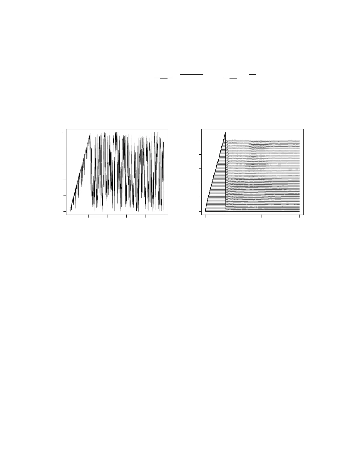
Split Sampling: Exp ectations, Normalisation and Rare Ev en ts John R. Birge, Changgee Chang, and Nic holas G. Polson Bo oth Sc ho ol of Business ∗ First Draft: August 2012 This Draft: Octob er 2013 Abstract In this pap er w e dev elop a metho dology that w e call split sampling metho ds to es- timate high dimensional exp ectations and rare even t probabilities. Split sampling uses an auxiliary v ariable MCMC sim ulation and expresses the exp ectation of in ter- est as an in tegrated set of rare ev ent probabilities. W e deriv e our estimator from a Rao-Blac kwellised estimate of a marginal auxiliary v ariable distribution. W e illus- trate our metho d with tw o applications. First, we compute a shortest netw ork path rare ev ent probabilit y and compare our method to estimation to a cross en trop y ap- proac h. Then, we compute a normalisation constant of a high dimensional mixture of Gaussians and compare our estimate to one based on nested sampling. W e discuss the relationship b et w een our metho d and other alternatives suc h as the pro duct of conditional probability estimator and imp ortance sampling. The metho ds developed here are a v ailable in the R pack age: SplitSampling . Keyw ords: Rare Even ts, Cross En tropy , Pro duct Estimator, Slice Sampling, MCMC, Imp ortance Sampling, Serial T emp ering, Annealing, Adaptiv e MCMC, W ang-Landau, Nested Sampling, Bridge and Path Sampling. ∗ E-mail: john.birge@c hicagob o oth.edu, c hanggee@uc hicago.edu, ngp@c hicagob o oth.edu. W e w ould lik e to thank the participants at the conference in honor of Pietrio Muliere at Bo cconi, September 13-15, 2012 for their helpful commen ts. The authors’ work w as supported b y the Univ ersity of Chicago Booth Sc ho ol of Business. 1 1 In tro duction In this pap er we dev elop a metho dology we refer to as split sampling metho ds to provide more precise estimates for high dimensional exp ectations and rare even t probabilities. W e sho w that more precise estimators can b e ac hieved by splitting the exp ectation of in terest in to a n umber of easier-to-estimate normalisation constan ts and then integrating those es- timates to pro duce an estimate of the full exp ectation. T o do this, w e emplo y an auxiliary v ariable MCMC approac h with a family of splitting functions and a w eighting function on the conditional distribution of the auxiliary random v ariable. W e allow for an adaptive MCMC approach to sp ecify our w eighting function. W e relate our metho d to the pro duct estimator (Diaconis and Holmes, 1994, Fishman, 1994) which splits the rare even t prob- abilit y in to a set of relatively larger conditional probabilities which are easier to estimate and to nested sampling (Skilling, 2006) for the estimation of exp ectations. Other v ari- ance reduction tec hniques, suc h as con trol v ariates will provide further efficiency gains (see Dellap ortas and Kon to yiannis, 2012, Mira et al, 2012). There are t wo related approaches in the literature. One approac h is for estimating exp ectations is nested sampling (Skilling, 2006) whic h sequen tially estimates the quan tiles of the lik eliho o d function under the prior. Other normalisation metho ds include bridge and path sampling (Meng and W ong, 1996, Gelman and Meng, 1998), generalized v ersions of the W ang-Landau algorithm (W ang and Landau, 2001), and the TP A algorithm of Hub er and Sc hott (2010). Serial temp ering (Gey er, 2010) and link ed imp ortance sampling (Neal, 2005) pro vide ratios of normalisation constan ts for a discrete set of unnormalised densities. The second approac h is cross entrop y (Rubinstein and Glynn, 2009, Asm ussen et al, 2012) whic h sequen tially constructs an optimal v ariance-reducing imp ortance function for calculating rare ev en t probabilities. W e show that our adaptiv ely c hosen w eigh ted MCMC algorithm can provide efficiency gains o v er cross entrop y methods. The problem of interest is to calculate an expectation of in terest, Z = E π ( L ( x )), where L is a lik eliho o d and π is a prior measure. F or rare ev ent probabilities, Z ( m ) = E π ( L m ( x )), and the splitting functions L m ( x ) are sp ecified b y lev el sets in the likelihoo d, namely L m ( x ) = I ( L ( x ) > m ). This o ccurs naturally in the rare even t simulation literature and in nested sampling. T o dev elop an efficient estimator, we define a join t split sampling split distribution, π S S ( x , m ), on x and an auxiliary v ariable m that tilts the conditional distribution with a weigh ting function, ω ( m ). W e pro vide a default setting for the weigh t function to matc h the sampling properties of the pro duct estimator and of nested sampling. 2 W e also allo w for the p ossibilit y of adaptiv ely learning a w eight function from the MCMC output. As with other ergo dic Mon te Carlo metho ds, we assume that the researc her can construct a fast MCMC algorithm for sampling our join t distribution. The rest of the pap er is outlined as follo ws. Section 2 details our split sampling method- ology . A key iden tit y “splits” the exp ectation of in terest in to an in tegrated set of rare ev en t normalisation constan ts. MCMC then pro vides an estimator of the marginal distribution of the auxiliary v ariable, whic h in turn pro vides our ov erall estimator. W e pro vide a num b er of guidelines for sp ecifying our w eight function in b oth discrete and contin uous settings. Section 3 describ es the relationship with the pro duct estimator and nested sampling meth- o ds. In both cases, w e provide a theorem that pro vides a default choice of w eight function to matc h the sampling b ehavior of the product estimator and nested sampling. Section 4 applies our metho dology to a shortest path rare ev ent probabilit y and to the calculation of a normalisation constant for a spik e-and-slab mixture of Gaussians. W e illustrate the efficiency gains of split sampling ov er crude Mon te Carlo, the pro duct estimator and the cross entrop y method. Finally , Section 5 concludes with directions for future research. 2 Split Sampling W e no w in tro duce the notation to characterize the estimation problems and to develop our metho d. The cen tral problem is to calculate an exp ectation of a non-negative functional of interest, whic h we denote as L ( x ), under a k -dimensional probability distribution π ( x ). W e write this exp ectation as: Z = E π ( L ( x )) = Z X L ( x ) π ( x ) d x . The corresp onding rare ev ent probabilit y is giv en b y Z ( m ) = E π ( L m ( x )) = P ( L ( x ) > m ) W e interpret π ( x ) as a “prior” distribution, L ( x ) as a lik eliho o d, and m as an auxiliary v ariable. Given a family of splitting functions, L m ( x ), their normalisation constants are, Z ( m ) = R X L m ( x ) π ( x ) d x . F or rare ev en ts, L m ( x ) = I ( L ( x ) > m ) where m is large. Here w e assume that L ( x ) is con tinuous with respect to the prior π and Z (0) = P ( L ( x ) > 0) = 1. 3 Split sampling works as follows. W e define the set of “tilted” distributions and corre- sp onding normalisation constan ts b y π ( x | m ) = L m ( x ) π ( x ) Z ( m ) where Z ( m ) = Z X L m ( x ) π ( x ) d x . F or rare ev en ts, L m ( x ) = I ( L ( x ) > m ) and π ( x | m ) ∼ π ( x | L ( x ) > m ) corresponds to conditioning on lev el sets of L ( x ). The Z ( m )’s corresp ond to “rare” even t probabilities Z ( m ) = Z X L m ( x ) π ( x ) d x = Z L ( x ) >m π ( x ) d x = P π ( L ( x ) > m ) . F or the functional L ( x ), the exp ectation of interest, Z , is an in tegration of the rare even t probabilities. Using F ubini and writing L ( x ) = R L ( x ) 0 dm we hav e the k ey iden tity Z = Z X L ( x ) π ( x ) d x = Z X  Z L ( x ) >m π ( x ) dm  d x = Z ∞ 0 Z ( m ) dm . W e hav e “split” the computation of Z in to a set of easier to compute normalisation con- stan ts Z ( m ). W e will sim ultaneously provide an estimator b Z ( m ) and b Z = R ∞ 0 b Z ( m ) dm . T o do this, we further introduce a weigh t function on the auxiliary v ariable, ω ( m ), and the cumulativ e weigh t Ω( m ) = R m 0 ω ( s ) ds . The joint split sampling density , π S S ( x , m ), is defined with π S S ( x | m ) ≡ π ( x | m ) as π S S ( x , m ) = π S S ( x | m ) · ω ( m ) Z ( m ) Z W , where Z W = R ∞ 0 ω ( s ) Z ( s ) ds . The marginals on m and x are π S S ( m ) = ω ( m ) Z ( m ) Z W and π S S ( x ) = Ω( L ( x )) π ( x ) Z W (1) where Ω( L ( x )) = R L ( x ) 0 ω ( s ) ds . The key feature of our split sampling MCMC dra ws, ( x , m ) ( i ) ∼ π S S ( x , m ), are that they provide an efficien t Rao-Blac kwellised estimate of the marginal b π S S ( m ) without the kno wledge of the Z ( m )’s. W e no w sho w how to estimate b Z ( m ) and b Z = R ∞ 0 b Z ( m ) dm . With L m ( x ) = I ( L ( x ) > m ), the joint splitting densit y is π ( x , m ) = π ( m ) π ( x | M = m ) = ω ( m ) Z ( m ) Z W I ( L ( x ) > m ) π ( x ) Z ( m ) 0 < m < ∞ . 4 The conditional p osterior of the auxiliary index m giv en x is π ( m | x ) = ω ( m ) I ( m < L ( x )) / Ω( L ( x )) where Ω( m ) = Z m 0 ω ( s ) ds The densit y is prop ortional to the w eigh t function ω ( m ) on the interv al [0 , L ( x )]. Slice sampling corresponds to ω ( m ) ≡ 1 and uniform sampling on [0 , L ( x )]. This w ould lead to direct dra ws from the posterior distribution L ( x ) π ( x ) / Z and the resultant estimator w ould b e the Harmonic mean. Our approac h will weigh t tow ards regions of smaller m v alues to pro vide an efficient estimator of all the rare even t probabilities Z ( m ) and hence of Z . The marginal densit y estimator of m is b π S S ( m ) = 1 N N X i =1 π ( m | x ( i ) ) = 1 N N X i =1 ω ( m ) I { L ( x ( i ) ) > m } Ω( L ( x ( i ) )) , 0 < m < ∞ = φ N ( m ) ω ( m ) where φ N ( m ) = 1 N N X i =1 I { m < L ( x ( i ) ) } Ω( L ( x ( i ) )) . This is a re-w eighted version of the initial weigh ts ω ( m ). The function φ N ( m ) will b e used to adaptively re-balance the initial w eigh ts ω ( m ) in our adaptiv e v ersion of the algorithm, see Section 4. W e now deriv e estimators for Z ( m ) and Z by exploiting a Rao-Blackw ellised estimator for the marginal density , π S S ( m ). F rom (1), w e ha ve π S S ( m ) ∝ ω ( m ) Z ( m ) and so an estimate of Z ( m ) is giv en b y b Z ( m ) Z (0) = ω ( m ) − 1 b π S S ( m ) ω (0) − 1 b π S S (0) . With Z (0) = 1, this provides a new estimator b Z ( m ), where x ( i ) ∼ π S S ( x ), given by b Z ( m ) = φ N ( m ) φ N (0) = P i : L ( x ( i ) ) >m Ω( L ( x ( i ) )) − 1 P N i =1 Ω( L ( x ( i ) )) − 1 . T o find b Z = R ∞ 0 b Z ( m ) dm , we use the summation-in tegral counterpart to F ubini and the fact that L ( x ( i ) ) = R L ( x ( i ) ) 0 dm to yield Z ∞ 0 X i : L ( x ( i ) ) >m Ω( L ( x ( i ) )) − 1 dm = N X i =1 Ω  L ( x ( i ) )  − 1 L ( x ( i ) ) . 5 Therefore, we hav e our estimator b Z = N X i =1 Ω  L ( x ( i ) )  − 1 P N i =1 Ω( L ( x ( i ) )) − 1 L ( x ( i ) ) . W e no w describ e our split sampling algorithm. Algorithm: Split Sampling • Dra w samples ( x , m ) ( i ) ∼ π S S ( x , m ) by iterating π S S ( x | m ) and π S S ( m | x ) • Estimate the marginal distribution, b π S S ( m ), via b π S S ( m ) = 1 N N X i =1 ω ( m ) L m ( x ( i ) ) R M 0 ω ( m ) L m ( x ( i ) ) dm . • Estimate the individual normalisation constan ts, b Z ( m ), via b Z ( m ) = P i : L ( x ( i ) ) >m Ω( L ( x ( i ) )) − 1 P N i =1 Ω( L ( x ( i ) )) − 1 . (2) • Compute a new estimate, b Z , via b Z = N X i =1 Ω  L ( x ( i ) )  − 1 P N i =1 Ω( L ( x ( i ) )) − 1 L ( x ( i ) ) . (3) A practical use of the algorithm will in volv e a discrete grid 0 = m 0 < m 1 < · · · < m T . W e write the rare even t probabilities Z t ≡ Z ( m t ) and the weigh ts ω ( m ) = P T t =0 ω t δ m t ( m ). The marginal probabilities π t ≡ π ( m t ) are estimated by Rao-Blac kw ellization as b π t = 1 N N X i =1 π ( m t | x ( i ) ) = 1 N N X i =1 ω t I { L ( x ( i ) ) >m t } P T s =0 ω s I { L ( x ( i ) ) >m s } , 0 ≤ t ≤ T . With Z 0 = 1, the estimator is b Z t = ω 0 b π t /ω t b π 0 for 0 ≤ t ≤ T . In the next sections w e provide a default c hoice of weigh ts to match the sampling b eha viour of the pro duct estimator and nested sampling together with an adaptiv e MCMC scheme for estimating the weigh ts. First, we turn to con vergence issues. 6 2.1 Con v ergence and Mon te Carlo standard errors Rob erts and Rosen thal (1997), Mira and Tierney (2002) and Hob ert et al (2002) who pro vide general conditions for geometric ergo dicity of slice sampling. Geometric ergo dicity will imply a Mon te Carlo CL T for calculating asymptotic distributions and standard errors. Our c hain is geometrically ergo dic if π S S is b ounded, and there exists an α > 1 such that G ( m ) is nonincreasing on (0 ,  ) for some  > 0 where G ( m ) = m α − 1 +1 ∂ Z ( m ) /∂ m . Then we can apply a cen tral limit theorem to ergo dic a v erages of the functional g ( x , m ) = Ω( L ( x )) − 1 I ( L ( x ) > m ) whic h yields the condition Z Θ g ( x , m ) 2+  π S S ( x ) d x = Z L ( x ) ≥ m Ω ( L ( x )) − (1+  ) π ( d x ) < ∞ W e ha ve a cen tral limit theorem for b Z ( m ) / Z W at any u , where 0 < σ 2 Z ( m ) < ∞ √ N Z W n b Z ( m ) − Z ( m ) o D ⇒ N  0 , σ 2 Z ( m )  This argument also w orks at m = 0 as long as σ 2 Z (0) < ∞ . 2.2 Imp ortance Sampling The standard Monte Carlo estimate of Z = E π ( L ( x )) is b Z = (1 / N ) P N i =1 L ( x ( i ) ) where x ( i ) ∼ π ( x ), with dra ws possibly obtained via MCMC. This is to o inaccurate for rare even t probabilities. V on Neumann’s original view of importance sampling was as a v ariance reduction to improv e this estimator. By viewing the calculation of an exp ectation as a problem of normalising a p osterior distribution, w e can write π L ( x ) = L ( x ) π ( x ) / Z where Z = Z X L ( x ) π ( x ) d x . Imp ortance sampling uses a blank et g ( x ) to compute Z = Z X L ( x ) π ( x ) g ( x ) g ( x ) d x ≈ b Z I S = 1 N N X i =1 L ( x ( i ) ) π ( x ( i ) ) g ( x ( i ) ) where x ( i ) ∼ g ( x ) . 7 Pic king g ( x ) to b e the p osterior distribution L ( x ) π ( x ) / Z leads to the estimator b Z I S = Z with zero v ariance. While impractical, this suggests finding a class of imp ortance blank ets g ( x ) that are adaptiv e and dep end on L ( x ) can exhibit goo d Monte Carlo properties. Split sampling sp ecifies a class of imp ortance sampling blank ets, indexed by ω ( m ), by g ω ( x ) = n R L ( x ) 0 ω ( s ) ds o π ( x ) Z W = Ω( L ( x )) π ( x ) Z W . The estimator b Z ( m ) in (2) can b e viewed as an importance sampling estimator where we a verage Ω  L ( x ( i ) )  − 1 o ver the splitting set L ( x ( i ) ) > m with x ( i ) ∼ π S S ( x ). Similarly w e can express b Z as an imp ortance sampling estimator as in (3) which uses a prop osal distribution prop ortional to Ω( L ( x )) π ( x ). 3 Comparison with the Pro duct Estimator and Nested Sampling 3.1 Pro duct Estimator A standard approac h to calculating the rare ev ent probability Z ( m ) = P ( L ( x ) > m ) is the pro duct estimator. W e set m = m T for some T > 0 and introduce a discrete grid m t of m -v alues starting at m 0 = 0. The conditional probabilit y estimator writes Z ( m ) = Z T = T Y t =1 P ( L ( x ) > m t | L ( x ) > m t − 1 ) = T Y t =1 P ( L ( x ) > m t ) P ( L ( x ) > m t − 1 ) or equiv alently Z ( m ) = Z T = Q T t =1 Z t / Z t − 1 . V ariance reduction is ac hieved by splitting Z T in to pieces Z t / Z t − 1 of larger magnitude whic h are relatively easier to estimate. With x ( i ) t ∼ π t − 1 ( x ) ≡ π ( x | L ( x ) > m t − 1 ), w e estimate Z t Z t − 1 = Z X L m t ( x ) π t − 1 ( x ) d x with d Z t Z t − 1 = 1 N N X i =1 L m t ( x ( i ) t ) . Giv en N indep endent samples from the tilted distributions π t − 1 ( x ) for eac h t , we ha v e b Z T = T Y t =1 1 N N X i =1 L m t ( x ( i ) t ) and V ar  b Z T  Z 2 T = T Y t =1  σ 2 t µ 2 t + 1  − 1 8 with mean µ t = E ( \ Z t / Z t − 1 ) and v ariance σ 2 t = V ar( \ Z t / Z t − 1 ). The pro duct estimator, as well as the cross-entrop y estimator, relies on a set of indep endent samples dra wn in a sequen tial fashion. Split sampling, on the other hand, uses a fast MCMC and ergo dic a veraging to provide an estimate b Z T . The Mon te Carlo v ariation V ar( b π S S ( m ) / b π S S (0)) can b e determined from the output of the chain. Con trolling the Monte Carlo error of this estimator is straigh tforward due to indep endent samples with relativ e mean squared error, see Fishman (1994) and Garv els et al (2002), 3.1.1 Matc hing the Pro duct Estimator Sampling Distribution W e can now compare the pro duct estimator with split sampling. Supp ose 0 < ρ < 1 and let m t b e the grid p oints of L ( x ) for 0 ≤ t ≤ T where x ∼ π ( x ). By construction, m t are the tail ρ t -quan tile of L ( x ), and we ha v e Z t = ρ t . There are tw o v ersions of the pro duct estimator. First, the standard pro duct estimator has the long-run sampling distribution π P E ( x ) = 1 T T X t =1 π t − 1 ( x ) = 1 T T X t =1 π ( x ) I ( L ( x ) > m t − 1 ) Z t − 1 . The second pro duct estimator includes samples from the previous lev el generation that w ere ab o v e the threshold. This has the long-run sampling distribution π P E I ( x ) ∝ π ( x ) + T X t =2 Z t − 2 − Z t − 1 Z t − 2 π t − 1 ( x ) = π ( x ) + T X t =2 Z t − 2 − Z t − 1 Z t − 2 Z t − 1 π ( x ) I ( L ( x ) > m t − 1 ) . W e call this the pro duct estimator with inclusion. Theorem 1 (Pro duct Estimator) The two pr o duct estimators and the split sampling ar e r elate d as fol lows. The standar d pr o duct estimator c orr esp onds to the (discr ete) split sampling with ω t = 1 / Z t . The pr o duct estimator with inclusion is e quivalent to split sam- pling with cumulative weights Ω t = t X i =0 ω i = 1 / Z t . 9 Split sampling with discrete knots m t , w eights ω t and Ω t = P t i =0 ω i has sampling distribution π S S ( x ) ∝ T X t =1 ω t − 1 π ( x ) I ( L ( x ) > m t − 1 ) ∝ T − 1 X t =1 Ω t − 1 π ( x ) I ( m t − 1 < L ( x ) < m t ) + Ω T − 1 π ( x ) I ( L ( x ) ≥ m T − 1 ) . Therefore, this is equiv alen t to the pro duct estimator if and only if, for 0 ≤ t < T , ω t = 1 Z t , and Ω t = t X i =1 1 Z i . As m t are the tail ρ t -quan tile of L ( x ), w e ha ve ω t = ρ − t and Ω t = ρ ( ρ − t − 1) 1 − ρ . F or the pro duct estimator with inclusion, the equiv alen t split sampling weigh ts are Ω t = 1 + t X i =1 Z i − 1 − Z i Z i − 1 Z i = 1 Z t = ρ − t . 3.2 Nested Sampling W e now provide a comparison with nested sampling. W e provide a sp ecification of ω ( m ) so that the sampling distribution of matches that of nested sampling. W e can adaptiv ely determine the v alues from our MCMC output. Let Q L ( q ) b e the q -quantile of the lik eliho o d function L ( x ) under the prior π ( x ). Then, nested sampling expresses Z = Z 1 0 Q L ( q ) dq = Z ∞ 0 Q L (1 − e − Y ) e − Y d Y . where q = 1 − e − Y . This in tegral can b e appro ximated b y quadrature Z ≈ ∞ X i =1 ( e − i − 1 N − e − i N ) Q L (1 − e − i N ) . The larger N is, the more accurate the approximation, and so this suggests the following estimator b Z = n − N X i =1 ( e − i − 1 N − e − i N ) L i + e − n − N N N N X i =1 L n − N + i , 10 where L i are the sim ulated (1 − e − i N )-quan tiles of likelihoo ds with resp ect to the prior. Here, n is the total n umber of samples. Nested Sampling is a sequen tial sim ulation procedure for finding the  1 −  N N +1  i  -quan tiles, L i , by sampling π ( x | L ( x ) > L i − 1 ). Brew er et al (2011) prop ose a diffuse nested sampling approac h to determine the levels L t . Both nested and diffuse nested sampling are product estimator approaches. The quan tiles 0 = L 0 < . . . < L t < . . . are c hosen so that eac h lev el L t o ccupies ρ = e − 1 times as muc h prior mass as the previous level L t − 1 . Diffuse nested sampling ac hieves this b y sequentially sampling from a mixture imp ortance sampler P t − 1 j =1 w j I ( L ( x ) > L j − 1 ) π ( x ) where the weigh ts are exp onen tial w j ∝ e κ ( j − t ) for some κ . MCMC metho ds are used to tra verse this mixture distribution with a random walk step for the index j that steps up or down a level with equal probability . A new level is added using the (1 − e − 1 )-quan tile of the likelihoo d dra ws. Using diffuse nested sampling allo ws some chance of the samples’ escaping to lo w ered constrained lev els and to explore the space more freely . One cav eat is that a large con tribution can come from v alues of x ( z ) near the origin and we hav e to find man y lev els T to obtain an accurate appro ximation. Murra y et al (2006) pro vide single and m ultiple sample v ersions of nested sampling algorithms. If L max = sup x L ( x ) is kno wn, w e sample as follo ws: 1. Set X = 1 , Z = 0 , i = 1. 2. Generate N samples x ( i ) from π ( x ) and sort L i = L ( x ( i ) ). 3. Rep eat while L max X > Z : (a) Set Z = Z + L i X/ N and X = (1 − 1 / N ) X . (b) Generate x ( i + N ) ∼ π ( x ) I ( L ( x ) > L i ) and set L i + N = L ( x ( i + N ) ). (c) Sort L i ’s and set i = i + 1. 4. Set Z = Z + ( X/ N ) P N j =1 L i + j − 1 and stop. If L max is not kno wn, replace step 3 with: 3(a). Rep eat while L i + N − 1 X > Z : 11 3.2.1 Matc hing the Nested Sampling Distribution W e no w c ho ose ω ( m ) to match the sampling properties of nested sampling. The main difference b et w een split and nested sampling is that in split sampling w e sp ecify a w eight function ω ( m ) for 0 < m < ∞ and sample from the full mixture distribution, rather than employing a sequential approac h for grid selection whic h requires a termination rule. Another difference is that split sampling estimator does not need to kno w the ordered L i ’s. W e can no w matc h the sampling distributions of split and nested sampling (see, Skilling, 2006). The exp ected num b er of samples L i less than m is − N log Z ( m ). Assume N = 1 for a while. Since Z ( L i ) / Z ( L i − 1 ) are indep enden t standard uniforms and − log Z ( L k ) = − k X i =1 log Z ( L i ) Z ( L i − 1 ) for k ≥ 1 , the distribution of the n umber of samples L i less than m is same as the n um b er of arriv als b efore − log Z ( m ) of a P oisson pro cess with rate 1. F or general N , it only c hanges the arriv al rate of the Poisson pro cess in to N . Theorem 2 (Nested Sampling) If we pick the weights ω ( m ) such that Ω( m ) = 1 / Z ( m ) Then the sampling distributions of split and neste d sampling match. The sampling distribution of the nested sampling for finite n is hard to calculate, but w e can observe limiting results. As n → ∞ , if N/n → λ , then w e ha v e Z N S ( m ) = P N S ( L ( x ) > m ) = 1 + lim n,N →∞ N n log Z ( m ) = 1 + λ log Z ( m ) . Split sampling has marginal densit y of x giv en b y π S S ( x ) = Ω( L ( x )) π ( x ) Z W with Ω( m ) = Z m 0 ω ( s ) ds . The tail distribution function Z S S ( m ) = π S S ( L ( x ) > m ) is then Z S S ( m ) = Z ∞ 0 Z X I { L ( x ) >m } ω ( s ) Z ( s ) Z W I { L ( x ) >s } π ( x ) Z ( s ) d x ds = R ∞ 0 ω ( s ) Z ( m ∨ s ) ds Z W = Z ( m )Ω( m ) + R ∞ m ω ( s ) Z ( s ) ds Z W . 12 W e now find the imp ortance splitting density that matc hes the nested sampling distribu- tional prop erties in the sense that Z N S ( m ) = Z S S ( m ). Since Z 0 N S ( m ) = λZ 0 ( m ) Z ( m ) and Z 0 S S ( m ) = Z 0 ( m )Ω( m ) Z W , where Z 0 N S ( m ) = ∂ Z N S ( m ) /∂ m . W e therefore set Ω( m ) = 1 / Z ( m ). Since Z ( m ) is unknown, w e are not ready to b egin sampling. As a remedy we prop ose appro ximating Z ( m ). W e estimate Z t ’s for certain grid p oin ts { m t } 0 ≤ t M ( i − 1) ), and set L i = L ( x ( i ) ). (b) Obtain M ( i ) = Ω − 1 ( U i ) if U i > 1 or M ( i ) = 0 otherwise, where U i ∼ Unif (0 , Ω( L i )). (c) Rep eat (a) and (b) until w e ha ve N lev el visits to lev el T − 1. (d) Cho ose the (1 − ρ )-quantile of likelihoo ds of lev el T − 1 as m T . (e) Set b Z T = ρ − T and Ω T = b Z − 1 T . Under the condition Ω( m ) = Z ( m ) − 1 , the c hain will visit each lev el roughly uniformly . Ho wev er, it ma y take a long time to reach the top level, and the uncertaint y in Ω may act lik e a hurdle for visiting upp er levels. With these concerns, it is desirable to fav or upp er lev els b y replacing step (d) with (d1) Set Ω T = e Λ T b Z − 1 T . W e call Λ the b o osting factor as Λ increases the preference for the upp er lev els. This reduces the search time and ensures the time complexity to b e O ( T ). T o further exp edite this pro cedure, we may put more weigh t on the top level T b y substituting (d) with the step: 13 (d2) Set Ω T − 1 = e Λ( T − 1) b Z − 1 T − 1 and Ω T = β e Λ T − 1 e Λ − 1 b Z − 1 T . F or example, if β = 1, the chain sp ends half of the time on the top level and the other half bac ktracking the other lev els. Once we identify all levels, our split sampling algorithm runs: 1. Set i = 0 and ν t = ν init b Z t for each t = 0 , 1 , . . . , T . 2. While i ≤ n , set i = i + 1. (a) Dra w ( x , M ) ( i ) ∼ π S S ( x , m ) with { m t } 0 ≤ t m } Ω( L ( x ( i ) )) ) ω ( m ) . The densit y estimate will b e zero for m > max i L  x ( i )  b y construction. W e also hav e a set of estimates b Z ( m ) = P i : L ( x ( i ) ) >m Ω( L ( x ( i ) )) − 1 / P N i =1 Ω( L ( x ( i ) )) − 1 where x ( i ) ∼ π S S ( x ) whic h can b e used to re-balance to weigh ts Ω( m ) = Z ( m ) − 1 . Giv en an initial run of the algorithm, w e can re-prop ortion the prior w eight function to regions we ha ve not visited frequently enough. T o accomplish this, let φ ( m ) b e a desired target distribution for π S S ( m ), for example a uniform measure. Then re-balance the w eights in versely prop ortional to the visitation probabilities and set the new w eigh ts ω ? ( m ) by ω ? ( m ) ω ( m ) = ω ( m ) µ N ( m ) = I { L ( x ( i ) ) > m } Ω( L ( x ( i ) )) . This will only adjust our w eights in the region where m < max i L ( x ( i ) ). As the algorithm pro ceeds we will sample regions of higher lik eliho o d v alues and further adaptive our weigh t function. Other c hoices for weigh ts are a v ailable. F or example, in man y normalisation problems Z ( m ) will b e exp onential in m due to a Laplace approximation argumen t. This suggests taking an exp onen tial w eighting ω ( m ) = κe κm for some κ > 0. In this case, w e hav e Ω( m ) = Z m ∧ M 0 ω ( s ) ds = e κ ( m ∧ M ) − 1 . The marginal distribution is π S S ( x ) = ( e κ ( L ( x ) ∧ M ) − 1) π ( x ) R ∞ 0 κe κs Z ( s ) ds . W e can also sp ecify ω ( m ) to deal with the p ossibilit y that the c hain migh t not hav e visited all states b y setting a threshold ω max whic h corresp onds to the maxim um allo w able increase in the log-prior weigh ts. This leads to a re-balancing rule ω ? ( m ) ω ( m ) = min  max m µ N ( m ) µ N ( m ) , e ω max  , 15 where we hav e also re-normalised the v alue of the largest state to one. When L max is av ailable, we set M = L max and ω ( m ) = 0 for m > M . T o initialise ω ( m ), we use the harmonic mean b Z − 1 L max for ω ( M ) and an exp onen tial in terp olation for ω ( m ). Dra wing x ( i ) ∼ π M ( x ) = L ( x ) π ( x ) / Z , we hav e Z − 1 M = E π M  L − 1 M ( x )  to estimate b ω ( M ) = 1 N N X i =1 L − 1 M ( x ( i ) ) . The harmonic mean estimator (Raftery et al, 2007) is kno wn to hav e p o or Monte Carlo error v ariance prop erties (P olson, 2006, W olp ert and Schmidler, 2012) although we are estimating ω ( m ) and not its in v erse. W e can extend this insigh t to a fully adaptiv e update rule for ω N ( m ), similar to sto chas- tic appro ximation sc hemes. Define a sequence of decreasing p ositive step sizes γ n with P ∞ n =1 γ − 1 n = ∞ , P ∞ n =1 γ − 2 n < ∞ . A practical recommendation is γ n = C n − α where α ∈ [0 . 6 , 0 . 7], see e.g. Sato and Ishii (2000). Another approac h is to w ait until a “flat histogram” (FH) condition holds: max m ∈{ m t } µ N ( m ) − φ ( m ) < c . for a pre-sp ecified tolerance threshold, c . The measure µ N ( m ) = (1 / N ) P N i =1 #  m ( i ) = m  trac ks our curren t estimate of the marginal auxiliary v ariable distribution. The Rao- Blac kwellised estimate b π S S ( m ) further reduces v ariance. The empirical measure can b e used to up date ω N ( m ) as the c hain progresses. Let κ N denote the points at whic h γ κ N will b e decreased according to its schedule. Then an up date rule which guarantees con vergence is to set log ω κ N ( m ) ← log ω κ N − 1 ( m ) + γ κ N ( µ κ N ( m ) − φ ( m )) . Jacob and Ryder (2012) show that if γ N is only up dated on a sequence of v alues κ N whic h corresp ond to times that a “flat-histogram” criterion is satisfied, then conv ergence ensues and the FH criteria is ac hieved in finite time. After up dating ω κ N ( m ), we re-set the coun ting measure µ κ N ( m ) and contin ue. Other adaptive MCMC con v ergence metho ds are av ailable in Atc hade and Liu (2010), Liang et al (2007), and Zhou and W ong (2008). Bornn et al (2012) provides a parallelisable algorithm for further efficiency gains. Peskun (1973) pro vides theoretical results on optimal MCMC chains to minimise the v ariance of MCMC functionals. 16 One desirable Monte Carlo prop erty for an estimator is a b ounded co efficient of v ari- ation. F or simple functions, L ( x ) = x and max i x i , mixture imp ortance functions achiev e suc h a goal, see Iyengar (1991) and Adler et al (2008). Madras and Piccioni (1999, section 4) hin t at the efficiency prop erties of dynamically selected mixture imp ortance blankets. Gramacy et al (2010) prop ose the use of imp ortance temp ering. Johansen et al (2006) use logit annealing implemen ted via a sequen tial particle filtering algorithm. 4.1 Cho osing a Discrete Co oling Sc hedule W e suggest a simple, sequen tial, empirical approac h to selecting a “co oling schedule” in our approac h. Sp ecifically , set m 0 = 0, then given m t − 1 w e sample x ( i ) ∼ π m t − 1 ( x ) ∼ π ( x | L ( x ) > m t − 1 ). W e order the realisations of the criteria function L ( x ( i ) ) and set m t equal to the (1 − ρ )-quan tile of the L ( x ( i ) ) samples. This provides a sequential approac h to solving ρ = P ( L ( x ) > m t | L ( x ) > m t − 1 ) = P ( L ( x ) > m t ) / P ( L ( x ) > m t − 1 ) = Z t / Z t − 1 . A num b er of authors hav e proposed “optimal” choices of ρ , whic h implicitly defines a co oling schedule, m t , for 0 ≤ t ≤ T . L’Ecuy er et al (2006) and Amrein and Kunsc h (2011) prop ose ρ = e − 2 and 0 . 2, resp ectiv ely . Hub er and Schott (2010) define a well-balanced sc hedule as one that satisfies e − 1 < ρ < 2 e − 1 . They sho w that such a c hoice leads to fast algorithms. The difficult y is in finding the righ t order of magnitude of M and the asso ciated sc hedule m t that ensures that eac h slice Z t / Z t − 1 is not exponentially small. F or rare ev ents, w e sample un til m t +1 > M and then set m T = M . Our initial estimate b Z = ρ − T and our w eights are ω ( m ) = ρ m . In hard cases, suc h as the m ultimo dal mixture of Gaussians, the normalising con- stan ts Z ( m ) are not exp onen tial in m . In such cases w e initialize the w eigh ts by a piecewise exp onential obtained b y in terp olating any p oin t m ∈ ( m t − 1 , m t ) by Ω( m ) = Ω t − 1 exp( κ t ( m − m t − 1 )) where κ t = log(Ω t / Ω t − 1 ) / ( m t − m t − 1 ). F or m > m T , we use Ω( m ) = Ω T . The final estimator is given b y b Z = Z ∞ 0 b Z ( m ) dm = T X t =1 Z m t m t − 1 b Z t − 1 exp( − κ t ( m − m t − 1 )) dm = T X t =1 ( b Z t − b Z t − 1 )( m t − m t − 1 ) log b Z t − log b Z t − 1 . Finally , our metho dology can b e view ed as an adaptive mixture imp ortance sampler. As w e rebalanced the weigh ts w e are adaptive c hanging the target distribution of our MCMC 17 algorithm rather than the traditional adaptive prop osal approaches with a fixed target. Other similar approac hes include Um brella sampling (T orrie and V alleau, 1997) whic h can b e seen as a precursor to many of the curren t adv anced MC strategies suc h as the W ang-Landau algorithm and its generalisations for sampling high dimensional m ultimo dal distributions. These algorithms exploit an auxiliary v ariable and by their adaptive nature impro ve estimates con tin uously as the sim ulation adv ances. The main difference is ho w eac h algorithm tra verses low and high energy states. The W ang-Landau algorithm aims to ac hiev e a uniform distribution on the auxiliary v ariable, thus sp ending more time in lo w energy states than high states states as opp osed to m ulticanonical sampling (Berg and Neuhaus, 1992), 1 /k -ensemble sampling (Hesselb o and Stinc hcombe, 1995) or sim ulated temp ering (Gey er and Thompson, 1995). 5 Applications 5.1 Rare Ev en t Shortest P ath Calculating rare ev ent probabilities is a common goal of man y problems. Rubinstein and Kro ese (2004) consider the total length of the shortest path on a w eigh ted graph with random w eights x = ( x 1 , . . . , x 5 ). Supp ose there are 4 vertices a , b , c , and d . The adjacen t w eight matrix is giv en by      0 x 1 x 2 ∞ x 1 0 x 3 x 4 x 2 x 3 0 x 5 ∞ x 4 x 5 0      . Eac h w eigh t x j follo ws an indep enden t exp onential distribution with scale parameter u j with joint distribution giv en b y π ( x | u ) = 5 Y j =1 1 u j ! exp − 5 X j =1 x j u j ! where u = (0 . 25 , 0 . 4 , 0 . 1 , 0 . 3 , 0 . 2) . The goal is to estimate the probabilit y of the rare even t corresp onding to the length of the shortest path from a to d Z ( γ ) = P ( S ( x ) > γ ) where S ( x ) = min( x 1 + x 4 , x 1 + x 3 + x 5 , x 2 + x 3 + x 4 , x 2 + x 5 ) . 18 W e will consider three cases: γ = 2 , 3 , and 4 where the true rare ev ent probabilities are Z (2) = 1 . 34 × 10 − 5 , Z (3) = 2 . 06 × 10 − 8 , and Z (4) = 3 . 10 × 10 − 11 . These can b e estimated b y the split sampler (SS) with L ( x ) = S ( x ) and lev el breakp oin ts { 0 = m 0 , m 1 , . . . , m T = γ } . b Z T ≡ b Z ( m T ) is the estimator. W e implement three other competing estimators. First, the crude Mon te Carlo (CMC) estimator simulates x ( i ) ∼ π ( x | u ) and estimates the rare ev ent probabilities by b Z ( γ ) = 1 N N X i =1 I { S ( x ( i ) ) >γ } . Second, the conditional probabilit y pro duct (CPP) estimator b Z ( γ ) calculates the (1 − ρ )- quan tile m t +1 of N 0 samples of S ( x ( t,i ) ) under x ( t,i ) ∼ π t ( x ) ∝ I { S ( x ) >m t } π ( x ) for all t = 0 , . . . , T − 1 with m 0 = 0, m T − 1 < γ , and m T ≥ γ . This estimator is defined as: b Z ( γ ) = T − 1 Y t =1 d Z t Z t − 1 ! d Z ( γ ) Z T − 1 = ρ T − 1 1 N 0 N 0 X i =1 I { S ( x ( T − 1 ,i ) ) >γ } . T o find x ( t,i ) w e need to sample π ( x | S ( x ) > m t ). W e use Gibbs sampling with complete conditionals π ( x i | x ( − i ) , S ( x ) > m ) given b y truncated exp onen tial distributions. By the lac k of memory prop ert y , w e ha ve π ( x 1 | x ( − 1) , S ( x ) > m ) = max(0 , m − x 4 , m − x 3 − x 5 ) + x ? 1 where x ? 1 ∼ E xp ( u 1 ) . The other conditionals π ( x i | x ( − i ) , S ( x ) > m ) follo w in a similar manner. Third, the cr oss-entr opy (CE) estimator (de Bo er et al, 2005) calculates an “optimal” imp ortance blank et, π ( x | b v T ), parameterised by b v T . Then it dra ws N 1 samples of x ( i ) ∼ π ( x | b v T ) and estimates the shortest path probabilit y b Z ( γ ) = 1 N 1 N 1 X i =1 I { S ( x ( i ) ) >γ } w ( x ( i ) ; u , b v T ) , where w ( x ( i ) ; u , b v T ) = π ( x ( i ) | u ) π ( x ( i ) | b v T ) . The sequential algorithm for finding b v T is similar in spirit to the pro duct estimator ap- proac h: set b v 0 = u and t = 1. Cho ose ρ ; t ypically ρ = 0 . 1. Then p erform 1. Dra w N samples of x ( i ) ∼ π ( x | b v t − 1 ). Let b γ t b e the (1 − ρ ) quan tile of S ( x ( i ) ). If b γ t > γ , set b γ t = γ . 19 T able 1: Rare ev ent probabilities simulation γ = 2 γ = 3 γ = 4 N CMC CE CPP SS CE CPP SS CE CPP SS 10 5 0.807 0.040 0.044 0.055 0.066 0.076 0.091 0.113 0.098 0.133 10 6 0.275 0.011 0.015 0.015 0.017 0.025 0.026 0.028 0.033 0.036 10 7 0.086 0.003 0.004 0.005 0.005 0.007 0.007 0.008 0.009 0.011 2. Up date b v t − 1 via cross-entrop y minimisation; b v t = P N i =1 I { S ( x ( i ) ) > b γ t } w ( x ( i ) ; u , b v t − 1 ) x ( i ) P N i =1 I { S ( x ( i ) ) > b γ t } w ( x ( i ) ; u , b v t − 1 ) . 3. If b γ t = γ , set T = t and exit. Otherwise, set t = t + 1 and go to step 1. 0 200 400 600 800 1000 0 5 10 15 20 25 Level T raverse Obs/10000 Lev el 0 200 400 600 800 1000 0 5 10 15 20 25 Conver g ence of Omega Obs/10000 log(Omega) Figure 1: The trace plot of visits to lik eliho o d levels and c hanges of Ω t in rare ev en t probabilit y example with γ = 4 T able 1 pro vides the sim ulation results. Each scenario was run 100 times and r elative RMS of eac h estimator wa s recorded. The CMC estimator w as only recorded for γ = 2 as the other even ts are to o rare to even ha ve a single count. The total sample size, N , w as 10 5 , 10 6 , or 10 7 . The tuning parameters for CE were ρ = 0 . 1, N 0 = 1 , 000 for γ = 2 20 0 1 2 3 4 5 6 7 8 9 10 11 12 γ = 2 0 20 40 60 80 100 0 1 2 3 4 5 6 7 8 9 10 11 12 13 14 15 16 17 18 γ = 3 0 10 20 30 40 50 60 70 0 1 2 3 4 5 6 7 8 9 11 13 15 17 19 21 23 25 γ = 4 0 10 20 30 40 50 Figure 2: Histogram of visits to lev els in rare ev ent probabilit y example and N 0 = 10 , 000 for γ = 3 , 4, and N 1 = N − T N 0 . F or CPP , we used ρ = e − 1 and N 0 = N/T where T is the n umber of required steps. F or split sampling (SS), w e set ρ = e − 1 , N lev el = 10 , 000 and ν init = 10 , 000 and Λ = 0 . 1. One can see the cross-en trop y metho d outperforms the others. It is b ecause it finds an efficien t imp ortance sampling function and uses indep endent samples. How ever, note that the split sampling estimator is almost as efficient as others despite of the fact that it is an MCMC estimator. F urther gains from split sampling are exp ected in higher dimensional problems with m ultiple modes where finding b v t at each stage in CE can b e cum b ersome in general. 5.2 Normalisation of a Mixture of Gaussians As an illustration of the adv antages of using split sampling we consider a centered and de- cen tered mixture of Gaussians. W e follo w the nested and diffuse nested sampling literature (Skilling, 2008, Brew er et al, 2011) and supp ose that x = ( x 1 , . . . , x C ) where C = 20. The centered lik eliho o d is giv en b y the classic Gaussian “spik e-and-slab” of width 0 . 01 and “plateau” of width 0 . 1, namely L C ( x ) = 100 20 Y i =1 1 √ 2 π u e − x 2 i 2 u 2 + 20 Y i =1 1 √ 2 π v e − x 2 i 2 v 2 , 21 The prior π ( x ) is uniform on [ − 0 . 5 , 0 . 5] C . In the de-centered multimodal mixture w e take L DC ( x ) = 100 20 Y i =1 1 √ 2 π u e − ( x i − 0 . 031) 2 2 u 2 + 20 Y i =1 1 √ 2 π v e − x 2 i 2 v 2 . The goal is to calculate the so-called evidence, Z = R L ( x ) π ( x ) d x = 101. 0 200 400 600 800 1000 0 20 40 60 80 100 Obs/10000 Lev el 0 200 400 600 800 1000 0 20 40 60 80 100 Obs/10000 Omega Figure 3: The trace plot of visits to lik eliho o d levels and changes of Ω t in cen tered Gaussians case W e implemen ted the split sampling algorithm as describ ed in 3.2.1 and 4.1. The nested sampling is implemen ted via MCMC b ecause drawing from the conditional distribution directly is not p ossible for this example. In b oth metho ds, w e used a random w alk MH prop osal distribution giv en b y x ? j = x j + N (0 , σ 2 ) where the density of the step size f ( σ ) ∝ 1 /σ on [10 − 4 . 5 , 1] for random chosen index j . T able 2 and the b o xplot in Figure 4 compare the p erformance of the nested sampling and the split sampling metho ds. F or eac h run, log b Z w ere recorded and their ro ot mean squares are rep orted in T able 2. The num b er of runs for each case is 500. Ov erall, the nested sampling w orks sligh tly b etter for the cen tered case. There is no adv antage for split sampling in this case, but it is showing as go o d performance, to o. F or the de-centered case, the diffuse nested sampling is preferable to the nested sam- pling, b ecause when the likelihoo d is multimodal, one needs to b e able to bac ktrack the 22 ● ● ● ● ● ● ● NS1 NS2 NS3 NS4 SS 4 6 8 10 12 14 Centered ● ● NS1 NS2 NS3 NS4 DNS SS 0 2 4 6 8 Decentered Figure 4: NS vs DNS vs SS T able 2: SS vs NS, u = 0 . 01, v = 0 . 1, centered at origin, rms of log ( b Z ) with true v alue log( Z ) = 4 . 615. The n umber of MCMC steps is reported p er each NS step. Algorithm P arameters RMS NS1 300 particles, 333 MCMC steps 0 . 557 NS2 1000 particles, 100 MCMC steps 0 . 260 NS3 3000 particles, 33 MCMC steps 0 . 174 NS4 10000 particles, 10 MCMC steps 3 . 647 SS ρ = e − 1 , T max = 100, ν = 5000, Λ = 10 0 . 207 lo wer levels of lik eliho o d to trav erse another mo de. W e implemen ted the diffuse nested sampling for comparison as stated in their pap er (Brew er et al, 2011). As sho wn in T able 3 and the b oxplot in Figure 4, the split sampling significantly outp erforms others. It is largely due to the fact that the split sampling freely visits the t wo mo des of lik eliho o d function and fast conv ergence of Ω t ’s and b Z t ’s as one can see in the plots in Figure 5. 23 T able 3: SS vs (D)NS, u = 0 . 01, v = 0 . 1, the spik e centered at (0 . 031 , . . . , 0 . 031), rms of log( b Z ) with log ( Z ) = 4 . 615. The n umber of MCMC steps is p er each NS step. Diffuse nested sampling (DNS, Brewer et al, 2011). Algorithm P arameters RMS NS1 300 particles, 333 MCMC steps 2 . 467 NS2 1000 particles, 100 MCMC steps 2 . 338 NS3 3000 particles, 33 MCMC steps 2 . 519 NS4 10000 particles, 10 MCMC steps 2 . 620 DNS Diffuse Nested Sampling 0 . 763 SS ρ = e − 1 , T max = 100, ν = 5000, Λ = 10 0 . 591 0 200 400 600 800 1000 0 20 40 60 80 100 Obs/10000 Lev el 0 200 400 600 800 1000 0 20 40 60 80 100 Obs/10000 Omega Figure 5: The trace plot of visits to lik eliho o d lev els and changes of Ω t in de-centered Gaussians case 6 Discussion The adv antage of the class of split sampling densities is that the resultan t estimator of Z can be implemen ted via an auxiliary MCMC algorithm from a joint distribution π S S ( x , m ) indexed b y a random auxiliary v ariable m . Moreo ver, it allows an adaptiv e c hoice of ω N ( m ) 24 to reduce the Monte Carlo error of the resultan t estimator. Conv ergence results rely on adaptiv e MCMC literature. Rob erts (2010) observes that MCMC metho ds are likely to ac hieve the largest efficiency gains in rare ev en t probabilities (Glasserman et al, 1999, Glynn et al, 2010) and in counting problems where the resultan t chains can b e hard to sample exactly . Split sampling illustrates the adaptive imp ortance sampling nature of nested sampling and cross-en trop y methods. There is also a clear relationship with slice sampling (P olson, 1996, Neal, 2003) as one can view the sampling of the p osterior, π L ( x ), as the marginal from the augmented distribution π ( x , m ) = I ( L ( x ) > m ) π ( x ) / Z . The main difference is that split sampling runs a Mark ov c hain that tra verses the whole space defined b y ( x , m ) to find regions where ω ( m ) needs to b e refined. Both CE and NS metho ds using a sequential sampling pro cedure as in the CPP estimator to split the quantit y of in terest in to estimable pieces. F urther researc h is required to tailor the specification of the weigh t function ω ( m ) to the problem at hand. W e leav e op en the question of an optimal choice of L m ( x ). Here w e hav e fo cused on L m ( x ) = I ( L ( x ) > m ), how ever, using logit-type functions might led to faster con verging MCMC algorithms. The k ey to the efficiency of split sampling is b eing able to construct a rapidly mixing MCMC algorithm to sample the mixture distribution π S S ( x , m ). W e aim to rep ort on direct applications in Bay esian inference in future work. F or example, Murray et al (2006) shows that nested sampling p erforms w ell for Mark o v random fields mo dels and split sampling should ha ve similar prop erties. 7 References Adler, R.J., J. Blanchet and J. Liu (2008). Efficien t simulation for tail probabilities of Gaussian random fields. Pr o c e e dings of the Winter Simulation Confer enc e , 328-336. Amrein, M. and H. K¨ unsc h (2011). A v arian t of importance sampling for rare ev ent estima- tion: fixed n umber of successes. ACM T r ansactions on Mo deling and Computer Simulation , 21(2), Article 13. Asm ussen, S. and P . Dupuis, R. Rub enstein and H. W ang (2012). Importance Sampling for Rare Ev ents. Encyclop e dia of Op er ations R ese ar ch (eds Gass, S. and M. F u), Kluw er. A tchad ´ e,Y.F. and J.S. Liu (2010). The W ang-Landau algorithm in general state spaces: applications and con vergence analysis. Statistic a Sinic a , 20, 209-233. 25 Berg, B.A. and T. Neuhaus (1992). Multicanonical ensem ble: A new approac h to sim ulate first-order phase transitions. Physic al R eview L etters , 68, 9-12. Bornn, L., P .E. Jacob, P . Del Moral and A. Doucet (2012). An adaptive W ang-Landau algorithm for automatic density exploration. J. Computational and Gr aphic al Statistics . de Bo er, P .T., D.P . Kro ese and R.Y. Rub enstein (2005). A T utorial on the cross-entrop y metho d. A nnals of Op er ations R ese ar ch , 134, 19-67. Brew er, B.J, L.B. P´ arta y and G. Cs´ an yi (2011). Diffusiv e Nested Sampling. Statistics and Computing , 21(4), 649-656. Dellap ortas, P . and I. Kon toyiannis (2012). Con trol v ariates for estimation based on re- v ersible MCMC samplers. Journal of R oyal Statistic al So ciety, B , 74(1), 133-161. Diaconis, P . and S. Holmes (1994). Three examples of the MCMC metho d. Discr ete Pr ob ability and Algorithms , 43-56. Fishman, G. (1994). Marko v c hain sampling and the Pro duct Estimator. Op er ations R ese ar ch , 42(6), 1137-1145. Garv els, M.J.J., J.C.W. v an Ommeren and D.P . Kro ese (2002). On the importance function in splitting sim ulation. Eur op e an T r ansactions on T ele c ommunic ations , 13(4), 363-371. Gelman, A. and X. Meng (1998). Sim ulating normalizing constan ts: from importance sampling to bridge sampling to path sampling. Statistic al Scienc e , 13, 163-185. Gey er, C.J. and E.A. Thompson (1995). Annealing Marko v c hain Mon te Carlo with appli- cations to ancestral inference. Journal of Americ an Statistic al Asso ciation , 90, 909-920. Gey er, C.J (2012). Ba yes factors via Serial T emp ering. T e chnic al R ep ort , Univ ersity of W ashington. Glasserman, P ., P . Heidelb erger, P . Shahabuddin and T.Za jic (1999). Multi-Level Splitting for rare ev ent probabilities. Op er ations R ese ar ch , 47(4), 585-600. Glynn, P .W., A. Dolgin, R.Y. Rubinstein and R. V aisman (2010). Ho w to generate uniform samples on discrete sets using the splitting metho d. Pr ob. Eng. Info. Sci. , 24(3), 405-422. Gramacy , R., R. Sam worth and R. King (2010). Imp ortance T empering. Statistics and Computing , 20(1), 1-7. Hesselb o, B. and R.B. Stinchcom b e (1995). Mon te Carlo Sim ulation and global optimisa- tion without parameters. Phys. R ev. L ett. , 74, 2151-2155. 26 Hub er, M. and S. Schott (2010). Using TP A for Bay esian Inference. Bayesian Statistics, 9 , 257-282. Iy engar, S. (1991). Imp ortance Sampling for T ail Probabilities. T e chnic al R ep ort 440, Stanford Universit y . Jacob, P .E. and R.J. Ryder (2012). The W ang-Landau algorithm reaches the Flat His- togram criterion in finite time. Ann. Appl. Pr ob ab. . Johansen, A.M., P . Del Moral and A. Doucet (2006). Sequen tial Monte Carlo Samplers for Rare Even ts. Pr o c e e dings of the 6th International Workshop on R ar e Event Simulation , 256-267. L’Ecuy er, P ., V. Demers and B. T uffin (2006). Splitting for Rare even t simulation. Pr o- c e e dings of the 2006 Winter Simulation Confer enc e , 137-148. Liang, F. (2005). Generalized W ang-Landau algorithm for Mon te Carlo computation. Jour- nal of Americ an Statistic al Asso ciation , 100, 1311-1337. Liang, F., C. Liu and R.J. Carroll (2007). Sto chastic approximation in Mon te Carlo com- putation. Journal of Americ an Statistic al Asso ciation , 102, 305-320. Madras, N. and M. Piccioni (1999). Imp ortance Sampling for F amilies of Distributions. A nnals of Applie d Pr ob ability , 9(4), 1202-1225. Meng, X-L and W. W ong (1996). Sim ulating ratios of normalising constants via a simple iden tity: a theoretical exp osition. Statistia Sinic a , 6, 831-860. Mira, A., R. Solgi, and D. Imparato (2012). Zero V ariance MCMC for Ba y esian Estimators. Statistics and Computing , 23(5), 653-662. Murra y , I., D.J.C. MacKay , Z. Ghahramani and J. Skilling (2006). Nested sampling for the Potts mo dels. A dvanc es in NIPS , 947-954. Neal, R.M. (2003). Slice Sampling. Annals of Statistics , 31(3), 705-767. Neal, R.M. (2005). Estimating ratios of normalising constan ts using linked imp ortance sampling. T e chnic al R ep ort No. 0511, Univ ersit y of T oron to. P eskun, P .H. (1973). Optim um Mon te Carlo sampling using Mark ov Chains. Biometrika , 60(3), 607-612. P olson, N.G. (1996). Conv ergence of Mark ov Chain Mon te Carlo Algorithms. Bayesian Statistics, 5 , 297-321. 27 P olson, N.G. (2006). Commen t on: “Estimating the in tegrated lik eliho o d in posterior sim ulation using the harmonic mean equalit y”. Bayesian Statistics, 8 , 415-417. Raftery , A.E., M.A. Newton, J.M. Satagopan and P .N. Krivitsky (2007). Estimating the in tegrated lik eliho o d via p osterior sim ulation using the Harmonic mean equality . Bayesian Statistics, 8 , 371-417. Rob erts, G.O. (2010). Commen t on: “Using TP A for Ba y esian Inference”. Bayesian Statistics, 9 , 280-282. Rubinstein, R.Y. and P .W. Glynn (2009). Ho w to deal with the curse of dimensionality of lik eliho o d ratios in Monte Carlo sim ulation. Sto chastic Mo dels , 25, 547-568. Rub enstein, R.Y. and D. Kro ese (2004). The Cr oss Entr opy Metho d . Springer. Sato, M. and S. Ishii (2000). On-line EM algorithm for the normalized Gaussian netw ork. Neur al Computation , 12, 407-432. Skilling, J. (2006). Nested Sampling for General Ba yesian Computation. Bayesian A naly- sis , 1(4), 833-860. Skilling, J. (2008). Nested Sampling for Ba yesian computation. Bayesian Statistics, 8 , 491-507. ˇ Stefank ovi ˇ c, D., S. V emp ola and E. Vigo da (2009). Adaptiv e simulated annealing: a near- optimal connection b et w een sampling and counting. Journal of the A CM , 56(3), Article No. 18. T orrie, G.M. and J.P . V alleau (1977). Nonphysical sampling distributions in Mon te Carlo free-energy estimation: Um brella Sampling. Journal of Computational Physics , 23(2), 187- 199. W ang, F. and D.P . Landau (2001). Efficien t m ultiple-range random w alk algorithm to calculate the densit y of states. Phys. R ev. L ett , 86, 2050-2053. W olp ert, R.L. and S.C. Schmidler (2012). α -Stable limit laws for Harmonic Mean estima- tors of marginal likelihoo ds. Statistic a Sinic a , 22, 1233-1251. Zhou, Q. and W.H. W ong (2008). Reconstructing the energy landscap e of a distribution from Monte Carlo samples. Annals of Applie d Statistics , 2(4),1307-1331. 28