Understanding Boltzmann Machine and Deep Learning via A Confident Information First Principle

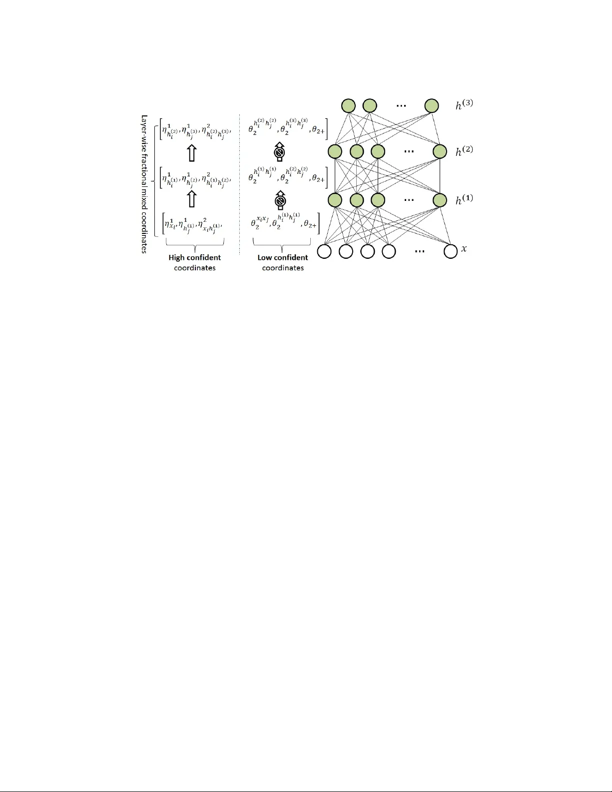
Understanding Boltzmann Mac hine and Deep Learning via A Conﬁden t Information First Principle Xiaozhao Zhao 0.25eye@gmail.com Scho ol of Computer Scienc e and T e chnolo gy, Tianjin University Tianjin, 300072, China Y uexian Hou krete1941@gmail.com Scho ol of Computer Scienc e and T e chnolo gy, Tianjin University Tianjin, 300072, China Qian Y u yqcloud@gmail.com Scho ol of Computer Softwar e, Tianjin University Tianjin, 300072, China Da w ei Song da wei.song2010@gmail.com Scho ol of Computer Scienc e and T e chnolo gy, Tianjin University Tianjin, 300072, China and Dep artment of Computing, The Op en University Milton Keynes, MK7 6AA, UK W enjie Li cswjli@comp.pol yu.edu.hk Dep artment of Computing, The Hong Kong Polyte chnic University Hung Hom, Kow lo on, Hong Kong, China Editor: Abstract T ypical dimensionalit y reduction methods fo cus on directly reducing the n umber of ran- dom v ariables while retaining maximal v ariations in the data. In this pap er, we consider the dimensionalit y reduction in parameter spaces of binary m ultiv ariate distributions. W e prop ose a general Conﬁden t-Information-First (CIF) principle to maximally preserve pa- rameters with conﬁdent estimates and rule out unreliable or noisy parameters. F ormally , the conﬁdence of a parameter can b e assessed by its Fisher information, which establishes a connection with the inv erse v ariance of any unbiased estimate for the parameter via the Cram ´ er-Rao b ound. W e then revisit Boltzmann machines (BM) and theoretically show that both single-lay er BM without hidden units (SBM) and restricted BM (RBM) can b e solidly derived using the CIF principle. This can not only help us uncov er and formalize the essen tial parts of the target density that SBM and RBM capture, but also suggest that the deep neural net work consisting of several la yers of RBM can b e seen as the lay er- wise application of CIF. Guided by the theoretical analysis, we develop a sample-sp eciﬁc CIF-based contrastiv e div ergence (CD-CIF) algorithm for SBM and a CIF-based iterative pro jection pro cedure (IP) for RBM. Both CD-CIF and IP are studied in a series of densit y estimation exp eriments. Keyw ords: Boltzmann Machine, Deep Learning, Information Geometry , Fisher Informa- tion, Parametric Reduction 1 1. In tro duction Recen tly , deep learning mo dels (e.g., Deep Belief Net works (DBN)(Hin ton and Salakhut- dino v, 2006), Stac ked Denoising Auto-enco der (Ranzato et al., 2006), Deep Boltzmann Mac hine (DBM) (Salakhutdino v and Hinton, 2012) and etc.) hav e drawn increasing atten- tion due to their impressive results in v arious application areas, such as computer vision (Bengio et al., 2006; Ranzato et al., 2006; Osindero and Hin ton, 2007), natural language pro- cessing (Collob ert and W eston, 2008) and information retriev al (Salakh utdinov and Hin ton, 2007a,b). Despite of these practical successes, there hav e be en debates on the fundamental principle of the design and training of those deep architectures. One imp ortant problem is the unsup ervise d pr e-tr aining , whic h w ould ﬁt the parameters to b etter capture the structure in the input distribution (Erhan et al., 2010). F rom the probabilistic mo deling p ersp ective, this pro cess can b e interpreted as an attempt to reco ver a set of mo del parameters for a generativ e neural net work that w ould well describ e the distribution underlying the observ ed high-dimensional data. In general, to suﬃcien tly depict the original high-dimensional data requires a high-dimensional parameter space. How ev er, ov erﬁtting usually o ccur when the mo del is excessively complex. On the other hand, Dauphin and Bengio (2013) empirically sho ws the failure of some big neural netw orks in lev eraging the added capacity to reduce underﬁtting. Hence it is imp ortant to uncov er and understand what the ﬁrst principle would b e on r e ducing the dimensionality of the p ar ameter sp ac e c onc erning the sample size . This ques- tion is also recognized b y Erhan et al. (2010). They empirically show that the unsup ervised pre-training acts as a regularization on parameters in a w ay that the parameters are set in a region, from whic h better basins of attraction can b e reac hed. The regularization on param- eters could b e seen as a kind of dimensionality reduction pro cedure on parameter spaces b y restricting those parameters in a desired region. Ho wev er, the in trinsic mechanisms b ehind the regularization process are still unclear. Th us, further theoretical justiﬁcations are needed in order to formally analyze what the essential parts of the target density that the neural net works can capture. An indepth in vestigation into this question will lead to t wo signiﬁcan t results: 1) a formal explanation on what exactly the neural net works w ould p erform in the pre-training pro cess; 2) some theoretical insigh ts on how to do it b etter. Duin and Pe¸ ek alsk a (2006) empirically sho w that the sampling densit y of a giv en dataset and the resulting complexit y of a learning problem are closely interrelated. If the initial sampling density is insuﬃcien t, this may result in a preferred mo del of a low er complexit y , so that w e hav e a satisfactory sampling to estimate mo del parameters. On the other hand, if the n umber of samples is originally abundan t, the preferred mo del ma y b ecome more complex so that we could hav e represented the dataset in more details. Moreo ver, this connection b ecomes more complicated if the observed samples contain noises. No w the obstacle is ho w to incorporate this relationship b et w een the dataset and the preferred model in to the learning pro cess. In this paper, we mainly fo cus on analyzing the Boltzmann mac hines, the main building blo cks of many neural net works, from a nov el information geometry (IG)(Amari and Nagaok a, 1993) p erspective. Assuming there exists an ideal parametric mo del S that is general enough to represen t all system phenomena, our goal of the parametric reduction is to derive a lo wer-dimensional sub-mo del M for a giv en dataset (usually insuﬃcient or p erturb ed b y noises) b y reducing 2 the num b er of free parameters in S . In this pap er, w e prop ose a Conﬁdent-Information- First (CIF) principle to maximally preserve the parameters with highly conﬁdent estimates and rule out the unreliable or noisy parameters with resp ect to the density estimation of binary m ultiv ariate distributions. F rom the IG p oint of view, the c onﬁdenc e 1 of a parameter can b e assessed by its Fisher information (Amari and Nagaok a, 1993), which establishes a connection with the inv erse v ariance of an y un biased estimate for the considered parameter via the Cram ´ er-Rao b ound (see Rao, 1945). It is worth emphasizing that the prop osed CIF as a principle of parametric reduction is fundamen tally diﬀeren t from the traditional feature reduction (or feature extraction) metho ds (F o dor, 2002; Lee and V erleysen, 2007). The latter fo cus on directly reducing the dimensionality on feature space by retaining maximal v ariations in the data, e.g., Principle Comp onents Analysis (PCA) (Jolliﬀe, 2002), while CIF oﬀers a principled metho d to deal with high-dimensional data in the parameter spaces by a strategy that is universally deriv ed from the ﬁrst principle, indep enden t of the geometric metric in the feature spaces. The CIF tak es an information-orien ted viewp oin t of statistical mac hine learning. The information 2 is ro oted on the v ariations (or ﬂuctuations) in the imp erfe ct observ ations (due to insuﬃcien t sampling, noise and intrinsic limitations of the “observ er”) and trans- mits throughout the whole learning pro cess. This idea is also well recognized in mo dern ph ysics, as stated in Wheeler (1994): “All things ph ysical are information-theoretic in ori- gin and this is a participatory universe...Observ er participancy gives rise to information; and information gives rise to physics.”. F ollowing this viewp oint, F rieden (2004) uniﬁes the deriv ation of ph ysical laws in ma jor ﬁelds of ph ysics, from the Dirac equation to the Maxw ell-Boltzmann v elo city disp ersion law, using the extreme physical information princi- ple (EPI). The information used in this uniﬁcation is exactly the Fisher information (Rao, 1945), which measures the quality of any measuremen t(s). In terms of statistical machine learning, the aim of this pap er is of tw o folds: a) to incorp orate the Fisher information in to the mo delling of the in trinsic v ariations in the data that give rise to the desired mo del, by using the IG framework (Amari and Nagaok a, 1993); b) to sho w b y examples that some existing probabilistic mo dels, e.g., SBM and RBM, comply with the CIF principle and can b e deriv ed from it. The main contributions are: 1. W e prop ose a gener al CIF principle for parameter reduction to maximally preserve the parameters of high conﬁdence and eliminate the unreliable parameters of binary m ultiv ariate distributions in the framework of IG. W e also give a geometric in terpre- tation of CIF by showing that it can maximally preserv e the exp ected information distance. 2. The implemen tation of CIF, that is, the deriv ation of probabilistic mo dels, is illus- trated b y revisiting tw o widely used Boltzmann machines, i.e., Single la yer BM with- out hidden units (SBM) and restricted BM (RBM). And the deep neural netw ork consisting of several la yers of RBM can b e seen as the lay er-by-la y er application of CIF. 1. Note that, in this pap er, the meaning of conﬁdenc e is diﬀerent from the common concept de gr e e of c onﬁdence in statistics. 2. There are many kinds of “information” deﬁned for a probability distribution p ( x ), e.g., entrop y , Fisher information. The en tropy is a global measure of smo othness in p ( x ). Fisher information is a local measure that is sensitive to local rearrangemen t of p oints ( x, p ( x )). 3 3. Based on the ab ov e theoretical analysis, a CIF-based iterativ e pro jection pro cedure (IP) inherent in the learning of RBM is unco vered. And traditional gradient-based metho ds, e.g., maximum-lik eliho o d (ML) and contrastiv e div ergence (CD) (Carreira- P erpinan and Hinton, 2005), can b e seen as appro ximations of IP . Exp erimental results indicate that IP is more robust against sampling biases, due to its separation of the p ositiv e sampling pro cess and the gradien t estimation. 4. Beyond the general CIF, we prop ose a sample-sp e ciﬁc CIF and in tegrate it in to the CD algorithm for SBM to conﬁne the parameter space to a conﬁdent parameter region indicated b y samples. It leads to a signiﬁcant improv ement in a series of density estimation exp eriments, when the sampling is insuﬃcien t. The rest of the paper is organized as follows: Section 2 introduces some preliminaries of IG. Then the general CIF principle is prop osed in Section 3. In Section 4, we analyze tw o implemen tations of CIF using the BM with and without hidden units, i.e., SBM and RBM. After that, a sample-speciﬁc CIF-based CD learning method (CD-CIF) for SBM and a CIF- based iterative pro jection procedure for RBM are prop osed and exp erimentally studied in Section 5. Finally , we draw conclusions and highlight some future research directions in Section 6. 2. Theoretical F oundations of Information Geometry In this section, w e in tro duce and dev elop the theoretical foundations of Information Geome- try (IG) (Amari and Nagaok a, 1993) for the manifold S of binary multiv ariate distributions with a giv en n umber of v ariables n , i.e., the op en simplex of all probability distributions o ver binary vector x ∈ { 0 , 1 } n . This will lay the foundation for our theoretical deviation of the gener al CIF . 2.1 Notations for Manifold S In IG, a family of probabilit y distributions is considered as a diﬀerentiable manifold with certain parametric co ordinate systems. In the case of binary multiv ariate distributions, four basic co ordinate systems are often used: p -co ordinates, η -co ordinates, θ -co ordinates and mixed-co ordinates (Amari and Nagaok a, 1993; Hou et al., 2013). Mixed-co ordinates is of vital imp ortance for our analysis. F or the p -co ordinates [ p ] with n binary v ariables, the probabilit y distribution ov er 2 n states of x can b e completely sp eciﬁed by any 2 n − 1 p ositive num b ers indicating the probabilit y of the corresp onding exclusive states on n binary v ariables. F or example, the p -co ordinates of n = 2 v ariables could b e [ p ] = ( p 01 , p 10 , p 11 ). Note that IG requires all probabilit y terms to b e p ositive. F or simplicity , we use the capital letters I , J, . . . to index the co ordinate parameters of probabilistic distribution. An index I can b e regarded as a subset of { 1 , 2 , . . . , n } . And p I stands for the probabilit y that all v ariables indicated by I equal to one and the complemented v ariables are zero. F or example, if I = { 1 , 2 , 4 } and n = 4, then p I = p 1101 = P rob ( x 1 = 1 , x 2 = 1 , x 3 = 0 , x 4 = 1). Note that the null set can also b e a legal index of the p -co ordinates, whic h indicates the probabilit y that all v ariables are zero, denoted as p 0 ... 0 . 4 Another co ordinate system often used in IG is η -co ordinates, whic h is deﬁned b y: η I = E [ X I ] = P rob { Y i ∈ I x i = 1 } (1) where the v alue of X I is giv en by Q i ∈ I x i and the exp ectation is taken with resp ect to the probabilit y distribution ov er x . Grouping the co ordinates by their orders, η -co ordinate system is denoted as [ η ] = ( η 1 i , η 2 ij , . . . , η n 1 , 2 ...n ), where the sup erscript indicates the order n umber of the corresp onding parameter. F or example, η 2 ij denotes the set of all η parameters with the order num b er 2. The θ -co ordinates (natural co ordinates) is deﬁned by: log p ( x ) = X I ⊆{ 1 , 2 ,...,n } ,I 6 = N ul lS et θ I X I − ψ (2) where ψ = − log P r ob { x i = 0 , ∀ i ∈ { 1 , 2 , ..., n }} . The θ -co ordinate is denoted as [ θ ] = ( θ i 1 , θ ij 2 , . . . , θ 1 ,...,n n ), where the subscript indicates the order n umber of the corresp onding parameter. Note that the order indices lo cate at diﬀerent p ositions in [ η ] and [ θ ] following the conv ention in Amari et al. (1992). The relation b et w een co ordinate systems [ η ] and [ θ ] is bijectiv e (Amari et al., 1992). More formally , they are connected by the Legendre transformation: θ I = ∂ φ ( η ) ∂ η I , η I = ∂ ψ ( θ ) ∂ θ I (3) where ψ ( θ ) and φ ( η ) meet the following iden tit y ψ ( θ ) + φ ( η ) − X θ I η I = 0 (4) The function ψ ( θ ) is introduced in Eq. (2): ψ ( θ ) = log ( X x exp { X I θ I X I ( x ) } ) (5) and hence φ ( η ) is the negative of entrop y: φ ( η ) = X x p ( x ; θ ( η )) log p ( x ; θ ( η )) (6) Next we introduce mixed-co ordinates, which is imp ortant for our deriv ation of CIF. In general, the manifold S of probability distributions could b e represen ted by the l -mixed- co ordinates (Amari et al., 1992): [ ζ ] l = ( η 1 i , η 2 ij , . . . , η l i,j,...,k , θ i,j,...,k l +1 , . . . , θ 1 ,...,n n ) (7) where the ﬁrst part consists of η -co ordinates with order less or equal to l (denoted by [ η l − ]) and the second part consists of θ -co ordinates with order greater than l (denoted by [ θ l + ]), l ∈ { 1 , ..., n } . 5 2.2 Fisher Information Matrix for Parametric Co ordinates F or a general co ordinate system [ ξ ], the i th-ro w and j th-col element of the Fisher informa- tion matrix for [ ξ ] (denoted b y G ξ ) is deﬁned as the co v ariance of the scores of [ ξ i ] and [ ξ j ] (Rao, 1945), i.e., g ij = E [ ∂ log p ( x ; ξ ) ∂ ξ i · ∂ log p ( x ; ξ ) ∂ ξ j ] The Fisher information measures the amount of information in the data that a statistic carries ab out the unknown parameter (Kass, 1989). The Fisher information matrix is of vital imp ortance to our analysis b ecause the inv erse of Fisher information matrix gives an asymptotically tight low er bound of the co v ariance matrix of any unbiased estimate for the considered parameters (Rao, 1945). Moreov er, the Fisher information matrix, as a distance metric, is in v ariant to re-paramete rization (Rao, 1945), and can b e pro ved to b e the unique metric that is inv ariant to the map of random v ariables corresponding to a suﬃcien t statistic (Amari et al., 1992; Chen tsov, 1982). Another imp ortan t concept related to our analysis is the ortho gonality deﬁned b y Fisher information. Tw o co ordinate parameters ξ i and ξ j are called ortho gonal if and only if their Fisher information v anishes, i.e., g ij = 0, meaning that their inﬂuences to the log likelihoo d function are uncorrelated. A more technical meaning of orthogonalit y is that the maximum likeliho o d estimates (MLE) of orthogonal parameters can b e indep enden tly p erformed. The Fisher information for [ θ ] can be rewritten as g I J = ∂ 2 ψ ( θ ) ∂ θ I ∂ θ J , and for [ η ] it is g I J = ∂ 2 φ ( η ) ∂ η I ∂ η J (Amari and Nagaok a, 1993). Let G θ = ( g I J ) and G η = ( g I J ) b e the Fisher information matrices for [ θ ] and [ η ] resp ectively . It can b e shown that G θ and G η are mutu- ally inv erse matrices, i.e., P J g I J g J K = δ I K , where δ I K = 1 if I = K and 0 otherwise (Amari and Nagaok a, 1993). In order to generally compute G θ and G η , w e develop the follo wing Proposition 1 and 2. Note that Prop osition 1 is a generalization of Theorem 2 in Amari et al. (1992). Prop osition 1 The Fisher information b etwe en two p ar ameters θ I and θ J in [ θ ] , is given by g I J ( θ ) = η I S J − η I η J (8) Pro of in App endix A.1 Prop osition 2 The Fisher information b etwe en two p ar ameters η I and η J in [ η ] , is given by g I J ( η ) = X K ⊆ I ∩ J ( − 1) | I − K | + | J − K | · 1 p K (9) wher e | · | denotes the c ar dinality op er ator. Pro of in App endix A.2 F or example, let [ p ] = ( p 001 , p 010 , p 011 , p 100 , p 101 , p 110 , p 111 ) b e the p -co ordinates of a proba- bilit y distribution with three v ariables. Then, the Fisher information of η I and η J can b e calculated based on Equation (9): if I = { 1 , 2 } and J = { 2 , 3 } , g I J = 1 p 000 + 1 p 010 , and if I = { 1 , 2 } and J = { 1 , 2 , 3 } , g I J = − ( 1 p 000 + 1 p 010 + 1 p 100 + 1 p 110 ), etc. 6 3. The General CIF Principle F or P arametric Reduction As describ ed in Section 2.1, the general manifold S of all probabilit y distributions ov er binary vector x ∈ { 0 , 1 } n , could b e exactly represen ted using the parametric co ordinate systems of dimensionalit y 2 n − 1. Ho wev er, giv en the limited samples generated from a tar- get distribution, it is almost infeasible to determine its co ordinates in suc h high-dimensional parameter space with acceptable accuracy and in reasonable time. Giv en a target distri- bution q ( x ) on the general manifold S , we consider the problem of realizing it by a low er- dimensionalit y submanifold. This is deﬁned as the problem of parametric reduction for m ultiv ariate binary distributions. 3.1 The General CIF Principle In this section, we will formally illuminate the general CIF for parametric reduction. Intu- itiv ely , if we can construct a co ordinate system so that the conﬁdences (measured by Fisher information) of its parameters entail a natural hierarc hy , in whic h high conﬁden t parame- ters can b e signiﬁcantly distinguished from low conﬁdent ones, then the general CIF can be con venien tly implemen ted by keeping the high conﬁden t parameters unc hanging and setting the lowly conﬁdent parameters to neutral v alues. How ever, the c hoice of co ordinates (or equiv alently , parameters) in CIF is crucial to its usage. This strategy is infeasible in terms of p -co ordinates, η -co ordinates or θ -coordinates, since it is easy to see that the hierarchies of conﬁdences in these co ordinate systems are far from signiﬁcant, as sho wn b y an example later in this section. The following prop ositions show that mixed-co ordinates meet the requiremen t realizing the general CIF. Let [ ζ ] l b e the mixed-co ordinates deﬁned in Section 2.1. Proposition 3 giv es a closed form for calculating the Fisher information matrix G ζ . Prop osition 3 The Fisher information matrix of the l -mixe d-c o or dinates [ ζ ] l is given by: G ζ =  A 0 0 B  (10) wher e A = (( G − 1 η ) I η ) − 1 , B = (( G − 1 θ ) J θ ) − 1 , G η and G θ ar e the Fisher information matric es of [ θ ] and [ ζ ] l , r esp e ctively, and I η is the index of the p ar ameters shar e d by [ η ] and [ ζ ] l , i.e., { η 1 i , ..., η l ij } , and J θ is the index set of the p ar ameters shar e d by [ θ ] and [ ζ ] l , i.e., { θ i,j,...,k l +1 , . . . , θ 1 ,...,n n } . Pro of in App endix A.3. Prop osition 4 The diagonal of A ar e lower b ounde d by 1 , and that of B ar e upp er b ounde d by 1 . Pro of in App endix A.4. According to Prop osition 3 and Prop osition 4, the conﬁdences of coordinate parameters in [ ζ ] l en tail a natural hierarch y: the ﬁrst part of high conﬁdent parameters [ η l − ] are sep- arated from the second part of low conﬁden t parameters [ θ l + ], whic h has a neutral v alue (zero). Moreo ver, the parameters in [ η l − ] is orthogonal to the ones in [ θ l + ], indicating that 7 Figure 1: By pro jecting a p oin t q ( x ) on S to a submanifold M , the l -tailored-mixed- co ordinates [ ζ ] l t giv es a desirable M that maximally preserve the expected Fisher information distance when pro jecting a ε -neighborho o d cen tered at q ( x ) onto M . w e could estimate these tw o parts indep enden tly (Hou et al., 2013). Hence we can imple- men t the general CIF principle for parametric reduction in [ ζ ] l b y replacing low conﬁdent parameters with neutral v alue zeros and reconstructing the resulting distribution. It turns out that the submanifold tailored b y CIF b ecomes [ ζ ] l t = ( η 1 i , ..., η l ij...k , 0 , . . . , 0). W e call [ ζ ] l t the l -tailored-mixed-co ordinates. T o grasp an intuitiv e picture for the general CIF strategy and its signiﬁcance w.r.t mixed-co ordinates, let us consider an example with [ p ] = ( p 001 = 0 . 15 , p 010 = 0 . 1 , p 011 = 0 . 05 , p 100 = 0 . 2 , p 101 = 0 . 1 , p 110 = 0 . 05 , p 111 = 0 . 3). Then the conﬁdences for co ordinates in [ η ], [ θ ] and [ ζ ] 2 are given b y the diagonal elements of the corresp onding Fisher informa- tion matrices. Applying the 2-tailored CIF in mixed-coordinates, the loss ratios of Fisher information is 0 . 001%, and the ratio of the Fisher information of the tailored parameter ( θ 123 3 ) to the remaining η parameter with the smallest Fisher information is 0 . 06%. On the other hand, the ab o ve tw o ratios b ecome 7 . 58% and 94 . 45% (in η -coordinates) or 12 . 94% and 92 . 31% (in θ -co ordinates), resp ectively . Next, w e will restate the CIF principle in terms of the geometric p ersp ective of sub- manifold pro jection. Let M b e a smo oth submanifold in S . Giv en a p oint q ( x ) ∈ S , the pro jection of q ( x ) to M is the p oin t p ( x ) that b elongs to M and is closest to q ( x ) in the sense of the Kullbac k-Leibler div ergence (K-L div ergence) from the distribution q ( x ) to p ( x ) (Amari et al., 1992): D ( q ( x ) , p ( x )) = X x q ( x ) log q ( x ) p ( x ) (11) Alternativ ely , since K-L div ergence is not symmetric, the pro jection of q ( x ) to M can also b e deﬁned as the point p ( x ) ∈ M that minimizes the K-L divergence from M to q ( x ). In the rest of this pap er, the direction of the K-L divergence used in a particular pro jection is explicitly sp eciﬁed when there is an am biguity . 8 The CIF en tails a submanifold of S via the l -tailored-mixed-co ordinates [ ζ ] l t . Ho wev er, there exist many diﬀerent submanifolds of S . Now our question is: do es ther e exist a gener al criterion to distinguish which pr oje ction is b est? If such principle do es exist, is CIF the right one? The follo wing prop osition shows that the general CIF entails a geometric in terpretation illuminated in Figure 1, whic h w ould lead to an optimal submanifold M . 3 Prop osition 5 Given a statistic al manifold S in l -mixe d-c o or dinates [ ζ ] l , let the c orr e- sp onding l -tailor e d-mixe d-c o or dinates [ ζ ] l t has k fr e e p ar ameters. Then, among al l k -dimensional submanifolds of S , the submanifold determine d by [ ζ ] l t c an maximal ly pr eserve the exp e cte d information distanc e induc e d by Fisher-R ao metric. Pro of in App endix A.5. 4. Tw o Implementations of CIF using Boltzmann Machine In previous section, a general CIF is unco vered in the [ ζ ] l co ordinates for m ultiv ariate binary distributions. Now w e consider the implemen tations of CIF when l equals to 2 using the Boltzmann machines (BM). More sp eciﬁcally , we sho w that tw o kinds of BMs, i.e., the single la yer BM without hidden units (SBM) and the restricted BM (RBM), are indeed instances following the general CIF principle. F or eac h case, the application of CIF can b e in terpreted in tw o p ersp ectives: an algebraic and geometric interpretation. 4.1 Neural Netw orks as Parametric Reduction Model Man y neural netw orks with ﬁxed arc hitecture, suc h as SBM, RBM, high-order BM (Albizuri et al., 1995), deep b elief net works (Hinton and Salakh utdinov, 2006), ha v e b een prop osed to appro ximately realize the underlying distributions in diﬀeren t application scenarios. Those neural netw orks are designed to fulﬁll the parametric reduction for certain tasks by specify- ing the n umber of adjustable parameters, namely the num b er of connection weigh ts and the n umber of biases. W e b elieve that there exists a general criterion to design the structure of neural submanifolds for the particular application in hand, and the problem of parametric reduction is equiv alen t to the choice of submanifolds. Next, we will brieﬂy introduce the general BM and the gradien t-based learning algorithm. 4.1.1 Intr oduction To The Bol tzmann Ma chines In general, a BM (Ackley et al., 1985) is deﬁned as a sto chastic neural net work consisting of visible units x ∈ { 0 , 1 } n x and hidden units h ∈ { 0 , 1 } n h , where each unit ﬁres sto c hastically dep ending on the weigh ted sum of its inputs. The energy function is deﬁned as follows: E B M ( x, h ; ξ ) = − 1 2 x T U x − 1 2 h T V h − x T W h − b T x − d T h (12) 3. Note that the CIF is related to but fundamen tally diﬀeren t from the m -pro jection in Amari et al. (1992). Amari et al. (1992) fo cuses on the problem of pro jecting a p oint Q on S to the submanifold of BM and sho ws that m -pro jection is the p oint on BM that is closest to Q . Actually , the m -pro jection is a special case of our [ ζ ] l t -pro jection when l is 2. In the present pap er, we fo cus on the problem of developing a general criterion that could help us ﬁnd the optimal submanifold to pro ject on. 9 where ξ = { U, V , W , b, d } are the parameters: visible-visible interactions ( U ), hidden-hidden in teractions ( V ), visible-hidden interactions ( W ), visible self-connections ( b ) and hidden self- connections ( d ). The diagonals of U and V are set to zero. W e can express the Boltzmann distribution ov er the joint space of x and h as b elow: p ( x, h ; ξ ) = 1 Z exp {− E B M ( x, h ; ξ ) } (13) where Z is a normalization factor. Let B b e the set of Boltzmann distributions realized b y BM. Actually , B is a submanifold of the general manifold S xh o ver { x, h } . F rom Equation (13) and (12), we can see that ξ = { U, V , W , b, d } pla ys the role of B ’s co ordinates in θ -co ordinates (Equation 2) as follo ws: θ 1 : θ x i 1 = b x i , θ h j 1 = d h j ( ∀ x i ∈ x, h j ∈ h ) θ 2 : θ x i x j 2 = U x i ,x j , θ x i h j 2 = W x i ,h j , θ h i h j 2 = V h i ,h j ( ∀ x i , x j ∈ x ; h i , h j ∈ h ) θ 2+ : θ x i ...x j h u ...h v m = 0 , m > 2 , ( ∀ x i , . . . , x j ∈ x ; h u , . . . , h v ∈ h ) (14) So the θ -co ordinates for BM is giv en by: [ θ ] B M = ( θ x i 1 , θ h j 1 | {z } 1 − order , θ x i x j 2 , θ x i h j 2 , θ h i h j 2 | {z } 2 − order , 0 , . . . , 0 | {z } order s> 2 ) . (15) The SBM and RBM are sp ecial cases of the general BM. Since SBM has n h = 0 and all the visible units are connected to eac h other, the parameters of SBM are ξ sbm = { U, b } and { V , W, d } are all set to zero. F or RBM, it has connections only b etw een hidden and visible units. Thus, the parameters of RBM are ξ rbm = { W , b, d } and { U, V } are set to zero. 4.1.2 F ormula tion on the Gradient-based Learning of BM Giv en the sample x that generated from the underlying distribution, the maximum-likeliho o d (ML) is commonly used gradient ascen t metho d for training BM in order to maximize the log-lik eliho o d log p ( x ; ξ ) of the parameters ξ (Carreira-Perpinan and Hinton, 2005). Based on Equation (13), the log-lik eliho o d is given as follows: log p ( x ; ξ ) = log X h e − E ( x,h ; ξ ) − log X x 0 ,h 0 e − E ( x 0 ,h 0 ; ξ ) Diﬀeren tiating the log-likelihoo d, the gradient v ector with resp ect to ξ is as follows: ∂ log p ( x ; ξ ) ∂ ξ = X h p ( h | x ; ξ ) ∂ [ − E ( x, h ; ξ )] ∂ ξ − X x 0 ,h 0 p ( h 0 | x 0 ; ξ ) ∂ [ − E ( x 0 , h 0 ; ξ )] ∂ ξ (16) The ∂ E ( x,h ; ξ ) ∂ ξ can b e easily calculated from Equation (12). Then we can obtain the sto c hastic gradien t using Gibbs sampling (Gilks et al., 1996) in tw o phases: sample h giv en x for the ﬁrst term, called the p ositive phase, and sample ( x 0 , h 0 ) from the stationary distribution p ( x 0 , h 0 ; ξ ) for the second term, called the negative phase. Now with the resulting sto chastic gradien t estimation, the learning rule is to adjust ξ by: ∆ ξ = ε · ∂ log p ( x ; ξ ) ∂ ξ = ε · ( −h ∂ E ( x, h ; ξ ) ∂ ξ i 0 + h ∂ E ( x 0 , h 0 ; ξ ) ∂ ξ i ∞ ) (17) 10 where ε is the learning rate, h·i 0 denotes the av erage using the sample data and h·i ∞ denotes the a verage with resp ect to the stationary distribution p ( x, h ; ξ ) after the corresp onding Gibbs sampling phases. 4 In follo wing sections, w e will revisit tw o special BM, namely SBM and RBM, and theo- retically show that b oth SBM and RBM can b e derived using the CIF principle. This helps us formalize what essential parts of the target density the SBM and RBM capture. 4.2 The CIF-based Deriv ation of Boltzmann Machine without Hidden Units Giv en an y underlying probabilit y distribution q ( x ) on the general manifold S o v er { x } , the logarithm of q ( x ) can b e represen ted b y a linear decomp osition of θ -co ordinates as shown in Equation (2). Since it is impractical to recognize all co ordinates for the target distri- bution, we would like to only appro ximate part of them and end up with a k -dimensional submanifold M of S , where k (  2 n x − 1) is the nu mber of free parameters. Here, we set k to b e the same dimensionalit y as SBM, i.e., k = n x ( n x +1) 2 , so that all candidate subman- ifolds are comparable to the submanifold endo wed b y SBM (denoted as M sbm ). Next, the rationale underlying the design of M sbm can b e illuminated using the general CIF from t wo p ersp ectives, algebraically and geometrically . 4.2.1 SBM as 2-t ailored-mixed-coordina tes Let the 2-mixed-co ordinates of q ( x ) on S b e [ ζ ] 2 = ( η 1 i , η 2 ij , θ i,j,k 3 , . . . , θ 1 ,...,n x n x ). Applying the general CIF on [ ζ ] 2 , our parametric reduction rule is to preserv e the high conﬁdent part parameters [ η 2 − ] and replace low conﬁdent parameters [ θ 2+ ] with a ﬁxed neutral v alue zero. Thus we deriv e the 2-tailored-mixed-co ordinates: [ ζ ] 2 t = ( η 1 i , η 2 ij , 0 , . . . , 0), as the optimal approximation of q ( x ) b y the k -dimensional submanifolds. On the other hand, giv en the 2-mixed-co ordinates of q ( x ), the pro jection p ( x ) ∈ M sbm of q ( x ) is pro v ed to b e [ ζ ] p = ( η 1 i , η 2 ij , 0 , . . . , 0) (Amari et al., 1992). Thus, SBM deﬁnes a probabilistic parameter space that is exactly deriv ed from CIF. 4.2.2 SBM as Maximal Informa tion Dist ance Projection Next corollary , following Prop osition 5, sho ws a geometric deriv ation of SBM. W e mak e it explicit that the pro jection on M sbm could maximally preserve the exp ected information distance comparing to other tailored submanifolds of S with the same dimensionality k . Corollary 6 Given the gener al manifold S in 2 -mixe d-c o or dinates [ ζ ] 2 , SBM deﬁnes an k - dimensional submanifold of S that c an maximal ly pr eserve the exp e cte d information distanc e induc e d by Fisher-R ao metric. Pro of in App endix A.6. F rom the CIF-based deriv ation, we can see that SBM conﬁnes the statistical manifold in the parameter subspace spanned b y those directions with high conﬁdences, whic h is prov ed to maximally preserv e the exp ected information distance. 4. Both the tw o special BMs, i.e., SBM and RBM, can b e trained using the ML method. Note that SBM has no hidden units and hence no positive sampling is needed in training SBM. 11 4.2.3 The Rela tion Between [ ζ ] 2 t and the ML Learning of SBM T o learn suc h [ ζ ] 2 t , we need to learn the parameters ξ of SBM such that its stationary distribution preserv es the same co ordinates [ η 2 − ] as target distribution q ( x ). Actually , this is exactly what traditional gradient-based learning algorithms in tend to do to train SBM. Next prop osition shows that the ML metho d for training SBM is equiv alent to learn the tailored 2-mixed co ordinates [ ζ ] 2 t . Prop osition 7 Given the tar get distribution q ( x ) with 2-mixe d c o or dinates: [ ζ ] 2 = ( η 1 i , η 2 ij , θ 2+ ) , the c o or dinates of the SBM with stationary distribution q ( x ; ξ ) , le arnt by ML, ar e uniquely given by [ ζ ] 2 t = ( η 1 i , η 2 ij , θ 2+ = 0) Pro of in App endix A.7. 4.3 The CIF-based Deriv ation of Restricted Boltzmann Machine In previous section, the general CIF unco vers why SBM uses the co ordinates up to 2 nd - order, i.e., preserv es the η -coordinates of the 1 st -order and 2 nd -order. In this section, we will in v estigate the cases where hidden units are introduced. P articularly , one of the fun- damen tal problem in neural net work researc h is the unsup ervised represen tation learning (Bengio et al., 2013), which attempts to c haracterize the underlying distribution through the discov ery of a set of latent v ariables (or features). Man y algorithmic mo dels hav e b een prop osed, suc h as restricted Boltzmann machine (RBM) (Hinton and Salakh utdinov, 2006) and auto-enco ders (Rifai et al., 2011; Vincen t et al., 2010), for learning one level of feature extraction. Then, in deep learning mo dels, the representation learnt at one level is used as input for learning the next lev el, etc. Ho wev er, some imp ortant questions remain to be clar- iﬁed: Do these algorithms implicitly learn ab out the whole densit y or only some aspects? If they c aptur e the essenc e of the tar get density, then c an we formalize the link b etwe en the essential p art and omitte d p art? This section will try to answer these questions using CIF. 4.3.1 Tw o Necessar y Conditions f or Represent a tion Learning In terms of one level feature extraction, there are tw o main principles that guide a go o d represen tation learning: • Comp actness of represen tation: minimize the redundancy b etw een hidden v ariables in the represen tation 5 . • Completeness of reconstruction: the learnt represen tation captures suﬃcient informa- tion in the input, and could completely reconstruct input distribution, in a statistical sense. 5. The concept of compactness in the neural netw ork is of tw o-folds. 1) mo del-scale compactness: a restriction on the num b er of hidden units in order to give a parsimonious representation w.r.t underlying distribution; 2) structural compactness: a restriction on how hidden units are connected suc h that the redundancy in the hidden representation is minimized. In this pap er, w e mainly fo cus on the latter case. 12 Let S xh b e the general manifold of probability distributions ov er the joint space of visible units x and hidden units h , and S x b e the general manifold o ver visible units x . Giv en an y observ ation distribution q ( x ) ∈ S x , our problem is to ﬁnd the p ( x, h ) ∈ S xh with the mar ginal distribution p ( x ) that b est appr oximates q ( x ) , while p ( x, h ) is c onsistent with the c omp actness and c ompleteness c onditions . Here, the K-L divergence, deﬁned in Equation (11), is used as the criterion of appro ximation. First, we will inv estigate the submanifold of join t distributions p ( x, h ) ∈ S xh that fulﬁll the ab ov e tw o conditions. Let us denote this submanifold as M cc . Extending Equation (2) to manifold S xh , p ( x, h ) has the θ -co ordinates deﬁned by: log p ( x, h ) = X I ⊆{ x,h } & I 6 = N ul lS et θ I X I − ψ (18) F or the c ompleteness requiremen t, it is easy to prov e that the probability of any input v ariable x i can b e fully determined only by the giv en hidden representation and independent with remainng input v ariables x j ( j 6 = i ), if and only if θ I = 0 for an y I that con tains t w o or more input v ariables in Equation (18). Similarly , the c omp actness corresp onds to the extraction of statistically indep endent hidden v ariables given the input, i.e., θ I = 0 for an y I that con tains t w o or more hidden v ariables in Equation (18). Then M cc is given by the follo wing co ordinate system: [ θ ] cc = ( θ x i 1 , θ h j 1 | {z } 1 − order , θ x i x j 2 = 0 , θ x i h j 2 , θ h i h j 2 = 0 | {z } 2 − order , 0 , . . . , 0 | {z } order s> 2 ) . (19) Then our problem is restated as to ﬁnd the p ( x, h ) ∈ M cc with the mar ginal distribution p ( x ) that b est appr oximates q ( x ). 4.3.2 The Equiv alence between RBM and M cc RBM is a sp ecial kind of BM that restricts the in teractions in Equation (12) only to those b et ween hidden and visible units, i.e., U x i ,x j = 0 , V h i ,h j = 0 ∀ x i , x j ∈ x ; h i , h j ∈ h . Let ξ rbm = { W , b, d } denotes the set of parameters in RBM. Th us, the θ -co ordinates for RBM can b e deriv ed directly from Equation (15): [ θ ] RB M = ( θ x i 1 , θ h j 1 | {z } 1 − order , θ x i x j 2 = 0 , θ x i h j 2 , θ h i h j 2 = 0 | {z } 2 − order , 0 , . . . , 0 | {z } order s> 2 ) (20) Comparing Equation (19) to (20), the submanifold M rbm deﬁned b y RBM is equiv alent with M cc since they share exactly the same co ordinate system. This indicates that the c omp actness and c ompleteness conditions is indeed realized by RBM. W e use a simpler notation B to denote M rbm . Next, w e will show how to use CIF to in terpret the training pro cess of RBM. 4.3.3 The CIF-based Interpret a tion on the Learning of RBM A RBM pro duces a stationary distribution p ( x, h ) ∈ S xh o ver { x, h } . Ho wev er, given the target distribution q ( x ), only the marginal distribution of RBM ov er the visible units are 13 sp eciﬁed by q ( x ), lea ving the distributions on hidden units v ary freely . Let H q b e the set of probability distributions q ( x, h ) ∈ S xh that hav e the same marginal distribution q ( x ) and the conditional distributions q ( h j | x ) of eac h hidden unit h j is realized b y the RBM’s activ ation function with parameter ξ rbm (that is the logistic sigmoid activ ation: f ( h j | x ; ξ rbm ) = 1 1+ exp {− P i ∈{ 1 ,...,n x } W ij x i − d j } ): H q = { q ( x, h ) ∈ S xh |∃ ξ rbm , X h q ( x, h ) = q ( x ) , and q ( h | x ; ξ rbm ) = Y h j ∈ h f ( h j | x ; ξ rbm ) } (21) Then our problem in Section 4.3.1 is restated with resp ect to S xh : se ar ch for a RBM in B that minimizes the diver genc e fr om H q to B 6 . Giv en p ( x, h ; ξ p ), its best appro ximation on H q is deﬁned by the pro jection Γ H ( p ), whic h giv es the minimum K-L div ergence from H q to p ( x, h ; ξ p ). Next prop osition shows how the pro jection Γ H ( p ) is obtained. Prop osition 8 Given a distribution p ( x, h ; ξ p ) ∈ B , the pr oje ction Γ H ( p ) ∈ H q that gives the minimum diver genc e D ( H q , p ( x, h ; ξ p )) fr om H q to p ( x, h ; ξ p ) is the q ( x, h ; ξ q ) ∈ H q that satisﬁes ξ q = ξ p . Pro of in App endix A.8. On the other hand, giv en q ( x, h ; ξ q ) ∈ H q , the b est appro ximation on B is the pro jection Γ B ( q ) of q to B . In order to obtain an explicit expression of Γ B ( q ), w e introduce the following fractional mixed co ordinates [ ζ xh ] 7 for the general manifold S xh : [ ζ xh ] = ( η 1 x i , η 1 h j | {z } 1 − order , θ x i x j 2 , η 2 x i h j , θ h i h j 2 | {z } 2 − order , θ 2+ |{z} order s> 2 ) (22) The [ ζ xh ] is a v alid co ordinate system, that is, the relation b etw een [ θ ] and [ ζ xh ] is bijectiv e. This is sho wn in the next prop osition. Prop osition 9 The r elation b etwe en the two c o or dinate systems [ θ ] and [ ζ xh ] is bije ctive. Pro of in App endix A.9. The next prop osition giv es an explicit expression of the co ordinates for the pro jection Γ B ( q ) learnt by RBM using the fractional mixed co ordinates in Equation (22). 6. This restated problem directly follows from the fact that: the minim um div ergence D ( H q , B ) in the whole manifold S xh is equal to the minimum divergence D [ q ( x ) , B x ] in the visible manifold S x , shown in Theorem 7 in Amari et al. (1992). 7. Note that b oth the fractional mixed co ordinates [ ζ xh ] and 2-mixed co ordinates [ ζ ] are mixtures of η - co ordinates and θ -co ordinates. In [ ζ ], coordinates of the same order are taken from either [ η ] or [ θ ]. Ho wev er, in [ ζ xh ], the 2 nd -order co ordinates consist of the { η 2 x i h j } from [ η ] and { θ x i x j 2 , θ h i h j 2 } from [ θ ], that is wh y the term “fractional” is used. 14 Figure 2: The iterativ e learning for RBM: in searc hing for the minim um divergence b etw een H q and B , w e ﬁrst c ho ose an initial RBM p 0 and then perform pro jections Γ H ( p ) and Γ B ( q ) iteratively , un til the ﬁxed p oin ts of the pro jections p ∗ and q ∗ are reac hed. With diﬀerent initializations, the iterativ e pro jection algorithm may end up with diﬀerent lo cal minima on H q and B , resp ectively . Prop osition 10 Given q ( x, h ; ξ q ) ∈ H q with fr actional mixe d c o or dinates: [ ζ xh ] q = ( η 1 x i , η 1 h j , θ x i x j 2 , η 2 x i h j , θ h i h j 2 , θ 2+ ) , the c o or dinates of the le arnt pr oje ction Γ B ( q ) of q ( x, h ; ξ q ) on the submanifold B ar e uniquely given by: [ ζ xh ] Γ B ( q ) = ( η 1 x i , η 1 h j , θ x i x j 2 = 0 , η 2 x i h j , θ h i h j 2 = 0 , θ 2+ = 0) (23) Pro of This pro of comes in three parts: 1. the pro jection Γ B ( q ) of q ( x, h ) on B is unique; 2. this unique pro jection Γ B ( q ) can b e achiev ed by minimizing the div ergence D [ q ( x, h ) , B ] using gradient descen t metho d; 3. The fractional mixed co ordinates of Γ B ( q ) is exactly the one given in Equation (23). See App endix A.10 for the detailed pro of. Bac k to the problem of obtaining the b est approximation to the given target q ( x ), the learning of RBM can b e implemented b y the following iterativ e pro jection pro cess 8 : Let p 0 ( x, h ; ξ 0 p ) b e the initial RBM. F or i = 0 , 1 , 2 , . . . , 1. Put q i +1 ( x, h ) = Γ H ( p i ( x, h ; ξ i p )) 8. Amari et al. (1992) proposed a similar iterativ e algorithm framework for the fully-connected BM. In the presen t paper, we reformulate this iterative algorithm for the learning of RBM and giv e explicit expressions of ho w the pro jections are ac hieved. 15 2. Put p i +1 ( x, h ; ξ i +1 p ) = Γ B ( q i +1 ( x, h )) where Γ H ( p ) denotes the pro jection of p ( x, h ; ξ p ) to H q , and Γ B ( q ) denotes the pro jection of q ( x, h ) to B . The iteration ends when we reac h the ﬁxed p oints of the pro jections p ∗ and q ∗ , that is Γ H ( p ∗ ) = q ∗ and Γ B ( q ∗ ) = p ∗ . The iterative pro jection pro cess of RBM is illustrated in Figure 2. The conv ergence prop erty of this iterative algorithm is guaranteed using the follo wing prop osition: Prop osition 11 The monotonic r elation holds in the iter ative le arning algorithm: D [ q i +1 , p i ] ≥ D [ q i +1 , p i +1 ] ≥ D [ q i +2 , p i +1 ] , ∀ i = { 0 , 1 , 2 , . . . } (24) wher e the e quality holds only for the ﬁxe d p oints of the pr oje ctions. Pro of in App endix A.11. The CIF-based iterativ e pro jection pro cedure (IP) for RBM giv es us an alternative wa y to inv estigate the learning pro cess of RBM. The inv ariance in the learning of RBM is the CIF: in the i th iteration, given q i ∈ H q with fractional mixed co ordinates: [ ζ xh ] q i = ( η 1 x i , η 1 h j , θ x i x j 2 , η 2 x i h j , θ h i h j 2 , θ 2+ ) then the ordinates of the pro jection p i on B , i.e., Γ B ( q i ), is giv en b y Equation (23): [ ζ xh ] p i = ( η 1 x i , η 1 h j , θ x i x j 2 = 0 , η 2 x i h j , θ h i h j 2 = 0 , θ 2+ = 0) No w w e will show that the process of the pro jection Γ B ( q i ) can b e deriv ed from CIF, i.e., highly conﬁdent co ordinates [ η 1 x i , η 1 h j , η 2 x i h j ] of q i are preserved while lo wly conﬁden t co- ordinates [ θ 2+ ] are set to neutral v alue zero. F or the fractional mix co ordinates system [ ζ xh ], the closed form of its Fisher information matrix do es not hav e the go o d expression form ula lik e Prop osition 3 whic h are p ossessed by the mixed-coordinate system [ ζ ]. Next, w e will show that the fractional mix-co ordinates of Γ B ( q i ) can b e deriv ed in three steps by join tly applying the CIF and the c ompleteness and c omp actness conditions. Let the cor- resp onding 2-mixed ζ -coordinates for q i b e [ ζ ] 2 ,q i = ( η 1 x i , η 1 h j , η 2 x i x j , η 2 x i h j , η 2 h i h j , θ 2+ ). First, w e apply the general CIF for parametric reduction in [ ζ ] 2 ,q i b y replacing lowly conﬁdent co ordinates [ θ 2+ ] with neutral v alue zeros and preserving the remaining co ordinates, re- sulting in the tailored mix-co ordinates [ ζ ] 2 t ,q i = ( η 1 x i , η 1 h j , η 2 x i x j , η 2 x i h j , η 2 h i h j , θ 2+ = 0), as describ ed in Section 3. Then, w e transmit [ ζ ] 2 t ,q i in to the fractional co ordinate system, i.e., [ ζ xh ] q i = ( η 1 x i , η 1 h j , θ x i x j 2 , η 2 x i h j , θ h i h j 2 , θ 2+ = 0). Finally , the c ompleteness and c omp actness conditions require that the [ θ x i x j 2 , θ h i h j 2 ] in [ ζ xh ] q i are also set to neutral v alue zeros. Hence, w e can see that the co ordinates of the pro jection Γ B ( q i ) is exactly the one given by Equation (23). 4.3.4 Comp arison of The Itera tive Projection and Gradient-based Methods Giv en current parameters ξ i of RBM and samples x that generated from the underlying distribution q ( x ), IP could b e implemen ted in tw o phases: 16 1. In the ﬁrst phase, we generate samples for the pro jection Γ H ( p i ) of the stationary distribution p i ( x, h ; ξ i ) on H q . This is done b y sampling h from RBM’s conditional distribution p i ( h | x ; ξ i ) given x , and hence ( x, h ) ∼ Γ H ( p i ( x, h ; ξ i )); 2. In the second phase, we train a new RBM with those generated samples ( x, h ), and then up date the RBM’s parameters to b e the newly trained ones, denoted as ξ i +1 . Note that in the second phase all hidden units in RBM are visible in samples ( x, h ). Thus this sub-learning task is similar with training a BM without hidden units, whic h can b e implemen ted b y traditional gradient-based metho ds. Giv en current parameters ξ i of RBM (with stationary distribution p i ) and samples x ∼ q ( x ), we can see that b oth ML and IP share the same sampling pro cess, sampling ( x, h ) in the Γ H ( p i ) pro jection phase of IP and the positive phase of ML. In terms of the qualit y of the sampling process, if x is suﬃcient and so is ( x, h ), b oth the Γ H ( p i ) of IP and p ositiv e phase of ML can achiev e an accurate estimation of q ( x, h ; ξ i ). On the other hand, if x is insuﬃcien t (it is usually true in real-w orld applications), sampling biases with resp ect to q ( x, h ; ξ i ) may be introduced in the sampling pro cess so that the accurate estimation can not b e guaran teed. Ho wev er, the up dating rule is diﬀeren t: IP realizes the parameter up dating b y using a sub-learning task (ﬁtting a new RBM to the generated sample ( x, h )), while ML adjusts the parameters directly using Equation (17). Let q i +1 denote the distribution of ( x, h ), and p i +1 and p 0 i +1 denote the stationary distributions of RBM after the parameter up dating using IP and ML resp ectiv ely . With a prop er learning rate λ , the parameter up dating phase of ML would lead to the decrease of div ergence, that is, D [ q i +1 , p i ] ≥ D [ q i +1 , p 0 i +1 ]. Since p i +1 is the pro jection of q i +1 on B , then we hav e D [ q i +1 , p 0 i +1 ] ≥ D [ q i +1 , p i +1 ]. Therefore, ML can b e seen as an “unmature pro jection” of q i +1 on B , and it do es not guarantee that the theoretical pro jection Γ B ( q i +1 ) is reac hed. T o ac hieve the same pro jection p oin t Γ B ( q i +1 ) as IP , ML needs multiple up dating iterations, where each iteration mov es the curren t distribution to wards Γ B ( q i +1 ) in the gradien t direction b y some oracle step size (con trolled b y the learning rate). Another big diﬀerence is that IP separates the p ositive sampling pro cess and the gradient estimation in tw o phases: Γ H and Γ B , meaning that there is no p ositive sampling in the sub-learning of Γ B . How ever, ML needs to constantly adjust the gradien t direction with resp ect to certain learning rate immediately after eac h sampling pro cess. Later exp eriments in Section 5.2 indicate that this may give IP the adv antage of robustness against sampling biases, esp ecially when the gradient is to o small to be distinguishable from these biases in the learning pro cess. 4.3.5 Discussions on deep Bol tzmann machine F or deep Boltzmann mac hine (DBM) (Salakhutdino v and Hinton, 2012), sev eral lay ers of RBM comp ose a deep architecture in order to achiev e a representation at a suﬃcient abstraction level, where the hidden units are trained to capture the dependencies of units at the lo wer lay ers, as sho wn in Figure 3. In this section, w e giv e a discussion on some theoretical insights on the deep architectures, in terms of the CIF principle. In Section 4.3.2, we ha ve sho wn that the structure of RBM implies the c omp actness and c ompleteness conditions, which could guide the learning of a go o d representation. Thus 17 Figure 3: A multi-la yer BM with visible units x and hidden lay ers h (1) , h (2) and h (3) . The greedy lay er-wise training of deep architecture is to maximally preserve the con- ﬁden t information lay er b y la yer. Note that the prohibition sign indicates that the Fisher information on lo wly conﬁden t co ordinates is not preserved. DBM can b e seen as the comp osition of a series of represen tation learning stages. Then, an immediate question is: what kind of representation of the data should b e generated as the output of each stage? F rom an information abstraction p oint of view, eac h stage of the deep architecture could build up more abstract features b y using the highly conﬁdent information on parameters (or co ordinates) that is transmitted from less abstract features in lo wer la yers. Those more abstract features would p oten tially ha ve a greater representation p o wer (Bengio et al., 2013). The CIF principle describ es how the information ﬂows in those represen tation transformations, as illustrated in Figure 3. W e prop ose that each la yer of DBM determines a submanifold M of S , where M could maximally preserve the highly conﬁden t information on parameters, as shown in Section 4.3.3. Then the whole DBM can b e seen as the pro cess of rep eatedly applying CIF in each la yer, ac hieving the tradeoﬀ b et ween the abstractness of represen tation features and the intrinsic information conﬁdence preserv ed on parameters. Once a go o d representation has b een found at eac h level by lay er-wise application of unsup ervised greedy pre-training, it can b e used to initialize and train the deep neural net works through supervised learning (Hin ton and Salakh utdinov, 2006; Erhan et al., 2010). Recall that the straigh tforw ard application of gradient-based metho ds to train all lay ers of a DBM sim ultaneously tends to fall in to a p o or lo cal minima (Y ounes, 1998; Desjardins et al., 2012). No w, our next question is: why can the la yer-wise pre-training give a more reasonable parameter initialisation? Empirically , Erhan et al. (2010) shows that the unsup ervised pre- training acts as a regularization on parameters in a w ay that the parameters are set into a region, from whic h b etter basins of attraction can b e reac hed. Theoretically , by using the fractional mixed co ordinates, it can b e sho wn that this regularized region is actually the la yer-wise restriction using CIF, i.e., the highly conﬁdent co ordinates are preserved with 18 resp ect to the target density and all lo wly conﬁdent coordinates are set to a neutral v alue of zero, as illustrated in Figure 3. Eﬀectiv ely , the parameter space is regularized to fall into a region where the parameters can b e conﬁdently estimated based on the given data. Under this CIF-based regularization, the pre-training can b e seen as searching for a reasonable parameter setting, from whic h a go o d representation of the input data can b e generated in eac h la yer. 5. Exp erimental Study In this section, w e will empirically inv estigate the CIF principle in densit y estimation tasks on t wo types of Boltzmann mac hines, i.e., SBM and RBM. More sp eciﬁcally , for SBM, we will in v estigate how to use CIF to take eﬀect on the learning tra jectory with resp ect to the sp eciﬁc sample, and hence further conﬁne the parameter space to the region corresponding to the most conﬁden t information con tained in giv en data. F or RBM, it is incon venien t to use a sample-sp eciﬁc strategy since the information of hidden v ariables is missed. Alternatively w e inv estigate the p otential of the iterative pro jection pro cedure prop osed previously . F or b oth SBM and RBM, t wo baseline learning metho ds, i.e., the contractiv e divergence (CD) (Hin ton, 2002; Carreira-P erpinan and Hin ton, 2005) and maximum-lik eliho o d (ML) (Ac kley et al., 1985), are adopted. The ML learning is describ ed in Section 4.1.2. The CD can b e seen as an appro ximation of ML. Let q ( x ) b e the underlying probabilit y distribution from which sample x are gener- ated indep endently . Then our goal is to train a BM (with stationary probability p ( x, h ; ξ ) in Equation 13) based on x that realizes q ( x ) as faithfully as possible. Comparing to ML, the CD learning realizes the gradient descend of a diﬀerent ob jectiv e function to av oid the diﬃcult y of computing the log-likelihoo d gradien t in ML, sho wn as follows: ∆ ξ = − ε · ∂ ( D ( q 0 , p ) − D ( p m , p )) ∂ ξ = ε · ( −h ∂ E ( x, h ; ξ ) ∂ ξ i 0 + h ∂ E ( x, h ; ξ ) ∂ ξ i m ) (25) where q 0 is the sample distribution, p m is the distribution by starting the Mark ov chain with the data and running m steps, h·i 0 and h·i m denote the a verages with respect to the distribution p 0 and p m , and D ( · , · ) denotes the K-L divergence. In these exp erimen ts, t wo kinds of binary datasets are used: 1. The artiﬁcial binary dataset: w e ﬁrst randomly select the target distribution q ( x ), whic h is c hosen uniformly from the open probability simplex ov er the n random v ari- ables. Then, the dataset with N samples are generated from q ( x ). 2. The 20 News Gr oups binary dataset: 20 News Gr oups is a collection of appro ximately 20,000 newsgroup do cuments, partitioned evenly across 20 diﬀeren t newsgroups 9 . The collection is prepro cessed using p orter stemmer and stop-word remo v al. W e select top 100 terms with highest frequency in the collection. Eac h do cument is represented as a 100-dimensional binary v ector, where each elemen t indicates whether certain term o ccurs in curren t do cument or not. 9. The 20 News Gr oup dataset is freely downloadable from http://qw one.com/ ∼ jason/20Newsgroups/ 19 5.1 Exp eriments with SBM F rom the p ersp ective of IG, w e can see that ML/CD learning is to up date parameters in SBM so that its corresp onding co ordinates [ η 2 − ] are getting closer to the data distribution. This is consistent with our theoretical analysis in Section 3 and Section 4.2 that SBM uses the most conﬁdent information (i.e., [ η 2 − ]) for approximating an arbitrary distribution in an expected sense. But, for the distribution with sp eciﬁc samples, c an CIF further r e c o gnize less-c onﬁdent p ar ameters in SBM and r e duc e them pr op erly ? Our solution here is to apply CIF to take eﬀect on the learning tra jectory with resp ect to sp eciﬁc samples, and hence further conﬁne the parameter space to the region that indicated b y the most conﬁden t information con tained in the samples. This exp eriment sho ws that giv en sp eciﬁc samples we need to preserve the conﬁden t parameters to certain extend, and there should exist some golden ratio that would pro duce b est p erformance on a verage. 5.1.1 A Sample-specific CIF-based CD Learning The main mo diﬁcation of our CIF-based CD algorithm (CD-CIF for short) is that w e generate the samples for p m ( x ) based on those parameters with conﬁdent information, where the conﬁdent information carried by certain parameter is inherited from the sample and could b e assessed using its Fisher information computed in terms of the sample. F or CD-1 (i.e., m =1), the ﬁring probability for the i th neuron after one-step transition from the initial state x (0) = { x (0) 1 , x (0) 2 , . . . , x (0) n } ) is: p ( m =1) ( x (1) i = 1 | x (0) ) = 1 1 + exp {− P j 6 = i U ij x (0) j − b i } (26) F or CD-CIF, the ﬁring probability in Equation 26 is mo diﬁed as follows: p 0 ( m =1) ( x (1) i = 1 | x (0) ) = 1 1 + exp {− P ( j 6 = i )&( F ( U ij ) >τ ) U ij x (0) j − b i } (27) where τ is a pre-selected threshold, F ( U ij ) = E q 0 [ x i x j ] − E q 0 [ x i x j ] 2 is the Fisher information of U ij (see Equation 8) and the exp ectations are estimated from the giv en sample x . W e can see that those w eights whose Fisher information are less than τ are considered to b e unreliable w.r.t. x . In practice, w e could setup τ by the ratio r to sp ecify the remaining prop ortion of the total Fisher information T F I of all parameters, i.e., τ = r ∗ T F I . In summary , CD-CIF is realized in tw o phases. In the ﬁrst phase, w e initially “guess” whether certain parameter could b e faithfully estimated based on the ﬁnite sample. In the second phase, we approximate the gradien t using the CD scheme, except for the CIF-based ﬁring function is used. 5.1.2 Resul ts and Discussions on Ar tificial D a t aset In this section, we empirically in vestigate our justiﬁcations for the CIF principle, esp ecially ho w the sample-sp eciﬁc CIF-based CD learning w orks in the context of density estimation. Exp erimen tal Setup and Ev aluation Metric : F or computation simplicit y , the ar- tiﬁcial dataset is set to b e 10-dimensional. Three learning algorithms are inv estigated: ML, CD-1 and our CD-CIF. K-L div ergence is used to ev aluate the go o dness-of-ﬁt of the SBM 20 0 200 400 600 800 1000 1200 0.2 0.25 0.3 0.35 0.4 0.45 0.5 0.55 Number of samples N K−L Divergence (Background vs SBMs) Density Estimation Performance for CD−CIF CD−1 ML CD−CIF (a) 0.1 0.2 0.3 0.4 0.5 0.6 0.7 0.8 0.9 1 0.38 0.4 0.42 0.44 0.46 0.48 0.5 0.52 0.54 Performance Change with varying amount of Confident Information (100) r K−L Divergence (Background vs SBMs) CD−1 ML CD−CIF (b) 0.1 0.2 0.3 0.4 0.5 0.6 0.7 0.8 0.9 1 0 0.5 1 1.5 2 2.5 3 Performance Change with varying amount of Confident Information (1200) r K−L Divergence (Background vs SBMs) 0.94 0.96 0.98 1 0.13 0.135 0.14 CD−1 ML CD−CIF (c) 0.93 0.94 0.95 0.96 0.97 0.98 0.99 0.29 0.3 0.31 0.32 0.33 0.34 0.35 0.36 Learning Trajectory using 400 samples Training Start Point Fixed Point of CD−1 Fixed Point of ML Fixed Point of CD−CIF True Distribution (d) Figure 4: (a): the p erformances of CD-CIF on diﬀerent sample sizes; (b) and (c): the p erformances of CD-CIF with v arious v alues of r on tw o typical sample sizes, i.e., 100 and 1200; (d): learning tra jectories of last 100 steps for ML (squares), CD-1 (triangles) and CD-CIF (circles). trained by v arious algorithms. F or sample size N , we run 100 instances (20 randomly ge n- erated distributions × 5 randomly running) and rep ort the av eraged K-L divergences. Note that we fo cus on the case that the v ariable num b er is relatively small ( n = 10) in order to analytically ev aluate the K-L divergence and give a detailed study on algorithms. Chang- ing the n umber of v ariables only oﬀers a trivial inﬂuence for exp erimental results since we obtained qualitativ ely similar observ ations on v arious v ariable num b ers (not rep orted here). Automatically Adjusting r for Diﬀerent Sample Sizes : The Fisher information is additive for i.i.d. sampling. When sample size N changes, it is naturally to require that the total amoun t of Fisher information con tained in all tailored parameters is steady . Hence w e hav e α = (1 − r ) N , where α indicates the amount of Fisher information and b ecomes a constan t when the learning model and the underlying distribution family are giv en. It turns out that w e can ﬁrst iden tify α using the optimal r w.r.t. sev eral distributions generated from the underlying distribution family , and then determine the optimal r for v arious sample sizes using: r = 1 − α/ N . In our exp eriments, w e set α = 35. Densit y Estimation Performance : The a veraged K-L div ergences b etw een SBM (learned by ML, CD-1 and CD-CIF with the r automatically determined) and the underlying distribution are sho wn in Figure 4(a). In the case of relatively small samples ( N ≤ 500) in Figure 4(a), our CD-CIF metho d shows signiﬁcant improv emen ts ov er ML (from 10.3% to 16.0%) and CD-1(from 11.0% to 21.0%). This is b ecause we could not exp ect to ha ve reliable identiﬁcations for all mo del parameters from insuﬃcient samples, an d hence CD-CIF gains its adv antages b y using parameters that could b e conﬁdently estimated. This result is consisten t with our previous theoretical insight that Fisher information gives a reasonable guidance for parametric reduction via the conﬁdence criterion. As the sample size increases ( N ≥ 600), CD-CIF, ML and CD-1 tend to ha v e similar p erformances. Since with relativ ely large samples most mo del parameters can b e reasonably estimated, and hence the eﬀect of parameter reduction using CIF gradually b ecomes marginal. In Figure 4(b), Figure 4(c), w e sho w ho w sample size aﬀects the interv al of r that achiev es improv ements o ver CD-1. F or N = 100, CD-CIF achiev es signiﬁcan tly b etter p erformances for a wide range of r . While, for N = 1200, CD-CIF can only marginally outp erform baselines for a narro w range of r . Eﬀects on Learning T ra jectories : W e use the 2D visualizing technology SNE to in vestigate learning tra jectories and dynamical b ehaviors of three comparative algorithms 21 0.1 0.2 0.3 0.4 0.5 0.6 0.7 0.8 0.9 1 18 18.5 19 19.5 20 20.5 21 21.5 22 r Hamming distance Density estimation performance on 20 News Groups CD−1 ML CD−CIF Figure 5: the p erformances of CD-CIF with v arious v alues of r on 20 news gr oup dataset (Carreira-P erpinan and Hinton, 2005). W e start three metho ds with the same parame- ter initialization. Then eac h intermediate state is represented b y a 55-dimensional vector formed by its current parameter v alues. F rom Figure 4(d), we can see that: 1) In the ﬁnal 100 steps, three metho ds seem to end up with staying in diﬀerent regions of the parameter space, and CD-CIF conﬁnes the parameter in a relativ ely thinner region compared to ML and CD-1; 2) The true distribution is usually lo cated on the side of CD-CIF, indicating its p oten tial for con verging to the optimal solution. Note that the ab ov e claims are based on general observ ations and Figure 4(d) is sho wn as an illustration. Hence w e ma y conclude that CD-CIF regularizes the learning tra jectories in a desired region of the parameter space using the sample-sp eciﬁc CIF principle. 5.1.3 Resul ts and Discussions on Real Textual D a t aset In this section, w e empirically in v estigate ho w the sample-sp eciﬁc CIF-based CD learning w orks on real-world datasets in the context of densit y estimation. In particular, w e use the SBM to learn the underlying probability density ov er 100 terms of the 20 News Gr oups binary dataset. The learning rate for CD-1, ML and CD-CIF are man ually tuned in order to con verge prop erly and all set to 0.001. Since it is infeasible to compute the K-L devergence due to the high dimensionalit y , the av eraged Hamming distance b etw een the samples in the dataset and those generated from the SBM is used to ev aluate the go o dness-of-ﬁt of the SBM’s trained by v arious algorithms. Let D = { d 1 , d 2 , . . . , d N } denote the dataset of N do cumen ts, where each document d i is a 100-dimensional binary v ector. T o ev aluate a SBM with parameter ξ sbm , w e ﬁrst randomly generate N samples from the stationary distribution p ( x ; ξ sbm ), denoted as V = { v 1 , v 2 , . . . , v N } . Then the a veraged hamming distance D ham is calculated as follo ws: D ham [ D , V ] = P d i (min v j ( H am [ d i , v j ]) N where H am [ d i , v j ] is the num b er of p ositions at whic h the corresp onding v alues are diﬀeren t. 22 The result is shown in Figure 5. Our CD-CIF metho d shows maximal impro vemen ts o ver ML (12.15%) and CD-1(15.05%) at r = 0 . 92. W e can also see that CD-CIF ac hieves signiﬁcan tly b etter p erformances for a wide range of r ∈ [0 . 5 , 0 . 96], whic h is consisten t with our observ ations with the exp eriments on artiﬁcial datasets when the samples is insuﬃcien t. 5.2 Exp eriments with RBM The RBM is practically more interesting than SBM, since it has higher representational p o wer. In this section, we will compare three diﬀerent learning algorithms for RBM: CD-1, ML and IP . In Carreira-Perpinan and Hin ton (2005), CD is shown to be biased with resp ect to ML for almost all data distributions. In Section 4.3.4, we hav e compared ML and IP theoretically . In this section, an empirical study on the three algorithms is conducted. 5.2.1 Resul ts and Discussion on Ar tificial D a t asets Exp erimen tal Setup and Ev aluation Metric : F or computational simplicity , the ar- tiﬁcial dataset is of 5 dimensionality , and the num b er of hidden units in RBM is set to 5. Three learning algorithms are in vestigated: ML, CD-1 and IP . K-L div ergence is used to ev aluate the go o dness-of-ﬁt of the RBM’s trained by v arious algorithms. Six diﬀerent sample sizes N are tested, namely 50, 100, 200, 500, 5000 and 50000. F or sample size N , the learning rates for CD-1 and ML are set to b e ε = 0 . 5 / N , and we observ e that they could conv erge prop erly . F or the sub-learning phase Γ B of IP , w e adopt the CD algorithm for the training of BM without hidden units, whose learning rate is also set to ε = 0 . 5 / N . W e need to scan the dataset m ultiple times in order to iteratively up date parameters, and eac h full scan of the whole dataset is called an ep o ch. In CD-1 and ML, we set the maximal n umber of ep o ches to 8000. W e run the IP for 40 iterations, and each iteration is a CD sub-training with the maximal num b er of ep o ches setting to 200. W e adopt CD-1 as the baseline metho d. Results and Analysis : The on-a v erage performances of the three metho ds on dataset of diﬀerent scales are shown in T able 1 in the con text of density estimation. In order to study the b ehavior of IP , we plot the sequences of K-L divergence b et ween target distribution and RBM in each iteration along the whole learning tra jectory , shown in Figure 6. Comparing CD-1 with ML, we can see that the K-L div ergences of b oth CD-1 and ML decrease in a similar w ay , con verging at the same rate, taking the same n umber of iterations to conv erge to a giv en tolerance, which is consistent with the conclusion in Hinton (2002). F rom the conv ergence b ehavior of IP shown in Figure 6, we can see that the general trend is that the K-L divergence decreases steadily with small ﬂuctuations. Since there are only few iterations in IP , it is reasonable for us to select the b est p erformance that IP has reached in the whole learning pro cess, called the b est IP . Here the K-L divergence betw een the sample distribution and RBM’s stationary distribution is adopted as the selection metric. Thus, in addition to the conv erging p erformance, we also show the b est performance selected among all 40 iterations for IP in T able 1. Note that the b est performances for CD-1 and ML are not rep orted, since their con verging p erformances are often approximately the b est ones. F or small sample size (e.g., 50 and 100), we can see that the conv erging p erformance of IP is comparable with respect to CD and ML. As the sample size increases, w e can see that IP gradually outperforms CD-1 and ML, and sho ws signiﬁcan t impro vemen t on large sample 23 0 0.5 1 1.5 2 2.5 3 3.5 4 0 0.2 0.4 0.6 0.8 1 1.2 1.4 Iteration 10 x K−L divergence sample size = 100 ML CD−1 IP epoch=4000 epoch=2000 epoch=200 (a) 0 0.5 1 1.5 2 2.5 3 3.5 4 0 0.2 0.4 0.6 0.8 1 1.2 1.4 Iteration 10 x K−L divergence sample size = 50000 ML CD−1 IP epoch=200 epoch=4000 epoch=2000 (b) Figure 6: (a) and (b) illustrate the av eraged learning curv es for CD-1, ML and IP for 30 randomly chosen data distributions, with sample size 100 and 50000 resp ectively . The x-axis is in log 10 scale. T o compare the eﬃciency of diﬀeren t algorithms along the time-line (the time unit is an ep o ch, that is, the time used for the parameter up dates in each full scan of the whole dataset), w e plot three time stamps (ep o ch=100, 1000 and 4000). Note that eac h iteration in IP contains a sub-training task, whic h is trained using 200 ep o c h in this exp eriment. size (e.g., 5000 and 50000). F or the b est IP , its p erformance is signiﬁcantly b etter than CD- 1 and ML for all sample sizes, indicating that IP has the potential to further improv e its p erformance by using some suitable selection metric. Comparing to ML, IP takes m uch shorter iterations as exp ected to ac hieve a p erformance threshold. Theoretically , IP can con verge to the local minimum of RBM based on our theoretical analysis in Section 4.3.4. If a prop er learning rate is selected, ML can also conv erge to a loc al minimum. How ev er, one interesting result is that sometimes there is a big diﬀerence b et w een the con vergence p oin ts of IP and ML, ev en in cases that the sampling is suﬃcient (e.g., sample size equals 50000). This can b e explained as follows. In practice, ML needs to constantly do p ositive and negativ e sampling in eac h updating, which may pro duce m uch sample biases. As the gradien t decreasing to a small v alue, the correct gradien t direction may b e ﬂuctuated by the sample biases. Thus, instead of conv erging to the lo cal minimum, ML might ﬂuctuate around some sub-optimal region. Actually , the Γ H in IP is a sampling pro cess that may also in tro duce sample biases. That is wh y the IP is ﬂuctuated when the sample is insuﬃcien t, as sho wn in Figure 6(a). Given suﬃcien t samples, the sampling biases in Γ H decreases and the ﬂuctuation of IP declines, as shown in Figure 6(b). F or ML, though the sampling biases for the whole dataset b ecomes small given suﬃcient samples, the gradient estimation for eac h sample is still closely in tergraded with the sample bias of certain sample, meaning that this inseparable coupling relationship results in a biased gradien t estimation. The main adv antage of the IP pro cedure o ver traditional gradien t-based metho ds is the separation 24 Sample Size CD-1 ML Con verge IP (-chg%) Best IP (-chg%) 50 0.0970 0.0971 0.0978 (+0.81%) 0.0774 (-20.21%) 100 0.0786 0.0793 0.0787 (+0.08%) 0.0637 (-18.92%) 200 0.0672 0.0678 0.0640 (-4.75%) 0.0575 (-14.45%) 500 0.0621 0.0621 0.0594 (-4.25%) 0.0567 (-8.61%) 5000 0.0532 0.0524 0.0468 (-12.00%) 0.0437 (-17.81%) 50000 0.0497 0.0475 0.0411 (-17.37%) 0.0332 (-33.08%) T able 1: Performance comparison of CD-1, ML and IP in the densit y estimation task. The c hange of IP with resp ect to the baseline metho d (CD-1) is rep orted. 10 20 30 40 50 60 70 80 90 100 12 13 14 15 16 17 18 Number of hidden units Hamming distance Density estimation performance for 20 News Groups CD−1 ML IP Figure 7: Performances of IP with v arious num b er of hidden units on 20 News Gr oup of the p ositive sampling pro cess and the gradient estimation. W e conjecture that this indep enden t design giv es IP the potential to achiev e optimal solutions that CD-1 and ML can not reac h. 5.2.2 Resul ts and Discussion on Real Textual D a t aset In this section, we empirically in vestigate ho w the IP works for RBM on real-world datasets in the context of density estimation. W e use the RBM to learn the probability density o ver 100 terms on the 20 News Gr oups binary dataset. The num b er of hidden units n h in RBM is set to [10 , 20 , . . . , 100]. The learning rate for CD-1and ML are manually tuned in order to conv erge prop erly and all set to 0.001. The learning rate for the CD sub-learning task in IP is also set to 0.001. W e run IP for 9 iterations for all settings of n h . Similar with the exp eriments in Section 5.1.3, the av eraged Hamming distance is used to ev aluate the go o dness-of-ﬁt of the RBM’s trained b y v arious algorithms. The av erage Hamming distances for ML, CD-1 and IP are shown in Figure 7. W e can see that IP ac hieves b etter 25 p erformances on all settings of n h . And the hamming distance for IP drops dramatically as n h increases. This trend can b e explained as follows. As n h gro ws, the sampling biases increases and the interference of sampling biases with resp ect to the gradien t estimation b ecomes more and more serious. This limits the actual p erformance of RBMs learn t b y CD-1 and ML, with respect to the growing mo delling p ow er gained b y increasing n h . As sho wn in Section 5.2.1, the IP pro cedure separates the p ositive sampling process and the gradien t estimation in t wo phases: Γ H and Γ B . This result sho ws that IP has the p otential to achiev e optimal solutions that CD-1 and ML can not reach in real-world applications. 6. Conclusions The CIF principle proposed in this paper tackles the problem of dimensionalit y reduction in parameter space by preserving the parameters with highly conﬁden t estimates and tailor- ing the less conﬁdent parameters. It provides a strategy for the deriv ation of probabilistic mo dels. The SBM and RBM are sp eciﬁc examples in this regard. They hav e b een theoret- ically sho wn to achiev e a reliable representation in parameter spaces by exactly using the general CIF principle. CIF giv es us a principled and con text-indep enden t wa y to address the questions on what we should do for parameter reduction (regularization) and how to do it. Based on CIF, w e also sho w that the deep neural net w orks consisting of several lay ers of RBM can b e seen as the lay er-wise usage of CIF, leading to some theoretical interpretations of the rationale b ehind deep learning mo dels. One in teresting result sho wn in our exp eriments is that: although CD-CIF is a biased al- gorithm, it could signiﬁcan tly outp erform ML when the sample is insuﬃcien t. This suggests that CIF gives us a reasonable criterion for recognizing and utilizing conﬁdent information from the underlying data while ML fails to do so. Another interesting observ ation is that ML and the CIF-based IP lead to diﬀerent conv ergence p oints in the training of RBM. Our exp erimental results indicate that IP has the adv an tage of robustness against s ampling biases, due to the separation of the p ositive sampling pro cess and the gradien t estimation. In the future, w e will further develop the formal justiﬁcation of CIF w.r.t v arious contexts (e.g., distribution families or mo dels). W e will also conduct more extensive exp eriments on real world applications, suc h as do cument classiﬁcation and handwritten digit recognition, to further justify the prop erties of IP . W e will also extend the IP to train deep neural net works. Ac kno wledgments This work is partially supp orted by the Chinese National Program on Key Basic Research Pro ject (973 Program, gran t no. 2013CB329304 and 2014CB744604), the Natural Science F oundation of China (grants no. 61070044, 61111130190, 61272265 and 61105072), and the Europ ean Union F ramework 7 Marie-Curie International Research Staﬀ Exc hange Pro- gramme (grant no. 247590). 26 App endix A. A.1 Pro of of Prop osition 1 Pro of By deﬁnition, we ha ve: g I J = ∂ 2 ψ ( θ ) ∂ θ I ∂ θ J where ψ ( θ ) is deﬁned b y Equation (4). Hence, we ha ve: g I J = ∂ 2 ( P I θ I η I − φ ( η )) ∂ θ I ∂ θ J = ∂ η I ∂ θ J By diﬀerentiating η I , deﬁned b y Equation (1), with resp ect to θ J , we ha ve: g I J = ∂ η I ∂ θ J = ∂ P x X I ( x )( exp { P I θ I X I ( x ) − ψ ( θ ) } ) ∂ θ J = X x X I ( x )[ X J ( x ) − η J ] p ( x ; θ ) = η I S J − η I η J This completes the pro of. A.2 Pro of of Prop osition 2 Pro of By deﬁnition, we ha ve: g I J = ∂ 2 φ ( η ) ∂ η I ∂ η J where φ ( η ) is deﬁned b y Equation (4). Hence we ha ve: g I J = ∂ 2 ( P J θ J η J − ψ ( θ )) ∂ η I ∂ η J = ∂ θ I ∂ η J Based on Equation (2) and (1), the θ I and p K could b e calculated by solving a linear equation system of [ p ] and [ η ] resp ectively . Hence we ha ve: θ I = X K ⊆ I ( − 1) | I − K | log ( p K ); p K = X K ⊆ J ( − 1) | J − K | η J Therefore, the partial deriv ation of θ I with resp ect to η J is: g I J = ∂ θ I ∂ η J = X K ∂ θ I ∂ p K · ∂ p K ∂ η J = X K ⊆ I ∩ J ( − 1) | I − K | + | J − K | · 1 p K This completes the pro of. 27 A.3 Pro of of Prop osition 3 Pro of The Fisher information matrix of [ ζ ] could b e partitioned into four parts: G ζ =  A C D B  . It can b e veriﬁed that in the mixed co ordinate, the θ -co ordinate of order k is orthogonal to any η -co ordinate less than k -order, impling the corresp onding elemen t of Fisher information matrix is zero ( C = D = 0) (Nak ahara and Amari, 2002). Hence, G ζ is a blo ck diagonal matrix. According to Cram ´ er-Rao b ound (Rao, 1945), a parameter (or a pair of parameters) has a unique asymptotically tight low er b ound of the v ariance (or co v ariance) of un biased estimate, whic h is given by the corresp onding element of the in verse of Fisher information matrix inv olving this parameter (or this pair of parameters). Recall that I η is the index set of the parameters shared by [ η ] and [ ζ ] l and J θ is the index set of the parameters shared by [ θ ] and [ ζ ] l , we hav e ( G − 1 ζ ) I ζ = ( G − 1 η ) I η and ( G − 1 ζ ) J ζ = ( G − 1 θ ) J θ , i.e., G − 1 ζ =  ( G − 1 η ) I η 0 0 ( G − 1 θ ) J θ  . Since G ζ is a blo c k tridiagonal matrix, the prop osition follo ws. A.4 Pro of of Prop osition 4 Pro of Assume the Fisher information matrix of [ θ ] b e G θ =  U X X T V  , whic h is par- titioned based on I η and J θ . Based on Prop osition 3, we ha ve A = U − 1 . Ob viously , the diagonal elemen ts of U are all smaller than one. According to the succeeding Lemma 12, w e can see that the diagonal elements of A ( i.e., U − 1 ) are greater than 1. Next w e need to sho w that the diagonal elemen ts of B are smaller than 1. Using the Sc hur complement of G θ , the b ottom-right blo ck of G − 1 θ , i.e., ( G − 1 θ ) J θ , equals to ( V − X T U − 1 X ) − 1 . Th us the diagonal elements of B: B j j = ( V − X T U − 1 X ) j j < V j j < 1. Hence w e complete the pro of. Lemma 12 With a l × l p ositive deﬁnite matrix H , if H ii < 1 , then ( H − 1 ) ii > 1 , ∀ i ∈ { 1 , 2 , . . . , l } . Pro of Since H is p ositive deﬁnite, it is a Gramian matrix of l linearly indep endent vectors v 1 , v 2 , . . . , v l , i.e., H ij = h v i , v j i ( h· , ·i denotes the inner pro duct). Similarly , H − 1 is the Gramian matrix of l linearly indep endent v ectors w 1 , w 2 , . . . , w l and ( H − 1 ) ij = h w i , w j i . It is easy to verify that h w i , v i i = 1 , ∀ i ∈ { 1 , 2 , . . . , l } . If H ii < 1, we can see that the norm k v i k = √ H ii < 1. Since k w i k × k v i k ≥ h w i , v i i = 1, we ha ve k w i k > 1. Hence, ( H − 1 ) ii = h w i , w i i = k w i k 2 > 1. A.5 Pro of of Prop osition 5 Pro of Let B q b e a ε -ball surface cen tered at q ( x ) on manifold S , i.e., B q = { ζ ∈ S |k ζ − ζ q k 2 = ε } , where k · k 2 denotes the Euclid norm and ζ q is the co ordinates of q ( x ). Let q ( x ) + dq be a neigh b or of q ( x ) uniformly sampled on B q and ζ q ( x )+ dq b e its corresp onding co ordinates. F or a small ε , we can calculate the exp ected information distance b etw een q ( x ) and q ( x ) + dq as follows: E B q = Z [( ζ q ( x )+ dq − ζ q ) T G ζ ( ζ q ( x )+ dq − ζ q )] 1 2 dB q (28) 28 where G ζ is the Fisher information matrix at q ( x ). Since Fisher information matrix G ζ is b oth p ositiv e deﬁnite and symme tric, there exists a singular v alue decomp osition G ζ = U T Λ U where U is an orthogonal matrix and Λ is a diagonal matrix with diagonal en tries equal to the eigenv alues of G ζ (all ≥ 0). Apply the singular v alue decomp osition in to Equation (28), the distance b ecomes: E B q = Z [( ζ q ( x )+ dq − ζ q ) T U T Λ U ( ζ q ( x )+ dq − ζ q )] 1 2 dB q (29) Note that U is an orthogonal matrix, and the transformation U ( ζ q ( x )+ dq − ζ q ) is a norm- preserving rotation. No w we need to show that among all tailored k -dimensional submanifolds of S , [ ζ ] l t is the one that preserv es maximum information distance. Assume I T = { i 1 , i 2 , . . . , i k } is the index of k co ordinates that we choose to form the tailored submanifold T in the mixed- co ordinates [ ζ ]. Based on Equation (29), the exp ected information distance E B q for T is prop ortional to the sum of eigenv alues of the sub-matrix ( G ζ ) I T , where the sum equals to the trace of ( G ζ ) I T . Next we sho w that the sub-matrix of G ζ sp eciﬁed by [ ζ ] l t giv es maximum trace. Based on Prop osition 4, the elements on the main diagonal of the sub-matrix A are low er b ounded b y one, and those of B upp er b ounded by one. Therefore, [ ζ ] l t giv es maximum trace among all sub-matrices of G ζ . This completes the pro of. A.6 Pro of of Prop osition 6 Pro of Let M sbm b e the set of all probability distributions realized b y SBM. Amari et al. (1992) prov es that the mixed-co ordinates of the resulting pro jection P on M sbm is [ ζ ] P = ( η 1 i , η 2 ij , 0 , . . . , 0), giv en the 2-mixed-co ordinates of q ( x ). M sbm is equiv alen t to the submanifold tailored b y CIF, i.e. [ ζ ] 2 t . The corollary follows from Prop osition 5. A.7 Pro of of Prop osition 7 Pro of Based on Equation 15, the co ordinates [ θ 2+ ] for SBM is zero: θ 2+ = 0. Next, we sho w that the stationary distribution p ( x ; ξ ) learn t by ML has the same [ η 1 i , η 2 ij ] with q ( x ). F or SBM, the ∂ E ( x ; ξ ) ∂ ξ can b e easily calculated from Equation (12):    ∂ E ( x ; ξ ) ∂ U x i x j = x i x j , f or U x i x j ∈ ξ ; ∂ E ( x ; ξ ) ∂ b x i = x i , f or b x i ∈ ξ . Th us, based on Equation 17, the gradients for U x i x j , b x i ∈ ξ are as follows:    ∂ log p ( x ; ξ ) ∂ U x i ,x j = h x i x j i 0 − h x i x j i ∞ = η 2 ij ( q ( x )) − η 2 ij ( p ( x ; ξ )) , f or U x i x j ∈ ξ ; ∂ log p ( x ; ξ ) ∂ b x i = h x i i 0 − h x i i ∞ = η 1 i ( q ( x )) − η 1 i ( p ( x ; ξ )) , f or b x i ∈ ξ . where h·i 0 denotes the av erage using the sample data and h·i ∞ denotes the av erage with resp ect to the stationary distribution p ( x ; ξ ). 29 Since SBM deﬁnes an e -ﬂat submanifold M sbm of S (Amari et al., 1992), then ML con verges to the unique solution that gives the b est appro ximation p ( x ; ξ ) ∈ M sbm of q ( x ). When ML conv erges, we hav e ∆ ξ → 0 and hence ∂ log p ( x ; ξ ) ∂ ξ → 0. Thus, we can see that ML con verges to stationary distribution p ( x ; ξ ) that preserv es coordinates [ η 1 i , η 2 ij ] of q ( x ). This completes the pro of. A.8 Pro of of Prop osition 8 Pro of Based on the deﬁnition of divergence in Equation (11), the follo wing relation holds: D [ q ( x, h ) , p ( x, h )] = D [ q ( x ) q ( h | x ) , p ( x ) p ( h | x )] = E q ( x,h ) [ log q ( x ) p ( x ) + log q ( h | x ) p ( h | x ) ] = D [ q ( x ) , p ( x )] + E q ( x ) [ D [ q ( h | x ) , p ( h | x )]] where E q ( x,h ) [ · ] and E q ( x ) [ · ] are the exp ectations tak en o ver q ( x, h ) and q ( x ) resp ectively . Therefore, the minim um div ergence b et ween p ( x, h ; ξ p ) and H q is given as: D ( H q , p ( x, h ; ξ p )) = min q ( x,h ; ξ q ) ∈ H q D [ q ( x, h ; ξ q ) , p ( x, h ; ξ p )] = min ξ q { D [ q ( x ) , p ( x )] + E q ( x )[ D [ q ( h | x ; ξ q ) , p ( h | x ; ξ p )]] } = D [ q ( x ) , p ( x )] + min ξ q { E q ( x ) [ D [ q ( h | x ; ξ q ) , p ( h | x ; ξ p )]] } = D [ q ( x ) , p ( x )] In the last equality , the exp ected divergence b et ween q ( h | x ; ξ q ) and p ( h | x ; ξ p ) v anishes if and only if ξ q = ξ p . This completes the pro of. 10 A.9 Pro of of Prop osition 9 Pro of First, w e show that [ ζ xh ] is determined giv en [ θ ]. Since there is a one-to-one corresp ondence b etw een co ordinates [ θ ] and [ p ], [ ζ xh ] can b e directly calculated from the p -co ordinates corresp onding to [ θ ] based on Equation (1) and (2). Second, [ θ ] is determined b y knowing [ ζ xh ]. The { θ x i x j 2 , θ h i h j 2 , θ 2+ } part of [ θ ] are set to b e equal to those in [ ζ xh ]. By ﬁxing { θ x i x j 2 , θ h i h j 2 , θ 2+ } and setting { θ x i 1 , θ h j 1 , θ x i h j 2 } free, we no w ha ve an e -ﬂat smo oth submanifold R . Assume that there exist t w o diﬀeren t distributions P 1 and P 2 with coordinates [ θ ] 1 and [ θ ] 2 that ha ve the same mixed co ordinates [ ζ xh ]. Th us b oth P 1 and P 2 b elong to R and share the same v alue of { η 1 x i , η 1 h j , η 2 x i h j } . Let Q ∈ S xh b e a distribution whose pro jection on R is P 1 . Based on the Pro jection Theorem in Amari and Nagaok a (1993), P 1 is the unique closest p oint on R to Q . Considering the minimization of the divergence D [ Q, P R ] b etw een P R ∈ R and Q , the gradien t v ector of D [ Q, P R ] ov er the free parameters { θ x i 1 , θ h j 1 , θ x i h j 2 } at P 1 , that is { η 1 x i , η 1 h j , η 2 x i h j } P R − { η 1 x i , η 1 h j , η 2 x i h j } Q , equals to zero v ector. Then, P 2 also has a zero-gradien t v ector and hence is the pro jection point of Q , since P 2 has the same { η 1 x i , η 1 h j , η 2 x i h j } with P 1 . Ho wev er, since R is e -ﬂat 11 , the pro jection 10. Note that a similar path of pro of is also used in Theorem 7 of Amari et al. (1992), which is for the fully-connected BM. Here, Here, we reform ulate the pro of for RBM to deriv e the pro jection Γ H ( p ( x, h )). 11. F or more information ab out the concept of ﬂatness, please refer to the b o ok Amari and Nagaok a (1993). 30 of Q on R is unique, meaning that P 1 and P 2 are the same p oint. Therefore, there do es not exist tw o diﬀeren t distributions P 1 and P 2 that ha ve the same mixed co ordinates [ ζ xh ]. This completes the pro of. A.10 Pro of of Prop osition 10 Pro of First, w e pro ve the uniqueness of the pro jection Γ B ( q ). F rom the [ θ ] of RBM in Equation (20), B is an e -ﬂat smo oth submanifold of S xh . Thus the pro jection is unique. Note that Second, in order to ﬁnd the p ( x, h ; ξ p ) ∈ B with parameter ξ p that minimizes the div ergence b etw een q ( x, h ; ξ q ) and B , the gradient descen t metho d iteratively adjusts ξ p in the negativ e gradien t direction that the divergence D [ q , p ( ξ p )] decreases fastest: 4 ξ p = − λ ∂ D [ q , p ( ξ p )] ∂ ξ p where D [ q , p ( ξ p )] is treated as a function of RBM’s parameters ξ p and λ is the learning rate. As sho wn in Albizuri et al. (1995), the gradien t descen t metho d con verges to the minim um of the div ergence with prop er c hoices of λ , and hence ac hieves the pro jection p oin t Γ B ( q ). Last, w e sho w that the fractional mixed co ordinates [ ζ xh ] Γ B ( q ) in Equation (23) is exactly the con v ergence p oin t of the learning for RBM . W e calculate the ﬁrst-order deriv ative of D [ q , p ( ξ p )], w.r.t ξ p , where p ( x, h ; ξ p ) = 1 Z exp {− E ( x, h ; ξ p ) } is giv en in Equation (13). F or W x i ,h j in ξ p (denoted as W ij ), we ha ve: ∂ D [ q , p ( ξ p )] ∂ W ij = − X x,h q ( x, h ) p ( x, h ; ξ p ) ∂ p ( x, h ; ξ p ) ∂ W ij (30) where the ∂ p ( x,h ) ∂ W ij is calculated as follows: ∂ p ( x, h ; ξ p ) ∂ W ij = Z − 1 exp {− E ( x, h ) }{ ∂ ( − E ( x, h )) ∂ W ij − X x,h p ( x, h ) ∂ ( − E ( x, h )) ∂ W ij } = p ( x, h ) · ∂ ( − E ( x, h )) ∂ W ij − p ( x, h ) X x,h p ( x, h ) · ∂ ( − E ( x, h )) ∂ W ij = p ( x, h ) · x i h j − p ( x, h ) · X x,h p ( x, h ) x i h j (31) Com bining Equation (30) and (31), w e ha ve: ∂ D [ q , p ( ξ p )] ∂ W ij = − X x,h q ( x, h ) x i h j + X x,h p ( x, h ) x i h j = η 2 x i h j ( p ) − η 2 x i h j ( q ) (32) where η 2 x i h j ( p ) and η 2 x i h j ( q ) denotes the 2 nd -order η -coordinates of p and q resp ectively . Similarly , the ﬁrst-order deriv atives for biases b x i and d h j can b e pro ved to b e: ∂ D [ q , p ( ξ p )] ∂ b x i = η 1 x i ( p ) − η 1 x i ( q ) (33) 31 ∂ D [ q , p ( ξ p )] ∂ d h j = η 1 h j ( p ) − η 1 h j ( q ) (34) Summarizing Equation (32), (33) and (34), the ﬁrst-order deriv atives of ξ I p , where the indexing I = { x i } or { h j } or { x i , h j } ( ∀ x i ∈ x, h j ∈ h ), can b e calculated in the same w ay , that is subtracting p ’s and q ’s corresp onding η -co ordinates η I : ∂ D [ q , p ( ξ p )] ∂ ξ I p = η I ( p ) − η I ( q ) When conv erging, we ha ve ∂ D [ q ,p ( ξ p )] ∂ ξ I p → 0. Hence, the gradient descent metho d con- v erges to the pro jection p oint Γ B ( q ) with a stationary distribution p ( x, h ; ξ p ) that preserves co ordinates [ η 1 x i , η 1 h j , η 2 x i h j ] of q ( x, h ; ξ q ). This completes the pro of. A.11 Pro of of Prop osition 11 Pro of Since p i ∈ B and p i +1 ∈ B is the pro jection of q i +1 , then D [ q i +1 , p i ] ≥ D [ q i +1 , p i +1 ]. Similarly , q i +1 ∈ H q and q i +2 ∈ H q is the pro jection of p i +1 , thus D [ q i +1 , p i +1 ] ≥ D [ q i +2 , p i +1 ]. This completes the pro of. References D. H. Ac kley , G. E. Hinton, and T. J. Sejno wski. A learning algorithm for Boltzmann mac hines. Co gnitive Scienc e , 9:147–169, 1985. F. X. Albizuri, A. d’Anjou, M. Grana, J. T orrealdea, and M. C. Hernandez. The high- order b oltzmann mac hine: learned distribution and top ology . Neur al Networks, IEEE T r ansactions on , 6(3):767–770, 1995. S. Amari and H. Nagaok a. Metho ds of Information Ge ometry . T ranslations of Mathematical Monographs. Oxford Univ ersity Press, 1993. S. Amari, K. Kurata, and H. Nagaok a. Information geometry of boltzmann mac hines. IEEE T r ansactions on Neur al Networks , 3(2):260–271, 1992. Y. Bengio, P . Lam blin, D. Popovici, and H. Laro chelle. Greedy lay er-wise training of deep net works. In NIPS’06 , pages 153–160, V ancouv er, British Columbia, Canada, 2006. Y. Bengio, A. C. Courville, and P . Vincent. Represen tation learning: A review and new p ersp ectives. IEEE T r ans. Pattern Anal. Mach. Intel l. , 35(8):1798–1828, 2013. M. A. Carreira-P erpinan and G. E. Hinton. On con trastive divergence learning. A rtiﬁcial Intel ligenc e and Statistics , pages 17–24, 2005. N. N. Chen tsov. Statistical Decision Rules and Optimal Inference. T r anslations of mathe- matic al mono gr aphs , 53:477–493, 1982. R. Collob ert and J. W eston. A uniﬁed arc hitecture for natural language pro cessing: Deep neural netw orks with multitask learning. In ICML’08 , pages 160–167, 2008. 32 Y. Dauphin and Y. Bengio. Big neural net works w aste capacit y . arXiv CoRR , abs/1301.3583, 2013. G. Desjardins, A. C. Courville, and Y. Bengio. On training deep b oltzmann mac hines. CoRR , abs/1203.4416, 2012. R. W. Duin and E. Pe¸ ek alsk a. Ob ject representation, sample size, and data set complexity . In Data Complexity in Pattern R e c o gnition , pages 25–58. Springer London, 2006. D. Erhan, Y. Bengio, A. Courville, P-A. Manzagol, P . Vincen t, and S. Bengio. Why do es unsup ervised pre-training help deep learning? Journal of Machine L e arning R ese ar ch , 11:625–660, 2010. I. F o dor. A survey of dimension reduction tec hniques. T ec hnical report, Center for Applied Scien tic Computing, Lawrence Liv ermore National Lab oratory , United States, 2002. B. R. F rieden. Scienc e fr om Fisher Information: A Uniﬁc ation . Cambridge Universit y Press, 2004. W. R. Gilks, S. Ric hardson, and D.J. Spiegelhalter. Markov Chain Monte Carlo in Pr actic e . Chapman and Hall/CR C, 1996. G. E. Hinton. T raining pro ducts of exp erts b y minimizing contrastiv e div ergence. Neur al Comput. , 14(8):1771–1800, 2002. G. E. Hin ton and R. R. Salakh utdinov. Reducing the dimensionalit y of data with neural net works. Scienc e , 313(5786):504–507, 2006. Y. Hou, X. Zhao, D. Song, and W. Li. Mining pure high-order word asso ciations via information geometry for information retriev al. ACM TOIS , 31(3), 2013. I. T. Jolliﬀe. Princip al c omp onent analysis . Springer Series in Statistics, New Y ork, US, 2002. R. E. Kass. The geometry of asymptotic inference. Statistic al Scienc e , 4(3):188–219, 1989. John A. Lee and Mic hel V erleysen, editors. Nonline ar Dimensionality R e duction . Springer, New Y ork, US, 2007. H. Nak ahara and S. Amari. Information geometric measure for neural spikes. Neur al Computation , 14:2269–2316, 2002. S. Osindero and G. E. Hinton. Mo deling image patches with a directed hierarch y of marko v random ﬁeld. In NIPS’07 , pages 1121–1128, 2007. M. Ranzato, C. Poultney , S. Chopra, and Y. LeCun. Eﬃcient learning of sparse represen- tations with an energy-based mo del. In NIPS’06 , pages 1137–1144, 2006. C. R. Rao. Information and the accuracy attainable in the estimation of statistical param- eters. Bul letin of c alcutta mathematics so ciety , 37:81–89, 1945. 33 S. Rifai, P . Vincent, X. Muller, X. Glorot, and Y. Bengio. Con tractive auto-enco ders: Explicit inv ariance during feature extraction. In ICML’11 , pages 833–840, 2011. R. Salakhutdino v and G. E. Hinton. Using deep b elief nets to learn co v ariance k ernels for gaussian pro cesses. In NIPS’07 , pages 1249–1256, 2007a. R. Salakhutdino v and G. E. Hinton. Seman tic hashing. In Workshop SIGIR’07 , 2007b. R. Salakh utdinov and G. E. Hin ton. An eﬃcient learning pro cedure for deep b oltzmann mac hines. Neur al Computing , 24(8):1967–2006, 2012. P . Vincen t, H. Laro chelle, I. La joie, Y. Bengio, and P-A. Manzagol. Stack ed denoising auto enco ders: Learning useful represen tations in a deep net work with a lo cal denoising criterion. J. Mach. L e arn. R es. , 11:3371–3408, 2010. J. A. Wheeler. Time today . In Physic al Origins of Time Asymmetry , pages 1–29. Cambridge Univ ersity Press, 1994. L. Y ounes. On the con vergence of marko vian sto chastic algorithms with rapidly decreasing ergo dicit y rates. In Sto chastics and Sto chastics Mo dels , pages 177–228, 1998. 34

Understanding Boltzmann Machine and Deep Learning via A Confident Information First Principle

Original Paper

Comments & Academic Discussion

Leave a Comment

Original Paper

Related Papers

Comments & Academic Discussion

Leave a Comment