Finding Similar/Diverse Solutions in Answer Set Programming

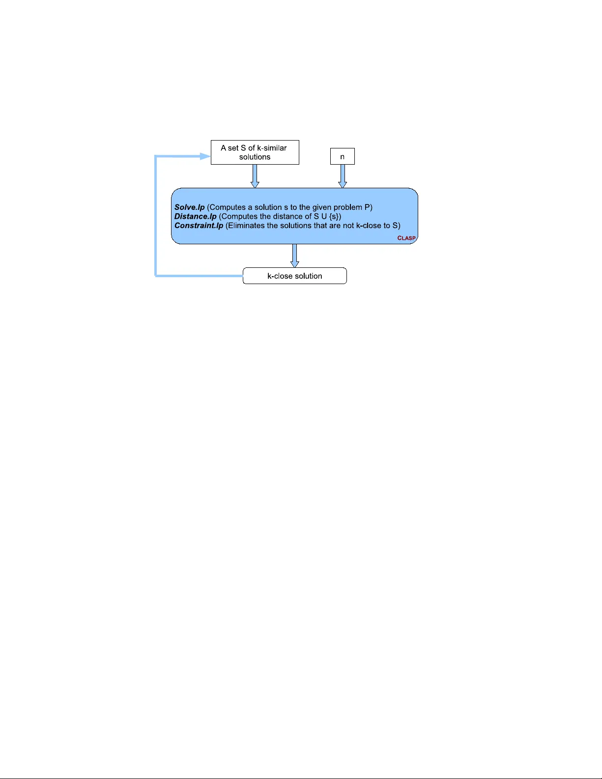
Under consideration for publication in Theory and Practice of Lo gic Pr ogramming 1 F inding Similar/Diverse Solutions in Answer Set Pr ogr amming ∗ THOMAS EITER Institute of Information Systems, V ienna University of T echnology , V ienna, Austria E-mail: eiter@kr .tuwien.ac.at ESRA ERDEM and HALIT ERDOGAN F aculty of Engineering and Natural Sciences, Sabanci University , Istanb ul, T urke y E-mail: { esraer dem,halit } @sabanciuniv .edu MICHAEL FINK Institute of Information Systems, V ienna University of T echnology , V ienna, Austria E-mail: ﬁnk@kr .tuwien.ac.at submitted 11 J anuary 2011; r evised 27 J uly 2011; accepted 11 August 2011 Abstract For some computational problems (e.g., product conﬁguration, planning, diagnosis, query answering, phylogeny reconstruction) computing a set of similar/diverse solutions may be desirable for better decision-making. With this motiv ation, we have studied sev eral decision/optimization versions of this problem in the context of Answer Set Programming (ASP), analyzed their computational comple x- ity , and introduced ofﬂine/online methods to compute similar/diverse solutions of such computational problems with respect to a giv en distance function. All these methods rely on the idea of comput- ing solutions to a problem by means of ﬁnding the answer sets for an ASP program that describes the problem. The ofﬂine methods compute all solutions of a problem in advance using the ASP for- mulation of the problem with an e xisting ASP solv er , like C L A S P , and then identify similar/div erse solutions using some clustering methods (possibly in ASP as well). The online methods compute similar/div erse solutions of a problem following one of the three approaches: by reformulating the ASP representation of the problem to compute similar/div erse solutions at once using an existing ASP solver; by computing similar/diverse solutions iterativ ely (one after other) using an existing ASP solver; by modifying the search algorithm of an ASP solver to compute similar/div erse solu- tions incrementally . All these methods are sound; the ofﬂine method and the ﬁrst online method are complete whereas the others are not. W e ha ve modiﬁed C L A S P to implement the last online method and called it C L A S P - N K . In the ﬁrst two online methods, the given distance function is represented in ASP; in the last one howe ver it is implemented in C++. W e have sho wed the applicability and the effecti v eness of these methods using C L A S P or C L A S P - N K on two sorts of problems with different distance measures: on a real-world problem in phylogenetics (i.e., reconstruction of similar/di verse phylogenies for Indo-European languages), and on several planning problems in a well-known do- main (i.e., Blocks W orld). W e hav e observ ed that in terms of computational ef ﬁciency (both time and space) the last online method outperforms the others; also it allows us to compute similar/diverse ∗ Part of the results in this paper are contained, in preliminary form, in Proceedings of the 25’th International Conference on Logic Programming (ICLP 2009) . This work was partially supported by FWF (Austrian Science Funds) project P20841, the W olfgang Pauli Institute, and TUBIT AK Grants 107E229 and 108E229. 2 Eiter et. al. solutions when the distance function cannot be represented in ASP (e.g., due to some mathematical functions not supported by the ASP solvers) b ut can be easily implemented in C++. KEYWORDS : similar/di verse solutions, answer set programming, similar/di verse phylogenies, sim- ilar/div erse plans 1 Introduction For man y computational problems, the main concern is to ﬁnd a best solution (e.g., a most preferred product conﬁguration, a shortest plan, a most parsimonious phylogeny) with re- spect to some well-described criterion. On the other hand, in many real-world applications, computing a subset of good solutions that are similar/di verse may be desirable for better decision-making. For one reason, the gi ven computational problem may have too man y good solutions, and the user may want to e xamine only a fe w of them to pick one. Also, in many real-world applications the users usually take into account furthermore criterion that are not included in the formulation of the optimization problem; in such cases, good solutions similar to a best one may also be useful. Here are some examples from sev eral domains illustrating the usefulness of ﬁnding similar/div erse solutions. Product conﬁguration Consider , for instance, a variation of the example given in (He- brard et al. 2005) about buying a car . Suppose that there is a product advisor that asks customers about their constraints/preferences about a car , and then lists the av ailable ones that match their constraints/preferences. Howe ver , such a list may be too long. In that case, the customer might ask for a fe w cars that not only suit her constraints/preferences b ut also are as diverse as possible. Then, if she likes one particular car among them, she might ask for other cars that are as similar as possible to this particular car . Also, the customer may hav e other (possibly secondary) criterion that the product advisor has not asked about; and thus the best alternati ves listed by the product advisor may not cov er some of the good possibilities. Then, the user may ask for a couple of good enough conﬁgurations that are distant from a set of best conﬁgurations. Planning Giv en an initial state, goal conditions, and a description of actions, planning is the problem of ﬁnding a sequence of actions (i.e., a plan) that would lead the initial state to a goal state. Planning is applied in various domains, such as robotics, web service com- position, and genome rearrangement. In planning, it may be desirable to compute a set of plans that are similar to each other , so that, when the plan that is being executed fails, one can switch to a most similar one. For instance, consider a variation of the example given in (Sri v astav a et al. 2007) in connection with modeling web service composition as a plan- ning problem (McIlraith and Son 2002): suppose that the web service engine computes a plan/composition; then it can compute a set of compositions similar to this particular one, so that if a f ailure occurs while e xecuting one composition, an alternati ve composition which is less likely to be failing simultaneously can be used (Chaﬂe et al. 2006). Alterna- tiv ely , let us consider planning in the context of robotics in a dynamic environment with uncertainties. If the plan failure is, for instance, due to some collisions with an obstacle as F inding Similar/Diverse Solutions in Answer Set Pr ogramming 3 in the scenarios presented in (Caldiran et al. 2009), the agent may want to ﬁnd a plan that is distant from the pre viously computed plan so that it does not collide with the obstacle again. Phylogeny reconstruction Phylogeny reconstruction is the problem of inferring a leaf- labeled rooted directed tree (i.e., phylogeny) that would characterize the ev olutionary re- lations between a family of species based on their shared traits. Phylogeny reconstruc- tion is important for research areas as disparate as genetics, historical linguistics, zoology , anthropology , archaeology , etc.. For example, a phylogeny of parasites may help zool- ogists to understand the ev olution of human diseases (Brooks and McLennan 1991); a phylogeny of languages may help scientists to better understand human migrations (White and O’Connell 1982). For a given set of taxonomic units, some existing phylogenetic sys- tems, like that of (Brooks et al. 2005; Brooks et al. 2007), generate more than one good phylogeny that e xplains the e volutionary relationships between the gi ven taxonomic units. Howe v er , usually there are too many phylogenies computed by a system, an expert needs to compare these phylogenies in detail, by analyzing the similar/diverse ones with respect to some distance measure, to pick the most plausible ones. Motiv ated by such examples, we have studied v arious problems related to computing similar/div erse solutions in the context of a new declarativ e programming paradigm, called Answer Set Programming (ASP) (Lifschitz 2008). W e have also introduced general of- ﬂine/online methods in ASP that can be applied to v arious domains for such computations. In ASP , a combinatorial search problem is represented as an ASP program whose models (called “answer sets”) correspond to the solutions. The answer sets for the giv en formal- ism can be computed by special systems called answer set solv ers, such as C L A S P (Gebser et al. 2007a). Due to the expressi ve formalism of ASP that allows us to represent, e.g., nega- tion, defaults, aggregates, recursiv e deﬁnitions, and due to the continuous improv ements of efﬁcienc y of solvers, ASP has been used in a wide-range of knowledge-intensi ve appli- cations from dif ferent ﬁelds, such as product conﬁguration (Soininen and Niemel ¨ a 1998), planning (Lifschitz 1999), phylogen y reconstruction (Brooks et al. 2007), de veloping a de- cision support system for a space shuttle (Nogueira et al. 2001), multi-agent planning (Son et al. 2009), answering biomedical queries (Bodenreider et al. 2008). For many of these applications, ﬁnding similar/diverse solutions (and thus the methods we ha ve developed for computing similar/div erse solutions in ASP) could be useful. The main contributions of this paper can be summarized as follo ws. • W e hav e described mainly two kinds of computational problems related to ﬁnding similar/div erse solutions of a given problem, in the context of ASP (Section 3). Both kinds of problems take as input an ASP program P that describes a problem, a distance measure ∆ that maps a set of solutions of the problem to a nonne gativ e integer , and two nonnegati ve integers n and k . One problem asks for a set S of size n that contains k -similar (resp. k -di verse) solutions, i.e., ∆( S ) ≤ k (resp. ∆( S ) ≥ k ); the other problem asks, gi ven a set S of n solutions, for a k -close (resp. k -distant) solution s (resp. s 6∈ S ), i.e., ∆( S ∪ { s } ) ≤ k (resp. ∆( S ∪ { s } ) ≥ k ). Note that, by ﬁxing some parameters and minimizing/maximizing others, we can turn them into various related optimization problems. 4 Eiter et. al. • W e have studied the computational complexity of these decision/optimization prob- lems establishing completeness results under reasonable assumptions for the prob- lem parameters (Section 4). • W e hav e introduced an ofﬂine method to compute a set of n k -similar (resp. k - div erse) solutions to a giv en problem, by computing all solutions in advance using ASP and then ﬁnding similar (resp. di verse) solutions using some clustering meth- ods, possibly in ASP as well (Section 5.1.1). This method is sound and complete, assuming that the ASP formulations are correct. • W e hav e introduced three online methods to compute a set of n k -similar (resp. k -div erse) solutions to a giv en problem (Sections 5.1.2, 5.1.3 and 5.1.4). — Online Method 1 reformulates the giv en program to compute n -distinct solu- tions and formulates the distance function as an ASP program, so that all n k -similar (resp. k -di verse) solutions can be extracted from an answer set for the union of these ASP programs. — Online Method 2 does not modify the ASP program encoding the problem, but formulates the distance function as an ASP program, so that a unique k -close (resp. k -distant) solution can be e xtracted from an answer set for the union of these ASP programs and a previously computed solution; by iterativ ely computing k -close (resp. k -distant) solutions one after other , we can compute online a set of n k -similar (or k -div erse) solutions. — Online Method 3 does not modify the ASP encoding of the problem, and does not formulate the distance function as an ASP program, b ut it modiﬁes the search algorithm of an ASP solver , in our case C L A S P (Gebser et al. 2007b), to compute all n k -similar (or k -div erse) solutions at once. The distance function is implemented in C++; in that sense, Online Method 3 allows for ﬁnding similar/div erse solutions when the distance function cannot be deﬁned in ASP . All the methods are sound, assuming that the ASP formulations are correct. Online Method 1 is complete; howe ver , Online Methods 2 and 3 are not because the com- putation of the similar/diverse solutions depend on the ﬁrst solution computed by C L A S P . • W e have illustrated the applicability of these approaches on two sorts of problems: phylogeny reconstruction (based on the ASP encoding of the problem as in (Brooks et al. 2007)) and planning (based on the ASP encoding of the Blocks W orld as in (Erdem 2002)). — For phylogeny reconstruction, we have deﬁned novel distance measures for a set of phylogenies (Section 6.1), described ho w the ofﬂine method and the on- line methods are applied to ﬁnd similar/di v erse ph ylogenies (Section 6.2), and compared the efﬁcienc y and effecti v eness of these methods on the family of Indo-European languages studied in (Brooks et al. 2007) (Section 6.3). Since there is no phylogenetic system that helps e xperts to analyze phylogenies by comparing them, this particular application of our methods also plays a signif- icant role in phylogenetics. In fact, Ofﬂine Method and Online Method 3 are integrated in the phylogenetics system P H Y L O - A S P (Erdem 2009). F inding Similar/Diverse Solutions in Answer Set Pr ogramming 5 — For planning, we ha ve considered the action-based Hamming distance of (Sri- vasta v a et al. 2007) to measure the distance among plans, and compared the efﬁcienc y and effecti veness of the of ﬂine method and the online methods on some Blocks W orld problems (Section 7). Finding similar/di verse solutions has earlier been studied in the conte xt of propositional logic (Bailleux and Marquis 1999), constraint programming (Hebrard et al. 2005; Hebrard et al. 2007), and automated planning (Sriv astav a et al. 2007). These studies consider the Hamming distance (Hamming 1950) as a measure to compute distances between solutions. Unlike the problems studied in related work, the problems we have studied are not conﬁned to polynomial-time distance functions with polynomial range. A more detailed discussion on related work is presented in Section 8. 2 Answer Set Programming W e study ﬁnding similar/div erse solutions in the context of Answer Set Programming (ASP) (Lifschitz 2008)—a new declarative programming paradigm where the idea is to represent a combinatorial search problem as a “program” whose models (called “answer sets” (Gelfond and Lifschitz 1991)) correspond to the solutions. This is in the v ein of SA T solving, which became popular after a surprising success in the area of planning (Kautz and Selman 1992), but offers in comparison features like variables ranging ov er domain elements, easy deﬁnition of transiti v e closure, and nonmonotonic neg ation. Furthermore, a range of special constructs, such as aggregates, weight constraints and priorities, that are useful in practical applications are supported by v arious ASP solvers; for more discussion, see Section 8. Before we proceed discussing our methods for ﬁnding similar/div erse solutions in ASP , let us present the syntax of the kind of programs considered in this paper , and deﬁne the concept of an answer set for such programs. 1 Pr ogr ams The syntax of formulas, rules and programs is deﬁned as follo ws. Formulas are formed from propositional atoms and 0-place connecti ves > and ⊥ using ne gation (written as not ), conjunction (written as a comma) and disjunction (written as a semicolon). A rule is an expression of the form F ← G (1) where F is an atom or ⊥ , and G is a formula; F is called the head and G is called the body of the rule. A rule of the form F ← > will be identiﬁed with the formula F . A rule of the form ⊥ ← F (called a constraint ) will be abbreviated as ← F . A (normal nested) program is a ﬁnite set of rules. If bodies of all rules in a program are of the form A 1 , . . . , A m , not A m +1 , . . . , not A n 1 Answer sets are deﬁned for programs of a more general form that may contain classical negation ¬ and dis- junction (Gelfond and Lifschitz 1991) and nested expressions (Lifschitz et al. 1999) in heads of rules as well. See (Lifschitz 2010) for deﬁnitions of answer sets. 6 Eiter et. al. then the program is a normal program . A program is positive if it does not contain any negation. Answer Sets T o deﬁne the concept of an answer set for a program, let us ﬁrst deﬁne the satisfaction relation and the reduct of a program. The satisfaction relation X | = F between a set X of atoms and a formula F is deﬁned recursiv ely , as follows: • for an atom A , X | = A if A ∈ X • X | = > • X 6| = ⊥ • X | = ( F , G ) if X | = F and X | = G • X | = ( F ; G ) if X | = F or X | = G • X | = not F if X 6| = F . W e say that X satisﬁes a program Π (symbolically , X | = Π ) if, for ev ery rule F ← G in Π , X | = F whene ver X | = G . The reduct F X of a formula F with respect to a set X of atoms is deﬁned recursi vely , as follows: • if F is an atom or a 0-place connectiv e then F X = F • ( F , G ) X = F X , G X • ( F ; G ) X = F X ; G X • ( not F ) X =  ⊥ , if X | = F , > , otherwise. The reduct Π X of a program Π with respect to X is the set of rules F X ← G X for all rules F ← G in Π . Let us ﬁrst deﬁne the answer set for a program Π that does not contain negation. W e say that X is an answer set for Π , if X is minimal with respect to set inclusion ( ⊆ ) among the sets of atoms that satisfy Π . For instance, the set { p } is the answer set for the program consisting of the single rule p ← · (2) Now consider a program Π that may contain neg ation. A set X of atoms is an answer set for Π if it is the answer set for the reduct Π X . For instance, the reduct of the program p ← not not p (3) relativ e to { p } is (2). Since { p } is the answer set for (2), { p } is an answer set for program (3). Similarly , {} is an answer set for program (3) as well. Repr esenting a Pr oblem in ASP The idea of ASP is to represent a computational problem as a program whose answer sets correspond to the solutions of the problem, and to ﬁnd the answer sets for that program using an answer set solver . When we represent a problem in ASP , two kinds of rules play an important role: those F inding Similar/Diverse Solutions in Answer Set Pr ogramming 7 that “generate” many answer sets corresponding to “possible solutions”, and those that can be used to “eliminate” the answer sets that do not correspond to solutions. Rules (3) are of the former kind: they generate the answer sets { p } and {} . Constraints are of the latter kind. For instance, adding the constraint ← p to program (3) eliminates the answer sets for the program that contain p . In ASP , we use special constructs of the form { A 1 , . . . , A n } c (4) (called choice expressions ), and of the form l ≤ { A 1 , . . . , A m } ≤ u (5) (called cardinality expressions ) where each A i is an atom and l and u are nonnegati ve integers denoting the “lo wer bound” and the “upper bound” (Simons et al. 2002). Programs using these constructs can be viewed as abbreviations for normal nested programs deﬁned abov e, due to (Ferraris and Lifschitz 2005). For instance, the follo wing program { p } c ← stands for program (3). The constraint ← 2 ≤ { p , q , r } stands for the constraints ← p , q ← p , r ← q , r · Expression (4) describes subsets of { A 1 , . . . , A n } . Such expressions can be used in heads of rules to generate many answer sets. F or instance, the answer sets for the program { p , q , r } c ← (6) are arbitrary subsets of { p , q , r } . Expression (5) describes the subsets of the set { A 1 , . . . , A m } whose cardinalities are at least l and at most u . Such expressions can be used in constraints to eliminate some answer sets. For instance, adding the constraint ← 2 ≤ { p , q , r } to program (6) eliminates the answer sets for (6) whose cardinalities are at least 2. Adding the constraint ← not (1 ≤ { p , q , r } ) (7) to program (6) eliminates the answer sets for (6) whose cardinalities are not at least 1. W e abbreviate the rules { A 1 , . . . , A m } c ← Body ← not ( l ≤ { A 1 , . . . , A m } ) ← not ( { A 1 , . . . , A m } ≤ u ) 8 Eiter et. al. by l ≤ { A 1 , . . . , A m } c ≤ u ← Body · For instance, rules (6), (7) and ← not ( { p , q , r } ≤ 1) can be written as 1 ≤ { p , q , r } c ≤ 1 ← whose answer sets are the singleton subsets of { p , q , r } . F inding a Solution using an Answer Set Solver Once we represent a computational prob- lem as a program whose answer sets correspond to solutions of the problem, we can use an answer set solver to compute the solutions of the problem. T o present a program to an answer set solver , like C L A S P , we need to make some syntactic modiﬁcations. The syntax of the input language of C L A S P is more limited in some ways than the class of programs deﬁned abov e, but it includes many useful special cases. For instance, the head of a rule can be an expression of one of the forms { A 1 , . . . , A n } c l ≤ { A 1 , . . . , A n } c { A 1 , . . . , A n } c ≤ u l ≤ { A 1 , . . . , A n } c ≤ u but the superscript c and the sign ≤ are dropped. The body can contain cardinality expres- sions but the sign ≤ is dropped. In the input language of C L A S P , :- stands for ← , and each rule is followed by a period. A group of rules that follow a pattern can be often described in a compact way using “(schematic) variables”. V ariables must be capitalized. For instance, the program Π n p i ← not p i +1 (1 ≤ i ≤ n ) can be presented to C L A S P as follows: index(1..n). p(I) :- not p(I+1), index(I). Here index is a “domain predicate” used to describe the range of variable I . V ariables can be also used “locally” to describe the list of formulas in a cardinality expression. F or instance, the rule 1 ≤ { p 1 , . . . , p n } ≤ 1 can be expressed in C L A S P as follows index(1..n). 1{p(I) : index(I)}1. C L A S P ﬁnds an answer set for a program in two stages: ﬁrst it gets rid of the schematic variables using a “grounder”, like G R I N G O , and then it ﬁnds an answer set for the ground program using a DPLL-like branch and bound algorithm (outlined in Algorithm 2). F inding Similar/Diverse Solutions in Answer Set Pr ogramming 9 3 Computational Problems W e study various problems related to ﬁnding similar/div erse solutions to a computational problem P formulated in ASP . For that, we assume that the problem is represented as a normal (possibly nested) program P whose answer sets characterize solutions of the problem. More precisely , let S ol ( P ) denote the set of solutions of P and let AS ( P ) denote the set of answer sets of P . Then, there is a man y-to-one mapping of AS ( P ) onto S ol ( P ) . Moreov er , giv en an answer set of P the corresponding solution from S ol ( P ) can efﬁciently be extracted. W e also assume that a distance function that maps a set S of solutions to a number is deﬁned, to measure how similar/div erse the solutions are in S . T o this end, we consider set-distance measures ∆ : 2 S ol ( P ) 7→ N 0 on solutions for P . W e are mainly interested in two sorts of problems related to computation of a div erse/similar collection of solutions: n k - S I M I L A R S O L U T I O N S (resp. n k - D I V E R S E S O L U T I O N S ) Giv en an ASP program P that formulates a computational problem P , a distance measure ∆ that maps a set of solutions for P to a nonnegativ e integer , and two nonnegati v e integers n and k , decide whether a set S of n solutions for P exists such that ∆( S ) ≤ k (resp. ∆( S ) ≥ k ). k - C L O S E S O L U T I O N (resp. k - D I S TA N T S O L U T I O N ) Giv en an ASP program P that formulates a computational problem P , a distance measure ∆ that maps a set of solutions for P to a nonnegati ve integer , a set S of solutions for P , and a nonne gati ve integer k , decide whether some solution s ( s 6∈ S ) for P exists such that ∆( S ∪ { s } ) ≤ k (resp. ∆( S ∪ { s } ) ≥ k ). For instance, suppose that the ASP program P describes the phylogen y reconstruction problem for Indo-European languages as in (Brooks et al. 2005); so each answer set of P represents a phylogeny for Indo-European languages. Using this ASP program with an existing ASP solver , one can compute many phylogenies for the same input dataset and with the same input parameters. Instead of analyzing all of these phylogenies manually , a historical linguist may ask for , for instance, three phylogenies whose div ersity is at least 20 with respect to some domain-independent or domain-dependent distance function ∆ ; this problem is an instance of n k -diverse solutions problem where n = 3 and k = 20 . On the other hand, a historical linguist may hav e found two phylogenies P 1 and P 2 that are plausible, for instance, based on some archeological evidence, and she may want to infer a similar phylogen y whose distance from { P 1 , P 2 } is at most 10; this problem is an instance of k -close solution problem where k = 10 . The ﬁrst kind of problems abov e has tw o parameters, n and k , so we can ﬁx one and try to minimize (resp. maximize) the distance between solutions to ﬁnd the most similar (resp. div erse) solutions. n M O S T S I M I L A R S O L U T I O N S (resp. n M O S T D I V E R S E S O L U T I O N S ) Giv en an ASP program P that formulates a computational problem P , a distance measure ∆ that maps a set of solutions for P to a nonnegati ve integer , and a nonneg- ativ e integer n , ﬁnd a set S of n solutions for P with the minimum (resp. maximum) distance ∆( S ) . M A X I M A L n k - S I M I L A R S O L U T I O N S (resp. M A X I M A L n k - D I V E R S E S O L U T I O N S ) 10 Eiter et. al. Giv en an ASP program P that formulates a computational problem P , a distance measure ∆ that maps a set of solutions for P to a nonnegati ve integer , and a non- negati v e integer k , ﬁnd a ⊆ -maximal set S of at most n solutions for P such that ∆( S ) ≤ k (resp. ∆( S ) ≥ k ) exists. In the second class of problems, we can try to minimize (resp. maximize) the distance k between a solution and a set of solutions, to ﬁnd the closest (resp. most distant) solution. C L O S E S T S O L U T I O N (resp. M O S T D I S TA N T S O L U T I O N ) Giv en an ASP program P that formulates a computational problem P , a distance measure ∆ that maps a set of solutions for P to a nonne gati ve inte ger , and a set S of solutions for P , ﬁnd a solution s ( s 6∈ S ) for P with the minimum (resp. maximum) distance ∆( S ∪ { s } ) . W e can generalize k - C L O S E S O L U T I O N (resp. k - D I S TA N T S O L U T I O N ) problems to sets of solutions: k - C L O S E S E T (resp. k - D I S TA N T S E T ) Giv en an ASP program P that formulates a computational problem P , a distance measure ∆ that maps a set of solutions for P to a nonnegati ve integer , a set S of solutions for P , and a nonnegati ve integer k , decide whether a set S 0 of solutions for P ( S 0 6 = S ) exists such that | ∆( S ) − ∆( S 0 ) | ≤ k (resp. | ∆( S ) − ∆( S 0 ) | ≥ k ). Usually an expert is interested in several kinds of problems to be able to systematically analyze solutions. For instance, a historical linguist may want to ﬁnd three most div erse phylogenies; and after identifying one particular plausible phylogeny among them, she may want to compute another phylogeny that is the closest. An example of such an analysis is shown in Section 6.3 for understanding the classiﬁcation of Indo-European languages. W e note that the problems on similar/di verse solutions from above can be analogously deﬁned for computation problems with multiple (or possibly none) solutions in general, and in particular for such problems with NP complexity . Since ASP can express all NP search problems (Marek and Remmel 2003), in fact similar/diverse solution computation for each such problem can be formulated in the frame work abo ve (in f act with polynomial ov erhead). 4 Complexity Results Before we discuss how the computational problems described in the previous section can be solv ed in ASP , let us turn our attention to the computational complexity of the problems presented in Section 3. In order to do so, we ﬁrst make some reasonable assumptions on some of the problem parameters. In the following we assume that giv en an answer set s of P , extracting a solution of P from s can be accomplished in time polynomial wrt. the size of s . Moreover , w .l.o.g. we identify s with the solution it encodes, and sets S ⊆ S ol ( P ) with corresponding sets of answer sets from AS ( P ) . W e assume that all numbers are gi v en in binary and that the gi ven number n of different solutions to consider (respectiv ely the size of the set S ) for instances of the problems n F inding Similar/Diverse Solutions in Answer Set Pr ogramming 11 T able 1. Complexity results for computing similar solutions. # Problem Complexity 1 n k - S I M I L A R S O L U T I O N S NP 2 k - C L O S E S O L U T I O N NP 3 M A X I M A L n k - S I M I L A R S O L U T I O N S FNP / / log 4 n M O S T S I M I L A R S O L U T I O N S FP NP ( FNP / / log ) 5 C L O S E S T S O L U T I O N FP NP ( FNP / / log ) 6 k - C L O S E S E T NP k - S I M I L A R S O L U T I O N S , M A X I M A L n k - S I M I L A R S O L U T I O N S , and n M O S T S I M I L A R S O L U T I O N S is polynomial in the size of the input. The same assumption applies to the size of the sets S 0 to consider in instances of k - C L O S E S E T problems. Furthermore, we consider distance measures ∆ such that deciding whether ∆( S ) ≤ k (resp. whether ∆( S ) ≥ k ) for a gi ven k is in NP . Moreov er , we assume that the value of ∆( S ) is bounded by an exponential in the size of S (and thus has polynomially many bits in the size of S ). Thus, when considering ∆ as an input to a problem, we assume that it is given as the description of a non-deterministic T uring machine M ≤ ∆ , or M ≥ ∆ , or both, where M ≤ ∆ (resp. M ≥ ∆ ) nondeterministically decides ∆( S ) ≤ k (resp. ∆( S ) ≥ k ) in time polynomial in the length of its input S and k . Consequently , a witness for a computation of M χ ∆ on some input S and k , where χ ∈ {≤ , ≥} is a sequence of conﬁgurations of M χ ∆ , such that the input tape contains S and k in the initial conﬁguration, successi ve conﬁgurations correspond to transitions of M χ ∆ , and the ﬁnal conﬁguration accepts. In addition, we say that a ∆ is normal if | S | ≤ 1 implies ∆( S ) = 0 . Under these assumptions, the computational complexity (cf. (Papadimitriou 1994) for a background on the subject) of the problems concerning the computation of similar/di v erse solutions we are interested in, is gi ven in T able 1. All entries are completeness results (under usual reductions) and hardness holds e ven if ∆( S ) is computable in polynomial time. Moreo ver , the results are the same for the ‘symmetric’ problems, i.e., when S I M I L A R is replaced with D I V E R S E , and C L O S E is replaced with D I S TA N T , respectiv ely . The proofs are included in Appendix A. Theor em 1 Problem n k - S I M I L A R S O L U T I O N S (resp. n k - D I V E R S E S O L U T I O N S ) is NP -complete. Hardness holds ev en if ∆( S ) is computable in constant time and for an y normal ∆ . Membership for problem n k - S I M I L A R S O L U T I O N S (resp. n k - D I V E R S E S O L U T I O N S ) follows from the fact that we can guess not only a candidate set S via the program P (since S is polynomially bounded) b ut also a witness for ∆( S ) ≤ k (resp. ∆( S ) ≥ k ), and check in polynomial time whether e very s ∈ S is a solution and that ∆( S ) ≤ k (resp. ∆( S ) ≥ k ). For hardness, one simply reduces answer -set e xistence for normal, propositional programs to this problem, which is an NP -complete problem. For a hardness result resorting to partial Hamming distance, one can confer (Bailleux and Marquis 1999). In our experiments with phylogeny reconstruction, by Theorem 1, we know that deciding the existence of n k -similar (resp. k -di verse) phylogenies is NP -complete, if the distance 12 Eiter et. al. measure is the nearest neighbor interchange distance (DasGupta et al. 1997) whose com- putation is beyond polynomial time, or if the distance measure is the nodal distance or comparison of descendants distance (both deﬁned in Section 6.1) that are computable in polynomial time. Also, in planning, if we consider the Hamming distance (Hamming 1950) (as deﬁned in Section 7), which is polynomially computable, or the edit distance inv olving transpositions, which is conjectured to be NP-hard (Bafna and Pevzner 1998), deciding the existence of n k -similar (resp. k -div erse) plans is NP -complete. Therefore, it mak es sense to ﬁnd similar/div erse phylogenies/plans using ASP . By similar arguments we obtain NP -completeness for problem k - C L O S E S O L U T I O N (resp. k - D I S TA N T S O L U T I O N ). Theor em 2 Problem k - C L O S E S O L U T I O N (resp. k - D I S TA N T S O L U T I O N ) is NP -complete. Hardness holds ev en if ∆( S ) is computable in constant time and for an y normal ∆ . When looking for maximal sets of solutions, we face a function problem; here we also assume a polynomial upper bound on the size of the sets S to consider (giv en by input n and our corresponding assumption). Recall that function problems generalize decision problems asking for a ﬁnite, possibly empty set of solutions of every problem instance. The solutions to function problems can be computed by transducers, i.e., possibly nonde- terministic T uring machines equipped with an output tape, which contains a solution if the input is accepted. Note that if the T uring machine is nondeterministic, then it computes a multi-v alued (partial) function. For instance, FNP is the class of multi-valued function problems that can be solv ed by a nondeterministic transducer in polynomial time, such that a giv en solution candidate can be checked in polynomial time. In particular , M A X I M A L n k - S I M I L A R S O L U T I O N S (resp. n M A X I M A L k - D I V E R S E S O - L U T I O N S ) is solv able in FNP / / log . Intuitiv ely , FNP / / log is the class of function problems solvable in polynomial time using a nondeterministic T uring machine with output tape that may consult once an oracle that computes the optimal value of an optimization problem whose associated decision problem is solvable in NP , provided that this value has loga- rithmically many bits in the size of the input (see, e.g., (Chen and T oda 1995; Eiter and Subrahmanian 1999) for more information on FNP / / log and other function classes used in this section). Theor em 3 Problem M A X I M A L n k - S I M I L A R S O L U T I O N S (resp. M A X I M A L n k - D I V E R S E S O L U - T I O N S ) is FNP / / log -complete. Hardness holds e ven if ∆( S ) is computable in polynomial time. Membership can be shown by computing the maximum cardinality of a set of at most n solutions S using the oracle. Obviously , computing the maximum cardinality c of a set of at most n solutions S is an optimization problem whose associated decision problem is the following: decide whether a giv en c (such that c ≤ n ) is the cardinality of a set S of (at most n ) solutions. Since the latter problem is in NP (guess S and check in polynomial time whether | S | = c , ∆( S ) ≤ k , and e very s ∈ S is a solution), the optimization problem is amenable to the oracle provided that the computed v alue (optimal c ) has log arithmically many bits in the size of the input. Note that since | S | is polynomially bounded in the size of F inding Similar/Diverse Solutions in Answer Set Pr ogramming 13 the input, it has log arithmically man y bits as required. Once the optimal v alue is computed, one can nondeterministically compute a set S of respecti ve size together with a witness for ∆( S ) ≤ k , and check in polynomial time that this is indeed the case. Hardness can be shown by a reduction of X -MinModel (cf. (Chen and T oda 1995)). W e remark that the slightly different problem asking for a polynomial-size set S of solutions such that ∆( S ) is minimal (respectively maximal), again under the assumption that this value has logarithmically many bits, is also FNP / / log -complete. For this variant, hardness can be sho wn, e.g., for ∆( S ) that takes the minimal (respecti vely maximal) Hamming dis- tance between answer sets in S on a subset of the atoms; note that such a partial Hamming distance is a natural measure for problem encodings, where the disagreement on output atoms is measured. Theor em 4 Problem n M O S T S I M I L A R S O L U T I O N S (resp. n M O S T D I V E R S E S O L U T I O N S ) is FP NP - complete, and FNP / / log -complete if the v alue of ∆( S ) is polynomial in the size of S . Hardness holds ev en if ∆( S ) is computable in polynomial time. FP NP -membership of n M O S T S I M I L A R S O L U T I O N S (resp. n M O S T D I V E R S E S O L U - T I O N S ) is obtained by ﬁrst using the NP -oracle to compute the minimum distance using binary search (deciding polynomially many n k - S I M I L A R S O L U T I O N S problems). Then, the oracle is used to compute some suitable S in polynomial time. Hardness follows from a reduction of the Tra veling Salesman Problem (TSP). Notably , if the distances are poly- nomial in the size of the input, i.e., if the value of ∆( S ) is polynomially bounded in the size of S , then the problem is FNP / / log -complete. Proceeding similarly as before, completeness for FP NP (resp. FNP / / log if ∆( S ) is small) is obtained for C L O S E S T S O L U T I O N (and for M O S T D I S TA N T S O L U T I O N ): Theor em 5 Problem C L O S E S T S O L U T I O N (resp. M O S T D I S TA N T S O L U T I O N ) is FP NP -complete, and FNP / / log -complete if the value of ∆( S ) is polynomial in the size of S . Hardness holds ev en if ∆( S ) is computable in polynomial time. For the generalization of k - C L O S E S O L U T I O N (resp. of k - D I S TA N T S O L U T I O N ) to sets, namely k - C L O S E S E T (resp. k - D I S TA N T S E T ), NP -completeness holds by similar argu- ments as for the former problem(s): Theor em 6 Problem k - C L O S E S E T (resp. k - D I S TA N T S E T ) is NP -complete. Hardness holds e ven if ∆( S ) is computable in constant time and for any normal ∆ . Discussion The results above, summarized in T able 1, show that computing similar solu- tions is intractable in general. This already holds under the reasonable assumption that the distance measure ∆ is normal, where all considered decision problems are NP -complete. The precise complexity characterization of the search problems ( M A X I M A L n k - S I M I L A R S O L U T I O N S , n M O S T S I M I L A R S O L U T I O N S , and C L O S E S T S O L U T I O N ) rev eals some in- formation about the type of algorithm we can expect to be suitable for solving these prob- lems in practice (for background, see (Chen and T oda 1995) and references therein). In 14 Eiter et. al. particular , we may not expect that they can be solved by parallelization to NP -problems in polynomial time, i.e., solve in parallel polynomially many NP -problems, e.g., SA T in- stances, and then combine the results. On the other hand, for problem M A X I M A L n k - S I M I L A R S O L U T I O N S this is possible under randomization, i.e., with high probability of a correct outcome, due to the characteristics of FNP / / log , while this is not the case for the problems n M O S T S I M I L A R S O L U T I O N S and C L O S E S T S O L U T I O N in the general case. Rather , the results suggest that consecutiv e, dependent calls to NP oracles are needed. In- tuitiv ely , backtracking-style algorithms, which explore the search space to ﬁnd solutions and then see to (dis)pro ve optimality by ﬁnding better solutions, appropriately reﬂect adap- tivity . Howe v er , from a worst-case complexity perspectiv e, a simple realization of such a scheme may not be optimal, as far too many solution improvements (exponentially resp. polyno- mially many under “small” distance values) may happen until an optimal solution is found; here a two phase algorithm (ﬁrst compute the optimal solution cost in binary search and then a solution of that cost, e.g., with backtracking) gives better guarantees. In practice, one may intertwine bound and solution computation and conduct a binary search ov er computations of solutions within a giv en bound. In the next section, we consider ﬁrst solving the search problem analog of the decision problem n k S I M I L A R S O L U T I O N S , using different approaches, ranging from declarativ e encodings in ASP ov er the explicit respecti vely implicit set of solutions, to a generalized backtracking algorithm for e v aluation ASP programs. W e then consider solving the related search problems n M O S T S I M I L A R S O L U T I O N S and M A X I M A L n k - S I M I L A R S O L U T I O N S based on the above considerations. Finally , we discuss how we can solve the problems k - C L O S E S O L U T I O N , C L O S E S T S O L U T I O N and k - C L O S E S E T utilizing the methods intro- duced for n k S I M I L A R S O L U T I O N S and its variants. 5 Computing Similar/Diverse Solutions Now we have a better understanding of the computational problems, let us present our com- putational methods to ﬁnd n k -similar/div erse solutions, n most similar/div erse solutions and maximal n k -similar/di verse solutions for a gi ven computational problem P . Since the computation of similar solutions and di v erse solutions are symmetric, for simplicity , let us only focus on the problems related to similarity . In the follo wing, suppose that the problem P is described by an ASP program Solve.lp . 5.1 Computing n k -Similar Solutions T o compute a set of n solutions whose distance is at most k , we introduce an ofﬂine method and three online methods. 5.1.1 Ofﬂine Method In the ofﬂine method, we compute the set S of all the solutions for P in advance using the ASP program Solve.lp , with an existing ASP solver . Then, we use some clustering F inding Similar/Diverse Solutions in Answer Set Pr ogramming 15 Algorithm 1 Ofﬂine Method Input: A set S of solutions, a distance function d : S × S 7→ N , and two nonnegati v e integers n and k . Output: A set C of n solutions whose distance is at most k . V ← Deﬁne a set of | S | vertices, each denoting a unique solution in S ; E = {{ v i , v j } | v i 6 = v j , v i , v j denote s i , s j ∈ S , d ( s i , s j ) ≤ k } ; C ← Find a clique of size n in h V , E i ; retur n C method to ﬁnd similar solutions in S . The idea is to form clusters of n solutions, measure the distance of each cluster , and pick the cluster whose distance is less than or equal to k . W e can compute clusters of n solutions whose distance is at most k by means of a graph problem: build a complete graph G whose nodes correspond to the solutions in S and edges are labeled by distances between the corresponding solutions; and decide whether there is a clique C of size n in G whose weight (i.e., the distance of the set of solutions denoted by the weight of the clique) is less than or equal to k . The set of vertices in the clique represents n k -similar solutions. The weight of a clique (or the distance ∆ of the solutions in the cluster) can be computed as follows: Giv en a function d to measure the distance between two solutions, let ∆( S ) be the maximum distance between any two solutions in S . Then n k -similar solutions can be computed by Algorithm 1 where the graph G is built as follows: nodes correspond to solutions in S , and there is an edge between two nodes s 1 and s 2 in G if d ( s 1 , s 2 ) ≤ k . Nodes of a clique of size n in this graph correspond to n k -similar solutions. Such a clique can be computed using the ASP formulation in (Lifschitz 2008), or one of the existing exact/approximate algorithms discussed in (Gutin 2003). 5.1.2 Online Method 1: Reformulation Instead of computing all the solutions in advance as in the ofﬂine method, we can com- pute n k -similar solutions to the given problem P on the ﬂy . First we reformulate the ASP program Solve.lp in such a way to compute n -distinct solutions; let us call the reformulation as SolveN.lp . Such a reformulation can be obtained from Solve.lp as follows: 1. W e specify the number of solutions: solution(1..n). 2. In each rule of the program Solve.lp , we replace each atom p(T1,T2,...,Tm) (except the ones specifying the input) with p(N,T1,T2...,Tm) , and add to the body solution(N) . 3. Now we ha ve a program that computes n solutions. T o ensure that they are distinct, we add a constraint which expresses that ev ery two solutions among these n solu- tions are different from each other . Next we describe the distance function ∆ as an ASP program, Distance.lp . In addi- tion, we represent the constraints on the distance function (e.g., the distance of the solutions in S is at most k ) as an ASP program Constraint.lp . Then we can compute n -distinct solutions for the giv en problem P that are k -similar , by one call of an existing ASP solv er 16 Eiter et. al. Fig. 1. Computing n k -similar solutions, with Online Method 1. with the program SolveN.lp ∪ Distance.lp ∪ Constraint.lp , as shown in Fig. 1. Let us giv e an example to illustrate Online Method 1. Example 1 Suppose that we want to compute n k -similar cliques in a graph. Assume that the similarity of two cliques is measured by the Hamming Distance: the distance between tw o cliques C and C 0 is equal to the number of different vertices, ( C \ C 0 ) ∪ ( C 0 \ C ) . The distance of a set S of cliques can be deﬁned as the maximum distance among any tw o cliques in S . The clique problem can be represented in ASP ( Solve.lp ) as in (Lifschitz 2008), also shown in Appendix B (Fig. B 1). The reformulation ( SolveN.lp ) of this ASP program as described abov e can be seen in Fig. B 2 of Appendix B. This reformulation computes n distinct cliques. The Hamming Distance between any two cliques can be represented by the ASP program ( Distance.lp ) shown in Fig. B 3 of Appendix B. Finally , Fig. B 4 shows the constraint ( Constraint.lp ) that eliminates the sets whose distance is abov e k . An answer set for the union of these three programs, SolveN.lp ∪ Distance.lp ∪ Constraint.lp , corresponds to n k -similar cliques. 5.1.3 Online Method 2: Iterative Computation This method does not modify the giv en ASP program Solve.lp as in Online Method 1, but still formulates the distance function and the distance constraints as ASP programs. The idea is to ﬁnd similar/diverse solutions iterativ ely , where the i ’th solution is k -close to the previously computed i − 1 solutions (Fig. 2). Here n iterations lead to n solutions whose distance is at most k (i.e., n k -similar solutions). Note that, lik e Ofﬂine Method and Online Method 1, this method is sound; ho we ver , unlike Ofﬂine Method and Online Method 1, it is not complete since computation of each solution depends on the previously computed solutions. The method may not return n k - F inding Similar/Diverse Solutions in Answer Set Pr ogramming 17 Fig. 2. Computing n k -similar solutions, with Online Method 2. Initially S = ∅ . In each run, a solution is computed and added to S , until | S | = n . The distance function and the constraints in the program ensures that when we add the computed solution to S , the set stays k -similar . similar solutions (e ven it exists) if the pre viously computed solutions comprise a bad solu- tion set. 5.1.4 Online Method 3: Incr emental Computation This method is different from the other two online methods in that it does not modify the ASP program Solve.lp describing the given computational problem P , it does not formulate the distance function ∆ and the distance constraints as ASP programs. Instead, modiﬁes the search algorithm of an existing ASP solver in such a way that the modiﬁed ASP solver can compute n k -similar solutions (Fig. 3). In this method, we modify the search algorithm of the ASP solver C L A S P (V ersion 1.1.3); the modiﬁed version is called C L A S P - N K . The gi ven distance measure ∆ is implemented as a C++ program. Let us describe how we modiﬁed C L A S P to obtain C L A S P - N K . C L A S P performs a DPLL- like (Da vis et al. 1962; Marques-Silv a and Sakallah 1999) branch and bound search to ﬁnd an answer set for a giv en ASP program (Algorithm 2): at each lev el, it “propagates” some literals to be included in the answer set, “selects” new literals to branch on, or “back- tracks” to an earlier appropriate point in search while “learning conﬂicts” to avoid redun- dant search. W e modify C L A S P ’ s algorithm as sho wn in Algorithm 3 to obtain C L A S P - N K : the under - lined parts show these modiﬁcations. T o use C L A S P - N K , one needs to prepare an options ﬁle, NK options , to describe the input parameters to compute n k -similar phylogenies, such as the values n and k , along with the names of predicates that characterize solutions and that are considered for computing the distance between solutions. Note that since an an- swer set (thus a solution) is computed incrementally in C L A S P - N K , we cannot compute the distance between a partial solution and a set of solutions with respect to the gi ven distance function ∆ . Instead, one needs to implement a heuristic function to estimate a lo wer bound 18 Eiter et. al. Fig. 3. Computing n k -similar solutions, with Online Method 3. C L A S P - N K is a modiﬁca- tion of the ASP solv er C L A S P , that tak es into account the distance function and constraints while computing an answer set in such a way that C L A S P - N K becomes biased to compute similar solutions. Each computed solution is stored by C L A S P - N K until a set of n k -similar solutions is computed. Algorithm 2 CLASP Input: An ASP program Π Output: An answer set A for Π A ← ∅ // current assignment of literals 5 ← ∅ // set of conﬂicts while No Answer Set Found do P R O P AG A T I O N ( Π , A , 5 ) // propagate literals if There is a conﬂict in the current assignment then R E S O LV E - C O N FL I C T ( Π , A , 5 ) // learn and update conﬂicts, and backtrack else if Current assignment does not yield an answer set then S E L E C T ( Π , A , 5 ) // select a literal to continue search else retur n A end if end if end while for the distance between any completion s of a partial solution with a set S of pre viously computed solutions. If this heuristic function is admissible then it does not underestimate the distance of S ∪ { s } (i.e., it returns a lower bound that is less than or equal to the optimal lower bound for the distance). Note that similar to Online Method 2, this method is also sound but not complete since each solution depends on all previously computed solutions. F inding Similar/Diverse Solutions in Answer Set Pr ogramming 19 Algorithm 3 CLASP-NK Input: An ASP program Π , nonnegati v e integers n , and k Output: A set X of n solutions that are k similar ( n k -similar solutions) A ← ∅ // current assignment of literals 5 ← ∅ // set of conﬂicts X ← ∅ // computed solutions while | X | < n do P artialSolution ← A L owerBound ← D I S TA N C E - A N A L Y Z E ( X , P artialSolution ) // compute a lower bound for the distance between any completion of a partial solution and the set of previously computed solutions P R O P AG A T I O N ( Π , A , 5 ) // propagate literals if Conﬂict in propagation O R L owerBound > k then R E S O LV E - C O N FL I C T ( Π , A , 5 ) // learn and update conﬂicts, and backtrack else if Current assignment does not yield an answer set then S E L E C T ( Π , A , 5 ) // select a literal to continue search else X ← X ∪ { A } A ← ∅ end if end if end while retur n X 5.2 Computing n Most Similar Solutions In the previous sections, we hav e described some computational methods to solve the decision problem n k - S I M I L A R S O L U T I O N S . Let us discuss how we can solve the opti- mization problem n M O S T S I M I L A R S O L U T I O N S . Let NKSimilar ( n , k ) be a function that returns—with one of the methods described in the previous subsections—a set S of n so- lutions which is k -similar; or returns empty set if no such set exists. Using this function, we can ﬁnd n most similar solutions as follo ws: First we compute a lo wer bound and an upper bound for the distance k of a set of n solutions. Then, we perform a binary search within these bounds to ﬁnd a set S of solutions with the optimal v alue for k . Computations of a lower bound and an upper bound are usually speciﬁc to the particular problem. For instance, consider the clique problem described in Section 5.1.2. W e can ﬁnd two most similar cliques in a graph, specifying the lower bound as 0 and the upper bound as the number of vertices in the graph and using one of the methods described abo ve. 5.3 Computing Maximal n k -Similar Solutions Another optimization problem we are interested in is M A X I M A L n k - S I M I L A R S O L U - T I O N S , which asks for a maximal set of solutions whose distance is at most k . W e can solve this problem by modifying Online Method 2: start with a solution (computed using 20 Eiter et. al. Solve.lp ), then repeatedly ﬁnd a solution which is k -close to the previously found so- lutions until there does not exists such a solution. Recall that Online Method 2 iterates n times; here the iterations continue until no k -close solution is found. Since Online Method 2 is incomplete, this method of computing maximal n k -similar solutions is incomplete as well. 5.4 Computing Close/Distant Solutions W e can solve the problem k - C L O S E S O L U T I O N utilizing the methods for n k - S I M I L A R S O L U T I O N S . F or instance, we can modify Online Method 2: start with a set S of solutions, then ﬁnd a solution which is k -close to S . Based on this modiﬁed method, we can solve the problem C L O S E S T S O L U T I O N : we can compute a lo wer bound and an upper bound for k , and ﬁnd the optimal value for k by a binary search between these bounds as described in the method for n M O S T S I M I L A R S O L U T I O N S . Alternativ ely , for k - C L O S E S O L U T I O N , we can modify the ASP program P ( Solve.lp ) that describes the computational problem P , by adding constraints, to ensure that the an- swer sets for P characterize solutions for P except for the ones included in the giv en set S of solutions. Let us call the modiﬁed ASP program P 0 . Next, we deﬁne a distance mea- sure ∆ 0 that maps a set of solutions for P to a nonnegati v e integer , in terms of the given measure ∆ as follows: ∆ 0 ( X ) = ∆( S ∪ X ) . Then, we can use one of the computational methods introduced for n k - S I M I L A R S O L U T I O N S with the ASP program P 0 , the distance function ∆ 0 and n = 1 . In a similar way , we can ﬁnd a solution to the problem C L O S E S T S O L U T I O N utilizing the computational method for n M O S T S I M I L A R S O L U T I O N S , with the ASP program P 0 , the distance measure ∆ 0 and n = 1 . W e can solve the problem k - C L O S E S E T using one of the computational methods for n k - S I M I L A R S O L U T I O N S as well. For instance, we can use Online Method 1 with n = 1 , 2 , 3 , . . . , m , where m is an upper bound on the number of solutions for P , until a k - close set S 0 of solutions is computed. For each n , we reformulate the ASP program P to compute a set S 0 of n solutions and add a constraint to this reformulation to ensure that S 0 6 = S when n = | S | ; let us call this modiﬁed reformulation P n . Then we try to ﬁnd a k -close set S 0 of n solutions with the ASP program P n , and the distance measure ∆ 00 = | ∆( S ) − ∆( S 0 ) | . Alternativ ely , we can use Online Method 2 or 3 with the ASP program P , with the distance measure ∆ 000 =  ∞ S = S 0 | ∆( S ) − ∆( S 0 ) | otherwise and with n = 1 , 2 , 3 , . . . , m where m is an upper bound on the number of solutions for P . 6 Computing Similar/Diverse Ph ylogenies Let us no w illustrate the usefulness of our methods in a real-world application: reconstruc- tion of e volutionary trees (or phylogenies) of a set of species based on their shared traits. This problem is important for research areas as disparate as genetics, historical linguistics, zoology , anthropology , archeology , etc.. For example, a phylogen y of parasites may help zoologists to understand the e v olution of human diseases (Brooks and McLennan 1991); a F inding Similar/Diverse Solutions in Answer Set Pr ogramming 21 phylogeny of languages may help scientists to better understand human migrations (White and O’Connell 1982). There are sev eral software systems, such as P H Y L I P (Felsenstein 2009), PAU P (Swof- ford 2003) or P H Y L O - A S P (Erdem 2009), that can reconstruct a phylogeny for a set of taxonomic units, based on “maximum parsimony” (Edwards and Cav alli-Sforza 1964) or “maximum compatibility” (Camin and Sokal 1965) criterion. W ith some of these systems, such as P H Y L O - A S P , we can compute many good phylogenies (most parsimonious phy- logenies, perfect phylogenies, phylogenies with most number of compatible traits, etc.) according to the phylogeny reconstruction criterion. In such cases, in order to decide the most “plausible” ones, domain experts manually analyze these phylogenies, since there is no av ailable phylogenetic system that can analyze/compare these phylogenies. For instance, P H Y L O - A S P computes 45 plausible phylogenies for the Indo-European languages based on the dataset of (Brooks et al. 2007). In order to pick the most plausible phylogenies, in (Brooks et al. 2007), the historical linguist Don Ringe analyzes these phy- logenies by trying to cluster these phylogenies into di v erse groups, each containing similar phylogenies. In such a case, ha ving a tool that reconstructs similar/di verse solutions would be useful: with such a tool, an e xpert can compute (instead of computing all solutions) fe w most di v erse solutions, pick the most plausible one, and then compute ph ylogenies that are close to this phylogeny . Let us sho w how our methods can be used for this purpose. Before that, we deﬁne a phylogeny and some distance functions to measure the similarity/di v ersity of phylogenies. 6.1 Distance Measures for Phylogenies A phylogeny for a set of taxa is a ﬁnite rooted leaf-labeled binary directed tree h V , E i with a set L of lea ves ( L ⊆ V ). The set L represents the given taxonomic units, whereas the set V describes their ancestral units and the set E describes the genetic relationships between them. The labelings of leav es denote the v alues of shared traits at those nodes. W e consider distance measures that depend on topologies of phylogenies, therefore, while deﬁning them we discard these labelings. There are v arious measures to compute the distance between two phylogenies (Nye et al. 2006; Robinson and Foulds 1981; Hon et al. 2000; Kuhner and Felsenstein 1994; DasGupta et al. 1997). In the follo wing, ﬁrst we consider one of these domain-independent functions, the nodal distance measure (Bluis and Shin 2003), to compare two phylogenies; and then we deﬁne a distance measure for a set of phylogenies based on the nodal distances of pairwise phylogenies, to show the applicability of our methods for ﬁnding n k -similar phylogenies. Then we deﬁne a novel distance function that measures the distance of two phylogenies, and a distance function that measures the distance of a set of phylogenies, taking into account some expert knowledge speciﬁc to e v olution. With this measure we also show the ef fecti v eness of our methods. 6.1.1 Nodal Distance of T wo Phylogenies The nodal distance ND P ( x , y ) of two leaves x and y in a phylogeny P is deﬁned as fol- lows: First, transform the phylogen y P (which is a directed tree) to an undirected graph G 22 Eiter et. al. P 1 P 2 b c a c a b Fig. 4. T wo phylogenies P 1 = ( a , ( b , c )) and P 2 = ( b , ( a , c )) where there is an undirected edge { i , j } in the graph for each directed edge ( i , j ) in the phylogeny . Then ND P ( x , y ) is equal to the length of the shortest path between x and y in the undirected graph G . For example, consider the phylogeny , P 1 in Fig. 4; the nodal distance between a and b is 3, whereas the nodal distance between b and c is 2. Intu- itiv ely , the nodal distance between two lea v es in a ph ylogeny represents the de gree of their relationship in that phylogeny . Giv en two phylogenies P 1 and P 2 both with same set L of leav es, the nodal distance D n ( P 1 , P 2 ) of two phylogenies is calculated as follows: D n ( P 1 , P 2 ) = X x , y ∈ L | ND P 1 ( x , y ) − ND P 2 ( x , y ) |· Here the difference of the nodal distances of two lea ves x and y represents the contrib ution of this pair of leav es to the distance between the phylogenies. Pr oposition 1 Giv en two phylogenies P 1 and P 2 with same set L of leav es and the same leaf-labeling function, D n ( P 1 , P 2 ) can be computed in O ( | L | 2 ) time. Example 2 shows an example of computing the nodal distance between two phylogenies. In that example, we suppose that the phylogenies are presented in the Newick format, where the sister sub-phylogenies are enclosed by parentheses. For instance, the ﬁrst tree, P 1 , of Fig. 4 can be represented in the Newick format as ( a , ( b , c )) . Example 2 In order to compute the nodal distance D n ( P 1 , P 2 ) between the phylogenies P 1 = ( a , ( b , c )) and P 2 = ( b , ( a , c )) sho wn in Fig. 4, we compute the nodal distances of the pairs of leaves, { a , b } , { a , c } and { b , c } , and take the sum of the dif ferences: F inding Similar/Diverse Solutions in Answer Set Pr ogramming 23 Pairs of lea ves Distance in P 1 Distance in P 2 Difference { a,b } 3 3 0 { a,c } 3 2 1 { b,c } 2 3 1 T otal distance 2 In this case the distance between P 1 and P 2 is 2. 6.1.2 Descendant Distance of T wo Phylogenies Nodal distance measure computes the distance between two rooted binary trees and does not consider the ev olutionary relations between nodes. In that sense, it is a domain-independent distance measure for comparing phylogenies. A distance measure that takes into account these relations and might give more accurate results. Therefore, we deﬁne a new distance function based on our discussions with the historical linguist Don Ringe. In particular, we take into account the following domain-speciﬁc information in phylogenetics: the similar- ities of phylogenies towards their roots are more signiﬁcant; and thus two phylogenies are more similar if the div ersiﬁcations closer to their roots are more similar . For each v ertex v of a tree T = h V , E i , let us deﬁne the descendants of x as follo ws: desc T ( v ) =  { v } v is a leaf in V desc T ( u ) ∪ desc T ( u 0 ) otherwise ( v , u ) , ( v , u 0 ) ∈ E , u 6 = u 0 and the depth of a verte x v as follo ws: depth T ( v ) =  0 v is the root of T 1 + depth T ( u ) otherwise ( u , v ) ∈ E · T o deﬁne the similarity of two phylogenies T = h V , E i and T 0 = h V 0 , E 0 i , let us ﬁrst deﬁne the similarity of two vertices v ∈ V and v 0 ∈ V 0 : f ( v , v 0 ) =  1 desc T ( v ) 6 = desc T 0 ( v 0 ) 0 otherwise For every depth i ( 0 ≤ i ≤ min { max v ∈ V depth T ( v ) , max v 0 ∈ V 0 depth T 0 ( v 0 ) } ), let us also deﬁne a weight function weight ( i ) that assigns a number to each depth i . The idea is to assign bigger weights to smaller depths so that two phylogenies are more similar if the diversiﬁcations closer to the root are more similar . This is motiv ated by the fact that reconstructing the ev olution of languages closer to the root is more important for historical linguists. Now we can deﬁne the similarity of two trees T = h V , E i and T 0 = h V 0 , E 0 i , with the roots R and R 0 respectiv ely , at depth i ( 0 ≤ i ≤ min { max v ∈ V depth ( v ) , max v 0 ∈ V 0 depth ( v 0 ) } ), by the following measure: g (0 , T , T 0 ) = weight (0) × f ( R , R 0 ) g ( i , T , T 0 ) = g ( i − 1 , T , T 0 )+ weight ( i ) × P x ∈ V , y ∈ V 0 , depth T ( x )= depth T 0 ( y )= i f ( x , y ) , i > 0 24 Eiter et. al. and the similarity of two trees as follo ws: D l ( T , T 0 ) = g (min { max v ∈ V depth T ( v ) , max v 0 ∈ V 0 depth T 0 ( v 0 ) } , T , T 0 ) · Pr oposition 2 Giv en two trees P 1 and P 2 with same set L of leaves and the same leaf-labeling function, D l ( P 1 , P 2 ) can be computed in O ( | L | 3 ) time. Example 3 shows an example of computing the distance between two trees shown in Fig. 4. Example 3 In order to compute the descendant distance D l ( P 1 , P 2 ) between the phylogenies P 1 = ( a , ( b , c )) and P 2 = ( b , ( a , c )) sho wn in Fig. 4, for each depth level, we multiply the number of vertices that hav e different descendants with the weight of that depth lev el. Then, we add up the products to ﬁnd the total distance between P 1 and P 2 . Depth W eight of Depth i Number of pairs of vertices that hav e dif ferent descendant sets 0 2 0 1 1 4 2 0 3 Distance = 2 × 0 + 1 × 4 + 0 × 3 = 4 The descendant distance between P 1 and P 2 is 4. 6.1.3 Distance of a Set of Phylogenies In the pre vious subsections, we deﬁned distance functions for measuring the distance be- tween two phylogenies. Ho we ver , the problems that we deﬁned in Section 3 requires a distance function that measures the distance of a set of phylogenies. W e can deﬁne the distance of a set of phylogenies based on the distances among pairwise phylogenies. For instance, the distance of a set S of phylogenies can be deﬁned as the maximum distance among any two ph ylogenies in S . Let D be one of the distance measures deﬁned in the pre vious subsection. Then, to be able to ﬁnd similar phylogenies, the distance of a set S of phylogenies ( ∆ D ) is deﬁned as follows: ∆ D ( S ) = max { D ( P 1 , P 2 ) | P 1 , P 2 ∈ S }· T o be able to ﬁnd div erse phylogenies, the distance of a set S of phylogenies ( ∆ D ) is deﬁned as follows: ∆ D ( S ) = min { D ( P 1 , P 2 ) | P 1 , P 2 ∈ S }· F inding Similar/Diverse Solutions in Answer Set Pr ogramming 25 6.2 Computing n k -Similar/Diverse Phylogenies Analogous to the n k -similar (resp. div erse) solutions, we deﬁne the n k -similar (resp. div erse) phylogenies as follo ws: n k - S I M I L A R P H Y L O G E N I E S ( R E S P . n k - D I V E R S E P H Y L O G E N I E S ) Giv en an ASP program P that formulates a phylogeny reconstruction problem P , a distance measure ∆ D that maps a set of phylogenies for P to a nonneg ativ e integer , and two nonnegati ve integers n and k , decide whether a set S of n phylogenies exists such that ∆ D ( S ) ≤ k (resp. ∆ D ( S ) ≥ k ). Recall that in order to compute n k -similar (resp. diverse) solutions we need an ASP program that computes a solution and a distance measure. W e consider the ASP program phylogeny-improved.lp described in (Brooks et al. 2007) as our main program that computes a phylogeny; this program is shown Fig.s B 5 and B 6 in Appendix B. W e represent the nodal distance D n (resp. the descendant D l ) of two phylogenies as the ASP program in Fig. B 10 (resp. Figs. B 11 and B 12) in Appendix B. In addition, we consider the program in Fig. B 13 that computes the total distance of a set of solutions with ∆ D and eliminates the ones whose total distance is greater than k . For Ofﬂine Method, we compute all the phylogenies using phylogeny-improved.lp . Then we build a graph of phylogenies as in Subsection 5.1.1. Then, we use the ASP pro- gram in Fig. B 1 in Appendix B to ﬁnd a clique of size n in the constructed graph. This clique corresponds to n k -similar phylogenies. For Online Method 1, we reformulate the main program phylogeny-improved.lp to obtain a program that computes n distinct phylogenies as in Section 5.1.2. The reformu- lation is shown in Fig.s B 7–B 9 in Appendix B. For Online Method 3, we deﬁne a heuristic function to estimate a lo w bound for the distance between any completion of a gi ven partial ph ylogeny and a complete phylogen y . Let P c be any complete phylogeny , P p be any partial phylogeny and L p be the set of pairs of lea v es that appear in P p . Consider the nodal distance (Section 6.1.1) for comparing two phylogenies. Then we can deﬁne a lo wer bound as follo ws: LB n ( P p , P c ) = X x , y ∈ L p | ND P c ( x , y ) − ND P p ( x , y ) |· This lo wer bound does not ov erestimate the distance between a phylogen y and any com- pletion of a partial phylogeny . Pr oposition 3 Giv en a partial phylogeny P p and a complete phylogen y P c , LB n ( P p , P c ) is admissible, i.e., for ev ery completion P of P p , LB n ( P p , P c ) ≤ D n ( P , P c ) · Similarly , we can deﬁne an upper bound for the differences of nodal distances measure as follows: U B n ( P p , P c ) = X x , y ∈ L P | ND P c ( x , y ) − ND P p ( x , y ) | + (  l 2  −  | L p | 2  ) × l · 26 Eiter et. al. where l denotes the number of leaves in the complete tree. This upper bound does not underestimate the distance between a phylogeny and any completion of a partial phylogeny . Pr oposition 4 Giv en a partial phylogen y P p and a complete phylogeny P c , U B n ( P p , P c ) is admissible, i.e., for ev ery completion P of P p , U B n ( P p , P c ) ≥ D n ( P , P c ) · As regards the comparison of descendants distance measure, we could not ﬁnd a tight lower and upper bounds. In our experiments, we consider that the lower bound (resp. upper bound) between a complete phylogeny and any completion of a partial phylogeny is 0 (resp. ∞ ). 6.3 Experimental Results for Phylogeny Reconstruction W e applied the ofﬂine method and the online methods described in Section 5.1 to recon- struct similar/di verse phylogenies for Indo-European languages. W e used the dataset as- sembled by Don Ringe and Ann T aylor (Ringe et al. 2002). As in (Brooks et al. 2007), to compute similar/div erse phylogenies, we considered the language groups Balto-Slavic (BS), Italo-Celtic (IC), Greco-Armenian (GA), Anatolian (AN), T ocharian (TO), Indo- Iranian (IIR), Germanic (GE), and the language Albanian (AL). While computing phylo- genies, we also took into account some domain-speciﬁc information about these languages. In our experiments, we considered the distance measures described in Section 6.1 as in Section 6.2. Below all CPU times are in seconds, for a workstation with a 1.5GHz Xeon processor and 4x512MB RAM, running Red Hat Enterprise Linux (V ersion 4.3). Experiments with the Nodal Distance Let us ﬁrst e xamine the results of experiments, con- sidering the distance measure ∆ n , based on the nodal distance (T able 2). W e present the results for the following computations: 2 most similar solutions, 2 most div erse solutions, 3 most similar solutions, 3 most di verse solutions, 6 most similar solutions. W e solv e these optimization problems by iteratively solving the corresponding decision problems ( n k - S I M I L A R / D I V E R S E S O L U T I O N ). For each method, we present the computation time, the size of the memory used in computation, and the optimal value of k . Let us ﬁrst compare the online methods. In terms of both computation time and memory size, Online Method 3 performs the best, and Online Method 2 performs better than Online Method 1. These results conforms with our expectations. Online Method 1 takes as input an ASP representation of computing n k -similar/div erse phylogenies, which is almost n times as large as the ASP program describing the phylogeny reconstruction problem used in other methods. Therefore, its computational performance may not be as good as the other online methods. Online Method 2 relaxes this requirement a little bit so that the answer set solver can compute the solutions more efﬁciently: it takes as input an ASP representation of phylogeny reconstruction, and an ASP representation of the distance measure, and then computes similar/div erse solutions one at a time. Howe ver , since the answer set solver needs to compute the distances between every two solutions, the computation time and the size of memory do not decrease much, compared to those for Online Method 1. Online F inding Similar/Diverse Solutions in Answer Set Pr ogramming 27 T able 2. Computing similar/diverse phylogenies using the nodal distance ∆ n . Problem Ofﬂine Method Online Methods Reformulation Iterative Comp. Incremental Comp. ( C L A S P ) ( C L A S P , perl) ( C L A S P - N K ) 2 most similar 12.39 sec. 26.23 sec. 19.00 sec. 1.46 sec. ( k = 12 ) 32MB 430MB 410MB 12MB k = 12 k = 12 k = 12 k = 12 2 most div erse 11.81 sec. 21.75 sec. 18.41 sec. 1.01 sec. ( k = 32 ) 32MB 430MB 410MB 15MB k = 32 k = 32 k = 24 k = 32 3 most similar 11.59 sec. 60.20 sec. 43.56 sec. 1.56 sec. ( k = 15 ) 32MB 730MB 626MB 15MB k = 15 k = 15 k = 15 k = 16 3 most div erse 11.91sec. 46.32 sec. 44.67 sec. 0.96 sec. ( k = 26 ) 32MB 730MB 626MB 15MB k = 26 k = 26 k = 21 k = 26 6 most similar 11.66sec. 327.28 sec. 178.96 sec. 1.96 sec. ( k = 25 ) 32MB 1.8GB 1.2GB 15MB k = 25 k = 25 k = 29 k = 25 Method 3 deals with the time consuming computation of distances between solutions, not at the representation lev el b ut at the search lev el. In that sense, its computational performance is better than Online Method 2. The ofﬂine method takes into account the previously computed 8 phylogenies for Indo- European languages (with at most 17 incompatible characters), and computes similar/div erse solutions using ASP as explained in Section 3. The of ﬂine method is more efﬁcient, in terms of both computation time and memory , than Online Methods 1 and 2 since it does not compute phylogenies. On the other hand, the of ﬂine method is less ef ﬁcient, in terms of both computation time and memory , than Online Method 3, since it requires both repre- sentation and computation of distances between solutions. Here both the ofﬂine method and Online Method 1 guarantee ﬁnding optimal solutions by iteratively solving the corresponding decision problems. On the other hand, Online Methods 2 and 3 compute similar/diverse solutions with respect to the ﬁrst computed so- lution, and thus may not ﬁnd the optimal value for k , as observed in the computation of 3 most similar phylogenies. Experiments with the Nodal Distance No w , let us consider the distance measures ∆ l , based on preference over diversiﬁcations (T able 3): two phylogenies are more similar if the diversiﬁcations closer to the root are more similar . Here we consider the similarities of diversiﬁcations until depth 3 (inclusive). W e present the results for the following com- putations: 2 most similar solutions, 3 most diverse solutions, 6 most similar solutions. In 28 Eiter et. al. T able 3, for each method, we present the computation time, the size of the memory used in computation, and the optimal value of k . Unlike what we hav e observed in T able 2, the ofﬂine method takes more time/space to compute similar/div erse solutions; this is due to the computation of distances with respect to ∆ l which requires summations. Other results are similar to the ones presented in T able 2. Accuracy Let us compare the phylogenies computed by different distance measures in terms of accuracy . In (Brooks et al. 2007), after computing all 34 plausible phylogenies, the authors examine them manually and come up with three forms of tree structures, and then “ﬁlter” the ph ylogenies with respect to these tree structures. F or instance, in Group 1, the trees are of the form (AN, (TO, (AL, (IC, (a tree formed for GE, GA, BS, IIR))))); in Group 2, the trees are of the form (AN, (TO, (IC, (a tree formed for GE, GA, BS, IIR, AL)))); in Group 3, the trees are of the form (AN, (TO, ((AL, IC), (a tree formed for GE, GA, BS, IIR)))). The results of our experiments with the distance measure ∆ l comply with these groupings. For instance, the 2 most similar phylogenies computed by Online Method 1 are in Group 1; (AN, (TO, (IC, ((GE, AL), (GA, (IIR, BS)))))), (AN, (TO, (IC, ((GE, AL), (BS, (IIR, GA)))))), Phylogenies 7 and 8 of (Brooks et al. 2007); both are in Group 1. The 3 most div erse phylogenies computed by Online Method 2 are (AN, (TO, (IC, (AL, (GE, (GA, (IIR, BS))))))), (AN, (TO, (AL, (IC, (GE, (GA, (IIR, BS))))))), (AN, (TO, ((GE, (GA, (IIR, BS))), (AL, IC)))), Phylogenies 10, 1, 40 of (Brooks et al. 2007); all in dif ferent groups. Likewise, the 6 similar phylogenies computed by our methods fall into Group 2. These results (in terms of computational efﬁciency and accuracy) show the effecti ve- ness of our methods in phylogeny reconstruction: we can automatically compare many phylogenies in detail. 7 Computing Similar/Diverse Plans In order to show the applicability and ef fecti veness of our methods to other domains, we extend our e xperiments further with the Blocks W orld planning problems. In these experiments, we study the following instance of n k - S I M I L A R S O L U T I O N S (resp. n k - D I V E R S E S O L U T I O N S ): F inding Similar/Diverse Solutions in Answer Set Pr ogramming 29 T able 3. Computing similar/diverse phylogenies using the descendant distance ∆ l . Problem Ofﬂine Method Online Methods Reformulation Iterative Comp. Incremental Comp. ( C L A S P ) ( C L A S P , perl) ( C L A S P - N K ) 2 most similar 365.16 sec. 16.11 sec. 16.23 sec. 0.635 sec. ( k = 18) 4.2GB 236MB 212MB 22MB k = 18 k = 18 k = 18 k = 18 3 most div erse 368.59 sec. 46.11 sec. 44.21 sec. 1.014 sec. ( k = 20) 4.2GB 659MB 430MB 22MB k = 20 k = 20 k = 20 k = 20 6 most similar 368.45 sec. 137.31 sec. 212.59 sec. 0.685 sec. ( k = 18) 4.2GB 1.8GB 1.1GB 22MB k = 18 k = 18 k = 18 k = 20 n k - S I M I L A R P L A N S ( R E S P . n k - D I V E R S E P L A N S ) Giv en an ASP program P that formulates a planning problem P , a distance measure ∆ h that maps a set of plans for P to a nonnegati ve integer , and two nonne gativ e integers n and k , decide whether a set S of n plans for P exists such that ∆ h ( S ) ≤ k (resp. ∆ h ( S ) ≥ k ). W e take P as the ASP formulation of the non-concurrent Blocks W orld as in (Erdem 2002) to compute a plan of length at most l (Fig. B 14 in Appendix B), together with an ASP description of the planning problem instance shown in Fig. 5. W e deﬁne the distance ∆ h ( S ) of a set S of plans as follo ws: ∆ h ( S ) = max { D h ( P 1 , P 2 ) | P 1 , P 2 ∈ S , | P 1 | ≤ | P 2 |} based on the action-based Hamming distance D h deﬁned in (Sriv asta va et al. 2007) to measure the distance between two plans. Intuiti vely , D h ( P 1 , P 2 ) is the number of differ - entiating actions in each time step of two plans P 1 and P 2 . More precisely: let us denote a plan X of length l by a function act X that maps e very nonnegati ve integer i ( 1 ≤ i ≤ l ) to the i ’th action of the plan X , and let us denote by | X | the length of a plan X ; then the Hamming Distance D h ( P 1 , P 2 ) between two plans P 1 and P 2 such that | P 1 | ≤ | P 2 | can be deﬁned as follows: D h ( P 1 , P 2 ) = |{ i | act P 1 ( i ) 6 = act P 2 ( i ) , 1 ≤ i ≤ | P 1 |}| + | P 2 | − | P 1 | ASP formulations of the distance functions D h and ∆ h ( S ) are presented in Fig.s B 16 and B 17 in Appendix B. Consider , for instance, a planning problem in the Blocks W orld that asks for a plan of length less than or equal to 7. Consider two plans, P 1 and P 2 , that are characterized by the 30 Eiter et. al. functions act P 1 and act P 2 respectiv ely , as follows: act P 1 (1) = moveop ( b 1 , T able ) act P 1 (2) = moveop ( b 2 , b 1 ) act P 1 (3) = moveop ( b 4 , T able ) act P 1 (4) = moveop ( b 3 , b 2 ) act P 1 (5) = moveop ( b 4 , b 3 ) act P 1 (6) = moveop ( b 5 , b 4 ) act P 2 (1) = moveop ( b 1 , T able ) act P 2 (2) = moveop ( b 2 , b 1 ) act P 2 (3) = moveop ( b 4 , b 5 ) act P 2 (4) = moveop ( b 3 , b 2 ) act P 2 (5) = moveop ( b 4 , T able ) act P 2 (6) = moveop ( b 4 , b 3 ) act P 2 (7) = moveop ( b 5 , b 4 ) The distance D h ( P 1 , P 2 ) between P 1 and P 2 is 4 since the actions at time steps 3, 5 and 6 are different and P 2 has an additional action (at time step 7). T o be able to apply our Online Method 3 with C L A S P - N K to compute n k -similar plans of length at most l , we deﬁne a heuristic function LB h to estimate a lo wer bound for the distance between a plan P c and any plan-completion of a “partial” plan P p . Intuitiv ely , a partial plan consists of parts of a plan. Let us characterize a partial plan P p by a partial function act P p from { 1 , · · · , l } to the set of actions; that is, act P p is a function from a subset of { 1 , · · · , l } to the set of actions. A plan-completion of a partial plan P p is a plan Y of length l 0 ( l 0 ≤ l ) for the planning problem P such that act Y is an extension of act P p to { 1 , · · · , l 0 } . Then we can deﬁne LB h ( P p , P c ) for a partial plan P p and a plan P c as follows: LB h ( P p , P c ) = |{ i | act P p ( i ) 6 = act P c ( i ) , i ∈ dom act P p , 1 ≤ i ≤ | P c |}| + |{ i | i ∈ dom act P p , | P c | < i ≤ l }| In the Blocks W orld example abov e, consider a partial plan P p characterized by the function act P p as follows: act P p (2) = moveop ( b 2 , b 1 ) act P p (4) = moveop ( b 3 , b 2 ) act P p (5) = moveop ( b 4 , T able ) act P p (7) = moveop ( b 5 , b 4 ) The lower bound LB h ( P p , P 1 ) for the distance between any completion of P p and P 1 is computed as follows: LB h ( P p , P 1 ) = |{ i | act P p ( i ) 6 = act P 1 ( i ) , i ∈ dom act P p , 1 ≤ i ≤ 6 }| + |{ i | i ∈ dom act P p , 6 < i ≤ 7 }| = |{ 5 }| + |{ 7 }| = 2 · One completion of P p is P 2 . Note that LB h ( P p , P 1 ) ≤ D h ( P 1 , P 2 ) . Indeed, the follo wing proposition expresses that LB h does not o verestimate the distance between P c and any plan-completion X of P p . Pr oposition 5 For a partial plan P p and a plan P c for the planning problem P , LB h ( P p , P c ) is admissible. Similarly , to be able to apply our Online Method 3 with C L A S P - N K to compute n k - div erse plans of length at most l , we deﬁne a heuristic function U B h ( P p , P c ) to estimate an upper bound for the distance between a plan P c and any plan-completion of P p : U B h ( P p , P c ) = l − |{ i | act P p ( i ) = act P c ( i ) , i ∈ dom act P p , 1 ≤ i ≤ | P c |}|· F inding Similar/Diverse Solutions in Answer Set Pr ogramming 31 Fig. 5. Blocks W orld problem. For instance, for the partial plan P p and P 1 abov e, U B h ( P p , P 1 ) = 7 − |{ i | act P p ( i ) = act P c ( i ) , i ∈ dom act P p , 1 ≤ i ≤ 6 }| = 7 − |{ 2 , 4 }| = 7 − 2 = 5 and U B h ( P p , P 1 ) ≥ D h ( P 1 , P 2 ) . Indeed, the following proposition expresses that this upper bound function does not underestimate the distance between P c and any plan- completion X of P p . Pr oposition 6 For a partial plan P p and a plan P c for the planning problem P , U B h ( P p , P c ) is admissi- ble. W e performed some experiments with the ASP formulation, planning problem, and dis- tance measures above, to ﬁnd 2 most similar plans, 2 most diverse plans, 3 most simi- lar plans, 3 most di verse plans, 6 most similar plans. T able 4 summarizes the results of these experiments. It can be observed that the planning problem in Fig. 5 has too man y solutions to the problem (more than 50.000), and it is intractable to compute all of them in advance and then the distances between all pairwise solutions. Therefore, instead of computing all the solutions in advance, we compute a subset of them (around 200) which is small enough to construct a distance graph, and apply our Ofﬂine Method in this way . Howe ver , these 200 solutions are not div erse enough, and thus, although we can ﬁnd many very similar solutions, it is hard to ﬁnd di verse solutions; for instance, we can ﬁnd 6 1-similar solutions but we can ﬁnd only 3 6-di v erse solutions. Online Method 1 performs the worst in comparison with the other online methods, as in our experiments with phylogeny reconstruction problems, due to the large ASP program (Fig. B 15 in Appendix B) used for computing n distinct plans. Online Method 2 is comparable with Online Method 3 in terms of computing similar solutions. After computing a solution, computing a 1-similar solutions has a v ery small search space and C L A S P can ﬁnd a similar solution in a short time. On the other hand, computing a 21-di verse solution has a huge search space. Therefore, performance of com- puting div erse solutions with Online Method 2 is worse than that of Online Method 3. 32 Eiter et. al. T able 4. Computing similar/di verse plans for the blocks world problem. OM denotes “Out of memory . ” Problem Ofﬂine Method Online Methods Reformulation Iterative Comp. Incremental Comp. ( C L A S P ) ( C L A S P , perl) ( C L A S P - N K ) 2 most similar - 6 min. 45 sec. 6 min. 53 sec. 7 min. 17 sec. ( k = 1 ) OM 106 MB 73 MB 111 MB - k = 1 k = 1 k = 1 2 most div erse - 33 min. 28 sec. 11 min. 7 min. 40 sec. ( k = 22 ) OM 213 MB 73 MB 112 MB - k = 22 k = 22 k = 21 3 most similar - 7 min. 5 sec. 7 min. 3 sec. 7 min. 21 sec. ( k = 1 ) OM 141 MB 73 MB 112 MB - k = 1 k = 1 k = 2 3 most div erse - 78 min 42 sec. 18 min. 49 sec. 12 min. 40 sec. ( k = 22 ) OM 333 MB 73 MB 167 MB - k = 22 k = 21 k = 21 6 most similar - 64 min. 42 sec. 7 min. 32 sec. 7 min. 18 sec. ( k = 1 ) OM 584 MB 73 MB 112 MB - k = 1 k = 1 k = 2 Online Method 3 deals with the Hamming distance computation at the search level. In addition, it does not restart the search process to compute a ne w solution; instead, it learns the conﬂicts caused by distance difference while computing a new solution and backtracks to approximate levels to compute similar/diverse solutions. Especially , for the computation of div erse solutions, such a search strategy creates a signiﬁcant performance g ain. 8 Related W ork Finding similar/div erse solutions has been studied in other areas such as propositional logic (Bailleux and Marquis 1999), constraint programming (Hebrard et al. 2007; Hebrard et al. 2005), and planning (Sri v astav a et al. 2007). Let us brieﬂy describe related work in each area, and discuss the similarities and the differences compared with our approach. Related W ork in Pr opositional Logic In (Bailleux and Marquis 1999), Bailleux and Mar- quis study the following problem D I S TA N C E - S A T Giv en a CNF formula Σ , a partial interpretation PI , and a nonnegati ve integer d , decide whether there is a model I of Σ such that I disagrees with PI on at most d atoms. F inding Similar/Diverse Solutions in Answer Set Pr ogramming 33 This problem is similar to k - C L O S E S O L U T I O N in that it asks for a k -close solution. On the other hand, it asks for a solution k -close to a partial solution, whereas k - C L O S E S O - L U T I O N asks for a solution that is k -close to a set of pre viously computed solutions. Also, D I S TA N C E - S A T considers a distance measure (i.e., partial Hamming distance) computable in polynomial time; whereas k - C L O S E S O L U T I O N considers an y distance measure such that deciding whether the distance of a set of solutions is less than a giv en k is in NP . De- spite these differences, with S containing a single solution and ∆ being a partial Hamming distance, k - C L O S E S O L U T I O N becomes essentially the same as D I S TA N C E - S A T . As for the computational complexity analysis, Proposition 1 of (Bailleux and Marquis 1999) shows that in the general case D I S TA N C E - S A T is NP -complete. Howe v er , determin- ing whether Σ has a model that disagrees with a complete interpretation I on at most d variables, where d is a constant, is in P . T o solve D I S TA N C E - S AT , the authors propose two algorithms, DP distance and DP distance+lasso . Our modiﬁcation of C L A S P ’ s algorithm is similar to the ﬁrst algorithm in that both algo- rithms check whether a partial interpretation computed in the DPLL-like search obeys the giv en distance constraints. On the other hand, unlike DP distance , C L A S P also uses conﬂict- driv en learning: when it learns a conﬂicting set of literals, it will ne ver try to select them in the later stages of the search. DP distance+lasso offers manipulations while selecting a new variable: it creates a set of candidate variables with respect to the distance function, com- putes weights of these variables relativ e to the distance function, and selects one with the maximum weight. On the other hand, in S E L E C T , C L A S P creates a set of candidate variables, and selects one of the candidates to continue the search. Using the idea of DP distance+lasso , we can modify C L A S P further to manipulate the selection of v ariables with respect to the distance function. Howev er , in the phylogeny reconstruction problem, since the domain of the distance function consists of the edge atoms which are far outnumbered by many auxiliary atoms, in S E L E C T the set of candidate variables generally consists of only auxiliary variables; due to these cases, the manipulation of the selection of variables is not expected to impro ve the computational ef ﬁciency . Related W ork in Constraint Pr ogramming In (Hebrard et al. 2007; Hebrard et al. 2005), the authors study various computational problems related to ﬁnding similar/div erse solutions. The main decision problems studied in (Hebrard et al. 2005) are the following: d D I S TAN T k S E T (resp. d C L O S E k S E T ) Giv en a polynomial-time decidable and polynomially balanced relation R over strings, a symmetric, reﬂexi v e, total and polynomially bounded distance function δ between strings, and some string x , decide whether there is a set S of k strings (i.e., S ⊂ { y | ( x , y ) ∈ R } ) such that min y , z ∈ S δ ( y , z ) ≥ d (resp. max y , z ∈ S δ ( y , z ) ≤ d ). which are similar to d - D I S TA N T S E T (resp. d - C L O S E S E T ): (Hebrard et al. 2005) asks for a set of k solutions d -distant/close to one solution, whereas d - D I S TA N T / C L O S E S E T asks for a set of solutions that is d -close/distant to a set of pre viously computed solutions. Also, the distance measure considered in d D I S TA N T k S E T (resp. d C L O S E k S E T ) is computable in polynomial time; in d - D I S TA N T S E T (resp. d - C L O S E S E T ) deciding whether the distance of a set of solutions is less than a giv en d is assumed to be in NP . The main decision problems studied in (Hebrard et al. 2007) are the following: 34 Eiter et. al. d D I S TAN T (resp. d C L O S E ) Giv en a constraint satisfaction problem P with variables ranging ov er ﬁnite domains, a symmetric, reﬂexi v e, total and polynomially bounded distance function δ between partial instantiations of variables, and some partial instantiation p of variables of P , decide whether there is a solution s of P such that δ ( p , s ) ≥ d ( δ ( p , s ) ≥ d ). which are similar to d - D I S TA N T S O L U T I O N and d - C L O S E S O L U T I O N . On the other hand, (Hebrard et al. 2007) asks for a solution d -close to a partial solution rather than a set of solutions. Also, the distance measure considered in these problems is computable in polynomial time. Howe v er , with S containing a single solution and ∆ being computable in polynomial time, d - D I S TA N T S O L U T I O N (resp. d - C L O S E S O L U T I O N ) becomes essentially the same as d D I S TAN T (resp. d C L O S E ). The authors also study some optimization problems related to these problems, similar to the ones that we study abov e. As for the computational comple xity analysis of these problems, the authors ﬁnd out that they are all NP -complete; these results comply with the ones presented in Section 4 subject to conditions under which the problems of (Hebrard et al. 2005; Hebrard et al. 2007) abo ve are equiv alent to the problems we study in this paper . Considering partial Hamming distance as in (Bailleux and Marquis 1999), Hebrard et al. present an ofﬂine method (similar to our method) that applies clustering methods, and two online methods: one based on reformulation (similar to Online Method 1), the other based on a greedy algorithm (similar to Online Method 2) that iterati vely computes a solu- tion that maximizes similarity to pre vious solutions. The computation of a k -close solution is due to a Branch & Bound algorithm (similar to the idea behind Online Method 3) that propagates some similarity/div ersity constraints speciﬁc to the gi ven distance function. Our ofﬂine/online methods are inspired by these methods of (Hebrard et al. 2007; Hebrard et al. 2005). W e note that partial Hamming distance not unrelated to the ones introduced for com- paring phylogenies in Section 6.1; one can polynomially reduce nodal distance to partial Hamming distance, and vice v ersa also partial Hamming distance to nodal distance of trees (allowing auxiliary atoms in the LP encoding). Related W ork in Planning In (Sriv asta va et al. 2007), the authors study the following de- cision problem: d D I S TAN T k S E T (resp. d C L O S E k S E T ) Find a set S of k plans for a planning problem PP , such that min y , z ∈ S δ ( y , z ) ≥ d (resp. max y , z ∈ S δ ( y , z ) ≤ d ). The authors study these problems considering domain-independent distance measures com- putable in polynomial time (such as Hamming distance or set dif ference). They present a method (similar to our Online Method 1), where they add global constraints to the underly- ing constraint satisfaction solver of the GP-CSP planner (Do and Kambhampati 2001). As another method they present a greedy approach (similar to our Online Method 2), where they add global constraints which forces solver to compute k -div erse solutions in each it- eration until it computes n solutions. They also present a method (similar to our Online F inding Similar/Diverse Solutions in Answer Set Pr ogramming 35 Method 3) which modiﬁes an existing planner’ s (Gere vini et al. 2003) heuristic function and computes n k -similar solutions in the search le vel. Advantages of using ASP-Based Methods/T ools Our ASP-based methods for computing similar/div erse or close/distant solutions to a giv en problem have three main advantages compared to other approaches: • they are not restricted to some domain-independent distance function, like (partial) Hamming distance considered in all the methods/tools abov e; • depending on the particular ASP-based method, we can represent domain-independent or domain-speciﬁc distance functions in ASP or implement them in C++; • we can use the deﬁnitions of distance functions modularly , without modifying the main problem description or without modifying the search algorithm or the imple- mentation of the solver . Thus, our ASP-based methods/tools for computing similar/di verse or close/distant solu- tions are applicable to various problems with dif ferent (often domain-speciﬁc) distance measures. In that sense, a user may prefer to use our ASP-based methods/tools for computing similar/div erse or close/distant solutions to a given problem, compared to the SA T -based methods/tools and the CP-based methods/tools, if the user considers a domain-speciﬁc distance function but does not want to modify the CP/SA T solvers to be able to compute similar/div erse or distant/close solutions. Also, our ASP-based methods/tools may be preferred when it is easier to represent the main problem in ASP , due to advantages inherited from the expressi ve representation lan- guage of ASP , such as being able to deﬁne the transitiv e closure. Some sample applications include phylogenetic network reconstruction (Erdem et al. 2006) and wire routing (Coban et al. 2008; Erdem and W ong 2004). ASP-based methods for computing similar/di verse or close/distant solutions to a giv en problem are probably most useful for existing well-studied ASP applications, such as phylogeny reconstruction (Brooks et al. 2005; Brooks et al. 2007) or product conﬁgura- tion (Soininen and Niemel ¨ a 1998), to be used with domain-speciﬁc measures. 9 Conclusion W e ha ve studied two kinds of computational problems related to ﬁnding similar/di v erse so- lutions of a gi ven problem, in the conte xt of ASP: one problem asks for a set of n k -similar (resp. k -di verse) solutions; the other asks, gi ven a set of solutions, for a k -close ( k -distant) solution s . W e have analyzed the computational complexity of these problems, and intro- duced ofﬂine/online methods to solve them. W e have applied these of ﬂine/online methods to the phylogeny reconstruction problem, and observed their effecti veness in computing similar/div erse ph ylogenies for Indo-European languages. Similarly we ha ve applied these methods to planning problems, and observed their ef fectiv eness in computing in particu- lar diverse plans in Blocks W orld. Finally , we hav e compared our work with related ap- proaches based on other formalisms. 36 Eiter et. al. There are many appealing ASP applications for which ﬁnding similar/di verse solu- tions could be useful. In this sense, our methods and implementation (i.e., C L A S P - N K ) can be useful for ASP . On the other hand, no existing phylogenetic system can com- pute similar/diverse phylogenies. In this sense, our distance functions, methods, and tools can be useful for phylogenetics. Similarly , no planner can compute similar/diverse plans with respect to a domain-speciﬁc measure, our methods and tools can be useful for plan- ning. In general, the ASP-based methods/tools can be useful for ﬁnding similar/div erse or close/distant solutions to a problem in two cases: representing the problem in ASP is easier (e.g., if the problem inv olves recursi ve deﬁnitions lik e transiti ve closure), or the dis- tance measure is dif ferent from the Hamming distance (implemented in the SA T/CP-based tools). W e are also interested in combinations of the problems studied above (for instance, ﬁnding a phylogen y that is the most distant from a giv en set of phylogenies and that is the closest to another given set of phylogenies), and application of our methods to other problems. The study of these problems is left as a future work. Ackno wledgments W e are grateful to the revie wers of the paper as well as the revie wers of the preliminary conference version for their comments and constructiv e suggestions for improvement, in particular regarding the computation of nodal distances. References B A F N A , V . A N D P E V Z N E R , P . 1998. Sorting by transpositions. SIAM Journal of Discrete Mathe- matics 11 , 224–240. B A I L L E U X , O . A N D M A R Q U I S , P . 1999. DIST ANCE-SA T: complexity and algorithms. In Proc. of AAAI . 642–647. B L U I S , J . A N D S H I N , D . - G . 2003. Nodal distance algorithm: Calculating a phylogenetic tree com- parison metric. In Proc. of BIBE . 87. B O D E N R E I D E R , O . , C ¸ O B A N , Z . H . , D O ˘ G A N A Y , M . C . , E R D E M , E . , A N D K O S ¸ U C U , H . 2008. A preliminary report on answering complex queries related to drug discov ery using answer set pro- gramming. In Proc. of ALPSWS . B RO O K S , D . A N D M C L E N N A N , D . 1991. Phylogeny , Ecology , and Beha vior: A Research Program in Comparativ e Biology . University of Chicago Press, Chicago, IL. B RO O K S , D . R . , E R D E M , E . , E R D O G A N , S . T., M I N E T T , J . W ., A N D R I N G E , D . 2007. Inferring phylogenetic trees using answer set programming. J. Autom. Reasoning 39, 4, 471–511. B RO O K S , D . R ., E R D E M , E ., M I N E T T , J . W ., A N D R I N G E , D . 2005. Character -based cladistics and answer set programming. In Proc. of P ADL . 37–51. C A L D I R A N , O ., H A S PA L A M U T G I L , K . , O K , A ., P A L A Z , C ., E R D E M , E ., A N D P A T O G L U , V . 2009. Bridging the gap between high-le vel reasoning and lo w-lev el control. In Proc. of LPNMR . C A M I N , J . A N D S O K A L , R . 1965. A method for deducing branching sequences in phylogeny . Evo- lution 19, 3, 311–326. C H A FL E , G . , D A S G U P TA , K . , K U M A R , A . , M I T TA L , S ., A N D S R I V A S T A V A , B . 2006. Adaptation in web service composition and ex ecution. In Proc. of ICWS . 549–557. C H E N , Z . - Z . A N D T O DA , S . 1995. The complexity of selecting maximal solutions. Information and Computation 119 , 231–239. F inding Similar/Diverse Solutions in Answer Set Pr ogramming 37 C O B A N , E . , E R D E M , E . , A N D T U R E , F. 2008. Comparing ASP, CP, ILP on two challenging ap- plications: W ire routing and haplotype inference. In Proc. of the 2nd International W orkshop on Logic and Search (LaSh 2008) . D A S G U P TA , B ., H E , X ., J I A N G , T., L I , M . , T RO M P , J . , A N D Z H A N G , L . 1997. On distances between phylogenetic trees. In Proc. of SODA . 427–436. D A V I S , M ., L O G E M A N N , G ., A N D L OV E L A N D , D . 1962. A machine program for theorem-proving. Communications of the A CM 5 , 394–397. D O , M . B . A N D K A M B H A M PA T I , S . 2001. Planning as constraint satisfaction: Solving the planning graph by compiling it into CSP. Artiﬁcial Intelligence 132, 2, 151–182. E D W A R D S , A . A N D C A V A L L I - S F O R Z A , L . 1964. Phenetic and Phylogenetic Classiﬁcation , 67–76. E I T E R , T. A N D S U B R A H M A N I A N , V . 1999. Heterogeneous activ e agents, ii: Algorithms and com- plexity . Artif. Intell. 108(1-2) , 257–307. E R D E M , E . 2002. Theory and applications of answer set programming. Ph.D. thesis, Department of Computer Sciences, Univ ersity of T exas at Austin. E R D E M , E . 2009. PHYLO-ASP: Phylogenetic systematics with answer set programming. In Proc. of LPNMR . 567–572. E R D E M , E ., L I F S C H I T Z , V . , A N D R I N G E , D . 2006. T emporal phylogenetic networks and logic programming. Theory and Practice of Logic Programming 6, 5, 539–558. E R D E M , E . A N D W O N G , M . D . F. 2004. Rectilinear Steiner T ree construction using answer set programming. In Proc. of ICLP . 386–399. F E L S E N S T E I N , J . 2009. Phylip. http://evolution.genetics.washington.edu/ phylip.html . F E R R A R I S , P . A N D L I F S C H I T Z , V . 2005. W eight constraints as nested expressions. Theory and Practice of Logic Programming 5 , 45–74. G E B S E R , M . , K AU F M A N N , B . , N E U M A N N , A . , A N D S C H AU B , T. 2007a. clasp: A Conﬂict-Driv en Answer Set Solver. In Proc. of LPNMR . 260–265. G E B S E R , M ., K AU F M A N N , B . , N E U M A N N , A . , A N D S C H AU B , T. 2007b . T .: Conﬂict-driv en answer set solving. In Proc. of IJCAI . 386–392. G E L F O N D , M . A N D L I F S C H I T Z , V . 1991. Classical negation in logic programs and disjuncti ve databases. New Generation Computing 9 , 365–385. G E R E V I N I , A ., S A E T T I , A . , A N D S E R I N A , I . 2003. Planning through stochastic local search and temporal action graphs in lpg. J. Artif. Int. Res. 20, 1, 239–290. G U T I N , G . 2003. Handbook of Graph Theory . CRC Press, Chapter 5.3 Independent sets and cliques, 389–402. H A M M I N G , R . W . 1950. Error detecting and error correcting codes. Bell System T echnical Jour- nal 29, 2, 147–160. H E B R A R D , E . , H N I C H , B . , O ’ S U L L I V A N , B . , A N D W A L S H , T. 2005. Finding div erse and similar solutions in constraint programming. In Proc. of AAAI . 372–377. H E B R A R D , E . , O ’ S U L L I V A N , B . , A N D W A L S H , T. 2007. Distance constraints in constraint satis- faction. In Proc. of IJCAI . 106–111. H O N , W.- K . , K AO , M . - Y . , A N D L A M , T. - W . 2000. Algorithms and Computation . Springer Berlin / Heidelberg, Chapter Improved Phylogeny Comparisons: Non-shared Edges, Nearest Neighbor Interchanges, and Subtree T ransfers, 369–382. K AU T Z , H . A . A N D S E L M A N , B . 1992. Planning as satisﬁability . In Proc. of ECAI . 359–363. K U H N E R , M . A N D F E L S E N S T E I N , J . 1994. A simulation comparison of phylogen y algorithms under equal and unequal e volutionary rates [published erratum appears in mol biol ev ol 1995 may;12(3):525]. Mol Biol Evol 11, 3 (May), 459–468. L I F S C H I T Z , V . 1999. Action languages, answer sets and planning. In The Logic Programming Paradigm: a 25-Y ear Perspectiv e . Springer V erlag, 357–373. 38 Eiter et. al. L I F S C H I T Z , V . 2008. What is answer set programming? In Proc. of. AAAI . 1594–1597. L I F S C H I T Z , V . 2010. Thirteen deﬁnitions of a stable model. In Fields of Logic and Computation . 488–503. L I F S C H I T Z , V . , T A N G , L . R ., A N D T U R N E R , H . 1999. Nested expressions in logic programs. Annals of Mathematics and Artiﬁcial Intelligence 25 , 369–389. M A R E K , W . A N D R E M M E L , J . 2003. On the expressibility of stable logic programming. Theory and Practice of Logic Programming 3, 4-5, 551–567. M A R Q U E S - S I L V A , J . A N D S A K A L L A H , K . 1999. A search algorithm for propositional satisﬁability . IEEE T rans. Computers 5 , 506–521. M C I L R A I T H , S . A . A N D S O N , T. C . 2002. Adapting Golog for composition of semantic web services. In Proc. of KR . 482–496. N O G U E I R A , M . , B A L D U C C I N I , M . , G E L F O N D , M . , W ATS O N , R . , A N D B A R RY , M . 2001. An a- prolog decision support system for the space shuttle. In Proc. of P ADL . Springer-V erlag, London, UK, 169–183. N Y E , T. M ., L I O , P ., A N D G I L K S , W. R . 2006. A novel algorithm and web-based tool for comparing two alternati ve phylogenetic trees. Bioinformatics 22, 1 (January), 117–119. P A PA D I M I T R I O U , C . 1994. Computational Complexity . Addison-W esle y . R I N G E , D ., W A R N O W , T., A N D T A Y L O R , A . 2002. Indo-European and computational cladistics. T ransactions of the Philological Society 100, 1, 59–129. R O B I N S O N , D . F. A N D F O U L D S , L . R . 1981. Comparison of phylogenetic trees. Mathematical Biosciences 53, 1-2 (February), 131–147. S I M O N S , P ., N I E M E L ¨ A , I ., A N D S O I N I N E N , T. 2002. Extending and implementing the stable model semantics. Artiﬁcial Intelligence 138 , 181–234. S O I N I N E N , T. A N D N I E M E L ¨ A , I . 1998. Developing a declarative rule language for applications in product conﬁguration. In Proc. of P ADL . 305–319. S O N , T ., P O N T E L L I , E . , A N D S A K A M A , C . 2009. Logic programming for multiagent planning with negotiation. In Proc. of ICLP . 99–114. S R I V A S TA V A , B . , N G U Y E N , T. A . , G E R E V I N I , A . , K A M B H A M PA TI , S . , D O , M . B . , A N D S E R I N A , I . 2007. Domain independent approaches for ﬁnding div erse plans. In Proc. of IJCAI . 2016–2022. S W O FF O R D , D . L . 2003. P A UP*: Phylogenetic analysis under parsimon y (and other methods). version 4.0. Sinauer Associates, Sunderland, Mass. W H I T E , J . A N D O ’ C O N N E L L , J . 1982. A Prehistory of Australia, New Guinea, and Sahul . Aca- demic, San Diego, CA. F inding Similar/Diverse Solutions in Answer Set Pr ogramming 39 Appendix A Proofs of Theor ems Pr oof of Theor em 1 Membership: Consider a non-deterministic T uring machine M , operating on input P , M ≤ ∆ (resp. M ≥ ∆ ), n , and k , which guesses S as a set { s 1 , . . . , s n } of n interpretations over the alphabet of P , together with a potential witness w for a computation of M ≤ ∆ (resp. M ≥ ∆ ) of length polynomial in n . After that, for 1 ≤ i ≤ n , M checks whether s i is an answer set of P and whether all s i represent distinct solutions of the problem. It rejects if an y of these tests does not succeed. Otherwise, M proceeds by v erifying that w is a witness of M ≤ ∆ (resp. M ≥ ∆ ) given S and k as its input. If so, then M accepts, otherwise it rejects. Since n is polynomial in the size of the input to M , this also holds for the guess of M . Moreover , the subsequent computation of M , i.e., the tests carried out, can be accomplished in time polynomial in n . Therefore, M is a non-deterministic Turing machine which decides n k - S I M I L A R S O L U T I O N S (respecti vely n k - D I V E R S E S O L U T I O N S ) in polynomial time, which prov es NP -membership for these problems. Hardness: Let φ = V 1 ≤ i ≤ l c i be a Boolean formula in conjunctive normal form (CNF) ov er variables B = { b 1 , . . . , b m } , i.e., each c i is a clause over variables from B . By ¯ x we denote the complement of a literal x , i.e., ¯ x = ¬ b if x = b , and ¯ x = b if x = ¬ b . This notation is extended to clauses in the obvious way: ¯ c = ¯ x 1 ∧ . . . ∧ ¯ x l c for a clause c = x 1 ∨ . . . ∨ x l c . Consider the normal logic program P = { b i ← not nb i ; nb i ← not b i | 1 ≤ i ≤ m } ∪ {← ¯ c 0 i | 1 ≤ i ≤ l } , where ¯ c 0 denotes the conjunction obtained from ¯ c by replacing negati v e literals ¬ x in ¯ c by nx (and using ‘, ’ instead of ‘ ∧ ’). It is easily v eriﬁed (and well- known) that P has an answer set iff φ is satisﬁable (and that ev ery answer set of P is in 1-to-1 correspondence with a satisfying assignment of φ in the obvious way). Giv en P , consider the n k - S I M I L A R S O L U T I O N S (respectively n k - D I V E R S E S O L U - T I O N S ) problem, where n = 1 , k = 0 , and for any set S of answer sets of P , the distance measure ∆ is deﬁned by ∆( S ) = 0 . Note that ∆ is normal and computable in constant time. Then, there exists a solution to the problem if f there e xists a set S of answer sets of P such that | S | = 1 , i.e., P has an answer set. Since P has an answer set if f φ is satisﬁable, this pro ves NP -hardness of the n k - S I M I L A R S O L U T I O N S (respectiv ely n k - D I V E R S E S O - L U T I O N S ) problem. Note that this argument holds for any normal ∆ . Pr oof of Theor em 2 Membership: Consider a non-deterministic T uring machine M , operating on input P , M ≤ ∆ (resp. M ≥ ∆ ), a set S of solutions giv en by answer sets of P , and k . It guesses an interpreta- tion s o ver the alphabet of P (which is polynomial in the size of P ), together with a poten- tial witness w for a computation of M ≤ ∆ (resp. M ≥ ∆ ) of length polynomial in | S | + | s | +log k . After that, M checks whether s is an answer set of P and whether it represents a solution different from all solutions in S . It rejects if any of these tests does not succeed. Other- wise, M proceeds by verifying that w is a witness of M ≤ ∆ (resp. M ≥ ∆ ) on input S ∪ { s } and k . If so, then M accepts, otherwise it rejects. The guess of M is polynomial in its input and the subsequent computation of M , i.e., the tests carried out, can be accomplished in polynomial time. Therefore, M is a non-deterministic Turing machine which decides k - C L O S E S O L U T I O N (respectiv ely k - D I S TA N T S O L U T I O N ) in polynomial time, which pro ves NP -membership for these problems. 40 Eiter et. al. Hardness: Consider the normal logic program given in the proof of Theorem 1, and the k - C L O S E S O L U T I O N problem, where S = ∅ , k = 0 , and for an y set S 0 of answer sets of P , the distance measure ∆ is deﬁned by ∆( S 0 ) = 0 . Note that ∆ is normal and computable in constant time. Then, there e xists a solution to the problem if f there exists a set S 0 of answer sets of P such that S 0 6 = ∅ , i.e., P has an answer set, which prov es NP -hardness of the k - C L O S E S O L U T I O N problem. Similarly , the k - D I S TA N T S O L U T I O N problem, where S = ∅ , k = 0 , and ∆( S 0 ) = 0 , has a solution if f P has an answer set. Moreo ver , the abov e arguments hold for an y normal ∆ . This prov es the claim. Pr oof of Theor em 3 Membership: The problem of computing the cardinality of a maximal solution S of size at most n is an optimization problem for a problem in NP such that the optimal value can be represented using log n bits. Let M opt be an oracle for this problem, and consider a non-deterministic T uring machine M 0 , with output tape operating on input P , M ≤ ∆ (resp. M ≥ ∆ ), and k . Initially , M 0 calls M opt with P , M ≤ ∆ (resp. M ≥ ∆ ), and k as input to compute the maximum cardinality c of a set of solutions S such that | S | ≤ n . Then, M 0 proceeds like the nondeterministic T uring machine M in the proof of Theorem 1 using n = c , addi- tionally writing the guessed solution S to its output tape. Since the latter is accomplished in time polynomial in c , M 0 is a non-deterministic T uring machine with output tape that consults an oracle once for computing the optimal value of an optimization problem solv- able in NP . Thus, M 0 is in FNP / / log and decides M A X I M A L n k - S I M I L A R S O L U T I O N S (respectiv ely M A X I M A L n k - D I V E R S E S O L U T I O N S ). Hardness: W e reduce X -MinModel to the problem of computing M A X I M A L n k - S I M I L A R S O L U T I O N S . X -MinModel is the following FNP / / log -complete problem: Giv en a Boolean formula in CNF as in the proof of Theorem 1, and a subset X of B , compute an X -minimal model of φ , i.e., a satisfying assignment for φ , which is subset minimal among all satis- fying assignments for φ on the variables from X which are assigned true. W e identify a truth assignment with the set of Boolean variables that are assigned true, and for a truth assignment s , we use s | X to denote its restriction to variables from X . Consider the normal logic program gi ven in the proof of Theorem 1, and the M A X I M A L n k - S I M I L A R S O L U T I O N S problem, where n = | X | , k = 0 , and ∆ is deﬁned as follows. For a gi ven set S of answer sets of P , such that | S | > 0 , we set ∆( S ) = 0 if for e very pair of answer sets s 1 , s 2 in S , either s 1 | X ⊂ s 2 | X , or s 2 | X ⊂ s 1 | X . Otherwise (and if S = ∅ ), ∆( S ) = 1 . Note that ∆ is computable in polynomial time, performing less than 2 n 2 checks for proper containment, where | S | = n . Observ e also that the answer sets in a set S such that ∆( S ) = 0 , can be strictly ordered wrt. subset inclusion on their restrictions to X , and that | X | is the maximum cardinality for such a set of answer sets. Gi ven S such that ∆( S ) = 0 , let s 1 denote the minimal answer set in S wrt. subset inclusion on the restriction to X . The following is tri vial: the M A X I M A L n k - S I M I L A R S O L U T I O N S problem abo ve has a solution iff φ is satisﬁable. By the problem deﬁnition, it also holds for e very solution S of the problem that ∆( S ) = 0 . W e sho w that if S is a solution of the M A X I M A L n k - S I M I L A R S O L U T I O N S problem giv en above, then s 1 is an X -minimal model of φ . T owards a contradiction assume that there exists a satisfying assignment s 0 for φ , such that s 0 | X ⊂ s 1 | X . Consider s 0 = s 0 ∪ { nb | b ∈ B , b 6∈ s 0 } . Since s 0 satisﬁes φ , it holds that s 0 is an answer set of P . Moreov er F inding Similar/Diverse Solutions in Answer Set Pr ogramming 41 s 0 6∈ S , since s 0 | X ⊂ s 1 | X and s 1 is the minimal answer set in S wrt. subset inclusion on the restriction to X . As a consequence, S ∪ { s 0 } ⊃ S and ∆( S ∪ { s 0 } ) = 0 . Howe ver , since the latter also implies | S ∪ { s 0 }| ≤ n , this contradicts our assumption that S is a solution of the M A X I M A L n k - S I M I L A R S O L U T I O N S problem above. W e hav e thus sho wn that no satisfying assignment s 0 for φ exists, such that s 0 | X ⊂ s 1 | X , i.e., that s 1 is an X -minimal model of φ . This completes the reduction of X -MinModel to the problem of computing M A X I M A L n k - S I M I L A R S O L U T I O N S , proving FNP / / log -hardness. For a reduction of X -MinModel to the problem of computing M A X I M A L n k - D I V E R S E S O L U T I O N S , we simply swap the values of ∆ and deﬁne: ∆( S ) = 1 if | S | > 0 and for ev ery pair of answer sets s 1 , s 2 in S , either s 1 | X ⊂ s 2 | X , or s 2 | X ⊂ s 1 | X . Otherwise (and if S = ∅ ), ∆( S ) = 0 . FNP / / log -hardness follows by analogous arguments. Pr oof of Theor em 4 Membership: Consider a deterministic T uring machine M 0 , with output tape and an oracle for NP -problems, which operates on input P , M ≤ ∆ (resp. M ≥ ∆ ), and n . Initially , M 0 pre- pares an integer k 1 of n bits with the less signiﬁcant half of bits set to 1 and the remaining bits set to 0 . Then, M 0 successiv ely uses its oracle operating as the nondeterministic T uring machine M in the proof of Theorem 1, starting with input P , M ≤ ∆ (resp. M ≥ ∆ ), n , and k 1 , performing a binary search for an optimal k . After that, M 0 once more uses its oracle like the nondeterministic T uring machine M in the proof of Theorem 1, but additionally copy- ing the solution S guessed by the oracle to its output tape. Since the latter is accomplished in time polynomial in n , and since a polynomial number of calls to the oracle is sufﬁcient to complete the binary search, M 0 is in FP NP and decides n M O S T S I M I L A R S O L U T I O N S (respectiv ely n M O S T D I V E R S E S O L U T I O N S ). If the value of ∆( S ) is polynomial in the size of S , then the problem of computing the maximal v alue of ∆( S ) ov er all solutions S is an optimization problem for a problem in NP such that the optimal value can be represented using log n bits. Let M opt be an oracle for this problem, and consider a non-deterministic T uring machine M 00 with output tape operating on input P , M ≤ ∆ (resp. M ≥ ∆ ), and n . Initially , M 00 calls M opt with P , M ≤ ∆ (resp. M ≥ ∆ ), and n as input to compute the v alue k for ∆( S ) of an optimal solution S . Then, M 00 proceeds like the nondeterministic T uring machine M in the proof of Theorem 1, addi- tionally writing the guessed solution S to its output tape. Since the latter is accomplished in time polynomial in n , M 00 is in FNP / / log and decides n M O S T S I M I L A R S O L U T I O N S (respectiv ely n M O S T D I V E R S E S O L U T I O N S ). Hardness: W e reduce the T rav eling Salesman Problem (as, e.g., in (Papadimitriou 1994)) to the problem of computing n M O S T S I M I L A R S O L U T I O N S . Consider m cities 1 , . . . , m , and a non-ne gati ve integer distance d i , j between any two cities i and j . The task is to compute a tour visiting all cities once (i.e., a Hamilton Cycle) of shortest length. For a reduction, consider P = { p i , j ← not np i , j ; np i , j ← not p i , j ; r j ← p i , j ; ← not r j | i 6 = j } ∪ {← p i , j , p k , j ; ← p i , j , p i , k | i 6 = j , i 6 = k , j 6 = k } , where indices i , j , and k range over 1 , . . . , m . Every answer set s of P uniquely corresponds to a Hamilton Cycle encoded by the atoms p i , j in s , and every permutation of the cities gi ves rise to exactly one answer set of P . This can easily be veriﬁed observing that the ﬁrst two rules encode a nondeterministic guess of a set of atoms p i , j . The third and fourth rule are satisﬁed iff ‘e very city is reached’, i.e., if for every index j there exists an index i , such that p i , j is 42 Eiter et. al. true. The last two rules are satisﬁed iff e very city ‘is reached from at most one different city’ and ‘reaches at most one dif ferent city’, i.e., iff for different indices i , j , and k , p i , j and p k , j cannot both be true, as well as p i , j and p i , k cannot both be true. Giv en this program, consider the n M O S T S I M I L A R S O L U T I O N S problem, where n = 1 , and for an y set S of answer sets of P , the distance measure ∆ is deﬁned by ∆( S ) = Σ s ∈ S Σ p i , j ∈ s d i , j . Note that ∆ is monotonic and thus computable in polynomial time in the size of S . Moreover , S is a solution to this problem iff, by its deﬁnition, S contains exactly one answer set s of P , and iff ∆( S ) is minimal among all sets of answer sets of P , thus in particular among elementary such sets. By the deﬁnition of ∆ , this implies that S = { s } is a solution iff s encodes a Hamilton Cycle of minimal cost. This proves FP NP -hardness for the n M O S T S I M I L A R S O L U T I O N S problem in general. For a reduction of TSP to the problem of computing n M O S T D I V E R S E S O L U T I O N S , consider ∆ 0 ( S ) = m × max d − ∆( S ) , where max d is the maximum distance d i , j giv en. Also ∆ 0 is monotonic and computable in polynomial time, and by analogous arguments FP NP -hardness follows for the n M O S T D I V E R S E S O L U T I O N S problem in the general case. If the value of ∆( S ) is polynomial in the size of S , then FNP / / log -hardness is obtained by a reduction of X -MinMod: Let P be the normal logic program in the proof of Theo- rem 1, and consider the n M O S T S I M I L A R S O L U T I O N S problem, where n = 1 , and ∆( S ) is gi ven by the minimal (respectively maximal) partial Hamming distance on X between an answer set s ∈ S and ∅ (respectively X ). It is a straightforward consequence of the deﬁnition of ∆ , that if S = { s } is a solution to this n M O S T S I M I L A R S O L U T I O N S prob- lem (respecti vely to this n M O S T D I V E R S E S O L U T I O N S problem), then s is an X -minimal model of φ (cf. also the proof of Theorem 3). Pr oof of Theor em 5 Membership: Consider a deterministic T uring machine M 0 , with output tape and an oracle for NP -problems, which operates on input P , M ≤ ∆ (resp. M ≥ ∆ ), and S . Initially , M 0 pre- pares an integer k 1 of n bits with the less signiﬁcant half of bits set to 1 and the remaining bits set to 0 . Then, M 0 successiv ely uses its oracle operating as the nondeterministic T ur- ing machine M in the proof of Theorem 2, starting with input P , M ≤ ∆ (resp. M ≥ ∆ ), S , and k 1 , performing a binary search for an optimal k . After that, M 0 once more uses its oracle like the nondeterministic T uring machine M in the proof of Theorem 2, but additionally copying the answer set s guessed by the oracle to its output tape. Since the latter is accom- plished in time polynomial in n , and since a polynomial number of calls to the oracle is sufﬁcient to complete the binary search, M 0 is in FP NP and decides C L O S E S T S O L U T I O N (respectiv ely M O S T D I S TA N T S O L U T I O N S ). If the value of ∆( S ) is polynomial in the size of a set S of n solutions, then the problem of computing the maximal value of ∆( S ∪ { s } ) for any solution S ∪ { s } is an optimiza- tion problem for a problem in NP such that the optimal value can be represented using logarithmically many bits in the size of S ∪ { s } . Let M opt be an oracle for this problem, and consider a non-deterministic T uring machine M 00 with output tape operating on input P , M ≤ ∆ (resp. M ≥ ∆ ), and S . Initially , M 00 calls M opt with P , M ≤ ∆ (resp. M ≥ ∆ ), and S as input to compute the v alue k for ∆( S ∪ { s } ) of an optimal solution S ∪ { s } . Then, M 00 proceeds like the nondeterministic Turing machine M in the proof of Theorem 2, addition- F inding Similar/Diverse Solutions in Answer Set Pr ogramming 43 ally writing the guessed answer set s to its output tape. Since the latter is accomplished in time polynomial in the input, M 00 is in FNP / / log and decides C L O S E S T S O L U T I O N (respectiv ely M O S T D I S TA N T S O L U T I O N S ). Hardness: The respectiv e lower bounds are an immediate consequence of the problem reductions in the proof of the previous Theorem 4. Just observe that for giv en P and ∆ , the solutions of an n M O S T S I M I L A R S O L U T I O N S problem with input n = 1 coincide with the solutions of the C L O S E S T S O L U T I O N problem with input S = ∅ , (and the same holds for the problem n M O S T D I V E R S E S O L U T I O N S with input n = 1 and M O S T D I S TA N T S O L U T I O N with input S = ∅ ). It thus suf ﬁces to recall that the reductions mentioned abov e are reductions to problems with input n = 1 . Pr oof of Theor em 6 Membership: Consider a non-deterministic Turing machine M , operating on input P , M ≤ ∆ , M ≥ ∆ , a set S of answer sets of P , and k . Let n be the size of its input. First, M guesses S 0 , such that | S 0 | is polynomial in n , as a set { s 0 1 , . . . , s 0 m } of interpretations ov er the alphabet of P , two integers k 1 and k 2 in binary representation of size at most polynomial in n , together with two potential witnesses w 1 and w 3 of M ≤ ∆ and of length polynomial in | S | and | S 0 | , respecti vely , as well as two potential witnesses w 2 and w 4 of M ≥ ∆ of length polynomial in | S | and | S 0 | , respecti vely . After that, M checks whether S 0 is dif ferent from S , as well as whether s 0 i is an answer set of P , for 1 ≤ i ≤ m . It rejects if any of these tests does not succeed. Otherwise, M proceeds by verifying that w 1 is a witness of M ≤ ∆ on input S and k 1 , that w 2 is a witness of M ≥ ∆ on input S and k 1 , as well as that w 3 is a witness of M ≤ ∆ on input S 0 and k 2 , and that w 4 is a witness of M ≥ ∆ on input S 0 and k 2 . If either test fails M rejects, otherwise it checks whether | k 1 − k 2 | ≤ k (respectively | k 1 − k 2 | ≥ k ), and if so accepts, otherwise it rejects. Note that due to our assumptions that the size of S 0 to consider is polynomial in n , and that the value of ∆( S ) , respectiv ely ∆( S 0 ) is bounded by an exponential in the size of S , respectiv ely in the size of S 0 , the guess of M , which is polynomial in n , is suf ﬁcient for deciding the problem. Moreover , the subsequent computation of M , i.e., the tests carried out, can be accomplished in polynomial time. Therefore, M is a non-deterministic Turing machine which decides k - C L O S E S E T (respectiv ely k - D I S TA N T S E T ) in polynomial time, which proves NP -membership for these problems. Hardness: Consider the normal logic program given in the proof of Theorem 1, and the k - C L O S E S E T problem, where S = ∅ , k = 0 , and for any set S 0 of answer sets of P , the distance measure ∆ is deﬁned by ∆( S 0 ) = 0 . Note that ∆ is normal and computable in constant time. Then, there e xists a solution to the problem if f there exists a set S 0 of answer sets of P such that S 0 6 = ∅ , i.e., P has an answer set, which prov es NP -hardness of the k - C L O S E S E T problem. Similarly , the k - D I S TA N T S E T problem, where S = ∅ , k = 0 , and ∆( S 0 ) = 0 , has a solution iff P has an answer set. Again the ar guments hold for any normal ∆ , which prov es the claim. Pr oof of Pr oposition 1 In order to compute D n ( P 1 , P 2 ) , we need to perform  | L | 2  nodal distance computations where | L | is the number of leaves. The nodal distance ND P ( x , y ) between leaves x and y 44 Eiter et. al. in a phylogeny P can be computed as ND P ( x , y ) = depth P ( x ) + depth P ( y ) − 2 × depth P ( lca P ( x , y )) , where lca P ( x , y ) is the lowest common ancestor of x and y in P . Note that, if depth P ( v ) for all vertices v in P is giv en (which is computable in O ( | L | ) time, as P is a binary tree), the computation of ND P ( x , y ) takes constant time if lca P ( x , y ) is known. Then, comput- ing ND P ( x , y ) for all lea ves x , y in P is possible in O ( | L | 2 ) time. In a standard post-order trav ersal of P , a called node v always fulﬁlls v = lca P ( x , y ) for an y vertices x , y that occur in dif ferent subtrees rooted at children of v . Thus, if each call returns all lea ves of P reached from v (which has o verall cost O ( | L | ) ), we can calculate in the tra versal ND ( x , y ) for all leav es x , y of P in the setting abov e. In total, the time to compute ND P 1 ( x , y ) and ND P 2 ( x , y ) , for all x , y ∈ L , is 2 × O ( | L | ) + O ( | L | 2 ) = O ( | L | 2 ) . Therefore, in total D n ( P 1 , P 2 ) is computable in O ( | L | 2 ) time. Pr oof of Pr oposition 2 Let v be the number of vertices in one tree, then v 2 is an upper bound for the number of the pairs that we can compare their descendants. Therefore, we hav e at most O ( v 2 ) comparisons. Since the number of descendants is bounded by | L | (after obtaining the descendants of each verte x by preprocessing in O ( v ·| L | ) time), each comparison tak es time O ( | L | ) . Since v = 2 × | L | − 1 , D l ( P 1 , P 2 ) can be computed in (2 × | L | − 1) 2 × | L | steps which is O ( | L | 3 ) . Pr oof of Pr oposition 3 Let S 0 p be a set of all completions of the partial phylogen y P p . For e v ery P ∈ S 0 p , we need to prov e that LB n ( P p , P c ) ≤ D n ( P , P c ) holds. Let P l ∈ arg min P ∈ S 0 p ( D n ( P , P c )) be a completion with smallest distance. Then it will be enough to prov e that LB n ( P p , P c ) ≤ D n ( P l , P c ) holds. If we replace LB n and D n with their equiv alents, the inequality will look like the following: X x , y ∈ L p | ND P c ( x , y ) − ND P p ( x , y ) | ≤ X x , y ∈ L | ND P l ( x , y ) − ND P c ( x , y ) | W e can break the right hand side summation into two for L p and L \ L p as follows: P x , y ∈ L p | ND P c ( x , y ) − ND P p ( x , y ) | ≤ P x , y ∈ L p | ND P l ( x , y ) − ND P c ( x , y ) | + P ( x , y ) ∈ L 2 \ L 2 p | ND P l ( x , y ) − ND P c ( x , y ) | The distance between x and y is the same for P p and P l where x , y ∈ L p . Therefore, terms cancel each other and we hav e the follo wing: 0 ≤ X ( x , y ) ∈ L 2 \ L 2 p | ND P l ( x , y ) − ND P c ( x , y ) | F inding Similar/Diverse Solutions in Answer Set Pr ogramming 45 Since the right hand side is a summation of absolute values, the inequality holds which completes the proof. Pr oof of Pr oposition 4 Let S 0 p be a set of all completions of the partial phylogen y P p . For e v ery P ∈ S 0 p , we need to prov e that U B n ( P p , P c ) ≥ D n ( P , P c ) · Let P u ∈ arg max p ∈ S 0 p ( D n ( p , P c )) be a completion at largest distance. Then it will be enough to prov e that U B n ( P p , P c ) ≥ D n ( P u , P c ) · If we replace U B n and D n with their deﬁnition, the inequality is X x , y ∈ L p | ND P c ( x , y ) − ND P p ( x , y ) | +(  l 2  −  | L p | 2  ) × l ≥ X x , y ∈ L | ND P l ( x , y ) − ND P c ( x , y ) |· W e can break the right hand side summation into two for L p and L \ L p as follows: P x , y ∈ L p | ND P c ( x , y ) − ND P p ( x , y ) | + (  l 2  −  | L p | 2  ) × l ≥ P x , y ∈ L p | ND P u ( x , y ) − ND P c ( x , y ) | + P x , y ∈ L \ L p | ND P u ( x , y ) − ND P c ( x , y ) | The distance between x and y is same for P p and P u where x , y ∈ L p . T erms cancel each other: (  l 2  −  | L p | 2  ) × l ≥ X x , y ∈ L \ L p | ND P u ( x , y ) − ND P c ( x , y ) |· The maximum nodal distance in a tree is equal to the number of leav es; therefore, each term in the right hand side of the inequality is at most l . Since, there are (  l 2  −  | L p | 2  ) terms in the right hand side summation, (  l 2  −  | L p | 2  ) × l is greater than or equal to the summation. Pr oof of Pr oposition 5 T ake any plan-completion X of the partial plan P p . Consider two cases. Case 1: | X | ≤ | P c | . Our goal is to prov e that LB h ( P p , P c ) ≤ D h ( X , P c ) · By the deﬁnition of D h , the distance between X and P c is: D h ( X , P c ) = |{ i | act X ( i ) 6 = act P c ( i ) , 1 ≤ i ≤ | X |}| + | P c | − | X |· Since X is a plan-completion of P p and | X | ≤ | P c | , dom act P p ⊆ dom act P c ; then, by the deﬁnition of LB h : LB h ( P p , P c ) = |{ i | act P p ( i ) 6 = act P c ( i ) , i ∈ dom act P p }|· Since X is a plan-completion of P p , { i | act P p ( i ) 6 = act P c ( i ) , i ∈ dom act P p } ⊆ { i | act X ( i ) 6 = act P c ( i ) , 1 ≤ i ≤ | X |}· 46 Eiter et. al. Hence, LB h ( P p , P c ) ≤ |{ i | act X ( i ) 6 = act P c ( i ) , 1 ≤ i ≤ | X |}| + | P c | − | X | = D h ( X , P c ) · Case 2: | X | > | P c | . Our goal is to prov e that LB h ( P p , P c ) ≤ D h ( P c , X ) · By the deﬁnition of D h , the distance between X and P c is: D h ( P c , X ) = |{ i | act X ( i ) 6 = act P c ( i ) , 1 ≤ i ≤ | P c |}| + | X | − | P c |· By the deﬁnition of LB h : LB h ( P p , P c ) = |{ i | act P p ( i ) 6 = act P c ( i ) , i ∈ dom act P p , 1 ≤ i ≤ | P c |}| + |{ i | l ≥ i > | P c | , i ∈ dom act P p }|· Since X is a plan-completion of P p , act X extends act P p , and then { i | act P p ( i ) 6 = act P c ( i ) , i ∈ dom act P p , 1 ≤ i ≤ | P c |} ⊆ { i | act X ( i ) 6 = act P c ( i ) , 1 ≤ i ≤ | X |}· Since | X | > | P c | , | X |−| P c | > |{ i | | X | ≥ i > | P c | , i ∈ dom act P p }| = |{ i | l ≥ i > | P c | , i ∈ dom act P p }|· Hence, LB h ( P p , P c ) ≤ |{ i | act X ( i ) 6 = act P c ( i ) , 1 ≤ i ≤ | X |}| + | X | − | P c | = D h ( P c , X ) · Pr oof of Pr oposition 6 T ake any plan-completion X of partial plan P p . Consider two cases. Case 1: | X | ≤ | P c | . Our goal is to prov e that U B h ( P p , P c ) ≥ D h ( X , P c ) where U B h ( P p , P c ) = l − |{ i | act P p ( i ) = act P c ( i ) , i ∈ dom act P p }| , D h ( X , P c ) = |{ i | act X ( i ) 6 = act P c ( i ) , 1 ≤ i ≤ | X |}| + | P c | − | X |· Since | X | ≤ | P c | and X is a plan-completion of P p , the set { i | act P p ( i ) = act P c ( i ) , i ∈ dom act P p } does not intersect with the set Y = { i | act X ( i ) 6 = act P c ( i ) , 1 ≤ i ≤ | X |} ∪ { i | | X | < i ≤ | P c |}· Then { 1 , · · · , l } \ { i | act P p ( i ) = act P c ( i ) , i ∈ dom act P p } F inding Similar/Diverse Solutions in Answer Set Pr ogramming 47 is a superset of Y . Therefore, U B h ( P p , P c ) = l − |{ i | act P p ( i ) = act P c ( i ) , i ∈ dom act P p }| ≥ |{ i | act X ( i ) 6 = act P c ( i ) , 1 ≤ i ≤ | X |}| + | P c | − | X | = D h ( X , P c ) · Case 2: | X | > | P c | . Our goal is to prov e that U B h ( P p , P c ) ≥ D h ( P c , X ) where U B h ( P p , P c ) = l − |{ i | act P p ( i ) = act P c ( i ) , i ∈ dom act P p , 1 ≤ i ≤ | P c |}| , D h ( P c , X ) = |{ i | act X ( i ) 6 = act P c ( i ) , 1 ≤ i ≤ | P c |}| + | X | − | P c |· Since | X | > | P c | and X is a plan-completion of P p , the set { i | act P p ( i ) = act P c ( i ) , i ∈ dom act P p , 1 ≤ i ≤ | P c |} does not intersect with the set Y = { i | act X ( i ) 6 = act P c ( i ) , 1 ≤ i ≤ | P c |} ∪ { i | | P c | < i ≤ | X |}· Then { 1 , · · · , l } \ { i | act P p ( i ) = act P c ( i ) , i ∈ dom act P p , 1 ≤ i ≤ | P c |} is a superset of Y . Therefore, U B h ( P p , P c ) = l − |{ i | act P p ( i ) = act P c ( i ) , i ∈ dom act P p , 1 ≤ i ≤ | P c |}| ≥ |{ i | act X ( i ) 6 = act P c ( i ) , 1 ≤ i ≤ | P c |}| + | X | − | P c | = D h ( P c , X ) · 48 Eiter et. al. Appendix B ASP Formulations c{clique(X) : vertex(X)}c. :- clique(X), clique(Y), vertex(X), vertex(Y), X!=Y, not edge(X,Y), not edge(Y,X). Fig. B 1. ASP formulation of the c -clique problem (a clique of size c ). solution(1..n). c{clique(S,X) : vertex(X)}c :- solution(S). :- clique(S,X), clique(S,Y), not edge(X,Y), not edge(Y,X), X!=Y. different(S1,S2) :- clique(S1,X), clique(S2,Y), S1 != S2, X != Y. :- not different(S1,S2), solution(S1;S2), S1!=S2. Fig. B 2. ASP formulation that computes n distinct c -cliques. same(S1,S2,V) :- clique(S1,V), clique(S2,V), solution(S1;S2), vertex(V), S1 < S2. hammingDistance(S1,S2,c-H) :- H{same(S1,S2,V): vertex(V)}H, solution(S1;S2), maximumDistance(H), S1 < S2. Fig. B 3. ASP formulation of the Hamming distance between two cliques. :- solution(S1;S2), hammingDistance(S1,S2,H), H > k, maximumDistance(H). Fig. B 4. A constraint that forces the distance among any two solution is less than or equal to k . F inding Similar/Diverse Solutions in Answer Set Pr ogramming 49 % generate a rooted binary tree vertex(0..2 * k). root(2 * k). internal(X) :- vertex(X), not leaf(X). 2 {edge(X,Y) : vertex(Y) : X > Y} 2 :- internal(X). reachable(X,Y) :- edge(X,Y), vertex(X;Y), X > Y. reachable(X,Y) :- edge(X,Z), reachable(Z,Y), X > Z, vertex(X;Y;Z). :- vertex(Y), not reachable(X,Y), root(X), Y != X. :- reachable(X,X), vertex(X). maxY(X,Y) :- edge(X,Y), edge(X,Y1), Y > Y1, vertex(Y;Y1), internal(X). :- maxY(X,Y), maxY(X1,Y1), Y > Y1, X < X1, vertex(Y;Y1), internal(X;X1). Fig. B 5. The phylogeny reconstruction program of Brooks et. al.: P art 1. 50 Eiter et. al. % ensure that the tree does not have more than x incompatible characters g0(X,I,S) :- f(X,I,S), informative_character(I), essential_state(I,S). g0(Y,I,S) :- g0(X,I,S), g0(X1,I,S), edge(Y,X), edge(Y,X1), X>X1, internal(Y), vertex(X;X1), informative_character(I), essential_state(I,S). marked(X,I) :- g0(X,I,S), informative_character(I), vertex(X), essential_state(I,S). g(X,I,S) :- g0(X,I,S), informative_character(I), vertex(X), essential_state(I,S). {g(X,I,S): essential_state(I,S)} 1 :- internal(X), not marked(X,I), informative_character(I). {root_is(X,I,S)} :- g(X,I,S), vertex(X), informative_character(I), essential_state(I,S). :- root_is(X,I,S), root_is(Y,I,S), vertex(X;Y), X < Y, informative_character(I), essential_state(I,S). :- root_is(X,I,S), g(Y,I,S), reachable(Y,X), Y > X, vertex(X;Y), informative_character(I), essential_state(I,S). reachable_is(X,I,S) :- root_is(X,I,S), vertex(X), informative_character(I), essential_state(I,S). reachable_is(X,I,S) :- g(X,I,S), reachable_is(Z,I,S), edge(Z,X), Z > X, vertex(X;Z), informative_character(I), essential_state(I,S). incompatible(I) :- g(X,I,S), not reachable_is(X,I,S), vertex(X), informative_character(I), essential_state(I,S). :- n+1 {incompatible(I) : informative_character(I)}. Fig. B 6. The phylogeny reconstruction program of Brooks et. al.: P art 2. F inding Similar/Diverse Solutions in Answer Set Pr ogramming 51 % generate n rooted trees solution(1..n). vertex(0..2 * k). root(2 * k). internal(X) :- vertex(X), not leaf(X). 2 {edge(N,X,Y) : vertex(Y) : X > Y} 2 :- internal(X), solution(N). reachable(N,X,Y) :- edge(N,X,Y), vertex(X;Y), X > Y, solution(N). reachable(N,X,Y) :- edge(N,X,Z), reachable(N,Z,Y), solution(N), X > Z, vertex(X;Y;Z). :- vertex(Y), not reachable(N,X,Y), root(X), Y != X, solution(N). :- reachable(N,X,X), vertex(X), solution(N). maxY(N,X,Y) :- edge(N,X,Y), edge(N,X,Y1), Y > Y1, vertex(Y;Y1), internal(X), solution(N). :- maxY(N,X,Y), maxY(N,X1,Y1), Y > Y1, X < X1, vertex(Y;Y1), internal(X;X1), solution(N). Fig. B 7. A reformulation of the phylogeny reconstruction program of Brooks et. al. (Fig- ures B 5 and B 6), to ﬁnd n distinct phylogenies: Part 1. 52 Eiter et. al. % ensure that no tree has more than x incompatible characters g0(N,X,I,S) :- f(X,I,S), informative_character(I), essential_state(I,S), solution(N). g0(N,Y,I,S) :- g0(N,X,I,S), g0(N,X1,I,S), edge(N,Y,X), edge(N,Y,X1), X>X1, internal(Y), vertex(X;X1), informative_character(I), essential_state(I,S), solution(N). marked(N,X,I) :- g0(N,X,I,S), informative_character(I), vertex(X), essential_state(I,S), solution(N). g(N,X,I,S) :- g0(N,X,I,S), informative_character(I), vertex(X), essential_state(I,S), solution(N). {g(N,X,I,S): essential_state(I,S)} 1 :- internal(X), not marked(N,X,I), informative_character(I), solution(N). {root_is(N,X,I,S)} :- g(N,X,I,S), vertex(X), informative_character(I), essential_state(I,S), solution(N). :- root_is(N,X,I,S), root_is(N,Y,I,S), vertex(X;Y), X < Y, informative_character(I), essential_state(I,S), solution(N). :- root_is(N,X,I,S), g(N,Y,I,S), reachable(N,Y,X), Y > X, vertex(X;Y), informative_character(I), essential_state(I,S), solution(N). reachable_is(N,X,I,S) :- root_is(N,X,I,S), vertex(X), informative_character(I), essential_state(I,S), solution(N). reachable_is(N,X,I,S) :- g(N,X,I,S), reachable_is(N,Z,I,S), edge(N,Z,X), Z > X, vertex(X;Z), informative_character(I), essential_state(I,S), solution(N). incompatible(N,I) :- g(N,X,I,S), not reachable_is(N,X,I,S), vertex(X), informative_character(I), essential_state(I,S), solution(N). :- x+1 {incompatible(N,I) : informative_character(I)}, solution(N). Fig. B 8. A reformulation of the phylogeny reconstruction program of Brooks et. al. (Fig- ures B 5 and B 6), to ﬁnd n distinct phylogenies: Part 2. % make sure that these n trees are distinct different(S1,S2) :- edge(S1,X1,Y), edge(S2,X2,Y), vertex(X2;X1;Y), solution(S1;S2), S1 != S2, X1 != X2. :- not different(S1,S2), solution(S1;S2), S1 != S2. Fig. B 9. A reformulation of the phylogeny reconstruction program of Brooks et. al., to ﬁnd n distinct phylogenies: Part 3. F inding Similar/Diverse Solutions in Answer Set Pr ogramming 53 dist(0..m). % compute the nodal distances using distance_v. % nodaldistance(S,X,Y,T): the nodal distance between X and Y % in the S’th tree is T. nodaldistance(S,X,Y,T) :- tempnodaldistance(S,X,Y,T), not notminnodal(S,X,Y,T), solution(S), leaf(X;Y), dist(T). % distance_v(S,X,Y,T): the distance between the vertex X and % its descendant Y is T in the S’th tree. distance_v(S,X,Y,1) :- edge(S,X,Y), vertex(X;Y), solution(S). distance_v(S,X,Z,T+1) :- distance_v(S,X,Y,T), edge(S,Y,Z), vertex(X;Y;Z), dist(T), solution(S). % length of a path between vertices X and Y tempnodaldistance(S,X,Y,T1+T2) :- distance_v(S,CA,X,T1), distance_v(S,CA,Y,T2), XP1, leaf(X;Y), dist(D1;D2), solution(P1;P2). % compute the distance between each pairs of trees. % distance_t(P1,P2,T) : the distance between (trees) P1 and P2 is T. tempdistance(P1,P2,0,1,D) :- diffnodal(P1,P2,0,1,D), solution(P1;P2), dist(D). tempdistance(P1,P2,L1,L2,D+K) :- tempdistance(P1,P2,L1,L2-1,D), diffnodal(P1,P2,L1,L2,K), L2-L1 > 1, solution(P1;P2), leaf(L1;L2), dist(D;K). tempdistance(P1,P2,L1,L2,D+K) :- tempdistance(P1,P2,L1-1,k,D), diffnodal(P1,P2,L1,L2,K), L2 = L1+1, L2 > 1, solution(P1;P2), leaf(L1;L2), dist(D;K). distance_t(P1,P2,T) :- tempdistance(P1,P2,k-1,k,T), dist(T), solution(P1;P2). Fig. B 10. A formulation of the nodal distance function D n in ASP . 54 Eiter et. al. dist(0..m). % at each solution N, define reachability of leaf Y from X reachableN(N,X,Y) :- edge(N,X,Y), vertex(X), leaf(Y), X > Y, solution(N). reachableN(N,X,Y) :- edge(N,X,Z), reachableN(N,Z,Y), solution(N), X > Z, vertex(X;Z), leaf(Y). % at each solution S, assign depths to vertices Y depth(S,2 * k,0) :- solution(S). depth(S,Y,T+1) :- depth(S,X,T), edge(S,X,Y), vertex(X;Y), depthRange(T), solution(S), T k. Fig. B 13. An ASP formulation of the distance function ∆ D for a set of phylogenies, and the constraints for k -similarity . 56 Eiter et. al. % effect of moving a block on(B,L,T1) :- block(B), location(L), moveop(B,L,T), next(T,T1). % a block can be moved only when it’s clear :- location(L), block(B), block(B1), time(T), moveop(B,L,T), on(B1,B,T). % any two blocks cannot be on the same block at the same time :- 2{on(B1,B,T):block(B1)}, time(T), block(B). % wherever a block is, it’s not anywhere else non(B,L1,T) :- time(T), location(L1), location(L), block(B), on(B,L,T), not eq(L,L1). % every block is supported by the table supported(B,T) :- block(B), time(T), on(B,table,T). supported(B,T) :- block(B), block(B1), time(T), on(B,B1,T), supported(B1,T), not eq(B,B1). :- block(B), time(T), not supported(B,T). % no concurrency :- 2{moveop(B,L,T):block(B):location(L)},time(T). % inertia on(B,L,T1) :- location(L), block(B), on(B,L,T), not non(B,L,T1), next(T,T1). % initial values and actions are exogenous 1{non(B,L,0),on(B,L,0)}1 :- block(B), location(L). :- non(B,L,T), on(B,L,T), block(B), location(L), time(T). {moveop(B,L,T)} :- block(B), location(L), time(T), T < lasttime. % auxiliary predicates time(0..lasttime). next(T,T+1) :- time(T), lt(T,lasttime). location(L) :- block(L). location(table). goal :- time(T), goal(T). :- not goal. Fig. B 14. Blocks world formulation. F inding Similar/Diverse Solutions in Answer Set Pr ogramming 57 solution(1..n). % effect of moving a block on(S,B,L,T1) :- block(B), location(L), moveop(S,B,L,T), next(T,T1), solution(S). % a block can be moved only when it’s clear :- location(L), block(B), block(B1), time(T), moveop(S,B,L,T), on(S,B1,B,T), solution(S). % any two blocks cannot be on the same block at the same time :- 2{on(S,B1,B,T):block(B1)}, time(T), block(B), solution(S). % wherever a block is, it’s not anywhere else non(S,B,L1,T) :- time(T), location(L1), location(L), block(B), on(S,B,L,T), not eq(L,L1), solution(S). % every block is supported by the table supported(S,B,T) :- block(B), time(T), on(S,B,table,T), solution(S). supported(S,B,T) :- block(B), block(B1), time(T), on(S,B,B1,T), supported(S,B1,T), not eq(B,B1), solution(S). :- block(B), time(T), not supported(S,B,T), solution(S). % no concurrency :- 2{moveop(S,B,L,T):block(B):location(L)},time(T), solution(S). % inertia on(S,B,L,T1) :- location(L), block(B), on(S,B,L,T), not non(S,B,L,T1), next(T,T1), solution(S). % initial values and actions are exogenous 1{non(S,B,L,0),on(S,B,L,0)}1 :- block(B), location(L), solution(S). :- non(S,B,L,T), on(S,B,L,T), block(B), location(L), time(T), solution(S). {moveop(S,B,L,T)} :- block(B), location(L), time(T), T < lasttime, solution(S). % auxiliary predicates time(0..lasttime). next(T,T+1) :- time(T), lt(T,lasttime). location(L) :- block(L). location(table). goal(S) :- time(T), goal(S,T), solution(S). :- not goal(S), solution(S). % compute distinct plans different(S1,S2) :- time(T), moveop(S1,X,Y,T), not moveop(S2,X,Y,T), solution(S1;S2), block(X), location(Y), S1 < S2. different(S1,S2) :- time(T), not moveop(S1,X,Y,T), moveop(S2,X,Y,T), solution(S1;S2), block(X), location(Y), S1 < S2. :- not different(S1,S2), solution(S1;S2), S1 < S2. Fig. B 15. A reformulation of the Blocks W orld program shown in Fig. B 14, to compute n distinct plans. 58 Eiter et. al. % for every time step T, check that the T’th actions % of Plans P1 and P2 are different: different(P1,P2,T) :- moveop(P1,X,Y,T), not moveop(P2,X,Y,T), time(T), solution(P1;P2), block(X), location(Y), P1 < P2. different(P1,P2,T) :- not moveop(P1,X,Y,T), moveop(P2,X,Y,T), time(T), solution(P1;P2), block(X), location(Y), P1 < P2. % and define the hamming distance between two plans P1 and P2 % in terms of these differences: hammingdistance(P1,P2,H) :- H{different(P1,P2,T): time(T)}H, solution(P1;P2), distRange(H), P1 < P2. Fig. B 16. An ASP formulation of the Hamming distance D h for two plans. somedistance(H) :- hammingdistance(P1,P2,H), solution(P1;P2), distRange(H). notmaxdistance(H1) :- somedistance(H1), somedistance(H2), H2 > H1, distRange(H1;H2). totaldistance(H) :- not notmaxdistance(H), distRange(H), somedistance(H). Fig. B 17. An ASP formulation of the distance ∆ h for a set of plans.

Finding Similar/Diverse Solutions in Answer Set Programming

Original Paper

Comments & Academic Discussion

Leave a Comment

Original Paper

Related Papers

Comments & Academic Discussion

Leave a Comment