On the asymptotics of Ajtai-Komlos-Tusnady statistics

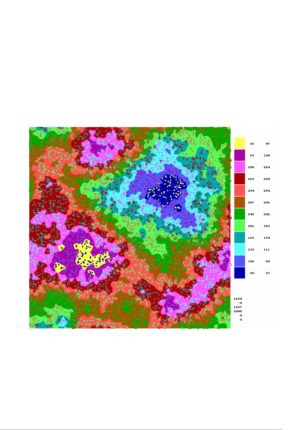
On the asymptotics of AKT statistics L ´ ıdia Rejt˝ o 1 G´ ab or T usn´ ady 2 2013. June 7:14:45 – Septem b er 15, 2013 Abstract In our da ys there is a widespread analysis of W asserstein distances b et w een theoretical and empirical measures. One of the fi rst inv estigation of the topic is giv en in the pap er written b y Ajtai, Koml´ os and T usn´ ady in 1984 . In terestingly all the neigh b oring questions p osed b y that paper w ere settled already without the original one. In this pap er we are going to delineate the limit b ehavior of the original statistics with the help of computer sim ulations. A t the same time we k ept an eye on theoretical grasping of the problem. Based on our computer sim ulations our opinion is that the limit distribution is Gaussian. 1 In tro duction Let (( X i , Y i ) , i = 1 , . . . , n ) b e indep enden t p oin ts uniformly distributed on the d dimensional unit cub e. The AKT statistic W n is the minim um of n X i =1 | X i − Y π ( i ) | 2 (1) tak en on all p ermutations π of (1 , . . . , n ) . W e call the statistics W asserstein distance. Using computer experiments we are going to in vestigate the asymptotic b eha vior of W n as d = 2 and n go es to infinity . Based on our computer sim ulations we think that if n ≤ 2048 , then the hazard rate function of the distribution of W n − β log ( n ) is prop ortional to an appropriately scaled Gaussian distribution function with β = 0 . 11 . 1 Departmen t of Applied Economics and Statistics, Universit y of Dela ware, Newark, Delaw are, USA rejto@udel.edu 2 Alfr ´ ed R ´ en yi Mathematical Institute of the Hungarian Academy of Sciences, Budap est, Hungary tusnady .gab or@ren yi.mta.h u 1 2 History The AKT statistics w ere in tro duced in [1]. In that pap er the authors pro ved that there exist p ositiv e constants c 1 , c 2 suc h that with probabilit y going to 1 c 1 log( n ) < W n < c 2 log( n ) (2) holds true. The origin of this statistic go es back to the one dimensional Shapiro–Wilks statistic for testing normality . In [2] the case d = 1 was inv estigated. The AKT statistics w ere gen- eralized in [10] while a new pro of w as given for (2) in [12]. T alagrand next inv estigated the case d ≥ 3 in [11] and settled all the observ able questions. T alagrand’s estimates for d = 2 w ere sharp ened in [7]. A broad in tro duction to transp ortation theory is presen ted in [14]. The first application of the AKT theorem w as in bin packing [5]. A n umerical inv estigation of the distribution of the statistic w as given in [8]. Matc hings on the Euclidean ball w ere inv estigated in [3]. The pap er [13] inv estigates the rate of conv ergence in abstract settings. An inv estigation of differen t types of matchings was giv en in [6]. In [4] distributions supp orted on a manifold em b edded in a Hilb ert space were in v estigated. 3 Dy adic dynamics Starting with n = 2 0 p oin ts we evolv e n = 2 k , k = 1 , 2 .. p oint pairs in such a w ay that in each step the original p oin ts remain and simultaneously a new set of point pairs are supplan ted. W e call the original kids ”old” and the new ones ”young”. Having t w o t yp es of kids, b oys and girls, there are four p ossibilities for matching: – old girls with old b oys ( O O k ), – old girls with y oung b o ys ( O Y k ), – young girls with old b o ys ( Y O k ), – young girls with young b o ys ( Y Y k ). The matc hings O O k and Y Y k are indep enden t, and similarly O Y k and Y O k are indep enden t while the costs O O k and O Y k are correlated. The cost is the W asserstein distance W n b et w een the corresp onding set of p oints. F or small v alues of n the approximation E W n = β log( n + α ) + γ is more accurate. Figure 1 shows the a verages of costs of 296 rep etitions up to k = 11 with the ab o ve theoretical function. Here α = 0 . 379 , β = 0 . 160 , γ = 0 . 117 . The densities of the normalized differences of W n − ( β log( n + α ) + γ ) are given in Figure 2. Next generation costs O O k +1 are close to the a verages ( O O k + O Y k + Y O k + Y Y k ) / 4 , 2 and the v ariance of the error is 0 . 101 . The quadratic recursion O O k +1 = ( O O k + O Y k + Y O k + Y Y k ) / 4 + V k +1 (3) with an iid noise V k +1 agrees with our conjecture indicating that the quadratic recursion might b e v alid for tw o dimensions only . In Euclidean space for arbitrary p oints a, b, c, d | ( a + b ) − ( c + d ) | 2 = | a − c | 2 + | a − d | 2 + | b − c | 2 + | b − d | 2 − | a − b | 2 − | c − d | 2 (4) holds true. Similarly in our case O O k +1 = a ∗ ( O O k + O Y k + Y O k + Y Y k ) − b ∗ ( GG k + B B k ) + V k +1 (5) holds true -where GG and B B are the girls-girls, b o ys-b o ys distances. F or stacionarity 4 ∗ a − 2 ∗ b = 1 (6) m ust b e hold. According to our computer exp eriences a = 0 . 45 , b = 0 . 41 and the error term is 0 . 06 . The distribution of the V error term seems to b e double exp onen tial. 4 Pictorial presen tation of the Hungarian Algorithm The engine of the Hungarian Algorithm is the system of shadow prices a ( i ) , b ( j ) such that b ( j ) − a ( i ) ≤ c ( i, j ) , where c ( i, j ) is the cost of the marriage of a pair ( i, j ) . In Figures 3 and 4 w e give a pictorial presen tation of the prices for n = 1024 and n = 2048 . Here w e used toroid distances and the colors of p oints of the unit square sho ws the price of the closest kid to the p oin t, i.e. the a ( i ) in case the closest kid is a girl and the b ( j ) otherwise. The k eys of colours are given on the margin. Pixel statistics are giv en for the colours, first n umber stands for wiv es, second for h usbands. E.g. in Figure 3 there are 32 yello w wives and 69 h usbands. Dark blue represen ts the minimal v alue, which is zero for the v alue of the last wife is alwa ys zero. The maximal v alue for n = 1024 is 0.02499 and it is 0.01654 for n = 2024, they are represented b y yello w colour. The kids themselv es are complementarily coloured for seeing them. Circles represen t girls, squares represent b o ys. Marriages are shown by gra y lines. F or neglecting complications of toroid top ology girls having a husband on the other side of the unit square are mark ed with an Andrew cross while their husband is not assigned. In terestingly usually there is one lak e and one hill. The actual total costs of the marriages are W 1024 = 0 . 996 , W 2048 = 1 . 654 , th us the a v erage distance in a marriage is around 0 . 02 causing the same or neighboring colours for wife and h usband. W e know that for a married couple ( i, j ) we ha ve b ( j ) − a ( i ) = c ( i, j ) , 3 hence all marriages are up w ards directed according their colour. 1024 p oint-pair from the 2048 p oin t-pairs in Figure 4 are identical with p oin t-pairs given in Figure 3, the others are generated indep enden tly . The situation not muc h changed. The b ordering lines of colours for n = 1024 are simpler than for n = 2024 . 5 Asymptotics F or the distribution of W n the b est appro ximation achiev ed b y us is a distribution determined b y its hazard rate function. Let us denote the tail distribution of a one–dimensional random v ariable b y Q ( t ) . The hazard rate r ( t ) is the deriv ativ e of − log Q ( t ) . Customarily hazard rates are defined for surviv al functions, b elonging to p ositiv e random v ariables. The concept is extendable naturally for random v ariables taking v alues b et w een −∞ and ∞ to o. Although W n is p ositive, the b est approximation comes from this broader class of distributions. The hazard rate is an arbitrary non-negative function ha ving infinite in tegral on the real line. In our case it is prop ortional to Φ( t ) the distribution function of a standard normal random v ariable. Its integral up to an x is equal to x Φ( x ) + ϕ ( x ) , where ϕ ( x ) is the standard normal densit y function. By definition it equals to − log Q ( x ). Applying the relation r ( x ) = f ( x ) /Q ( x ) , where f ( x ) stands for the density function we get f ( x ) = Φ( x ) exp( − x Φ( x ) − ϕ ( x )) . (7) The deriv ativ e of log f ( x ) is ϕ ( x ) / Φ( x ) − Φ( x ) , which is for x going to −∞ close to − x, for x going to ∞ it is going to ( − 1) and it is monotone decreasing. Th us for negativ e x -s the distribution resem bles a double exp onential distribution but for p ositive x -s it turns to b e a single exp onen tial. That is wh y f is increasing first sharply to its mo dus around 0 . 3 and it is slo wly decreasing after that v alue. W e are going to build up a three parameter family around the ab ov e distribution. The first step is Co x regression. Let λ b e arbitrary positive num ber, then ρ λ ( t ) = λ Φ( t ) is the hazard rate of the distribution with tail Q ( t ) λ and for any real µ and p ositiv e σ the linear transformation presen ts the density f ( x | µ, σ, λ ) = λ σ Φ( y ) exp( − λ ( y Φ( y ) − ϕ ( y )) , where y = ( x − µ ) /σ. (8) Let us denote b y X λ a random v ariable corresp onding to the hazard rate % λ . Let λ > 0 , σ > 0 , µ b e arbitrary real num b ers, then f ( x | µ, σ, λ ) is the density of σ X λ + µ. Th us µ is the lo cation parameter, σ is the scale parameter and λ is the shap e parameter of the distribution. Figure 5. sho ws the densit y of the distribution of X λ / ( λ ) α with α = 0 . 4, for eleven different λ from 0 . 1 to 10 . F or small λ , one can see that the distribution of X λ / ( λ ) α has an intensiv ely increasing first phase and after it b ecomes similar to the exp onen tial distribution. On the other hand for large λ it turns to b e just the opp osite. 4 The estimates of the parameters σ and λ are highly correlated, unfortunately our presen t sample size is not large enough to decide whether the v alue of the parameter λ differs signifi- can tly from 1 or not. If it do es so then the question is the tendency of λ as n go es to infinit y . With λ = 1 the tendency of σ is not clear: it is increasing from 0 . 08 up to 0 . 14 and p erhaps remains b ounded. The dynamic (5) has a second condition (not presented here) in addition to (6). It ensures the b oundedness of v ariance. F or that condition w e ha ve to know the cov ariances of the costs of different matc hings. First it w as an unsettled riddle for us what is the join t distribution for the six transp ortation costs plus error term resulting in a Gaussian hazard rate with stationary distribution. In order to settle this question the ideas of the pap er [9] turned out to b e useful: ev en the reference to the Euclidean relation (4) comes from the p ossibilit y that Euclidean relations migh t b e generalized into transp ortation equations. In the next section w e are going to discuss a partial solution of the riddle. 6 A sev en dimensional mo del F or fixed k we generate four times 2 k of p oin ts, tw o sets of girl and t wo sets of b o ys. Let us lab el then A, B , C, D . ( A is the set of old girls, B is the set of young girls, C is the set of old b o ys, and D is the set of y oung b oys.) There are six W asserstein distances among them: W 1 = ( A, C ) , W 2 = ( A, D ) , W 3 = ( B , C ) , W 4 = ( B , D ) , W 5 = ( A, B ) , W 6 = ( C , D ) . W 1 is indep enden t of W 4 and its relation with the others is symmetric. In building a joint distribution for the six v ariables w e use an autoregressiv e model: the conditional distribution of W i +1 giv en ( W 1 , . . . , W i ) , is a distribution with Gaussian hazard rate with arbitrary σ i , λ = 1 and µ i = γ i 0 + i X s =1 γ is W s . The pairs ( γ i 0 , µ i ) for k = 10 are the followings: (1 . 142 , 0 . 133) (0 . 907 , 0 . 129) (0 . 923 , 0 . 127) (0 . 706 , 0 . 125) (0 . 553 , 0 . 117) (0 . 591 , 0 . 117) . F or smaller k the tendency is similar, the leading terms γ i 0 follo w the general logarithmic trend and the σ i -s are practically the same. It go es without saying that they diverse in i . The autoregressiv e co efficients are the follo wing: 5 T able 1. γ 21 = 0 . 194 γ 31 = 0 . 176 γ 32 = 0 . 006 γ 41 = − 0 . 040 γ 42 = 0 . 188 γ 43 = 0 . 204 γ 51 = 0 . 101 γ 52 = 0 . 140 γ 53 = 0 . 126 γ 54 = 0 . 123 γ 61 = 0 . 126 γ 62 = 0 . 139 γ 63 = 0 . 138 γ 64 = 0 . 108 γ 65 = − 0 . 054 These co efficients are mostly small and they are negative for indep enden t pairs. The con- ditional distribution of ˜ W 1 for k + 1 is similar: the gammas follow the original pattern found with linear regression and the standard deviations are around 0 . 055 . W e can test the mo del in the following wa y . Having a w ell parametrized 67 dimensional distribution we can generate indep enden t 67 dimensional random v ectors as many times as man y samples we ha ve in the unit square. Presently it is 817. Next we use the Hungarian algorithm to determine the W asserstein distance of the t wo p oin t systems: it is around 1440. Finally we generate new random samples and determine their distances. Interestingly it is lar ger then 1440, its a v erage is 1470 with deviance 10. It means that the structure of the unit-square sample is a bit tighter than our autoregressiv e scheme. But a simple tric k settles the trouble: if w e multiply all standard deviation parameter σ with 0 . 975 then the unit-square W asserstein get in the middle of mo del W assersteins. If X is an arbitrary real random v ariable and Q ( x ) is its tail probabilit y P ( X > x ) , then the distribution of Q ( X ) is uniform in the interv al (0 , 1) . The integrated hazard rate R ( x ) = Z x −∞ r ( t ) dt equals to − log ( Q ( x )) , thus the distribution of R ( X ) is standard exp onential and the distri- bution of exp( − R ( X )) is again uniform in (0 , 1). So w e can test the h yp othesis that the distribution of the 67 dimensional W asserstein statistics b elongs to the three parameter family (8) testing the uniformit y of this statistics. Of course we can not use the original Kolmogorov cut-p oin ts b ecause w e use estimated parameters, w e ha ve to calibrate the cut-points b y random sample. In our case for levels 0 . 05 , 0 . 01 they are 0 . 84 , 1 . 37 . The v alue of the actual statistic is 1 . 00 since this new W assertstein statistics migh t ha v e Gaussian hazard rate. The corresponding statistics for p oin ts in the unit square are the followings. 6 T able 2. k No Kolmogorov R1 R2 R3 R4 R5 0 4902 3.0578 0.6148 0.6036 0.5354 0.6367 0.3776 1 4902 1.8130 0.7537 0.8154 0.7425 0.6165 0.5595 2 4902 1.2752 0.6765 3.6339 0.6176 0.7559 0.3969 3 4902 1.1030 0.4839 0.9168 0.5846 0.6992 5.7871 4 4902 0.9454 0.9077 0.8388 0.7162 0.5211 0.7878 5 4902 1.1828 0.5653 0.6978 0.7649 0.5019 0.5467 6 4902 1.2998 0.5306 0.5985 0.7461 0.5844 0.9778 7 4902 0.9876 0.8416 0.7448 0.5140 0.6265 0.7459 8 4902 0.9327 0.7223 0.7323 0.6713 0.9064 0.5782 9 4902 0.9697 0.8291 0.6565 0.9028 0.5890 0.7438 10 4902 1.0793 0.6249 0.6609 0.7140 0.5499 0.6290 11 817 0.6508 0.8411 0.7843 1.0557 1.1890 0.9961 Here k is num ber of num ber of doublings in the dynamics, No is the sample size. W e hav e 817 different runs and for k = 11 and the sample size for k < 11 it is 6 ∗ 817. W e multiply the maximal difference b et ween empirical and theoretical distributions with √ No but for k < 11 the W asserstein distances are not indep enden t. It might b e the reason that even for k = 10 w e hav e a b orderline result. Of course we are a ware the fact that for k = 0 the W asserstein statistics has a differen t distribution and p erhaps the situation is similar for small k -s. This tendency is clearly shown b y the Kolmogorov statistics. W e generated fiv e times data matrix b y the theoretical mo del. Columns headed b y R1,...,R5 giv es the corresp onding Kolmogorov statistics. As one can observ e the statistics ha ve rather long tail arising p erhaps from the in terw ov en dep endence structure. 7 The Ajtai statistics In pap er [1] the saddle p oin t metho d is used to prov e inequality (2). Appropriate Lipsc hitzean functions are developed to pro ve the left hand side while for the right hand side an ad-ho c matc hing algorithm due to Mikl´ os Ajtai is used. The algorithm is based on the following elemen tary concept. Definition Let s b e a p ositiv e in teger, t = 2 s and A = ( a 1 , . . . , a t ) arbitrary reals. The median bits B = ( b 1 , . . . , b t ) of A are (0 , 1)-s defined b y the prop erties t X k =1 b k = s ; if (( b i = 0) and ( b j = 1)) , then a i ≤ a j . In case there are no ties in A, B is uniquely defined. 7 Let k b e an arbitrary natural n umber, n = 4 k , and Z = ( Z i , i = 1 , . . . , n ) b e a system of arbitrary tw o-dimensional p oin ts. In a step-by-step procedure w e order a 2 k long bit sequence to eac h of the p oin ts in Z . As an initial step we construct a set A from the first co ordinates of Z . Ha ving the corresp onding B we divide Z into tw o subsets according to the bits in B and for each of that subsets we form the median bits from the second co ordinates. F rom these initializations w e pro ceed in the same manner. Using the bit sequences ordered to the points so far first w e dev elop the next bits from the subsets formed of the first coordinates ha ving the same bit sequences generated so far and next we turn to the second co ordinates. Applying the pro cedure indep enden tly for t wo iid tw o dimensional sets X and Y in the role of Z the matc hing is supplied b y the iden tical bit sequences. In course of the algorithm step by step the size of subsets is halv ed and finally it is reduced to one, thus for all p ossible 2 k long bit sequence w e ha v e exactly one p oin t in X and one in Y , and it mak es the matc hing. In a certain sense we construct a tw o-dimensional ordering merging the orders according the tw o co ordinates. Let b b e an arbitrary 2 k long bit sequence and c = k X i =1 b 2 i − 1 , d = k X i =1 b 2 i . The exp ected v alue of the first co ordinate of the corresp onding p oin ts in X or Y are lab elled by b is c/ (2 k + 1) and for the second co ordinate it is d/ (2 k + 1) . (Let us note here that in our notation X and Y are t wo sets of two dimensional p oints and the co ordinates are ( x i 1 , x i 2 ) , ( y i 1 , y i 2 )) . Let us observe that the marginal quantile transform applies for the algorithm: the match- ing itself do es not dep end on any monotone transform. (The marginal quan tile transform is F ( x i 1 ) , i = 1 , . . . , n for the first co ordinates and G ( x i 2 ) , i = 1 , . . . , n for the second co ordinates if the coordinates are indep enden t and the distribution of the first co ordinates if F and that is G for the second co ordinates.) Utilizing the mean limits offered by the algorithm we are deeply concerned that the limit distribution for an y distributions has the form n X i =1 c i x 2 i where the x i -s are indep enden t standard normals and the c i -s are appropriate co efficients. W e guess that suc h random v ariables hav e monotone increasing hazard rates, and for certain co efficien ts the hazard rate function is b ounded while for others it go es to infinity . If the m ultiplicity of the maximal co efficients is high then the leading term of the distribution has a c hi-square distribution with large degree of freedom what is approximately normal. Thus it is p ossible for the limit distributions for – W asserstein distances for uniform distribution, – W asserstein distances for standard normal distribution, – Ajtai distances for uniform distribution, – Ajtai distances for standard normal distribution, 8 all are the normal one but the sp eed of the con vergence is considerable slow. Using the marginal quan tile transformation one can ask what is the relation b et w een the distances for standard normal and uniform distributions. In the next table w e giv e the basic statistics for Ajtai distances up to 4 8 . Here D = 1 stands for standard normal and D = 2 for uniform distribution and the correlations come from marginal quan tile transformation. T able 3. k D Sample Size Av erage Stdev Sequeness Kolmogorov Lo cus Correlations 1 1 42161 9.951413 5.606661 1.261530 16.717425 23626 2 1 40184 19.597105 6.658678 0.877757 11.497639 22992 3 1 40711 34.650952 7.678610 0.663583 8.510061 21130 4 1 49367 58.719088 8.880549 0.507017 7.463537 26939 5 1 20089 97.984671 10.266948 0.334140 3.379643 8789 6 1 12988 163.848339 12.198350 0.277057 2.205296 4800 7 1 5739 276.390900 14.609538 0.130521 0.986046 2560 8 1 2333 471.869129 18.169085 0.130229 0.658314 1104 1 2 42161 0.251985 0.154344 1.114916 14.115933 21684 0.891637 2 2 40184 0.655468 0.217523 0.539991 7.161248 21916 0.858883 3 2 40711 1.428708 0.294253 0.420951 5.765374 21836 0.872925 4 2 49367 2.519040 0.360076 0.433037 6.159368 29373 0.858270 5 2 20089 3.809825 0.400688 0.401140 3.978578 12257 0.807309 6 2 12988 5.210258 0.421534 0.390273 3.757436 7405 0.734815 7 2 5739 6.669811 0.431007 0.373776 2.231697 2844 0.645670 8 2 2333 8.138648 0.438881 0.363513 1.112873 898 0.558825 Because the n umber of p oin ts 4 8 is rather large in case of the Hungarian algorithm, thus w e reduced it to 4 5 . In the next table we presen t the basic statistics for sample size 309 . T able 4. Lab el Sample type Algorithm Average St.deviation NH normal sample Hungarian algorithm 39.184 5.453 NA normal sample Ajtai algorithm 97.497 10.485 UA uniform sample Ajtai algorithm 2.902 0.541 UH uniform sample Hungarian algorithm 1.756 0.451 UB uniform sample adho c impro ving 2.224 0.500 and the correlations are the followings: 9 T able 5. NH NA UA UH UB NH 1.000 0.665 0.681 0.766 0.717 NA 0.665 1.000 0.569 0.469 0.530 UA 0.681 0.569 1.000 0.896 0.981 UH 0.766 0.469 0.896 1.000 0.942 UB 0.717 0.530 0.981 0.942 1.000 The correlation b etw een Hungarian and Ajtai algorithms for uniform distribution is 0 . 896 whic h is astonishingly high. It pro ves that the Ajtai algorithm is very efficien t. Ev en it is efficien t concerning the av erage but surprisingly it is efficient in measuring the habits of the sample for having go o d marriages. Now it is a standard observ ation for W asserstein couplings: the condition that for any finite set of marriages no reordering of the couples could improv e the sum of distances is sufficien t. F or large num ber of p oints the condition is hard to c hec k. W e use the simplest case with t wo couples, it is lab eled us “adho c improving”. One can say that it is natural that its correlation with original Ajtai is as high as 0 . 981 b ecause our ad-ho c improving starts with the Ajtai coupling. But its correlation with the optimum is also improv ed: it is now 0 . 94 . 8 Discussion The original Ajtai algorithm uses numerical medians and linear transformations fitting the medians to the interv al halving. First we apply the median of the whole set of first co ordinates and imagine a vertical line dividing the unit square accordingly . The num ber of p oints in the rectangles are equal. Next w e divide indep enden tly with appropriate horizon tal lines the left hand side and right hand side rectangles in suc h a wa y that the num ber of p oin ts in the four rectangles should b e equal. Roughly what happ en in the four rectangles are indep endent from each other if it is accordingly scaled. This concept leads to a dynamical equation similar to (3) but in this case the four terms are indep endent. This t yp e of recursion immediately leads to a normal limit distribution. When w e b eliev ed that the limit distribution is not Gaussian w e desp erately struggled against suc h kind of dynamics but no w w e are conten t that the limit distribution is Gaussian for b oth cases of Ajtai and W asserstein distance. Of course for W asserstein distance the situation is more complicated. The Ajtai algorithm works for arbitrary num ber of p oin ts, we used the p o w er of 4 only for didactical reason. 10 References [1] M. Ajtai, J. Koml´ os, and G. T usn´ ady , On optimal matchings, Combinatoric a 4/4 (1984), 259–264. [2] E. del Barrio, E. Gin ´ e, and C Matr´ an, Central limit theorems for the W asserstein distance b et w een the empirical and the true distributions, The A nnals of Pr ob ability 27/2 (1999), 1009–1071. [3] F. Barthe and N. O’Connel, Matchings and v ariance of Lipsitz functions, ESAIM: Pr ob ab. Statist. 13 (2010) 400–408. [4] G. D. Canas and L. R. Rosasco, Learning probability measures with resp ect to optimal transp ort matrices, arXiv:1209.1077v1 [cs.LG] 5 Sep 2012. [5] E. G. Coffman, Jr., M. R. Garey , and D. S. Johnson, Appr oximatio algorithms for bin p acking: an up date d survey (in A lgorithm design for c omputer systems design, G. Ausiel lo, M. Luc erfini, and P. Ser afini (e ds) pp. 49–106) , Springer, 1984. [6] A. E. Holroyd, R. Peman tle, Y. P eres, and O. Schramm, Poisson matc hings, A nn. Inst. Henri Poinc ar ´ e, Pr ob ab. Stat. 45(1) (2009) 266-289. [7] P . Ma jor, On the estimation of multiple r andom inte gr als and U–statistics (L e ctur e Notes in Mathematics) , Springer, 2013. [8] C. Nosz´ aly , Exp erimen ts on the distance of t wo–dimensional samples, Annales Mathemat- ic ae et Informatic ae 2012. [9] M.-K. v on Renesse and K.-T. Sturm, T ransp ort inequalities, gradien t estimates, entrop y and Ricci curv atures, Communic ations in Pur e and Applie d Mathematics 58/7 (2005), 923–940. [10] M. T alagrand, The Ajtai–Koml´ os–T usn´ ady matching theorem for general measures, in Pr ob ability in Banach sp ac es, 8. (Brunswick, ME, 1991) V olume 30 of Pr o gr ess in Pr ob a- bility p ages 39–54, Birkh¨ auser Boston M. 1992 [11] M. T alagrand, The transp ortation cost from the uniform measure to the empirical measure in dimension ≥ 3, The A nnls of Pr ob ability 22/2 (1994), 919–959. [12] M. T alagrand, The gener al chaining (Spinger Mono gr aphs in Mathematicics) , Springer, 2005. [13] G. L. T orrisi, Asymptotic analysis of the optimal cost in some transp ortation problems with random lo cations, Sto chastic Pr o c esses and their Applic ations 122 (2012) 305–333. [14] C. Villani, Optimal tr ansp ort: old and new , Springer, 2008 11 Figur e 1. Optimal cost as a function of the number of pairs 0 500 1000 1500 2000 0.2 0.4 0.6 0.8 1.0 1.2 n W(n) * * * * * * * * * * * * * * * * * * * * * * * * * * * * * * * * * * * * * * * * * * * * * theory estimation Figur e 2. Densities of optimal costs -0.5 0.0 0.5 1.0 0.0 0.5 1.0 1.5 2.0 2.5 3.0 3.5 x y k=0 k=1 k=2 k=3 k=4 k=5 k=6 k=7 k=8 k=9 k=10 k=11 Figur e 3. Pictorial representation of shadow prices for n=2048 Figur e 4. Pictorial representation of shadow prices for n=2048 Figur e 5. Densities for the Gaussian hazard rate model appropriately scaled