Unmixing Incoherent Structures of Big Data by Randomized or Greedy Decomposition

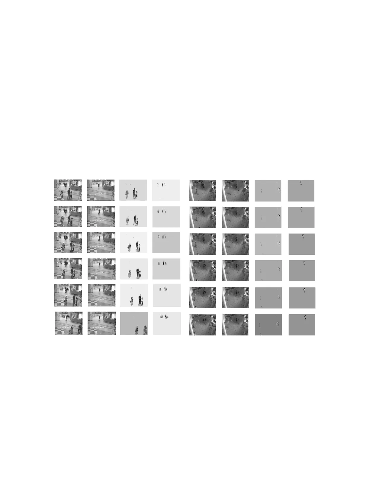
1 Unmixing Incoherent Structures of Big Data by Randomized or Greedy Decomposition T ianyi Zhou, Dacheng T ao Abstract Learning big data by matrix decomposition always suf fers from expensi ve computation, mixing of complicated structures and noise. In this paper , we study more adaptiv e models and efﬁcient algorithms that decompose a data matrix as the sum of semantic components with incoherent structures. W e ﬁrstly introduce “GO decomposition (GoDec)”, an alternating projection method estimating the low-rank part L and the sparse part S from data matrix X = L + S + G corrupted by noise G . T wo acceleration strategies are proposed to obtain scalable unmixing algorithm on big data: 1) Bilateral random projection (BRP) is de veloped to speed up the update of L in GoDec by a closed-form built from left and right random projections of X − S in lower dimensions; 2) Greedy bilateral (GreB) paradigm updates the left and right factors of L in a mutually adapti ve and greedy incremental manner , and achie ve signiﬁcant improv ement in both time and sample complexities. Then we proposes three nontri vial variants of GoDec that generalizes GoDec to more general data type and whose fast algorithms can be derived from the two strategies: 1) for motion segmentation, we further decompose the sparse S (moving objects) as the sum of multiple row-sparse matrices, each of which is a low-rank matrix after speciﬁc geometric transformation sequence and deﬁnes a motion shared by multiple objects; 2) for multi-label learning, we further decompose the low-rank L into subcomponents with separable subspaces, each corresponds to the mapping a single label in feature space. Then the prediction can be ef fectively conducted by group lasso on the subspace ensemble; 3) for estimating scoring functions of each user in recommendation system, we further decompose the low-rank L as W Z T , where the rows of W is the linear scoring functions and the ro ws of Z are the items represented by av ailable features. Empirical studies show the efﬁcienc y , robustness and ef fectiveness of the proposed methods in real applications. Index T erms Low-rank and sparse matrix decomposition, bilateral random projection, greedy bilateral paradigm, multi-label learning, background modeling, motion segmentation, recommendation systems I . I N T RO D U C T I O N Complex data is usually generated by mixing se veral components of dif ferent structures. These structures are often compressible, and are able to provide semantic interpretations of the data May 2, 2022 DRAFT 2 content. In addition, they can rev eal the difference and similarity among data samples, and thus produce robust features playing vital roles in supervised or unsupervised learning tasks. T wo types of structures hav e drawn lots of research attentions in recent years: 1) in compressed sensing [1], [2], a sparse signal can be exactly recovered from its linear measurements at a rate signiﬁcant belo w the Nyquist rate, in sparse coding [3], [4], [5], an ov er-complete dictionary leads to sparse representations for dense signals of the same type; 2) in matrix completion [6], [7], [8], [9], [10], a low-rank matrix can be precisely rebuilt from a small portion of its entries by restricting the rows (samples) to lie in a subspace. In dimension reduction [11], [12], [13], [14], [15], [16], lo w-rank structure [17] has been broadly le veraged for exploring the geometry of point cloud. Although sparse and low-rank structures ha ve been studied separately by a great number of researchers for years, the linear combination of them or their e xtensions is rarely explored until recently [18], [19], [20], [21]. Intuitiv ely , ﬁtting data with either sparse or lo w- rank structure is mature technique but is inevitably restricted by the limited data types they can model, while recent study sho ws that the linear mixture of them is more expressi ve in modeling complex data from different applications. A motiv ating e xample is robust PCA [19] (RPCA), which decomposes the data matrix X as L + S . The low-rank part L summarizes a subspace that is shared by all the samples and thus rev eals the global smoothness, while the sparse part S captures the indi vidual dif ferences or abrupt changes among samples. A direct application of rob ust PCA is separating the sparse moving objects from the low-rank background in video sequence. Another interesting example is morphological component analysis (MCA) [22], which decompose the data into tw o parts that hav e sparse representations on two incoherent ov er-complete dictionaries, i.e., the ﬁrst part has a very non-sparse representation on the dictionary of the second part, and vise versa. This requirement suggests that the two parts are separable on their sparse representations. Note that both RPCA and MCA can only work on data whose two building parts are incoherent, i.e., the content of one part cannot be mov ed to the other part without changing either of their structures (low-rank, sparse, dictionary , etc.). This incoherence condition could be viewed as a general extension of the statistical independence supporting independent component analysis (ICA) [23], [24] blindly separating non-Gaussian source signals. It leads to the identiﬁability of the structures in theory , and is demonstrated to be fulﬁlled on a wide class of real data. Ho wev er , ne w challenges arises when many recent studies tend to focus on big data with complex structures. Firstly , existing algorithms are computationally prohibitiv e to processing these data. For instance, the update of low-rank part in RPCA and in its extensions in voke a full singular v alue decomposition (SVD) per iterate, while MCA requires challenging ` 0 or ` 1 minimization per sample/feature and pre viously achiev ed incoherent dictionaries/transform May 2, 2022 DRAFT 3 operators encouraging sparse representations. Thus they suf fer from a dramatic gro wth in time complexity when either feature dimensions or data samples increase. In pre vious methods, the structured information such as low-rank and sparse properties are always achieved at the price of time-consuming optimization, but are rarely le veraged for the purpose of improving the scalability . Recent progresses in randomized approximation and rank-rev ealing algorithms shed some light on the speedup of the robust PCA typed algorithms: the subspace of the low-rank part can be estimated from random sampling of its columns/rows or projections of its columns/ro ws on a random ensemble with bounded precision [25], [26], [27]. Ho wev er , straightforward in voking this technique in RPCA problem needs to apply it to the updated residual matrix per iterate and thus may lead to costly computation. Besides, determining the rank of the low-rank part is not a trivial problem in practice. Secondly , the simple low-rank, sparse and sparse representation assumptions cannot fully capture the sophisticated relation, indi viduality and sparsity of data samples with complex structures. While low-rank structure summarizes a global linear relationship between data points, the nonlinear relationship, local geometry and correlated functions are more common in big data and more expressi ve for a much wider class of structures. Moreover , the sparse matrix is simply explained by random noises on random positions in the past, but current studies rev eal that it may hav e rich structured information that could be the central interests of v arious applications. For instance, the sparse motions captured by RPCA on video sequence data includes immense unexplored information fa vored by object tracking and beha vior analysis. Furthermore, although the sparse representation is more general than sparse features, its quality largely relies on whether the gi ven dictionary or transform operator ﬁts the nature of data well. But this is difﬁcult to e valuate when the data is of large volume and in general type. Thirdly , two building parts are not suf ﬁcient to cover all the mixtures of incoherent structures in big data. One the one hand, dense noise is an extra component that has to be separated from the lo w-rank and sparse parts in many cases where the exact decomposition X = L + S does not hold. This noisy assumption has been considered in stable PCP [28], DRMF [29] and other theoretical studies [20], and its rob ustness and adaptiv eness to a broad class of data has also been veriﬁed. But efﬁcient algorithm for the noisy model lacks. On the other hand, further decomposing the lo w-rank or sparse part to multiple distinguishable sub-components is potential to tell locally spatial or temporal relations within each identiﬁable structure and dif ferences between them, which usually play pi vot roles in supervised and unsupervised learning tasks. Although it appeals to be a natural extension to the two-part model in RPCA, ho w to formulate a proper decomposition model for learning problems and dev elop a practical algorithm are challenging. May 2, 2022 DRAFT 4 A. Main Contrib utions W e start this paper by studying a no vel lo w-rank and sparse matrix decomposition model “GO decomposition (GoDec)” [30] X = L + S + G , which takes an extra dense noisy part G into account and casts the decomposition into alternating optimization of lo w-rank L and sparse S . In order to ov ercome the computational burden caused by the large volume of data, we propose two acceleration strategies in designing the decomposition algorithms: the ﬁrst is “bilateral random projection (BRP)” [31] based fast lo w-rank approximation that results in a randomized update of the lo w-rank part or its nonlinear variant, this technique is based on recently de veloped random matrix theories that sho w a few random projections of a matrix is able to re veal its associated principle subspace [32], [25], [26], [27]; the other is a Frank-W olfe typed optimization scheme called “greedy bilateral (GreB)” paradigm [33] that updates the left and right factors of the lo w-rank matrix v ariable in a mutually adaptiv e and greedy incremental manner . W e show the two strategies generates considerably scalable algorithms for low-rank and sparse matrix decomposition. Moreover , both strategies hav e pro vable performance guarantee gi ven by rigorous theoretical analysis (Appendix I and II). In order to deal with the complicated structures that cannot be captured by the sum mixture of lo w-rank and sparse matrices, we proposes three variants of GoDec more expressi ve and general for learning from big data. The ﬁrst variant “shifted subspace tracking (SST)” [34] is de veloped for motion segmentation [35], [36], [37], [38], [39] from raw pix els of video sequence. SST further analyzes the unexplored rich structure of the sparse part S of GoDec, which could be seem as a sum mixture of se veral motions with distinct appearance and trajectories. SST uniﬁes detection, tracking and segmenting multiple motions from complex scenes in a simple matrix factorization model. The second v ariant “multi-label subspace ensemble (MSE)” [40] extends the low-rank part L of GoDec to the sum of multiple low-rank matrices deﬁned by distinguishable but correlated subspaces. MSE provides a novel insight into the multi-label learning (ML) problem [41], [42], [43], [44], [45]. It addresses this problem by jointly learning inv erse mappings that map each label to the feature space as a subspace, and formulating the prediction as ﬁnding the group sparse representation [46] of a gi ven sample on the ensemble of subspaces. There are only k subspaces needed to be learned, and the label correlations are fully used via considering correlation among subspaces. The third v ariant “linear functional GoDec (LinGoDec)” learns scoring functions of users from their ratings matrix X and features of scored items Z . It extends the low-rank part L of GoDec to W Z T , where W represents the linear functions and is constrained to be lo w-rank, while the rows of Z contain the features of items in the training set. In addition, the sparse May 2, 2022 DRAFT 5 part S is able to detect the advertising ef fects or anomaly of users’ ratings on speciﬁc items. LinGoDec formulates the collaborati ve ﬁltering problem as supervised learning, and thus av oids time-consuming completion of the whole matrix when only a new item’ s scores (a new row) are needed to be predicted. The rest of this paper is organized as follo wing: Section 2 introduces GoDec; Section 3 proposes the two acceleration strategies for processing large-scale data; Section 4 proposes the three variants of GoDec and their practical algorithms; Section 5 sho ws the experimental results of all the proposed algorithms on dif ferent application problems and justiﬁes both the ef fectiv eness and ef ﬁciency of them. The rows of all data matrices mentioned in this paper represents the samples and the columns denote the features. I I . G O D E C O M P O S I T I O N : U N M I X I N G L O W - R A N K A N D S PA R S E S T R U C T U R E S In RPCA [19], PCP reco vers L and S from X by minimizing sum of the trace norm of L and the ` 1 norm of S . It can be prov ed that the solution to this con ve x relaxation is the exact recov ery if X = L + S indeed exists and L and S are sufﬁciently incoherent [18], [19]. That is, L obeys the incoherence property and thus is not sparse, while S has nonzero entries uniformly selected at random and thus is not low-rank. Popular optimization algorithms such as augmented Lagrangian multiplier , accelerated proximal gradient method and accelerated projected gradient method [21] have been applied. But full SVD as a costly subroutine is required to be repeatedly in vok ed in any of them. Despite the strong theoretical guarantee of robust PCA, the exact decomposition X = L + S does not always hold for real data matrix X due to extra noise and complicated structure of S that does not following Bernoulli-Gaussian distrib ution. Thus a more adapti ve model X = L + S + G is preferred, where L + S approximates X and G is the dense noise. W e then study the approximated “lo w-rank+sparse” decomposition of a matrix X , i.e., X = L + S + G, rank( L ) ≤ r, card( S ) ≤ k , (1) In this section, we develop “Go Decomposition” (GoDec) to estimate the low-rank part L and the sparse part S from X by solving the follo wing optimization problem, which aims at minimizing the decomposition error: min L,S k X − L − S k 2 F s.t. rank ( L ) ≤ r , card ( S ) ≤ k . (2) May 2, 2022 DRAFT 6 A. Na ¨ ıve GoDec W e propose the na ¨ ıve GoDec algorithm at ﬁrst and will study how to achieve an highly accelerated version in the next section. The optimization problem of GoDec (2) can be solved by alternativ ely solving the following two subproblems until conv ergence:      L t = arg min rank( L ) ≤ r k X − L − S t − 1 k 2 F ; S t = arg min card( S ) ≤ k k X − L t − S k 2 F . (3) Although both subproblems (3) ha ve noncon vex constraints, their global solutions L t and S t exist. Let the SVD of a matrix X be U Λ V T and λ i or λ i ( X ) stands for the i th largest singular v alue of X ; P Ω ( · ) is the projection of a matrix to an entry set Ω . In particular , the two subproblems in (3) can be solved by updating L t via singular value hard thresholding of X − S t − 1 and updating S t via entry-wise hard thresholding of X − L t , respecti vely , i.e.,            L t = r P i =1 λ i U i V T i , svd ( X − S t − 1 ) = U Λ V T ; S t = P Ω ( X − L t ) , Ω :    ( X − L t ) i,j ∈ Ω    6 = 0 and ≥    ( X − L t ) i,j ∈ Ω    , | Ω | ≤ k . (4) The main computation in the na ¨ ıve GoDec algorithm (4) is the SVD of X − S t − 1 in the updating L t sequence. SVD requires min ( mn 2 , m 2 n ) ﬂops, so it is impractical when X is of large size, and more efﬁcient algorithm is needed to be dev eloped later . GoDec alternati vely assigns the r -rank approximation of X − S to L and assigns the sparse approximation with cardinality k of X − L to S . The updating of L is obtained via singular value hard thresholding of X − S , while the updating of S is obtained via entry-wise hard thresholding [47] of X − L . The term “GO” is owing to the similarities between L / S in the GoDec iteration rounds and the two players in the game of go. Except the additional noisy part G and faster speed, the direct constraints to the rank of L and the cardinality S also makes GoDec different from RPCA minimizing their con vex polytopes. This makes the rank and cardinality controllable, which is preferred in practice. Because prior information of these two parameters can be applied and lots of computations might be saved. In addition, GoDec introduces an ef ﬁcient matrix completion algorithm [30], in which the cardinality constraint is replaced by a ﬁxed support set. Con ver gence and robustness analysis of GoDec is gi ven in Appendix I based on theory of alternating projection on two manifolds [48]. May 2, 2022 DRAFT 7 I I I . T W O A C C E L E R A T I O N S T R A T E G I E S F O R U N M I X I N G I N C O H E R E N T S T R U C T U R E S W e ﬁrstly introduce the bilateral random projections (BRP) based lo w-rank approximation and its po wer scheme modiﬁcation. BRP reduces the time consuming SVD in na ¨ ıve GoDec to a closed-form approximation merely requiring small matrix multiplications. Ho wev er, we need to in vok e more expensi ve power scheme of BRP when the matrix spectrum does not have dramatic decreasing. Moreov er , the rank needs to be estimated for saving unnecessary computations. Thus we propose greedy bilateral sketch (GreBske), which augments the matrix factors column/rows- wisely by selecting the best rank-one directions for approximation. It can adaptiv ely determines the rank by stopping the augmenting when error is suf ﬁciently small, and has accuracy closer to SVD. A. Bilateral Random Pr ojection based Strate gy 1) Low-rank appr oximation with closed form: Giv en r bilateral random projections (BRP) of an m × n dense matrix X (w .l.o.g, m ≥ n ), i.e., Y 1 = X A 1 and Y 2 = X T A 2 , wherein A 1 ∈ R n × r and A 2 ∈ R m × r are random matrices, L = Y 1  A T 2 Y 1  − 1 Y T 2 (5) is a fast rank- r approximation of X . The computation of L includes an in verse of an r × r matrix and three matrix multiplications. Thus, for a dense X , 2 mnr ﬂoating-point operations (ﬂops) are required to obtain BRP , r 2 (2 n + r ) + mnr ﬂops are required to obtain L . The computational cost is much less than SVD based approximation. In order to improv e the approximation precision of L in (5) when A 1 and A 2 are standard Gaussian matrices, we use the obtained right random projection Y 1 to build a better left projection matrix A 2 , and use Y 2 to build a better A 1 . In particular , after Y 1 = X A 1 , we update A 2 = Y 1 and calculate the left random projection Y 2 = X T A 2 , then we update A 1 = Y 2 and calculate the right random projection Y 1 = X A 1 . A better low-rank approximation L will be obtained if the ne w Y 1 and Y 2 are applied to (5). This improvemen t requires additional ﬂops of mnr in BRP calculation. 2) P ower scheme modiﬁcation: When singular values of X decay slo wly , (5) may perform poorly . W e design a modiﬁcation for this situation based on the po wer scheme [49]. In the po wer scheme modiﬁcation, we instead calculate the BRP of a matrix ˜ X = ( X X T ) q X , whose singular v alues decay faster than X . In particular , λ i ( ˜ X ) = λ i ( ˜ X ) 2 q +1 . Both X and ˜ X share the same singular vectors. The BRP of ˜ X is: Y 1 = ˜ X A 1 , Y 2 = ˜ X T A 2 . (6) May 2, 2022 DRAFT 8 According to (5), the BRP based r rank approximation of ˜ X is: ˜ L = Y 1  A T 2 Y 1  − 1 Y T 2 . (7) In order to obtain the approximation of X with rank r , we calculate the QR decomposition of Y 1 and Y 2 , i.e., Y 1 = Q 1 R 1 , Y 2 = Q 2 R 2 . (8) The low-rank approximation of X is then giv en by: L =  ˜ L  1 2 q +1 = Q 1 h R 1  A T 2 Y 1  − 1 R T 2 i 1 2 q +1 Q T 2 . (9) The power scheme modiﬁcation (9) requires an in verse of an r × r matrix, an SVD of an r × r matrix and ﬁ ve matrix multiplications. Therefore, for dense X , 2(2 q + 1) mnr ﬂops are required to obtain BRP , r 2 ( m + n ) ﬂops are required to obtain the QR decompositions, 2 r 2 ( n + 2 r ) + mnr ﬂops are required to obtain L . The po wer scheme modiﬁcation reduces the error of (5) by increasing q . When the random matrices A 1 and A 2 are built from Y 1 and Y 2 , mnr additional ﬂops are required in the BRP calculation. Thorough error bound analysis of BRP and its power scheme is given in Appendix II. 3) F ast GoDec by Bilateral Random Pr ojection: Since BRP based low-rank approximation is near optimal and ef ﬁcient, we replace SVD with BRP in na ¨ ıve GoDec in order to signiﬁcantly reduce the time cost. W e summarize GoDec using BRP based low-rank approximation (5) and power scheme modi- ﬁcation (9) in Algorithm 1. When q = 0 , For dense X , (5) is applied. Thus the QR decomposition of Y 1 and Y 2 in Algorithm 1 are not performed, and L t is updated as L t = Y 1  A T 2 Y 1  − 1 Y T 2 . In this case, Algorithm 1 requires r 2 (2 n + r ) + 4 mnr ﬂops per iteration. When integer q > 0 , (9) is applied and Algorithm 1 requires r 2 ( m + 3 n + 4 r ) + (4 q + 4) mnr ﬂops per iteration. B. Gr eedy Bilateral F actorization Strate gy The major computation in na ¨ ıve GoDec is the update of the low-rank part L , which requires at least a truncated SVD. Although the proposed randomized strategy provides a faster and SVD-free algorithm for GoDec, ho w to determine the rank of L and the cardinality of S is still an unsolv ed problem in real applications. In fact, these tw o parameters are not easy to determine and could lead to unstable solutions when estimated incorrectly . Noisy rob ust PCA methods such as stable PCP [28], GoDec [30] and DRMF [29] usually suffer from this problem. Another shortcoming of the randomized strategy is that the time comple xity is dominated by matrix multiplications, which could be computationally slow on high-dimensional data. May 2, 2022 DRAFT 9 Algorithm 1: GO Decomposition (GoDec) by BRP Input : X , r , k ,  , q Output : L , S Initialize L 0 := X , S 0 := 0 , t := 0 ; while k X − L t − S t k 2 F / k X k 2 F >  do t := t + 1 ; ˜ L = h ( X − S t − 1 ) ( X − S t − 1 ) T i q ( X − S t − 1 ) ; Y 1 = ˜ LA 1 , A 2 = Y 1 ; Y 2 = ˜ L T Y 1 = Q 2 R 2 , Y 1 = ˜ LY 2 = Q 1 R 1 ; If rank  A T 2 Y 1  < r then r := rank  A T 2 Y 1  , go to the ﬁrst step; end ; L t = Q 1 h R 1  A T 2 Y 1  − 1 R T 2 i 1 / (2 q +1) Q T 2 ; S t = P Ω ( X − L t ) , Ω is the nonzero subset of the ﬁrst k largest entries of | X − L t | ; end In this part, we describe and analyze a general scheme called “greedy bilateral (GreB)” paradigm for solving optimizing low-rank matrix in mainstream problems. In GreB, the lo w-rank v ariable L is modeled in a bilateral factorization form U V , where U is a tall matrix and V is a fat matrix. It starts from U and V respecti vely containing a very few (e.g., one) columns and ro ws, and optimizes them alternately . Their updates are based on observ ation that the object v alue is determined by the product U V rather than individual U or V . Thus we can choose a dif ferent pair ( U, V ) producing the same U V b ut computed faster than the one deriv ed by alternating least squares like in IRLS-M [50] and ALS [51]. In GreB, the updates of U and V can be vie wed as mutually adapti ve update of the left and right sketches of the lo w-rank matrix. Such updates are repeated until the object conv ergence, then a fe w more columns (or ro ws) are concatenated to the obtained U (or V ), and the alternating updates are restarted on a higher rank. Here, the added columns (or ro ws) are selected in a greedy manner . Speciﬁcally , they are composed of the rank- 1 column (or row) directions on which the object decreases fastest. GreB incrementally increases the rank until when U V is adequately consistent with the observations. GreB’ s greedy strategy av oids the failures brought by possible biased rank estimation. More- ov er , greedy selecting optimization directions from 1 to r is faster than updating r directions in all iterates like in LMaFit [52] and [30]. In addition, the lo wer rank solution before each rank increment is in voked as the “warm start” of the next higher rank optimization and thus speed up con ver gence. Furthermore, its mutually adapti ve updates of U and V yields a simple yet efﬁcient SVD-free implementation. Under GreB paradigm, the overall time comple xity of matrix completion is O (max {k Ω k 0 r 2 , ( m + n ) r 3 } ) ( Ω -sampling set, m × n -matrix size, r -rank), while the ov erall complexities of lo w-rank approximation and noisy robust PCA are O ( mnr 2 ) . May 2, 2022 DRAFT 10 Algorithm 2: Greedy Bilateral (GreB) Paradigm Input : Object function f ; rank step size ∆ r ; power K ; tolerance τ ; observations of data matrix X Output : low-rank matrix U V and sparse S Initialize V ∈ R r 0 × n (and S ); while residual err or ≤ τ do for k ← 1 to K do Update U , V and S by alternating minimization rules, other faster U and V update rules can be applied if they produce equal U V ; Greedy Bilateral Smoothing: sequentially compute (13); end Calculate the top ∆ r right singular vectors v (or ∆ r -dimensional random projections) of ∂ f /∂ V (for GreBsmo compute (14)); Set V := [ V ; v ] ; end An improvement on sample complexity can also be justiﬁed. An theoretical analysis of GreB solution con ver gence based on the result of GECO [53] is giv en in Appendix III. In the following, we present GreB by using it to deriv e a practical algorithm “greedy bilateral smoothing (GreBsmo)” for GoDec. It can also be directly applied to low-rank approximation and matrix completion []. W e summarize general GreB paradigm in Algorithm 2, and then present the detailed GreBsmo algorithm. 1) F aster GoDec by Gr eedy Bilateral Smoothing: In particular , we formulate GoDec by replacing L with its bilateral factorization L = U V and regularizing the ` 1 norm of S ’ s entries: min U,V ,S k X − U V − S k 2 F + λ k v ec( S ) k 1 s . t . r ank ( U ) = r ank ( V ) ≤ r. (10) Note the ` 1 regularization is a minor modiﬁcation to the cardinality constraint in (2). It induces soft-thresholding in updating S , which is faster than sorting caused by cardinality constraint in GoDec and DRMF . Alternately optimizing U , V and S in (10) immediately yields the following updating rules:      U k = ( X − S k − 1 ) V T k − 1  V k − 1 V T k − 1  † , V k =  U T k U k  † U T k ( X − S k − 1 ) , S k = S λ ( X − U k V k ) , (11) where S λ is an element-wise soft thresholding operator with threshold λ such that S λ X = { sgn ( X ij ) max ( | X ij | − λ, 0) : ( i, j ) ∈ [ m ] × [ n ] } . (12) May 2, 2022 DRAFT 11 The same trick of replacing the ( U, V ) pair with a faster computed one is applied and produce      U k = Q, QR  ( X − S k − 1 ) V T k − 1  = QR, V k = Q T ( X − S k − 1 ) , S k = S λ ( X − U k V k ) , (13) The above procedure can be performed in 3 mnr i + mr 2 i ﬂops for U ∈ R m × r i and V ∈ R r i × n . In GreBsmo, (13) is iterated as a subroutine of GreB’ s greedy incremental paradigm. In particular , the updates in (13) are iterated for K times or until the object con ver ging, then ∆ r ro ws are added into V as the new directions for decreasing the object value. In order to achiev e the fastest decreasing directions, we greedily select the added ∆ r rows as the top ∆ r right singular vectors of the partial deriv ati ve ∂ k X − U V − S k 2 F ∂ V = X − U V − S. (14) W e also allo w to approximate ro w space of the singular vectors via random projections [25]. The selected ∆ r ro ws maximize the magnitude of the above partial deriv ati ve and thus lead to the most rapid decreasing of the object value, a.k.a., the decomposition error . GreBsmo repeatedly increases the rank until a sufﬁciently small decomposition error is achiev ed. So the rank of the lo w-rank component is adaptively estimated in GreBsmo and does not relies on initial estimation. I V . T H R E E V A R I A N T S O F G O D E C Although the two strategies successfully generate efﬁcient low-rank and sparse decomposition capable to tackle large volume problem of big data, the complicated structures widely existing in big data cannot be always expressed by the sum of low-rank and sparse matrices and thus may still lead to the failure of RPCA typed models. Therefore, we address this problem by de veloping sev eral GoDec’ s variants that unrav el different combination of incoherent structures beyond lo w-rank and sparse matrices, where the two strategies can be still used to achiev e scalable algorithms. A. Shifted Subspace T racking (SST) for Motion Se gmentation SST decomposes S of GoDec into the sum of sev eral matrices, each of whose rows are generated by imposing a smooth geometric transformation sequence to the ro ws of a low- rank matrix. These ro ws store moving object in the same motion after aligning them across dif ferent frames, while the geometric transformation sequence deﬁnes the shared trajectories and deformations of those moving objects across frames. In the following, we dev elop an efﬁcient randomized algorithm extracting the motions in sequel, where the low-rank matrix for each May 2, 2022 DRAFT 12 motion is updated by BRP , and the geometric transformation sequence is updated in a piece- wise linear approximation manner . W e consider the problem of motion segmentation from the raw video data. Giv en a data matrix X ∈ R n × p that stores a video sequence of n frames, each of which has w × h = p pixels and reshaped as a row vector in X , the goal of SST framew ork is to separate the motions of dif ferent object ﬂows, recov er both their low-rank patterns and geometric transformation sequences. This task is decomposed as two steps, background modeling that separates all the mo ving objects from the static background, and ﬂo w tracking that recov ers the information of each motion. In this problem, · i stands for the i th entry of a vector or the i th ro w of a matrix, while · i,j signiﬁes the entry at the i th ro w and the j th column of a matrix. The ﬁrst step can be accomplished by either GoDec or GreBsmo. After obtaining the sparse outliers S storing multiple motions, SST treats the sparse matrix S as the ne w data matrix X , and decomposes it as X = P k i =1 ˜ L ( i ) + S + G , wherein ˜ L ( i ) denotes the i th motion, S stands for the sparse outliers and G stands for the Gaussian noise. The motion segmentation in SST is based on an observation to the implicit structures of the sparse matrix ˜ L ( i ) . If the trajectory of the object ﬂow ˜ L ( i ) is known and each frame (ro w) in ˜ L ( i ) is shifted to the position of a reference frame, due to the limited number of poses for the same object ﬂo w in different frames, it is reasonable to assume that the rows of the shifted ˜ L ( i ) exist in a subspace. In other words, ˜ L ( i ) after in verse geometric transformation is lo w-rank. Hence the sparse motion matrix ˜ L ( i ) has the following structured representation ˜ L ( i ) =     L ( i ) 1 ◦ τ ( i ) 1 . . . L ( i ) n ◦ τ ( i ) n     = L ( i ) ◦ τ ( i ) . (15) The in vertible transformation τ ( i ) j : R 2 → R 2 denotes the 2-D geometric transformation (to the reference frame) associated with the i th motion in the j th frame, which is represented by L ( i ) j . T o be speciﬁc, the j th ro w in ˜ L ( i ) is L ( i ) j after certain permutation of its entries. The permutation results from applying the nonlinear transformation τ ( i ) j to each nonzero pix el in L ( i ) j such that, τ ( i ) j ( x, y ) = ( u, v ) , (16) where τ ( i ) j could be one of the ﬁv e geometric transformations [54], i.e., translation, Euclidean, similarity , afﬁne and homography , which are able to be represented by 2 , 3 , 4 , 6 and 9 free parameters, respectiv ely . For example, afﬁne transformation is deﬁned as " u v # = " ρ cos θ ρ sin θ − ρ sin θ ρ cos θ # " x y # + " t x t y # , (17) May 2, 2022 DRAFT 13 wherein θ is the rotation angle, t x and t y are the two translations and ρ is the scaling ratio. It is worth to point out that τ ( i ) j can be any other transformation beyond the geometric group. So SST can be applied to sparse structure in other applications if parametric form of τ ( i ) j is kno wn. W e deﬁne the nonlinear operator ◦ as ˜ L ( i ) j,u +( v − 1) h = ( L ( i ) j ◦ τ ( i ) j ) u +( v − 1) h = L ( i ) j,x +( y − 1) h . (18) Therefore, the ﬂow tracking in SST aims at decomposing the sparse matrix X ( S obtained in the background modeling) as X = k P i =1 L ( i ) ◦ τ ( i ) + S + G, rank ( L ( i )) ≤ r i , card( S ) ≤ s. (19) In SST , we iterati vely inv oke k times of the following matrix decomposition to greedily construct the decomposition in (19): X = L ◦ τ + S + G, rank ( L ) ≤ r, card( S ) ≤ s. (20) In each time of the matrix decomposition abov e, the data matrix X is S obtained by former decomposition. In order to sav e the computation and facilitate the parameter tuning, we cast the decomposition (20) into an optimization similar to (2), min L,τ ,S k X − L ◦ τ − S k 2 F + λ k S k 1 s.t. rank ( L ) ≤ r , (21) Flo w tracking in SST solves a sequence of optimization problem of type (21). Thus we ﬁrstly apply alternating minimization to (21). This results in iterati ve update of the solutions to the follo wing three subproblems,          τ t = arg min τ k X − L t − 1 ◦ τ − S t − 1 k 2 F ; L t = arg min rank( L ) ≤ r k X − L ◦ τ t − S t − 1 k 2 F ; S t = arg min S k X − L t ◦ τ t − S k 2 F + λ k S k 1 . (22) 1) Update of τ : The ﬁrst subproblem aims at solving the following series of nonlinear equations of τ j , L t − 1 j ◦ τ j = X j − S t − 1 j , j = 1 , · · · , n. (23) Albeit directly solving the abov e equation is difﬁcult due to its strong nonlinearity , we can approximate the geometric transformation L t − 1 j ◦ τ j by using piece-wise linear transformations, where each piece corresponds to a small change of τ j deﬁned by ∆ τ j . Thus the solution of (23) May 2, 2022 DRAFT 14 can be approximated by accumulating a series of ∆ τ j . This can be vie wed as an inner loop included in the update of τ . Thus we have linear approximation L t − 1 j ◦ ( τ j + ∆ τ j ) ≈ L t − 1 j ◦ τ j + ∆ τ j J j , (24) where J j is the Jacobian of L t − 1 j ◦ τ j with respect to the transformation parameters in τ j . Therefore, by substituting (24) into (23), ∆ τ j in each linear piece can be solved as ∆ τ j =  X j − S t − 1 j − L t − 1 j ◦ τ j  ( J j ) † . (25) The update of τ j starts from some initial τ j , and iterativ ely solv es the o verdetermined linear equation (25) with update τ j := τ j + ∆ τ j until the difference between the left hand side and the right hand side of (23) is sufﬁciently small. It is critical to emphasize that a well selected initial v alue of τ j can signiﬁcantly save computational time. Based on the between-frame afﬁnity , we initialize τ j by the transformation of its adjacent frame that is closer to the template frame s , τ j := ( τ j +1 , j < s ; τ j − 1 , j > s . (26) Another important support set constraint, supp( L ◦ τ ) ⊆ supp( X ) , needs to be considered in calculating L t − 1 j ◦ τ j during the update of τ . This constraint ensures that the object ﬂows or segmented motions obtained by SST always belong to the sparse part achie ved from the back- ground modeling, and thus rules out the noise in background. Hence, suppose the complement set of supp( X j ) to be supp c ( X j ) , each calculation of L t − 1 j ◦ τ j follo ws a screening such that,  L t − 1 j ◦ τ j  supp c ( X j ) = − → 0 . (27) 2) Update of L : The second subproblem has the follo wing global solution that can be updated by BRP based low-rank approximation (5) and its power scheme modiﬁcation, L t = r X i =1 λ i U i V T i , svd  X − S t − 1  ◦ τ − 1  = U Λ V T , (28) wherein τ − 1 denotes the in verse transformation to wards τ . The SVDs can be accelerated by BRP based lo w-rank approximation (2). Another acceleration trick is based on the fact that most columns of ( X − S t − 1 ) ◦ τ − 1 are nearly all-zeros. This is because the object ﬂow or motion after transformation occupies a very small area of the whole frame. Therefore, The update of L t can be reduced to low-rank approximation of a submatrix of ( X − S t − 1 ) ◦ τ − 1 that only includes dense columns. Since the number of dense columns is f ar less than p , the update of L t can become much faster . May 2, 2022 DRAFT 15 3) Update of S : The third subproblem has a global solution that can be obtained via soft- thresholding P λ ( · ) similar to the update of S in GreBsmo, S t = P λ  X − L t ◦ τ t  . (29) Algorithm 3: Shifted Subspace Tracking (SST) Input : X , r i , λ i ( i = 1 , · · · , n ) , k Output : L i ( i = 1 , · · · , n ) , S for i ← 1 to k do Initialize: s = arg max i card ( X i ) ; L = [ X s ; · · · ; X s ] , S = 0 , τ = − → 0 ; while not conver ge do for j ← s − 1 to 1 do τ j := τ j +1 ; while not conver ge do ˜ L t − 1 j = L t − 1 j ◦ τ j , ˜ L t − 1 j, supp c ( X j ) = − → 0 ; τ j := τ j +  X j − S t − 1 j − ˜ L t − 1 j  ( J j ) † ; end end for j ← s + 1 to n do τ j := τ j − 1 ; while not conver ge do ˜ L t − 1 j = L t − 1 j ◦ τ j , ˜ L t − 1 j, supp c ( X j ) = − → 0 ; τ j := τ j +  X j − S t − 1 j − ˜ L t − 1 j  ( J j ) † ; end end τ t = τ ; L t = BRP  X − S t − 1  ◦ τ − 1  ; S t = P λ  X − L t ◦ τ t  , S t j, supp c ( X j ) = − → 0 ; end X := S t , L ( i ) := L t , τ ( i ) = τ t ; end A support set constraint supp( S ) ⊆ supp( X ) should be considered in the update of S as well. Hence the above update follows a postprocessing, S t j, supp c ( X j ) = − → 0 , j = 1 , · · · , n. (30) Note the transformation computation ◦ in the update can be accelerated by le veraging the sparsity of the motions. Speciﬁcally , the sparsity allows SST to only compute the transformed positions of the nonzero pixels. W e summarize the SST algorithm in Algorithm 3. B. Multi-label Subspace Ensemble MSE provides a no vel insight into the multi-label learning (ML) problem, which aims at predicting multiple labels of a data sample. Most previous ML methods [55], [56], [57], [58], May 2, 2022 DRAFT 16 [59], [60] focus on training effecti ve classiﬁers that establishes a mapping from feature space to label space, and take the label correlation into account in the training process. Because it has been longly believed that label correlation is useful for improving prediction performance. Ho wev er , in these methods, both the label space and the model complexity will grow rapidly when increasing the number of labels and simultaneously modeling their joint correlations. This usually makes the av ailable training samples insufﬁcient for learning a joint prediction model. MSE eliminates this problem by jointly learning in verse mappings that map each label to the feature space as a subspace, and formulating the prediction as ﬁnding the group sparse representation [46] of a gi ven sample on the ensemble of subspaces. In the training stage, the training data matrix X is decomposed as the sum of sev eral lo w-rank matrices and a sparse residual via a randomized optimization. Each low-rank part deﬁnes a subspace mapped by a label, and its rows are nonzero only when the corresponding samples are annotated by the label. The sparse part captures the rest contents in the features that cannot be explained by the labels. 1) MSE training: randomized decomposition: The training stage of MSE approximately de- composes the training data matrix X ∈ R n × p into X = P k i =1 L i + S . For the matrix L i , the rows corresponding to the samples with label i are nonzero, while the other rows are all-zero vectors. The nonzero rows denote the components explained by label i in the feature space. W e use Ω i to denote the index set of samples with label i in the matrix X and L i , and then the matrix composed of the nonzero ro ws in L i is represented by L i Ω i . In the decomposition, the rank of L i Ω i is upper bounded, which indicates that all the components explained by label i nearly lies in a linear subspace. The matrix S is the residual of the samples that cannot be explained by the giv en labels. In the decomposition, the cardinality of S is upper bounded, which makes S sparse. If the label matrix of X is Y ∈ { 0 , 1 } n × k , the rank of L i Ω i is upper bounded by r i and the cardinality of S is upper bounded by K , the decomposition can be written as solving the follo wing constrained minimization problem: min L i ,S    X − P k i =1 L i − S    2 F s.t. rank  L i Ω i  ≤ r i , L i Ω i = 0 , ∀ i = 1 , . . . , k card ( S ) ≤ K . (31) Therefore, each training sample in X is decomposed as the sum of se veral components, which respecti vely correspond to multiple labels that the sample belongs to. MSE separates these components from the original sample by building the mapping from the labels to the feature space. For label i , we obtain its mapping in the feature space as the ro w space of L i Ω i . Although the rank constraint to L i Ω i and cardinality constraint to S are not con vex, the May 2, 2022 DRAFT 17 optimization in (31) can be solved by alternating minimization that decomposes it as the follo wing k + 1 subproblems, each of which has the global solution:                  L i Ω i = arg min rank  L i Ω i  ≤ r i      X − k P j =1 ,j 6 = i L j − S − L i      2 F , ∀ i = 1 , . . . , k . S = arg min card( S ) ≤ K      X − k P j =1 L j − S      2 F . (32) The solutions of L i Ω i and S in the abov e subproblems can be obtained via hard thresholding of singular v alues and the matrix entries, respecti vely . Note that both SVD and matrix entry- wise hard thresholding hav e global solutions. In particular , L i Ω i is built from the ﬁrst r i largest singular v alues and the corresponding singular vectors of  X − P k j =1 ,j 6 = i L j − S  Ω i , while S is built from the K entries with the largest absolute value in X − P k j =1 L j , i.e.,                                L i Ω i = r i P q =1 λ q U q V T q , i = 1 , . . . , k , svd   X − P k j =1 ,j 6 = i L j − S  Ω i  = U Λ V T ; S = P Φ X − k P j =1 L j ! , Φ :       X − k P j =1 L j ! r,s ∈ Φ       6 = 0 and ≥       X − k P j =1 L j ! r,s ∈ Φ       , | Φ | ≤ K . (33) The projection S = P Φ ( R ) represents that the matrix S has the same entries as R on the index set Φ , while the other entries are all zeros. The decomposition is then obtained by iterati vely solving these k + 1 subproblems in (32) according to (33). In this problem, we initialize L i Ω i and S as      L i Ω i := Z Ω i , i = 1 , . . . , k , Z = D − 1 X , D = diag ( Y 1 ) ; S := 0 . (34) In each subproblem, only one v ariable is optimized with the other variables ﬁxed. Similar to GoDec, BRP based acceleration strategy can be applied to the abov e model and produces the practical training algorithm in Algorithm 4. In the training, the label correlations is naturally preserved in the subspace ensemble, because all the subspaces are jointly learned. Since only k subspaces are learned in the training stage, May 2, 2022 DRAFT 18 MSE explores label correlations without increasing the model complexity . Algorithm 4: MSE T raining Input : X , Ω i , r i , i = 1 , . . . , k , K ,  Output : C i , i = 1 , . . . , k Initialize L i and S according to (34), t := 0 ; while    X − P k j =1 L j − S    2 F >  do t := t + 1 ; for i ← 1 to k do N :=  X − P k j =1 ,j 6 = i L j − S  Ω i ; Generate standard Gaussian matrix A 1 ∈ R p × r i ; Y 1 := N A 1 , A 2 := Y 1 ; Y 2 := N T Y 1 , Y 1 := N Y 2 ; L i Ω i := Y 1  A T 2 Y 1  − 1 Y T 2 , L i Ω i := 0 ; end N :=    X − P k j =1 L j    ; S := P Φ ( N ) , Φ is the index set of the ﬁrst K largest entries of | N | ; end QR decomposition  L i Ω i  T = Q i R i for i = 1 , . . . , k , C i :=  Q i  T ; 2) MSE pr ediction: gr oup sparsity: In the prediction stage of MSE, we use group lasso [46][61] to estimate the group sparse representation β ∈ R P r i of a test sample x ∈ R p on the subspace ensemble C = [ C 1 ; . . . ; C k ] , wherein the k groups are deﬁned as index sets of the coef ﬁcients corresponding to C 1 , . . . , C k . Since group lasso selects nonzero coefﬁcients group- wisely , nonzero coefﬁcients in the group sparse representation will concentrate on the groups corresponding to the labels that the sample belongs to. According to the abov e analysis, we solve the following group lasso problem in the prediction stage of MSE min β 1 2 k x − β C k 2 F + λ k X i =1 k β G i k 2 , (35) where the index set G i includes all the integers between 1 + P i − 1 j =1 r j and P i j =1 r j (including these two). T o obtain the ﬁnal prediction of the label v ector y ∈ { 0 , 1 } k for a test sample x , we use a simple thresholding of the magnitude sum of coefﬁcients in each group to test which groups that the sparse coefﬁcients in β concentrate on y Ψ = 1 , y Ψ = 0 , Ψ = { i : k β G i k 1 ≥ δ } . (36) Although y can also be obtained via selecting the groups with nonzero coef ﬁcients when λ in (35) is chosen properly , we set the threshold δ as a small positiv e value to guarantee the robustness to λ . May 2, 2022 DRAFT 19 C. Linear Functional GoDec for Learning Recommendation System Although lo w-rank matrix completion provides an ef fectiv e and simple mathematical model predicting a user’ s rating to an item from her/his ratings to other items and the ratings of other users by exploring the user relationships, a primary problem of this model is that adding a new item or a ne w user to the model requires an ne w optimization of the whole lo w-rank rating matrix, which is not practical due to its expensi ve time cost. Moreov er , although the attrib utes of users are always missing in real recommendation systems, features of the items ha ve been pro ved to be helpful side information that is much easier to obtain. But pre vious matrix completion methods and GoDec cannot le verage this information in their models. Furthermore, rob ust rating prediction should allow advertising ef fects in known ratings. In this part, we propose a variant of GoDec called “linear functional GoDec (LinGoDec)”. It formulates the collaborati ve ﬁltering problem as supervised learning, and av oids time-consuming completion of the whole matrix when only a new item’ s scores (a new row) are needed to be predicted. In particular , LinGoDec decomposes rating matrix X whose rows inde x the users, columns index the items, and entries denote the scores of items giv en by different users. Giv en the features of some items, which are usually av ailable, and the ratings of these items scored by all users, LinGoDec learns a scoring function for each user so that efﬁcient prediction of ratings can be made item-wisely . It studies the case when the scoring functions of dif ferent users are linear and related to each other . In the mode, it replaces the lo w-rank part L of GoDec with W Z T , where W represents the linear related functions and the ro ws of Z are items represented by features. The sparse part S is able to capture the adv ertising effects or anomaly of users’ ratings on speciﬁc items, which cannot be represented by the lo w-rank scoring functions. In the algorithm of LinGoDec, the update of low-rank W is accomplished by in voking an elegant closed-form solution for least square rank minimization [51], which could be accelerated by BRP . LinGoDec aims at solving the follo wing optimization, min W,S k X − W Z T − S k 2 F + λ k v ec( S ) k 1 s . t . r ank ( W ) ≤ r. (37) W e constrain W to be low-rank so that the functions of dif ferent users share the same small set of basis functions. In addition, we apply ` 1 regularization to the entries of S so that the advertising ef fects in training ratings can be captured and ruled out from the learning of W . By applying alternating minimization to (37), we hav e ( W k = arg min W   X − W Z T   2 F s.t. rank( W ) ≤ r, S k = S λ  X − W k Z T  , (38) May 2, 2022 DRAFT 20 The update of W k in abov e procedures equals to solve a least squares rank minimization, which has been discov ered o wning closed-form solution that can be obtained by truncated SVD [] when X is singular (the most common case in our problem). By applying bilateral random projection based acceleration to the truncated SVD, we immediately achieve the ﬁnal fast algorithm for LinGoDec. LinGoDec has a similar model as rank-regularized multi-task learning, but the major dif ference is that the sparse matrix in LinGoDec is a component of the data matrix rather than the linear functions W . V . E X P E R I M E N T S This section ev aluates both the effecti veness and the efﬁcienc y of all the algorithms proposed in this paper , and compares them with state-of-the-art riv als. W e will show experimental results of GoDec and GreBsmo on both surveillance video sequences for background modeling and synthetic data. Then we will apply SST , MSE and LinGoDec to the problems of motion seg- mentation, multi-label learning and collaborativ e ﬁltering. W e run all the experiments in MatLab on a server with dual quad-core 3.33 GHz Intel Xeon processors and 32 GB RAM. The relativ e error k X − ˆ X k 2 F / k X k 2 F is used to ev aluate the ef fectiv eness, wherein X is the original matrix and ˆ X is an estimate/approximation. T ABLE I R E L AT I V E E R RO R A N D T I M E C O S T O F R P C A A N D G O D E C I N L OW - R A N K + S PA R S E D E C O M P O S I T I O N TA S K S . T H E R E S U LT S S E PAR A T E D B Y “ / ” A R E R P C A A N D G O D E C , R E S P E C T I V E LY . size( X ) rank( L ) card( S ) rel . error( X ) rel . error( L ) rel . error( S ) time (square) (1) (10 4 ) (10 − 8 ) (10 − 8 ) (10 − 6 ) (seconds) 500 25 1 . 25 3 . 70 / 1 . 80 1 . 50 / 1 . 20 2 . 00 / 0 . 95 6 . 07 / 2 . 83 1000 50 5 . 00 4 . 98 / 4 . 56 1 . 82 / 1 . 85 5 . 16 / 4 . 90 20 . 96 / 12 . 71 2000 100 20 . 0 8 . 80 / 1 . 13 3 . 10 / 1 . 10 1 . 81 / 1 . 24 101 . 74 / 74 . 16 3000 250 45 . 0 6 . 29 / 4 . 98 5 . 09 / 5 . 05 33 . 9 / 55 . 3 562 . 09 / 266 . 11 5000 400 125 63 . 1 / 24 . 4 30 . 2 / 29 . 3 54 . 2 / 18 . 8 2495 . 31 / 840 . 39 10000 500 600 6 . 18 / 3 . 04 2 . 27 / 2 . 88 58 . 3 / 36 . 6 9560 . 74 / 3030 . 15 A. GoDec on Synthetic Data W e compare the relativ e errors and time costs of Robust PCA and GoDec on square matrices with different sizes, different ranks of low-rank components and dif ferent cardinality of sparse components. For a matrix X = L + S + G , its lo w-rank component is b uilt as L = AB , wherein both A and B are n × r standard Gaussian matrices. Its sparse part is built as S = P Ω ( D ) , wherein D is a standard Gaussian matrix and Ω is an entry set of size k drawn uniformly at May 2, 2022 DRAFT 21 random. Its noise part is built as G = 10 − 3 · F , wherein F is a standard Gaussian matrix. In our experiments, we compare RPCA 1 ( inexact_alm_rpca ) with GoDec (Algorithm 1 with q = 2 ). Since both algorithms adopt the relati ve error of X as the stopping criterion, we use the same tolerance  = 10 − 7 . T able I shows the results and indicates that both algorithms are successful in reco vering the correct “lo w-rank+sparse” decompositions with relativ e error less than 10 − 6 . GoDec usually produces less relativ e error with much less CPU seconds than RPCA. The improvement of accuracy is due to that the model of GoDec in (1) is more general than that of RPCA by considering the noise part. The improvement of speed is due to that BRP based lo w-rank approximation signiﬁcantly saves the computation of each iteration round. B. GoDec for Backgr ound Modeling Fig. 1. Background modeling results of four 200 -frame surveillance video sequences in X = L + S mode. T op left: lobby in an ofﬁce building (resolution 128 × 160 , learning time 39 . 75 seconds). T op right: shopping center (resolution 256 × 320 , learning time 203 . 72 seconds). Bottom left: Restaurant (resolution 120 × 160 , learning time 36 . 84 seconds). Bottom right: Hall of a business building (resolution 144 × 176 , learning time 47 . 38 seconds). Background modeling [62] is a challenging task to rev eal the correlation between video frames, model background v ariations and foreground moving objects. A video sequence satisﬁes the low- rank+sparse structure, because backgrounds of all the frames are related, while the variation and the moving objects are sparse and independent. W e apply GoDec (Algorithm 1 with q = 2 ) to four surveillance videos 2 , respectiv ely . The matrix X is composed of the ﬁrst 200 frames of each 1 http://watt.csl.illinois.edu/ ˜ perceiv e/matrix-rank 2 http://perception.i2r .a-star .edu.sg/bk model/bk index.html May 2, 2022 DRAFT 22 video. For example, the second video is composed of 200 frames with the resolution 256 × 320 , we con vert each frame as a vector and thus the matrix X is of size 81920 × 200 . W e show the decomposition result of one frame in each video sequence in Figure 1. The background and moving objects are precisely separated (the person in L of the fourth sequence does not move throughout the video) without losing details. The results of the ﬁrst sequence and the fourth sequence are comparable with those shown in [19]. Ho wev er , compared with RPCA ( 36 minutes for the ﬁrst sequence and 43 minutes for the fourth sequence) [19], GoDec requires around 50 seconds for each of both. Therefore, GoDec makes large-scale applications a vailable. C. GoDec for Shadow/Light remo val Shado w and light in training images always pull do wn the quality of learning in computer vision applications. GoDec can remov e the shadow/light noises by assuming that they are sparse and the rest parts of the images are low-rank. W e apply GoDec (Algorithm 1 with q = 2 ) to face images of four indi viduals in the Y ale B database 3 . Each indi vidual has 64 images with resolution 192 × 168 captured under dif ferent illuminations. Thus the matrix X for each indi vidual is of size 32760 × 64 . W e show the GoDec of eight example images ( 2 per individual) in Figure 2. The real face of each indi vidual are remained in the lo w rank component, while the shadow/light noises are successfully removed from the real face images and stored in the sparse component. The learning time of GoDec for each individual is less than 30 seconds, which encourages for large-scale applications, while RPCA requies around 685 seconds. Fig. 2. Shadow/light remov al of face images from four indi viduals in Y ale B database in X = L + S mode. Each individual has 64 images with resolution 192 × 168 and needs 24 seconds learning time. D. Gr eBsmo on Synthetic Data W e report the phase diagram of GreBsmo in Figure V -D from results on randomly generated matrix that is the sum of a low-rank part and a sparse part. The lo w-rank part is generated 3 http://cvc.yale.edu/projects/yalefacesB/yalefacesB.html May 2, 2022 DRAFT 23 ran k / n ρ GreBsmo(500 x 500) 0 0.1 0. 2 0.3 0.4 0 0.05 0.1 0.15 0.2 0.25 0.3 0.35 0.4 0.45 0.5 0 0.1 0.2 0.3 0.4 0.5 0.6 0.7 0.8 0.9 1 X (Frame 136) L(Low -rank Back ground ) S(Sparse Mov ing Object s ) G(N oi se) X (Frame 12) L(Low -rank Back ground ) S(Sparse Mov i ng Objects ) G(N ois e) X (Frame 87) L(Low -rank Bac kground ) S(Sparse Mov ing Object s) G (No is e) Fig. 3. Phase diagram for GreBsmo (left) on 500 × 500 matrices. Lo w-rank component is generated as L = U V , where entries of U and V are sampled from N (0 , 1 /n ) . Entries of sparse component S are sampled as 1 or − 1 with probability ρ/ 2 and 0 with probability 1 − ρ . On the 30 × 30 grid of sparsity-rank/n plane, 20 trials are performed for each ( ρ, r ) pair . L is said to be successfully recovered if its rel. err . ≤ 10 − 2 . The phase diagram shows the successful recovery rate for each ( ρ, r ) pair . Background modeling of GreBsmo (right) on three video sequences, top ro w: Hall, 144 × 176 pixels, 500 frames; middle ro w: ShoppingMall, 256 × 320 pixels, 253 frames; bottom row: Boostrap, 120 × 160 pixels, 500 frames. as the product of two Gaussian matrices and the sparse part has a Bernoulli model generated support set on which ± 1 v alues are randomly assigned. The phase transition phenomenon is in consistency with existing low-rank and sparse decomposition algorithms. It also shows that GreBsmo is able to gain accurate separation of L e ven if its rank is close to 0 . 4 n , gi ven the sparse part has an adequately sparse support set. This is competitiv e to published result [19]. Interestingly , the phase transition curve has a regular shape and implies a theoretical analysis to its behavior is highly possible in future studies. T ABLE II C O M PA R I S O N O F T I M E C O S T S I N C P U S E C O N D S O F P C P , G O D E C A N D G R E B S M O I N L O W - R A N K A N D S PA R S E M A T R I X D E C O M P O S I T I O N TA S K O N B A C K G R O U N D M O D E L I N G DA TA S E T S . PCP GoDec GreBsmo Hall 87 s 56 s 1 . 13 s ShoppingMall 351 s 266 s 3 . 29 s Bootstrap 71 s 49 s 0 . 98 s E. Gr eBsmo for Backgr ound Modeling For real data, three robust PCA algorithms, i.e., inexact augmented Lagrangian multiplier method for PCP , GoDec and GreBsmo are applied to separate the low-rank background and May 2, 2022 DRAFT 24 sparse moving objects in 3 video sequences from the same dataset used in GoDec experiment abov e. W e sho w the robust PCA decomposition results of one frame for each video sequence obtained by GreBsmo in the left plot of Figure V -D. The time costs for all the three methods are listed in T able II. It shows GreBsmo considerably speed up the decomposition and performs 30 - 100 times faster than most existing algorithms. F . SST for Motion Se gmentation W e e valuate SST by using it to track object ﬂows in four surveillance video sequences from the same dataset. In these e xperiments, the type of geometric transformation τ is simply selected as translation. The detection, tracking and segmentation results as well as associated time costs are shown in Figure V -F. X L L(1) L(2) 2.8 5s 46 .32s 4 1.08 s X L L(1) L(2) 16 .52 s 74 .14 s 79 .07 s Fig. 4. Background modeling and object ﬂow tracking results of a 50 -frame surveillance video sequence from Hall dataset with resolution 144 × 176 (left), and Shoppingmall dataset with resolution 256 × 320 (right). The results sho w SST can successfully recov er both the low-rank patterns and the associated geometric transformations for motions of multiple object ﬂows from the sparse component achie ved by GoDec. The detection, tracking and segmentation are seamlessly uniﬁed in a matrix factorization frame work and achie ved with high accuracy . Moreo ver , it also veriﬁes that SST performs signiﬁcantly robust on complicated motions in complex scenes. This is attributed to May 2, 2022 DRAFT 25 their distinguishing shifted low-rank patterns, because different object ﬂo ws can hardly share a subspace after the same geometric transformation. Since SST show stable and appealing performance in motion detection, tracking and segmentation for either cro wd or individual, it provides a more semantic and intelligent analysis to the video content than existing methods. G. MSE for Multi-label Learning W e ev aluate MSE on 13 benchmark datasets from different domains and of different scales, including Corel5k (image), Scene (image), Mediamill (video), Enron (text), Genbase (genomics), Medical (text), Emotions (music), Slashdot (text) and 5 sub datasets selected in Y ahoo dataset (web data). These datasets were obtained from Mulan’ s website 4 and MEKA ’ s website 5 . They were collected from different practical problems. W e compare MSE with BR [43], ML-KNN [63] and MDDM [57] on four ev aluation metrics for e valuating the ef fectiv eness, as well as the CPU seconds for e valuating the ef ﬁciency . In multi- label prediction, four metrics, which are precision, recall, F1 score and accurac y , are used to measure the prediction performance. The detailed deﬁnitions of these metrics are giv en in Section 7.1.1 of [42]. A fair e valuation of prediction performance should include integrati ve consideration of all the four metrics, whose importances can be roughly gi ven by F 1 , Acc > { P r ec, R ec } . W e sho w the prediction performance and time cost in CPU seconds of BR, ML-KNN, MDDM and MSE in T able IV and T able III. In BR, we use the MatLab interface of LIBSVM 3.0 6 to train the classic linear SVM classiﬁers for each label. The parameter C ∈ { 10 − 3 , 10 − 2 , 0 . 1 , 1 , 10 , 10 2 , 10 3 } with the best performance on the training set was used. In ML-KNN, the number of neighbors was 30 for all the datasets. In MDDM, the re gularization parameter for uncorrelated subspace dimensionality reduction was selected as 0 . 12 and the dimension of the subspace was set as 20% of the dimension of the original data. In MSE, we selected r i as an integer in [1 , 6] , K ∈ [10 − 6 , 10 − 3 ] , λ ∈ [0 . 2 , 0 . 45] and δ ∈ [10 − 4 , 10 − 2 ] . W e roughly selected 4 groups of parameters in the ranges for each dataset and chose the one with the best performance on the training data. Group lasso in MSE is solv ed by SLEP [61] in our experiments. The experimental results sho w that MSE is competitiv e on both speed and prediction perfor- mance, because it explores label correlations and structure without increasing the problem size. In addition, the bilateral random projections further accelerate the computation. In particular , 4 http://mulan.sourceforge.net/datasets.html 5 http://meka.sourceforge.net/ 6 http://www.csie.ntu.edu.tw/ ˜ cjlin/libsvm/ May 2, 2022 DRAFT 26 its training time increases much more slo wly than other methods, so it is more efﬁcient when applied to lar ge scale datasets such as Mediamill, Arts and Education. MDDM is faster than MSE on a few datasets because MDDM in vok es ML-knn on the data after dimension reduction, while MSE is directly applicable to the original high dimensional data. T ABLE III P R E D I C T I O N P E R F O R M A N C E S ( % ) A N D C P U S E C O N D S O F B R [ 4 3 ] , M L - K N N [ 6 3 ] , M D D M [ 5 7 ] A N D M S E O N Y A H O O . P R E C - P R E C I S I O N , R E C - R E C A L L , F 1 - F 1 S C O R E , A C C - AC C U R A C Y Methods Prec Rec F1 Acc CPU sec. Arts BR 76 25 26 24 46 . 8 ML-knn 62 7 25 6 77 . 6 MDDM 68 6 21 5 37 . 4 MSE 35 40 31 28 11 . 7 Education BR 69 27 28 26 50 . 1 ML-knn 58 6 31 5 99 . 8 MDDM 59 5 26 5 45 . 2 MSE 41 35 32 29 12 . 6 Recreation BR 84 23 23 22 53 . 2 ML-knn 70 9 23 8 112 MDDM 66 7 18 6 41 . 9 MSE 41 49 36 30 19 . 1 Science BR 79 19 19 19 84 . 9 ML-knn 59 4 20 4 139 MDDM 66 4 19 4 53 . 0 MSE 31 39 29 26 20 . 1 Business BR 87 74 76 71 28 . 9 ML-knn 68 9 70 8 93 . 2 MDDM 66 7 69 7 42 . 7 MSE 84 82 78 78 13 . 5 T ABLE IV P R E D I C T I O N P E R F O R M A N C E S ( % ) A N D C P U S E C O N D S O F B R [ 4 3 ] , M L - K N N [ 6 3 ] , M D D M [ 5 7 ] A N D M S E O N 8 DAT A S E T S . P R E C - P R E C I S I O N , R E C - R E C A L L , F 1 - F 1 S C O R E , A C C - AC C U R A C Y Methods Prec Rec F1 Acc CPU sec. Mediamill BR 69 35 43 33 120141 ML-knn 41 6 54 5 5713 MDDM 36 5 53 4 48237 MSE 58 78 53 37 1155 Enron BR 51 28 35 24 77 . 1 ML-knn 51 7 46 5 527 MDDM 50 8 49 7 29 MSE 44 50 40 28 271 Medical BR 2 26 5 2 4 . 88 ML-knn 75 7 48 6 22 . 8 MDDM 74 3 30 2 32 . 3 MSE 36 90 45 26 7 . 5 Slashdot BR 11 22 14 10 140 ML-knn 71 10 31 8 708 MDDM 39 1 4 1 114 MSE 38 61 37 27 175 Scene BR 55 67 66 63 4 . 19 ML-knn 78 62 69 54 14 . 3 MDDM 75 64 69 53 7 . 59 MSE 61 85 70 68 3 . 62 Emotions BR 55 53 51 42 0 . 68 ML-knn 68 28 41 22 0 . 66 MDDM 54 28 41 22 0 . 66 MSE 40 100 52 37 0 . 01 Genbase BR 5 39 9 5 1 . 99 ML-knn 100 50 92 50 9 . 38 MDDM 98 51 92 51 6 . 09 MSE 83 96 86 70 8 . 62 Corel5k BR 2 20 4 2 2240 ML-knn 62 1 3 0 . 9 2106 MDDM 62 1 7 1 458 MSE 9 11 8 5 1054 May 2, 2022 DRAFT 27 In the comparison of performance via the four metrics, the F1 score and accuracy of MSE outperform those of other methods on most datasets. Moreover , MSE has smaller gaps between precision and recall on different tasks than other methods, and this implies it is robust to the imbalance between positiv e and negati ve samples. Note in multi-label prediction, only large v alues of all four metrics are sufﬁcient to indicate the success of the prediction, while the combination of some lar ge valued metrics and some small valued ones are always caused by the imbalance of the samples. Therefore, MSE pro vides better prediction performance than other methods on most datasets. rank/n ρ LinGoDec(750x500) 0 0.1 0.2 0.3 0.4 0.5 0 0.05 0.1 0.15 0.2 0.25 0.3 0.35 0.4 0 0.1 0.2 0.3 0.4 0.5 0.6 0.7 0.8 0.9 1 rank/n ρ LinGoDec(750x500) 0 0.1 0.2 0.3 0.4 0.5 0 0.05 0.1 0.15 0.2 0.25 0.3 0.35 0.4 0.1 0.2 0.3 0.4 0.5 0.6 0.7 0.8 0.9 1 Fig. 5. Phase diagram (left) and corresponding CPU seconds (right) for LinGoDec on 750 × 750 matrices. Low-rank weight matrix W is of size 750 × 500 , and is generated by W = U V , where entries of U and V are sampled from N (0 , 1 / 750) and N (0 , 1 / 750) , respectiv ely . Features of items in Z is sampled from N (0 , 1 / 750) . Entries of sparse anomaly S are sampled as 1 or − 1 with probability ρ/ 2 and 0 with probability 1 − ρ . Noise G has entries sampled from N (0 , 10 − 3 ) . On the 50 × 30 grid of sparsity-rank/n plane, 10 trials are performed for each ( ρ, r ) pair . W is said to be successfully recov ered if its rel. err . ≤ 10 − 2 . The phase diagram sho ws the successful recovery rate for each ( ρ, r ) pair . H. LinGoDec on Synthetic Data Since most public a vailable dataset for recommendation system rarely fulﬁll our demands for the training data in LinGoDec, we justify LinGoDec on synthetic data. Speciﬁcally , the rating matrix X is generated by W Z T + S + G . The weight matrix of linear functions W is generated as the product of two Gaussian matrices. Entries in both the item feature matrix Z and noise matrix G are generated by i.i.d. Gaussian distrib ution. The sparse part has a Bernoulli model generated support set on which ± 1 values are randomly assigned. W e show the phase diagram and the corresponding time cost in Figure V -G. It could be seem that LinGoDec has a slightly larger region (the white region) for successful recov ery than both GreBsmo and robust PCA [19]. This is because side-information, i.e., the features of items, is May 2, 2022 DRAFT 28 utilized in LinGoDec. Moreo ver , the time cost of LinGoDec is still small due to the closed-form update of W and BRP based acceleration. Therefore, LinGoDec is capable to achie ve the scoring functions of users, which cannot be learned by pre vious matrix completion based methods, and is effecti ve to rule out the advertising ef fects in user ratings. Its fast speed makes it very efﬁcient when applied to practical systems. R E F E R E N C E S [1] D. L. Donoho, “Compressed sensing, ” IEEE T ransactions on Information Theory , vol. 52, no. 4, pp. 1289–1306, 2006. [2] E. J. Cand ` es and T . T ao, “Near-optimal signal recovery from random projections: Uni versal encoding strategies?” IEEE T ransactions on Information Theory , vol. 52, no. 12, pp. 5406–5425, 2006. [3] M. Aharon, M. Elad, and A. Bruckstein, “K-svd: An algorithm for designing overcomplete dictionaries for sparse representation, ” IEEE T ransactions on Signal Pr ocessing , vol. 54, no. 11, pp. 4311–4322, 2006. [4] K. Kreutz-Delgado, J. F . Murray , B. D. Rao, K. Engan, T .-W . Lee, and T . J. Sejnowski, “Dictionary learning algorithms for sparse representation, ” Neural Computation , vol. 15, no. 2, pp. 349–396, 2003. [5] H. Lee, A. Battle, R. Raina, and A. Y . Ng, “Efﬁcient sparse coding algorithms, ” in Advances in Neural Information Pr ocessing Systems (NIPS) , 2006. [6] E. J. Cand ` es and B. Recht, “Exact matrix completion via conv ex optimization, ” F oundations of Computational Mathematics , vol. 9, pp. 717–772, 2008. [7] E. J. Cand ` es and T . T ao, “The power of con vex relaxation: Near-optimal matrix completion, ” arXiv: 0903.1476 , 2009. [8] R. Keshav an and S. Oh, “Optspace: A gradient descent algorithm on grassman manifold for matrix completion, ” Submitted to IEEE T ransactions on Signal Pr ocessing , 2009. [9] S. Ji and J. Y e, “ An accelerated gradient method for trace norm minimization, ” in International Conference on Machine Learning (ICML) , 2009. [10] P . Jain, R. Meka, and I. S. Dhillon, “Guaranteed rank minimization via singular value projection, ” in Advances in Neural Information Pr ocessing Systems (NIPS) , 2010. [11] H. Hotelling, “ Analysis of a complex of statistical variables into principal components, ” Journal of Educational Phychology , vol. 24, pp. 417–441, 1936. [12] R. A. Fisher, “The use of multiple measurements in taxonomic problems, ” Annals of Eugenics , vol. 7, no. 2, pp. 179–188, 1936. [13] S. T . Roweis and L. K. Saul, “Nonlinear dimensionality reduction by locally linear embedding, ” Science , vol. 290, no. 5500, pp. 2323–2326, 2000. [14] J. B. T enenbaum, V . Silva, and J. C. Langford, “ A global geometric framework for nonlinear dimensionality reduction, ” Science , vol. 290, no. 5500, pp. 2319–2323, 2000. [15] T . Zhang, D. T ao, X. Li, and J. Y ang, “Patch alignment for dimensionality reduction, ” IEEE T ransactions on Knowledge and Data Engineering , vol. 21, no. 9, pp. 1299–1313, 2009. [16] T . Zhou, D. T ao, and X. W u, “Manifold elastic net: a uniﬁed framework for sparse dimension reduction, ” Data Mining and Knowledge Discovery (Springer) , vol. 22, no. 3, pp. 340–371, 2011. [17] J. Y e, “Generalized low rank approximations of matrices, ” Machine Learning Journal , vol. 61, no. 1, pp. 167–191, 2005. [18] V . Chandrasekaran, S. Sanghavi, P . A. Parrilo, and A. S. Willsk y , “Rank-sparsity incoherence for matrix decomposition, ” SIAM Journal on Optimization , vol. 21, no. 2, pp. 572–596, 2011. [19] E. J. Cand ` es, X. Li, Y . Ma, and J. Wright, “Robust principal component analysis?” Journal of the ACM , vol. 58, no. 3, pp. 11:1–11:37, 2011. May 2, 2022 DRAFT 29 [20] D. Hsu, S. Kakade, and T . Zhang, “Robust matrix decomposition with sparse corruptions, ” IEEE Tr ansactions on Information Theory , 2011. [21] J. Chen, J. Liu, and J. Y e, “Learning incoherent sparse and low-rank patterns from multiple tasks, ” in ACM SIGKDD Confer ence on Knowledge Discovery and Data Mining (KDD) , 2010. [22] J. Bobin, J.-L. Starck, J. Fadili, Y . Moudden, and D. L. Donoho, “Morphological component analysis: An adaptiv e thresholding strategy , ” IEEE T ransactions on Image Pr ocessing , vol. 16, no. 11, pp. 2675–2681, 2007. [23] P . Comon, “Independent component analysis, a new concept?” Signal Processing , v ol. 36, no. 3, pp. 287–314, 1994. [24] A. Hyv ¨ arinen and E. Oja, “Independent component analysis: algorithms and applications, ” Neural Networks , vol. 13, no. 4-5, pp. 411–430, 2000. [25] N. Halko, P . G. Martinsson, and J. A. T ropp, “Finding structure with randomness: Stochastic algorithms for constructing approximate matrix decompositions, ” arXiv: 0909.4061 , 2009. [26] K. L. Clarkson and D. P . W oodruff, “Numerical linear algebra in the streaming model, ” in A CM symposium on Theory of computing (STOC) , 2009. [27] N. Ailon and B. Chazelle, “ Approximate nearest neighbors and the fast johnson-lindenstrauss transform, ” in A CM symposium on Theory of computing (STOC) , 2006, pp. 557–563. [28] Z. Zhou, X. Li, J. Wright, E. J. Cand ` es, and Y . Ma, “Stable principal component pursuit, ” in International Synposium on Information Theory (ISIT) , 2010. [29] L. Xiong, X. Chen, and J. Schneider, “Direct rob ust matrix factorization for anomaly detection, ” in International Confer ence on Data Mining (ICDM) , 2010. [30] T . Zhou and D. T ao, “Godec: Randomized low-rank & sparse matrix decomposition in noisy case, ” in International Confer ence on Machine Learning (ICML) , 2011. [31] ——, “Bilateral random projections, ” in International Synposium on Information Theory (ISIT) , 2012. [32] S. S. V empala, The Random Pr ojection Method , ser . DIMACS Series in Discrete Mathematics and Theoretical Computer Science. American Mathematical Society , 2004, vol. 65. [33] T . Zhou and D. T ao, “Greedy bilateral sketch, completion and smoothing, ” in International Conference on Artiﬁcial Intelligence and Statistics (AIST ATS) , 2013. [34] ——, “Shifted subspaces tracking on sparse outlier for motion segmentation, ” in Interantional Joint Confer ence on Artiﬁcial Intelligence (IJCAI) , 2013. [35] S. W u, O. Oreifej, and M. Shah, “ Action recognition in videos acquired by a moving camera using motion decomposition of lagrangian particle trajectories, ” in International Confer ence on Computer V ision (ICCV) , 2011, pp. 1419–1426. [36] S. Ali and M. Shah, “ A lagrangian particle dynamics approach for crowd ﬂow segmentation and stability analysis, ” in IEEE Conference on Computer V ision and P attern Recognition (CVPR) , 2007. [37] K. Fragkiadaki and J. Shi, “Detection free tracking: Exploiting motion and topology for segmenting and tracking under entanglement, ” in IEEE Conference on Computer V ision and P attern Recognition (CVPR) , 2011, pp. 2073–2080. [38] R. Hess and A. Fern, “Discriminatively trained particle ﬁlters for complex multi-object tracking, ” in IEEE Confer ence on Computer V ision and P attern Recognition (CVPR) , 2009. [39] C. Y ang, R. Duraiswami, and L. S. Davis, “Fast multiple object tracking via a hierarchical particle ﬁlter, ” in International Confer ence on Computer V ision (ICCV) , 2005, pp. 212–219. [40] T . Zhou and D. T ao, “Multi-label subspace ensemble, ” in International Conference on Artiﬁcial Intelligence and Statistics (AIST A TS) , 2012. [41] G. Tsoumakas, M.-L. Zhang, and Z.-H. Zhou, “Learning from multi-label data, ” in The Eur opean Confer ence on Machine Learning and Principles and Practice of Knowledge Discovery in Databases (ECML PKDD) , 2009. [42] G. Tsoumakas, I. Katakis, and I. Vlahav as, “Mining multi-label data, ” Data Mining and Knowledge Discovery Handbook , 2010. [43] G. Tsoumakas and I. Katakis, “Multi-label classiﬁcation: An overvie w , ” International Journal of Data W arehousing and Mining , vol. 3, no. 3, pp. 1–13, 2007. May 2, 2022 DRAFT 30 [44] J. Petterson and T . Caetano, “Reverse multi-label learning, ” in Advances in Neural Information Pr ocessing Systems (NIPS) , 2010. [45] G. Tsoumakas, I. Katakis, and I. Vlaha vas, “Ef fective and efﬁcient multilabel classiﬁcation in domains with large number of labels, ” in ECML/PKDD W orkshop on Mining Multidimensional Data , 2008. [46] M. Y uan and Y . Lin, “Model selection and estimation in regression with grouped variables, ” Journal of the Royal Statistical Society , Series B , vol. 68, pp. 49–67, 2006. [47] K. Bredies and D. A. Lorenz, “Iterated hard shrinkage for minimization problems with sparsity constraints, ” SIAM Journal on Scientiﬁc Computing , vol. 30, no. 2, pp. 657–683, 2008. [48] A. S. Lewis and J. Malick, “ Alternating projections on manifolds, ” Mathematics of Operations Resear ch , vol. 33, no. 1, pp. 216–234, 2008. [49] S. Ro weis, “Em algorithms for pca and spca, ” in Advances in Neural Information Pr ocessing Systems (NIPS) , 1998. [50] M. Fornasier , H. Rauhut, and R. W ard, “Lo w-rank matrix recovery via iterativ ely reweighted least squares minimization, ” SIAM Journal on Optimization , vol. 21, no. 4, pp. 1614–1640, 2011. [51] D. Zachariah, M. Sundin, M. Jansson, and S. Chatterjee, “ Alternating least-squares for lo w-rank matrix reconstruction, ” IEEE Signal Processing Letters , v ol. 19, no. 4, pp. 231–234, 2012. [52] Z. W en, W . Y in, and Y . Zhang, “Solving a low-rank factorization model for matrix completion by a nonlinear successiv e ov er-relaxation algorithm, ” Mathematical Pro gramming Computation , vol. 4, no. 4, pp. 333–361, 2012. [53] S. Shalev-Shwartz, A. Gonen, and O. Shamir , “Large-scale conv ex minimization with a low-rank constraint. ” in International Conference on Machine Learning (ICML) , 2011. [54] S. J. Prince, Computer vision: models, learning and inference . Cambridge Univ ersity Press, 2011. [55] J. Read, B. Pfahringer , G. Holmes, and E. Frank, “Classiﬁer chains for multi-label classiﬁcation, ” Machine Learning and Knowledge Discovery in Databases , pp. 254–269, 2009. [56] N. C. Bianchi, C. Gentile, and L. Zaniboni, “Incremental algorithms for hierarchical classiﬁcation, ” Journal of Machine Learning Researc h , vol. 7, pp. 31–54, 2006. [57] Y . Zhang and Z. H. Zhou, “Multi-label dimensionality reduction via dependence maximization, ” in International conference on Artiﬁcial intelligence (AAAI) , 2008, pp. 1503–1505. [58] S. Ji, L. T ang, S. Y u, and J. Y e, “ A shared-subspace learning framework for multi-label classiﬁcation, ” ACM T ransactions on Knowledge Discovery fr om Data , vol. 2, no. 1, 2010. [59] G. Tsoumakas and I. Vlahav as, “Random k-labelsets: An ensemble method for multilabel classiﬁcation, ” in The European Confer ence on Machine Learning and Principles and Practice of Knowledge Discovery in Databases (ECML PKDD) , 2007, pp. 406–417. [60] W . Cheng and E. H ¨ ullermeier , “Combining instance-based learning and logistic regression for multilabel classiﬁcation, ” Machine Learning , vol. 76, no. 2-3, pp. 211–225, 2009. [61] J. Liu, S. Ji, and J. Y e, SLEP: Sparse Learning with Efﬁcient Projections , Arizona State University , 2009. [Online]. A vailable: http://www .public.asu.edu/ ∼ jye02/Software/SLEP [62] L. Cheng, M. Gong, D. Schuurmans, and T . Caelli, “Real-time discriminati ve background subtraction, ” to appear in IEEE T rans on Image Pr ocessing , 2010. [63] M. L. Zhang and Z. H. Zhou, “Ml-knn: A lazy learning approach to multi-label learning, ” P attern Recognition , vol. 40, no. 7, pp. 2038–2048, 2007. [64] R. J. Muirhead, Aspects of multivariate statistical theory . New Y ork: John W iley & Sons Inc., 1982. May 2, 2022 DRAFT 31 A P P E N D I X I : A N A L Y S I S O F G O D E C W e theoretically analyze the conv ergence of GoDec. The objective value (decomposition error) k X − L − S k 2 F monotonically decreases and con ver ges to a local minimum. Since the updating of L and S in GoDec is equiv alent to alternati vely projecting L or S onto two smooth manifolds, we use the framework proposed in [48] to prove the asymptotical property and linear con ver gence of L and S . The asymptotic and con vergence speeds are mainly determined by the angle between the two manifolds. W e discuss how L , S and G inﬂuence the speeds via inﬂuencing the cosine of the angle. The analyses show the con ver gence of GoDec is rob ust to the noise G . In particular , we ﬁrst prove that the objecti ve value k X − L − S k 2 F (decomposition error) con verges to a local minimum. Then we demonstrate the asymptotic properties of GoDec and prove that the solutions L and S respecti vely conv erge to local optimums with linear rate less than 1 . The inﬂuence of L , S and G to the asymptotic/con vergence speeds is analyzed. The speeds are slo wed down by augmenting the magnitude of noise part k G k 2 F . Howe ver , the con ver gence still holds unless k G k 2 F  k L k 2 F or k G k 2 F  k S k 2 F . W e hav e the following theorem about the con ver gence of the objectiv e v alue k X − L − S k 2 F in (2). Theor em 1: ( Con vergence of objectiv e value ). The alternative optimization (3) produces a sequence of k X − L − S k 2 F that con verges to a local minimum. Pr oof: Let the objecti ve value k X − L − S k 2 F after solving the two subproblems in (3) be E 1 t and E 2 t , respectiv ely , in the t th iteration. On the one hand, we ha ve E 1 t = k X − L t − S t − 1 k 2 F , E 2 t = k X − L t − S t k 2 F . (39) The global optimality of S t yields E 1 t ≥ E 2 t . On the other hand, E 2 t = k X − L t − S t k 2 F , E 1 t +1 = k X − L t +1 − S t k 2 F . (40) The global optimality of L t +1 yields E 2 t ≥ E 1 t +1 . Therefore, the objective values (decomposition errors) k X − L − S k 2 F keep decreasing throughout GoDec (3): E 1 1 ≥ E 2 1 ≥ E 1 2 ≥ · · · ≥ E 1 t ≥ E 2 t ≥ E 1 t +1 ≥ · · · (41) Since the objectiv e of (2) is monotonically decreasing and the constraints are satisﬁed all the time, (3) produces a sequence of objective v alues that con verge to a local minimum. This completes the proof. The asymptotic property and the linear con vergence of L and S in GoDec are demonstrated based on the framew ork proposed in [48]. W e ﬁrstly consider L . From a dif ferent prospectiv e, GoDec algorithm shown in (4) is equiv alent to iteratively projecting L onto one manifold M and then onto another manifold N . This kind of optimization method is the so called “alternating projections on manifolds”. T o see this, in (4), by substituting S t into the next updating of L t +1 , we have: L t +1 = P M ( X − P Ω ( X − L t )) = P M P N ( L t ) , (42) Both M and N are two C k -manifolds around a point L ∈ M ∩ N : ( M = { H ∈ R m × n : rank ( H ) = r } , N = { X − P Ω ( X − H ) : H ∈ R m × n } . (43) May 2, 2022 DRAFT 32 According to the abov e deﬁnitions, any point L ∈ M ∩ N satisﬁes: L = P M∩N ( L ) ⇒ (44) L = X − P Ω ( X − L ) , rank ( L ) = r. (45) Thus any point L ∈ M ∩ N is a local solution of L in (2). W e deﬁne the angle between two manifolds M and N at point L as the angle between the corresponding tangent spaces T M ( L ) and T N ( L ) . The angle is between 0 and π / 2 with cosine: c ( M , N , L ) = c ( T M ( L ) , T N ( L )) . (46) In addition, if S is the unit sphere in R m × n , the angle between two subspaces M and N in R m × n is deﬁned as the angle between 0 and π / 2 with cosine: c ( M , N ) = max n h x, y i : x ∈ S ∩ M ∩ ( M ∩ N ) ⊥ , y ∈ S ∩ N ∩ ( M ∩ N ) ⊥ o . W e giv e the following proposition about the angle between two subspaces M and N : Pr oposition 1: Follo wing the abov e deﬁnition of the angle between two subspaces M and N , we hav e c ( M , N ) = max  h x, y i : x ∈ S ∩ M ∩ N ⊥ , y ∈ S ∩ N ∩ M ⊥  . The angle between M and N is used in the asymptotical property and the linear con ver gence rate of “alternating projections on manifolds” algorithms. Theor em 2: ( Asymptotic property [48]). Let M and N be two transverse C 2 -manifolds around a point L ∈ M ∩ N . Then lim sup L → L,L / ∈M∩N kP M P N ( L ) − P M∩N ( L ) k k L − P M∩N ( L ) k ≤ c  M , N , L  . A reﬁnement of the above argument is lim sup L → L,L / ∈M∩N k ( P M P N ) n ( L ) − P M∩N ( L ) k k L − P M∩N ( L ) k ≤ c 2 n − 1 for n = 1 , 2 , ... and c = c  M , N , L  . Theor em 3: ( Linear con vergence of variables [48]). In R m × n , let M and N be two transverse manifolds around a point L ∈ M ∩ N . If the initial point L 0 ∈ R m × n is close to L , then the method of alternating projections L t +1 = P M P N ( L t ) , ( t = 0 , 1 , 2 , ... ) is well-deﬁned, and the distance d M∩N ( L t ) from the iterate L t to the intersection M ∩ N decreases Q-linearly to zero. More precisely , given any constant c strictly larger than the cosine of the angle of the intersection between the manifolds, ( ¸ M , N , L ) , if L 0 is close to L , then the iterates satisfy d M∩N ( L t +1 ) ≤ c · d M∩N ( L t ) , ( t = 0 , 1 , 2 , ... ) Furthermore, L t con verges linearly to some point L ∗ ∈ M ∩ N , i.e., for some constant α > 0 , k L t − L ∗ k ≤ α c t , ( t = 0 , 1 , 2 , ... ) . May 2, 2022 DRAFT 33 Since GoDec algorithm can be written as the form of alternating projections on two manifolds M and N gi ven in (43) and they satisfy the assumptions of Theorem 2 and Theorem 3, L in GoDec con ver ges to a local optimum with linear rate. Similarly , we can prov e the linear conv ergence of S . Since cosine c ( M , N , L ) in Theorem 2 and Theorem 3 determines the asymptotic and con vergence speeds of the algorithm. W e discuss ho w L , S and G inﬂuence the asymptotic and conv ergence speeds via analyzing the relationship between L , S , G and c ( M , N , L ) . Theor em 4: ( Asymptotic and con vergence speed ). In GoDec, the asymptotical improv ement and the linear con vergence of L and S stated in Theorem 2 and Theorem 3 will be slowed by augmenting F or L : k ∆ L k F k L + ∆ L k F , ∆ L = ( S + G ) − P Ω ( S + G ) , F or S : k ∆ S k F k S + ∆ S k F , ∆ S = ( L + G ) − P M ( L + G ) . Howe ver , the asymptotical improvement and the linear con ver gence will not be harmed and is robust to the noise G unless when k G k F  k S k F and k G k F  k L k F , which lead the two terms increasing to 1 . Pr oof: GoDec approximately decomposes a matrix X = L + S + G into the low-rank part L and the sparse part S . According to the above analysis, GoDec is equi valent to alternating projections of L on M and N , which are given in (43). According to Theorem 2 and Theorem 3, smaller c ( M , N , L ) produces faster asymptotic and con vergence speeds, while c ( M , N , L ) = 1 is possible to make L and S stopping con verging. Below we discuss how L , S and G inﬂuence c ( M , N , L ) and further inﬂuence the asymptotic and con vergence speeds of GeDec. According to (46), we hav e c  M , N , L  = c  T M ( L ) , T N ( L )  . (47) Substituting the equation gi ven in Proposition 1 into the right-hand side of the abov e equation yields c  M , N , L  = max  h x, y i : x ∈ S ∩ T M ( L ) ∩ N N ( L ) , y ∈ S ∩ T N ( L ) ∩ N M ( L )  . (48) The normal spaces of manifolds M and N on point L is respecti vely given by N M ( L ) =  y ∈ R m × n : u T i y v j = 0 , L = U D V T  , N N ( L ) =  X − P Ω  X − L  , (49) where L = U D V T represents the eigenv alue decomposition of L , U = [ u 1 , ..., u r ] and V = [ v 1 , ..., v r ] . Assume X = L + S + G , wherein G is the noise corresponding to L , we have L = X −  S + G  , ˆ L = X − P Ω  S + G  , ⇒ ˆ L = L +  S + G  − P Ω  S + G  = L + ∆ . (50) Thus the normal space of manifold N is N N ( L ) =  L + ∆  . (51) Since the tangent space is the complement space of the normal space, by using the normal space of M in (49) and the normal space of N gi ven in (51), we can verify N N ( L ) ⊆ T M ( L ) , N M ( L ) ⊆ T N ( L ) . (52) May 2, 2022 DRAFT 34 By substituting the abov e results into (48), we obtain c  M , N , L  = max  h x, y i : x ∈ S ∩ N N ( L ) , y ∈ S ∩ N M ( L )  . (53) Hence we have h x, y i = tr  V D U T y + ∆ T y  = tr  D U T y V  + tr  ∆ T y  = tr  ∆ T y  . (54) The last equiv alence is due to u T i y v j = 0 in (49). Thus c  M , N , L  = max {h x, y i} ≤ max {h D ∆ , D y i} , (55) where the diagonal entries of D ∆ and D y are composed by eigenv alues of ∆ and y , respectiv ely . The last inequality is obtained by considering the case when x and y hav e identical left and right singular vectors. Because L + ∆ , y ∈ S infers k L + ∆ k 2 F = k y k 2 F = 1 , we have c  M , N , L  ≤ max {h D ∆ , D y i} ≤ k D ∆ k F k D y k F ≤ k D ∆ k F . (56) Since c in Theorem 3 can be selected as any constant that is strictly larger than c  M , N , L  ≤ k D ∆ k F , we can choose c = c  M , N , L  + ∆ c ≤ k D ∆ k F . In Theorem 2, the cosine c  M , N , L  is directly used. Therefore, the asymptotic and con ver gence speeds of L will be slowed by augmenting k ∆ k F , and vice versa. Howe ver , the asymptotical improvement and the linear con vergence will not be jeopardized unless k ∆ k F = 1 . For general L + ∆ that is not normalized onto the sphere S , k ∆ k F should be replaced by k ∆ k F / k L + ∆ k F . For the v ariable S , we can obtain an analogous result via an analysis in a similar style as above. For general L + ∆ without normalization, the asymptotic/conv ergence speed of S will be slowed by augmenting k ∆ k F / k S + ∆ k F , and vice versa, wherein ∆ = ( L + G ) − P M ( L + G ) . (57) The asymptotical improvement and the linear con ver gence will not be jeopardized unless k ∆ k F / k S + ∆ k F = 1 . This completes the proof. Theorem 4 re veals the inﬂuence of the lo w-rank part L , the sparse part S and the noise part G to the asymp- totic/con vergence speeds of L and S in GoDec. Both ∆ L and ∆ S are the element-wise hard thresholding error of S + G and the singular value hard thresholding error of L + G , respectively . Large errors will slo w the asymptotic and conv ergence speeds of GoDec. Since S − P Ω ( S ) = 0 and L − P M ( L ) = 0 , the noise part G in ∆ L and ∆ S can be interpreted as the perturbations to S and L and deviates the two errors from 0 . Thus noise G with large magnitude will decelerate the asymptotical improv ement and the linear conv ergence, but it will not ruin the con vergence unless k G k F  k S k F or k G k F  k L k F . Therefore, GoDec is robust to the additi ve noise in X and is able to ﬁnd the approximated L + S decomposition when noise G is not overwhelming. May 2, 2022 DRAFT 35 A P P E N D I X I I : A P P RO X I M A T I O N E R R O R B O U N D O F B R P V I . A P P RO X I M A T I O N E R RO R B O U N D S W e analyze the error bounds of the BRP based low-rank approximation (5) and its power scheme modiﬁcation (9). The SVD of an m × n (w .l.o.g, m ≥ n ) matrix X takes the form: X = U Λ V T = U 1 Λ 1 V T 1 + U 2 Λ 2 V T 2 , (58) where Λ 1 is an r × r diagonal matrix which diagonal elements are the ﬁrst largest r singular values, U 1 and V 1 are the corresponding singular vectors, Λ 2 , U 2 and V 2 forms the rest part of SVD. Assume that r is the target rank, A 1 and A 2 hav e r + p columns for ov ersampling. W e consider the spectral norm of the approximation error E for (5): k X − L k =    X − Y 1  A T 2 Y 1  − 1 Y T 2    =    h I − X A 1  A T 2 X A 1  − 1 A T 2 i X    . (59) The unitary inv ariance of the spectral norm leads to k X − L k =    U T h I − X A 1  A T 2 X A 1  − 1 A T 2 i X    =    Λ h I − V T A 1  A T 2 X A 1  − 1 A T 2 U Λ i    . (60) In low-rank approximation, the left random projection matrix A 2 is built from the left random projection Y 1 = X A 1 , and then the right random projection matrix A 1 is built from the left random projection Y 2 = X T A 2 . Thus A 2 = Y 1 = X A 1 = U Λ V T A 1 and A 1 = Y 2 = X T A 2 = X T X A 1 = V Λ 2 V T A 1 . Hence the approximation error giv en in (60) has the follo wing form:    Λ h I − Λ 2 V T A 1  A T 1 V Λ 4 V T A 1  − 1 A T 1 V Λ 2 i    . (61) The following Theorem 5 gives the bound for the spectral norm of the deterministic error k X − L k . Theor em 5: (Deterministic error bound) Giv en an m × n ( m ≥ n ) real matrix X with singular v alue decomposition X = U Λ V T = U 1 Λ 1 V T 1 + U 2 Λ 2 V T 2 , and chosen a target rank r ≤ n − 1 and an n × ( r + p ) ( p ≥ 2 ) standard Gaussian matrix A 1 , the BRP based low-rank approximation (5) approximates X with the error upper bounded by k X − L k 2 ≤   Λ 2 2  V T 2 A 1  ( V T 1 A 1 ) † Λ − 1 1   2 + k Λ 2 k 2 . See Section VI-A for the proof of Theorem 5. If the singular values of X decay fast, the ﬁrst term in the deterministic error bound will be very small. The last term is the rank- r SVD approximation error . Therefore, the BRP based lo w-rank approximation (5) is nearly optimal. Theor em 6: (Deterministic err or bound, power scheme) Frame the hypotheses of Theorem 5, the power scheme modiﬁcation (9) approximates X with the error upper bounded by k X − L k 2 ≤     Λ 2(2 q +1) 2  V T 2 A 1   V T 1 A 1  † Λ − (2 q +1) 1    2 +    Λ 2 q +1 2    2  1 / (2 q +1) . May 2, 2022 DRAFT 36 See Section VI-A for the proof of Theorem 6. If the singular values of X decay slowly , the error produced by the power scheme modiﬁcation (9) is less than the BRP based lo w-rank approximation (5) and decreasing with the increasing of q . The average error bound of BRP based low-rank approximation is obtained by analyzing the statistical properties of the random matrices that appear in the deterministic error bound in Theorem 5. Theor em 7: (A verage error bound) Frame the hypotheses of Theorem 5, E k X − L k ≤   v u u t 1 p − 1 r X i =1 λ 2 r +1 λ 2 i + 1   | λ r +1 | + e √ r + p p v u u t n X i = r +1 λ 2 i λ 2 r . See Section VI-A for the proof of Theorem 7. The average error bound will approach to the SVD approximation error | λ r +1 | if | λ r +1 |  | λ i : i =1 , ··· ,r | and | λ r |  | λ i : i = r +1 , ··· ,n | . The average error bound for the po wer scheme modiﬁcation is then obtained from the result of Theorem 7. Theor em 8: ( A verage error bound, power scheme ) Frame the hypotheses of Theorem 5, the power scheme modiﬁcation (9) approximates X with the expected error upper bounded by E k X − L k ≤     v u u t 1 p − 1 r X i =1 λ 2(2 q +1) r +1 λ 2(2 q +1) i + 1   | λ 2 q +1 r +1 | + e √ r + p p v u u t n X i = r +1 λ 2(2 q +1) i λ 2(2 q +1) r   1 / (2 q +1) . See Section VI-A for the proof of Theorem 8. Compared the av erage error bounds of the BRP based low-rank approximation with its power scheme modiﬁca- tion, the latter produces less error than the former , and the error can be further decreased by increasing q . The de viation bound for the spectral norm of the approximation error can be obtained by analyzing the de viation bound of   Λ 2 2  V T 2 A 1  ( V T 1 A 1 ) † Λ − 1 1   in the deterministic error bound and by applying the concentration inequality for Lipschitz functions of a Gaussian matrix. Theor em 9: ( Deviation bound ) Frame the hypotheses of Theorem 5. Assume that p ≥ 4 . For all u, t ≥ 1 , it holds that k X − L k ≤   1 + t r 12 r p r X i =1 λ − 1 i ! 1 2 + e √ r + p p + 1 · tuλ − 1 r  λ 2 r +1 + e √ r + p p + 1 · tλ − 1 r n X i = r +1 λ 2 i ! 1 2 . except with probability e − u 2 / 2 + 4 t − p + t − ( p +1) . See Section VI-A for the proof of Theorem 9. May 2, 2022 DRAFT 37 A. Pr oofs of err or bounds 1) Pr oof of Theor em 5: The following lemma and propositions from [25] will be used in the proof. Lemma 1: Suppose that M  0 . F or e very A , the matrix A T M A  0 . In particular, M  N ⇒ A T M A  A T N A. (62) Pr oposition 2: Suppose range( N ) ⊂ range( M ) . Then, for each matrix A , it holds that kP N A k ≤ kP M A k and that k ( I − P M ) A k ≤ k ( I − P N ) A k . Pr oposition 3: Suppose that M  0 . Then I − ( I + M ) − 1  M . (63) Pr oposition 4: W e have k M k ≤ k A k + k C k for each partitioned positive semideﬁnite matrix M = " A B B T C # . (64) The proof of Theorem 5 is gi ven below . Pr oof: Since an orthogonal projector projects a gi ven matrix to the range (column space) of a matrix M is deﬁned as P M = M ( M T M ) − 1 M T , the deterministic error (61) can be written as k E k = k Λ ( I − P M ) k , M = Λ 2 V T A 1 . (65) By applying Proposition 2 to the error (65), because range( M ( V T 1 A 1 ) † Λ − 2 1 ) ⊂ range( M ) , we ha ve k E k = k Λ ( I − P M ) k ≤ k Λ ( I − P N ) k , (66) where N = " Λ 2 1 V T 1 A 1 Λ 2 2 V T 2 A 1 # ( V T 1 A 1 ) † Λ − 2 1 = " I H # . (67) Thus ( I − P N ) can be written as I − P N = " I −  I + H T H  − 1 −  I + H T H  − 1 H T − H  I + H T H  − 1 I − H  I + H T H  − 1 H T # For the top-left block in (68), Proposition 3 leads to I −  I + H T H  − 1  H T H . For the bottom-right block in (68), Lemma 1 leads to I − H  I + H T H  − 1 H T  I . Therefore, I − P N  " H T H −  I + H T H  − 1 H T − H  I + H T H  − 1 I # By applying Lemma 1, we have Λ ( I − P N ) Λ  " Λ T 1 H T H Λ 1 − Λ T 1  I + H T H  − 1 H T Λ 2 − Λ T 2 H  I + H T H  − 1 Λ 1 Λ T 2 Λ 2 # According to Proposition 4, the spectral norm of Λ( I − P N ) is bounded by k Λ ( I − P N ) k 2 = k Λ ( I − P N ) Λ k ≤   Λ 2 2  V T 2 A 1  ( V T 1 A 1 ) † Λ − 1 1   2 + k Λ 2 k 2 . (68) By substituting (68) into (66), we obtain the deterministic error bound. This completes the proof. May 2, 2022 DRAFT 38 2) Pr oof of Theor em 6: The following proposition from [25] will be used in the proof. Pr oposition 5: Let P be an orthogonal projector , and let A be a matrix. For each nonne gative q , kP A k ≤    P  AA T  q A    1 / (2 q +1) . (69) The proof of Theorem 6 is gi ven below . Pr oof: The power scheme modiﬁcation (9) applies the BRP based lo w-rank approximation (5) to ˜ X = ( X X T ) q X = U Λ 2 q +1 V T rather than X . In this case, the approximation error is k ˜ X − ˜ L k =   Λ 2 q +1 ( I − P M )   , M = Λ 2(2 q +1) V T A 1 . (70) According to Theorem 5, the error is upper bounded by    ˜ X − ˜ L    2 ≤    Λ 2(2 q +1) 2  V T 2 A 1  ( V T 1 A 1 ) † Λ − (2 q +1) 1    2 +    Λ 2 q +1 2    2 . (71) The deterministic error bound for the power scheme modiﬁcation is obtained by applying Proposition 5 to (71). This completes the proof. 3) Pr oof of Theor em 7: The following propositions from [25] will be used in the proof. Pr oposition 6: Fix matrices S , T , and draw a standard Gaussian matrix G . Then it holds that E   S GT T   ≤ k S kk T k F + k S k F k T k . (72) Pr oposition 7: Draw an r × ( r + p ) standard Gaussian matrix G with p ≥ 2 . Then it holds that E k G † k 2 F = r p − 1 , E k G † k ≤ e √ r + p p . (73) The proof of Theorem 7 is gi ven below . Pr oof: The distribution of a standard Gaussian matrix is rotational inv ariant. Since 1) A 1 is a standard Gaussian matrix and 2) V is an orthogonal matrix, V T A 1 is a standard Gaussian matrix, and its disjoint submatrices V T 1 A 1 and V T 2 A 1 are standard Gaussian matrices as well. Theorem 5 and the H ¨ older’ s inequality imply that E k X − L k ≤ E    Λ 2 2  V T 2 A 1  ( V T 1 A 1 ) † Λ − 1 1   2 + k Λ 2 k 2  1 / 2 ≤ E   Λ 2 2  V T 2 A 1  ( V T 1 A 1 ) † Λ − 1 1   + k Λ 2 k . (74) W e condition on V T 1 A 1 and apply Proposition 6 to bound the expectation w .r .t. V T 2 A 1 , i.e., E   Λ 2 2  V T 2 A 1  ( V T 1 A 1 ) † Λ − 1 1   ≤ E    Λ 2 2     ( V T 1 A 1 ) † Λ − 1 1   F +   Λ 2 2   F   ( V T 1 A 1 ) † Λ − 1 1    ≤   Λ 2 2    E   ( V T 1 A 1 ) † Λ − 1 1   2 F  1 / 2 +   Λ 2 2   F · E   ( V T 1 A 1 ) †   ·   Λ − 1 1   . (75) May 2, 2022 DRAFT 39 The Frobenius norm of ( V T 1 A 1 ) † Λ − 1 1 can be calculated as   ( V T 1 A 1 ) † Λ − 1 1   2 F = trace h Λ − 1 1  ( V T 1 A 1 ) †  T ( V T 1 A 1 ) † Λ − 1 1 i = trace    Λ 1 V T 1 A 1   Λ 1 V T 1 A 1  T  − 1  . Since 1) V T 1 A 1 is a standard Gaussian matrix and 2) Λ 1 is a diagonal matrix, each column of Λ 1 V T 1 A 1 follows r - variate Gaussian distribution N r ( 0 , Λ 2 1 ) . Thus the random matrix   Λ 1 V T 1 A 1   Λ 1 V T 1 A 1  T  − 1 follows the in verted W ishart distribution W − 1 r (Λ − 2 1 , r + p ) . According to the expectation of in verted W ishart distribution [64], we have E   ( V T 1 A 1 ) † Λ − 1 1   2 F = E trace    Λ 1 V T 1 A 1   Λ 1 V T 1 A 1  T  − 1  = trace E    Λ 1 V T 1 A 1   Λ 1 V T 1 A 1  T  − 1  = 1 p − 1 r X i =1 λ − 2 i . (76) W e apply Proposition 7 to the standard Gaussian matrix V T 1 A 1 and obtain E   ( V T 1 A 1 ) †   ≤ e √ r + p p . (77) Therefore, (75) can be further derived as E   Λ 2 2  V T 2 A 1  ( V T 1 A 1 ) † Λ − 1 1   ≤ λ 2 r +1 · v u u t 1 p − 1 r X i =1 λ − 2 i + v u u t n X i = r +1 λ 2 i · e √ r + p p · | λ − 1 r | = | λ r +1 | v u u t 1 p − 1 r X i =1 λ 2 r +1 λ 2 i + e √ r + p p v u u t n X i = r +1 λ 2 i λ 2 r . (78) By substituting (78) into (74), we obtain the average error bound E k X − L k ≤   v u u t 1 p − 1 r X i =1 λ 2 r +1 λ 2 i + 1   | λ r +1 | + e √ r + p p v u u t n X i = r +1 λ 2 i λ 2 r . (79) This completes the proof. 4) Pr oof of Theor em 8: The proof of Theorem 8 is gi ven below . Pr oof: By using H ¨ older’ s inequality and Theorem 6, we have E k X − L k ≤  E k X − L k 2 q +1  1 / (2 q +1) ≤  E    ˜ X − ˜ L     1 / (2 q +1) . (80) May 2, 2022 DRAFT 40 W e apply Theorem 7 to ˜ X and ˜ L and obtain the bound of E k ˜ X − ˜ L k , noting that λ i ( ˜ X ) = λ i ( X ) 2 q +1 . E    ˜ X − ˜ L    =   v u u t 1 p − 1 r X i =1 λ 2(2 q +1) r +1 λ 2(2 q +1) i + 1   | λ 2 q +1 r +1 | + e √ r + p p v u u t n X i = r +1 λ 2(2 q +1) i λ 2(2 q +1) r . (81) By substituting (81) into (80), we obtain the av erage error bound of the power scheme modiﬁcation sho wn in Theorem 8. This completes the proof. 5) Pr oof of Theor em 9: The following propositions from [25] will be used in the proof. Pr oposition 8: Suppose that h is a Lipschitz function on matrices: | h ( X ) − h ( Y ) | ≤ L k X − F k F f or al l X , Y . (82) Draw a standard Gaussian matrix G . Then Pr { h ( G ) ≥ E h ( G ) + Lt } ≤ e − t 2 / 2 . (83) Pr oposition 9: Let G be a r × ( r + p ) standard Gaussian matrix where p ≥ 4 . For all t ≥ 1 , Pr    G †   F ≥ r 12 r p · t  ≤ 4 t − p and Pr    G †   ≥ e √ r + p p + 1 · t  ≤ t − ( p +1) . (84) The proof of Theorem 9 is gi ven below . Pr oof: According to the deterministic error bound in Theorem 5, we study the de viation of    Λ 2 2  V T 2 A 1   V T 1 A 1  † Λ − 1 1    . Consider the Lipschitz function h ( X ) =    Λ 2 2 X  V T 1 A 1  † Λ − 1 1    , its Lipschitz constant L can be estimated by using the triangle inequality: | h ( X ) − h ( Y ) | ≤    Λ 2 2 ( X − Y )  V T 1 A 1  † Λ − 1 1    ≤   Λ 2 2   k X − Y k     V T 1 A 1  †      Λ − 1 1   ≤   Λ 2 2       V T 1 A 1  †      Λ − 1 1   k X − Y k F . (85) Hence the Lipschitz constant satisﬁes L ≤   Λ 2 2       V T 1 A 1  †      Λ − 1 1   . W e condition on V T 1 A 1 and then Proposition 6 implies that E  h  V T 2 A 1  | V T 1 A 1  ≤   Λ 2 2       V T 1 A 1  †    F   Λ − 1 1   F +   Λ 2 2   F     V T 1 A 1  †      Λ − 1 1   . W e deﬁne an e vent T as T =      V T 1 A 1  †    F ≤ r 12 r p · t and     V T 1 A 1  †    ≤ e √ r + p p + 1 · t  . (86) May 2, 2022 DRAFT 41 According to Proposition 9, the event T happens except with probability Pr  T  ≤ 4 t − p + t − ( p +1) . (87) Applying Proposition 8 to the function h  V T 2 A 1  , giv en the ev ent T , we hav e Pr n    Λ 2 2  V T 2 A 1   V T 1 A 1  † Λ − 1 1    >   Λ 2 2       V T 1 A 1  †    F   Λ − 1 1   F +   Λ 2 2   F     V T 1 A 1  †      Λ − 1 1   +   Λ 2 2       V T 1 A 1  †      Λ − 1 1   · u | T o ≤ e − u 2 / 2 . (88) According to the deﬁnition of the e vent T and the probability of T , we obtain Pr n    Λ 2 2  V T 2 A 1   V T 1 A 1  † Λ − 1 1    >   Λ 2 2     Λ − 1 1   F r 12 r p · t +   Λ 2 2   F   Λ − 1 1   e √ r + p p + 1 · t +   Λ 2 2     Λ − 1 1   e √ r + p p + 1 · tu  ≤ e − u 2 / 2 + 4 t − p + t − ( p +1) . Therefore, Pr n    Λ 2 2  V T 2 A 1   V T 1 A 1  † Λ − 1 1    + k Λ 2 k >   1 + t r 12 r p r X i =1 λ − 1 i ! 1 / 2 + e √ r + p p + 1 · tuλ − 1 r   λ 2 r +1 + e √ r + p p + 1 · tλ − 1 r n X i = r +1 λ 2 i ! 1 / 2    ≤ e − u 2 / 2 + 4 t − p + t − ( p +1) . (89) Since Theorem 5 implies k X − L k ≤    Λ 2 2  V T 2 A 1   V T 1 A 1  † Λ − 1 1    + k Λ 2 k , we obtain the devi- ation bound in Theorem 9. This completes the proof. May 2, 2022 DRAFT 42 A P P E N D I X I I I : A N A L Y S I S O F G R E B It is not direct to analyze the theoretical guarantee of GreB due to its combination of alternating minimization and greedy forward selection. Hence, we consider analyzing its conv ergence behavior by le veraging the results from GECO [53] analysis. This is reasonable because they share the same objectiv e function yet dif ferent optimization variables. In particular , the risk function in GECO is R ( A ) = R ( A ( λ )) = f ( λ ) , where A = P i λ i U i V i . It can be seen that the variable A in GECO is able to be written as A = U V without any loss of generality . Therefore, for the same selection of R ( A ) , we can compare the objective value of GECO and GreB at arbitrary step of their algorithm. This results in the following theorem. Theor em 10: Assume R ( A ) is a β -smooth function according to GECO [53] and  > 0 , and F ( U, V ) = R ( U V ) is the objective function of GreB. Giv en a rank constraint r to A and a tolerance parameter τ ∈ [ 0 , 1 ) . Let A ∗ = U ∗ V ∗ is the solution of GreB. Then for all matrices A = U V with k U V k 2 tr ≤  ( r + 1)(1 − τ ) 2 2 β (90) we have F ( U ∗ , V ∗ ) ≤ F ( U, V ) +  . Pr oof: According to Lemma 3 in GECO [53], let  i = f ( λ ( i ) ) − f ( ¯ λ ) , where λ ( i ) is the v alue of λ at the beginning of iteration i and ¯ λ fulﬁlls f ( λ ) > f ( ¯ λ ) , we have f ( λ ( i ) ) − min η f ( λ ( i ) + η e u,v ) ≥  2 i (1 − τ ) 2 2 β k A k 2 tr . (91) At the end of iteration i , the objecti ve value of GreB equals R ( U V ) , while GECO optimizes λ ov er the support of span( U ) × span( V ) (i.e., optimizes S when ﬁxing U and V ). W e use the same notation · ( i ) to denote the v ariable in iteration i . This yields F ( U ( i ) , V ( i ) ) = R ( U ( i ) V ( i ) ) ≥ min S R ( U ( i ) S V ( i ) ) = f ( λ ( i ) ) . (92) At the beginning of iteration i + 1 , both GECO and GreB computes the direction ( u, v ) along which the object declines fastest. Howe ver , GECO adds both u and v to the ranges of U and V , while GreB only adds v to V and then optimizes U when ﬁxing V . Because the range of U in GreB is optimized rather than previously ﬁxed, we hav e F ( U ( i +1) , V ( i +1) ) = min U F ( U, [ V ( i +1) ; v ]) ≤ min η f ( λ ( i ) + η e u,v ) . (93) Plug (92) and (93) into (91), we gain a similar result: F ( U, V ) − min U F ( U, [ V ; v ]) ≥  2 i (1 − τ ) 2 2 β k A k 2 tr . (94) Follo wing the analysis after Lemma 3 in GECO [53], we can immediately obtain the results of the theorem. The theorem states that GreB solution is at least close to optimum as GECO. Note when sparse S is alternatively optimized with U V in GreB scheme, such as GreBcom, the theorem can still holds. This is because after optimizing S in each iteration of GreBcom, we have P Ω C ( S + U V ) = 0 , which enforces the objective function k M − U V − S k 2 F degenerates to that of GECO, which is k P Ω ( M − U V ) k 2 F . May 2, 2022 DRAFT

Unmixing Incoherent Structures of Big Data by Randomized or Greedy Decomposition

Original Paper

Comments & Academic Discussion

Leave a Comment

Original Paper

Related Papers

Comments & Academic Discussion

Leave a Comment